Article

Simulation of Earth’s Outward Radiative Flux and Its Radiance in Moon-Based View

1
Key Laboratory of Digital Earth Science, Aerospace Information Research Institute, Chinese Academy of Sciences, Beijing 100094, China
2
China Academy of Information and Communications Technology (CAICT), Beijing 100191, China
3
NavInfo Co., Ltd., Beijing 100094, China
*
Author to whom correspondence should be addressed.
Remote Sens. 2021, 13(13), 2535; https://0-doi-org.brum.beds.ac.uk/10.3390/rs13132535
Submission received: 21 April 2021 / Revised: 20 June 2021 / Accepted: 23 June 2021 / Published: 29 June 2021

Abstract

:
To study the Earth’s energy balance and to extend exoplanet research, the Earth’s outward radiative flux and its radiance in the Moon-based view were simulated according to the Earth–Sun–Moon geometry model, with the help of ERA5. A framework was developed to identify the angular distribution model (ADM) of Earth’s surface and its scene types, according to the surface and atmospheric data from ERA5. Our simulation shows that the specific viewing geometry controls the periodical variations in the Moon-based view radiative flux and its radiance, which reflect the orbital period of the Moon. The seasonal variations in shortwave and longwave radiative flux follow the energy balance in general, which is probably influenced by the Earth albedo. The derived global ADM would help to identify the anisotropic factor of observations at DSCOVR. Our simulations prove that Moon-based observation is a valuable source for Earth observation and that the orbital information of exoplanets could be derived from the radiance observation.

Graphical Abstract

1. Introduction

Solar radiation is the radiative force of the Earth climate system (ECS). The Earth energy balance (EEB) determines our planetary climate by partitioning solar radiation among land, ocean, and atmosphere [1,2]. For studying and predicting ECS, it is crucial to understand how to partition solar radiative flux among different components of ECS, e.g., Earth radiation budget (ERB). One of the methods of studying ERB is to measure the Earth radiance using radiometers onboard satellites at various orbits, which is normally used to derive the top of atmosphere (TOA) outward radiative flux [3]. TOA outward radiative flux also indicates the characteristics of ECS, e.g., components of atmosphere, photosynthesis by vegetation, the ocean–land fraction, and so on, and the characteristics of the Earth’s orbit, e.g., orbit eccentricity [4,5,6]. If we could take the whole Earth as a “point light”, the observation system of global TOA outward radiative flux could also help us to build up new perspectives for studying exoplanets, for example, the rotation of an exoplanet and its possible climate [4,5].
Since the 1980s, satellite observation systems designed to measure Earth broadband radiative flux have been built up at low Earth orbit, e.g., Earth Radiation Budget Experiment (ERBE; [7]) and the Scanner for Radiation Budget (ScaRab; [8]). Taking the important influences of cloud and aerosol on ERB into account, Clouds and the Earth’s Radiant Energy System (CERES; [9]) instrument, which measures radiance at three spectral bands, i.e., total broad band (0.3–100 μm), shortwave band (0.3–5 μm) and “window” band (8–12 μm), was implemented together with other high-spectral instruments onboard several low Earth orbit satellites, i.e., Tropical Rainfall Measuring Mission (TRMM), Terra, and Aqua. Due to the limitation of the low Earth orbit observation system on spatial coverage and revisiting time, TOA outward radiative flux derived from narrowband sensors onboard geostationary satellites have been used to supplement CERES observations, in order to derive hourly global data that have been accessed since 2000 [10]. However, the observation gaps of CERES global data are still unavoidable in time domain.
To obtain a continuous whole picture of global TOA outward radiative flux and to augment the Earth’s radiative flux data, Deep Space Climate Observatory (DSCOVR), designed to observe Earth radiative flux at Sun–Earth Lagrange-1 (L1) point, was launched on 11 February 2015 [11,12,13]. The National Institute of Standards and Technology Advanced Radiometer (NISTAR) onboard DSCOVR provides continuously radiative flux data over most of the sunlit side of the Earth as one pixel. However, the global TOA outward radiative flux derived from NISTAR shows non-negligible differences from that derived from CERES data, for both shortwave and longwave. The large uncertainty in NISTAR data might be due to the global angular distribution model (ADM). ADM provides the anisotropic factor to convert measured radiance to radiative flux at TOA. The Earth Polychromatic Imaging Camera (EPIC) onboard DSCOVR has been used to convert measured narrowband radiance to regional TOA outward radiative flux, according to CERES ADMs [11]. The global ADM is then derived from global radiative flux and its radiance, which are aggregated from regional data. This scale transformation may introduce large uncertainty for the global ADM at L1 point.
In addition to the L1 point, a radiometer on the Moon surface would also provide continuously radiative flux of Earth as one pixel [14,15,16,17,18], but with sunlit illuminated portions of Earth and viewing angles changing with the revolution of the Moon, as shown in Figure 1. The viewing geometry of Earth–Sun–Moon (ESM) is similar to that of exoplanet–star–Earth (ESE) observation systems, where the revolution of the exoplanet leads to the variations in daytime portions of the exoplanet. The value of this specific viewing geometry in the study of both Earth energy balance and exoplanet has never been evaluated. The major problem is that we do not yet have any Earth radiance measurements on the Moon surface. In the coming 2–3 years, however, several planned national or international Moon exploration missions will probably be implemented, e.g., NASA’s Artemis program, Lunar Polar Exploration Mission (joint by India and Japan), and so on. These announced programs give opportunities for designing a new sensor to measure Earth radiance from the Moon, e.g., LOUPE (Lunar Observatory for Unresolved Polarimetry of Earth [19]). Thus, it is very valuable to simulate the Earth outward radiative flux and its radiance in the view of an observer on the Moon surface. It is also the first time that the global outward radiation of the whole Earth has been simulated in the Moon-based view.
The purpose of this paper was to evaluate the possibility of utilizing radiance measurements on Moon surface to study EEB and exoplanet. We developed a framework to simulate the radiance of whole Earth in the Moon-based view and to simulate global anisotropic factor of the whole Earth, with the help of climate reanalysis data, CERES/TRMM ADMs, and a geometric model of an ESM observation system. Fast Fourier transform (FFT) was applied to derive the spectral characteristics of the time series of our simulation. The detailed introduction on how to apply FFT for harmonic analysis was explained in [20]. The geometric model of ESM was developed and illustrated in [14]. In Section 2, we introduce the ERA5 used in this paper, illustrate the new method to derive global radiance, define the global anisotropic factor, and explain the framework to identify the scene type of ADMs. In Section 3, we demonstrate the simulated global TOA outward radiative flux, its radiance measured by a radiometer on the Moon surface, and the global anisotropic factor. A discussion and the conclusion follow.

2. Materials and Methods

To simulate the radiance emitted from TOA of the Earth and its measured value according to viewing geometry of ESM, we first need a global reanalysis as an approximation of real ECS, in terms of the TOA radiative flux, as well as the atmospheric and surface parameters. In this paper, ERA5 reanalysis was implemented, and it is introduced in Section 2.1. The method of simulating the TOA outward radiative flux and its radiance is illustrated in Section 2.2, where ADM is introduced, and a method of aggregating regional radiance to a global one was developed on the basis of a radiative transfer model for a mixed surface, together with the formula to derive the anisotropic factor for the global ADM. We explain the atmospheric and surface parameters used to identify the scene type of CERES/TRMM ADMs and to derive the regional ADM in Section 2.3, and we also illustrate the methods of estimating these parameters from ERA5. In this paper, we also need the viewing geometry of ESM orbit for each pixel on Earth every hour, in terms of the zenith angle of the Sun, viewing zenith angle of the Moon, and relative azimuth angle between the Sun and Moon. This geometric model was developed and explained in [14]. The method of constructing CERES/TRMM ADMs was described by [21] and is, thus, not presented here.

2.1. The ERA5 Reanalysis

ERA5 is the fifth generation of atmospheric reanalysis produced by the European Center for Medium-Range Weather Forecasts (ECMWF) [22]. It provides hourly estimates for a large number of quantities on atmosphere, ocean surface, and land surface, which follow the laws of physics. With data assimilation, ERA5 combines numerical weather prediction model data with observations from field measurements and satellite observations, so as to guarantee the physical consistency in atmosphere layers, land surface, and ocean surface, in both space and time domains. Thus, the ERA5 could be taken as an approximation of ECS and used to simulate the radiance of the whole Earth measured in the Moon-based view in 2017.
In this paper, ERA5 was used to supply the TOA radiative flux data (see Table 1) and the data needed to identity the scene type of CERES ADM, the latter of which are illustrated in Section 2.4. In Table 1, solar radiative flux represents the shortwave radiative flux, and thermal radiative flux represents longwave radiative flux. The radiative flux data of ERA5 show good agreement with field measurements [23]. ERA5 radiative flux data (in Table 1) are stored as radiant exposure ( φ ), i.e., accumulating radiative flux for one hour; thus, the radiative flux (F) can be calculated as follows:
F ( θ 0 ; λ ) = φ ( θ 0 ; λ ) 3600 ,
where θ 0 is the solar zenith angle, and λ is the range of wavelength, e.g., shortwave or longwave. The outward radiative flux at TOA (Fup) can be derived as follows:
F u p ( θ 0 ; λ ) = F d n ( θ 0 ; λ ) F n e t ( θ 0 ; λ ) ,
where Fdn is the incident or downward radiative flux, and Fnet is the net radiative flux which is defined as “the incoming radiative flux minus the outgoing radiative flux at the top of the atmosphere” according to the variable description of ERA5. The downward radiative flux of longwave is 0.
ERA5 data are gridded to the geographical coordinated system with a spatial resolution of 0.25°. ERA5 has hourly and monthly subsets, for both pressure levels (air fields from surface to upper atmosphere) and single levels (atmospheric, ocean-wave, and surface quantities) [24,25]. Due to fast variations in the viewing geometry of the ESM observation system, we used hourly subsets of ERA5. Simulation with hourly global data in the 0.25° × 0.25° grid consumes a huge amount of computation time for a 1 year time series. In addition, the viewing zenith angle varies very little between nearby pixels in the 0.25° × 0.25° grid. Thus, in this paper, we aggregated hourly 0.25° × 0.25° grid data to the 1° × 1° grid. This spatial aggregation was done using the Climate Data Store (CDS) Toolbox, which is an online computation platform operated by Copernicus Climate Change Service (C3S) and ECMWF.

2.2. CERES ADM Model to Simulate Regional Radiance

TOA outward radiative flux (F) is the radiant energy emitted, reflected, and scattered by TOA per unit area. The flux can be related to radiance (I) as follows [21]:
F ( θ 0 ) = 0 2 π 0 π / 2 I ( θ 0 , θ , ϕ ) cos θ sin θ d θ d ϕ ,
where θ 0 is the solar zenith angle, θ is the viewing zenith angle of an observer, and ϕ is the relative azimuth angle between the observer and the solar plane. It is difficult to use Equation (3) to derive the radiative flux from TOA, since the radiance measurements over the whole hemisphere of a specific area of TOA is unavailable in most of cases. Alternatively, the Angular Distribution Model (ADM) is a function that converts the radiance, which is measured at a certain viewing geometry ( θ 0 , θ , ϕ ) , to the radiative flux of a certain surface through the anisotropic factor (R). According to [21], the anisotropic factor at a certain viewing geometry ( R ( θ 0 , θ , ϕ ) ) can be calculated as follows:
R ( θ 0 , θ , ϕ ) = π I ( θ 0 , θ , ϕ ) F ( θ 0 ) .
Equation (4) shows that the anisotropic factor is the ratio of the flux emitted from a lambert surface with the radiance of I ( θ 0 , θ , ϕ ) to the real radiative flux F ( θ 0 ) that is derived through Equation (3). ADM supplies the set of the anisotropic factors at various viewing geometries, so that it can be used to convert the observed radiance to the TOA outward radiative flux [11,12,21,26], as well as inversely, i.e., to simulate radiance from the TOA outward radiative flux.
ADM is constructed from a large number of radiance measurements over a specific type of TOA with a specific radiometer (e.g., CERES). The type of TOA is defined as the scene type of ADM (denoted as χ ), and it is assumed that, within the same scene type, the anisotropic characteristics of TOA are similar. To account for the large difference in the anisotropic characteristics due to the variability of atmosphere and cloud conditions and due to various surface types, e.g., ocean, desert, and vegetated area, scene types of ADMs use a set of parameters to classify the observed TOA [21], so that the variance of the anisotropic characteristics within each scene type is smaller than that between different scene types. The parameterization of ADM scene types also guarantees that there are enough radiance measurements to calculate the real radiative flux emitted from a certain type of TOA with Equation (3) and to derive ADM with various viewing geometries with Equation (4). The method of constructing CERES ADMs was introduced in [21,26].
In this case, the ADMs from CERES/TRMM were implemented. The definition of the parameters of the scene types of CERES/TRMM ADMs are detailed in Section 2.4. Through identifying the scene type, CERES/TRMM ADMs can be applied to a region. The radiance measured from a certain region above Earth ( I ^ ) can be calculated as follows:
I ^ ( θ 0 , θ , ϕ , χ ) = R ( θ 0 , θ , ϕ , χ ) F ^ ( θ 0 , χ ) π ,
where F ^ is the radiative flux from a region, χ is the ADM scene type of this region, and R ( θ 0 , θ , ϕ , χ ) is the anisotropic factor for a certain scene type under a certain viewing geometry. In this case, F ^ is the ERA5 radiative flux from geographical 1° × 1° grid. It needs to be mentioned that the scene type of a grid region changes with time, since the atmospheric and cloud conditions over this region vary dramatically. The influence of atmosphere and cloud on the anisotropic characteristics of TOA is considered in the classification of ADM scene types, by taking the parameters of water vapor, optical depth, cloud fraction, cloud height, and cloud effective emissivity into account. For example, there are more than 200 scene types in CERES/TRMM ADMs. Thus, by identifying the scene type of a grid at each observation time, R ( θ 0 , θ , ϕ , χ ) in Equation (5) directly reflects the anisotropic characteristics of the atmosphere and cloud.

2.3. Global ADM Model

When we take the whole Earth as one pixel, the definition of ADM is still appliable, and this ADM represents the global mean condition of the anisotropic characteristics of the whole Earth at various time points. We call the ADM of the whole Earth the global ADM ( R ¯ ), which is calculated as follows:
R ¯ ( t ) = π I ¯ ( t ) F ¯ ( t ) ,
where I ¯ is the mean radiance, and F ¯ is the mean radiative flux from Earth surface in the view of an observer on the Moon surface at a UTC time t.
The viewing geometry of each geographical 1° × 1° grid on the Earth surface can be calculated according to t with the viewing geometry model introduced in [14], such that regional radiance can be derived with Equation (5). According to the zero-order radiative transfer model for a mixed surface, the mean radiance of the whole Earth ( I ¯ ) is the summation of the regional radiance weighted by a factor ( f j ) as follows:
I ¯ ( t ) = j = 1 N f j I ^ ( θ 0 j , θ j , ϕ j , χ j ) ,
where N is the total number of grids on the Earth surface viewed by an observer on the Moon surface, j indicates the j-th grid involved, I ^ ( θ 0 j , θ j , ϕ j , χ j ) is the outward radiance from the j-th grid, θ 0 j , θ j , ϕ j is the viewing geometry of the j-th grid observed from the Moon surface at UTC time t, and χ j is the scene type of the j-th grid at UTC time t. The fractional area of each pixel, i.e., f j , can be calculated as follows:
f j = cos θ j cos l a t j j = 1 N cos θ j cos l a t j   ,
where latj is the latitude of the j-th grid on the Earth surface in the Moon-based view. Each radiance in Equation (7) is emitted from a grid region with various sizes and viewing zenith angles; thus, it is necessary to take the fractional area and viewing zenith angle into account when we simulate the global mean radiance. According to [12], the global mean radiative flux of TOA ( F ¯ ) is the summation of the spatial averaged radiative flux of each grid as follows:
F ¯ ( t ) = j = 1 N cos l a t j F ^ ( θ 0 j ) j = 1 N cos l a t j ,
where F ^ ( θ 0 j ) is the outward radiative flux of the j-th grid on the Earth surface derived from ERA5. Only the radiative flux from the grids in the view of an observer on the Moon surface is used in Equation (9).

2.4. The Parameters Identify the Scene Type of CERES/TRMM ADMs
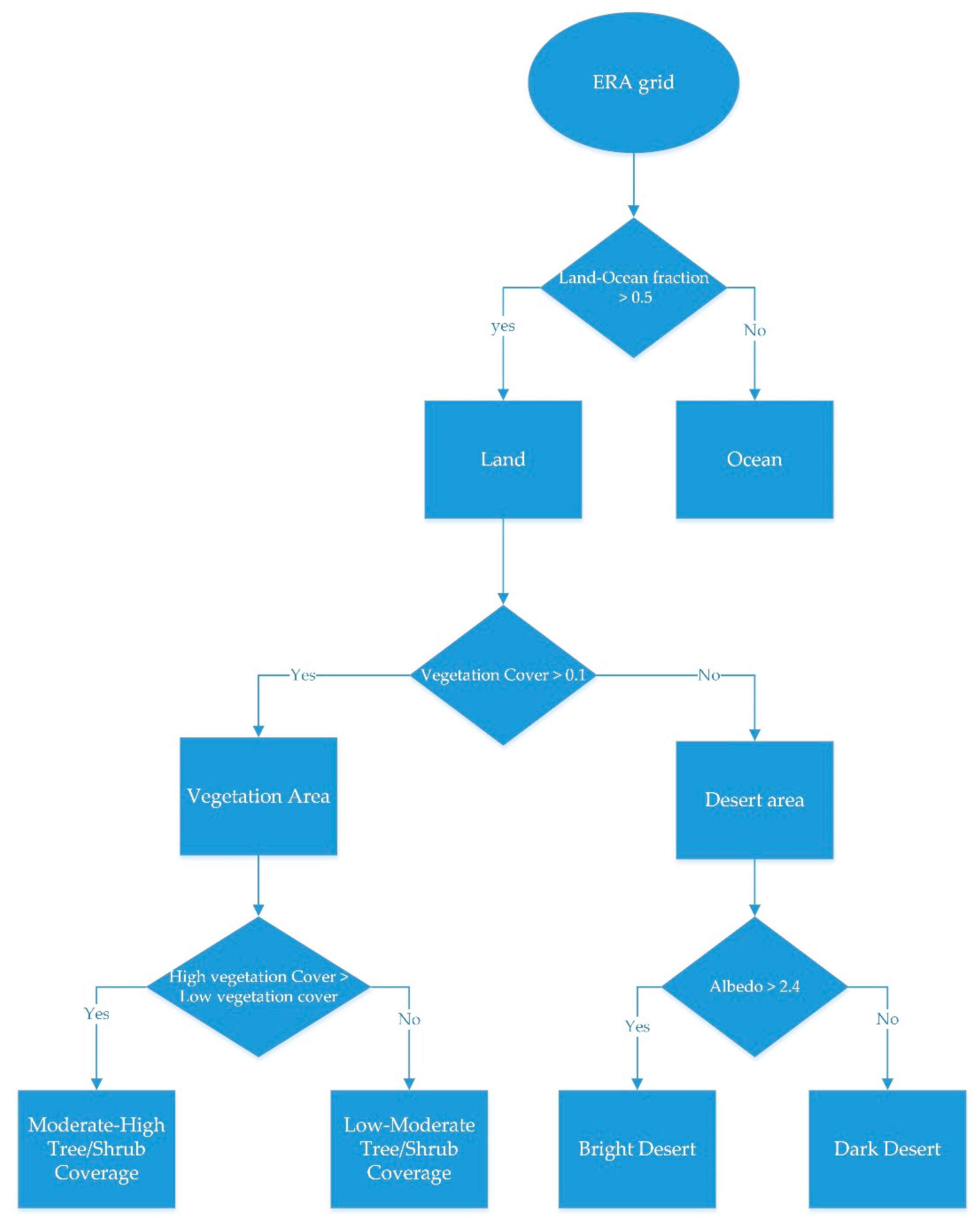
ADMs are derived from the current satellite observation systems for radiative flux studies, e.g., ERBE and CERES. CERES supplies the newest ADMs with better accuracy than ERBE ADMs. There are three types of CERES ADMs, i.e., CERES/TRMM Single Scanner Footprint (SSF) Edition2B ADMs, CERES/Tera SSF Edition2B ADMs, and CERES Terra/Aqua Edition4 ADMs. The major differences among them are the sensor platform, scanning type of the CERES instruments, the algorithm and sensors used to identify the scene type, and even the category of the scene types. In this paper, we used CERES/TRMM SSF Edition2B ADMs (renamed CERES/TRMM ADMs in this paper), due to their accessibility.
The key point when simulating the regional radiance is to identify the scene type of CERES/TRMM ADM for each grid on Earth. There are three category of scene types of CERES/TREMM ADMs: shortwave ADMs, longwave daytime ADMs, and longwave nighttime ADMs. Shortwave ADMs have different parameters to identify the scene types from those of longwave ADMs, as shown in Table 2, because, at longwave, the scattering of the atmosphere and surface is assumed to be independent of the relative azimuth angle, and their emittance contributes more than reflectance. The longwave ADMs have the same parameters but with different classifications between daytime and nighttime. The parameters used to identify the scene types by CERES/TRMM ADMs were derived from the coincident measurements from Visible Infrared Scanner (VIRS) onboard TRMM, atmospheric fields from ECWMF reanalysis, and surface parameters from the International Geosphere Biosphere Program (IGBP) global land-cover types, listed in Table 2 [21].
These chosen parameters in Table 2 have significant influences on the anisotropic characteristics of TOA, and the classification of these parameters follows two statistic principles: (1) the variance of anisotropic factors within each class is smaller than between classes; (2) there are sufficient samples to build up the ADM for each scene type. For shortwave, the land surface type and cloud category determine the albedo of Earth, and their classification is based on the physical definition of each surface or cloud type (see Section 2.4.1 and Section 2.4.2). For the remaining parameters, wind speed over ocean determines surface albedo, optical depth determines the attenuation of shortwave radiative flux, and cloud fraction determines the influence level of cloud. These three parameters are stratified into several intervals to guarantee that there are enough radiance measurements to build up ADMs by CERES/TRMM. The number of intervals and the interval size for the same parameter may vary for different surface types [21]. For longwave, the land surface type and cloud category determine the emissivity of the Earth surface, and they are also classified according to the physical definitions. For the remaining parameters, the vertical temperature change and cloud effective emissivity together indicate the longwave radiative flux from the cloud, the cloud fraction reflects the contribution level of the cloud to the total longwave radiative flux, and precipitable water indicates the absorption of longwave radiation in atmosphere. These four parameters are stratified into the same percentile intervals, according to the frequency distribution of radiance measurements [21]. Thus, the classification of most parameters for both shortwave and longwave in Table 2 is identified through a statistical approach. The global error of CERES/TRMM ADMs is 10 W/m2 at shortwave and 3.5 W/m2 at longwave.
Among the parameters in Table 2, cloud fraction, precipitable water, and wind speed were directly derived from corresponding ERA5 data, which have different names but the same or equivalent definition. Thus, we introduce how to derive the remaining parameters from ERA5 data in the later subsections.

2.4.1. Surface Type

The surface types used by CERES/TRMM ADMs in Table 2 were identified from IGBP land-cover types. The land-cover types with similar anisotropic characteristics are aggregated into the same surface types [21]. For example, all forest land covers, mixed forest, closed shrubland, and woody savannas are classified into moderate–high tree/shrub coverage; savannas, crops, and grassland are classified into low–moderate tree/shrub coverage; open shrubland is classified into dark desert. The IGBP land-cover data used by CERES/TRMM ADMs have a spatial resolution of 10′, while the spatial resolution of the ERA5 grid used in this paper is 1°. This would produce large uncertainty when directly aggregating surface types from IGBP land-cover data. Alternatively, in this case, land–ocean mask, high vegetation cover, and low vegetation cover of ERA5 data were used to identify the surface types for shortwave and longwave, following the principle of surface type determination used by CERES/TRMM ADMs, as shown in Figure 2. Land–ocean mask data supply the fraction of land. For coastal regions, grids with land fraction >0.5 are assigned as land and the rest are assigned as ocean, according to the identification of mixed scene types by CERES/TRMM ADMs [21]. The desert area identified by CERES/TRMM ADMs is the combination of desert and its adjacent open shrubland within a distance less than 10′ [21]. This method could not be applied to the ERA5 grid, due to the coarse spatial resolution. Thus, we followed the identification of the desert area by ERA5 [27], i.e., vegetation cover < 0.1. For shortwave CERES/TRMM ADMs, the dark desert surface is the open shrub land or desert land with shortwave reflectance less than ~22% [21]. Since we did not have reflectance data, ERA5 albedo was applied in this case. According to the retrieved shortwave broadband albedo of semi-desert [28], when the shortwave albedo was larger than 0.24, we classified the desert grid as bright desert; otherwise, it was classified as dark desert. The identification of two vegetation surface types by shortwave CERES/TRMM ADMs emphasized the occurrence of high vegetation. Thus, when the fractional area of high vegetation cover was larger than low vegetation cover, we classified the grid as moderate–high tree/shrub coverage; otherwise, it was classified as low–moderate tree/shrub coverage. For the surface type of longwave in Table 2, vegetation area in Figure 2 was classified as land surface types, and we did not separate dark and bright desert.

2.4.2. Cloud Category

For shortwave CERES/TRMM ADMs, cloud category reflects the different albedo of clouds; ice cloud has higher albedo than liquid cloud. Identification of the cloud category is based on the effective phase index [21], which is defined as the summation of the phase index of liquid and ice clouds weighted by the corresponding fractional area in each grid. The phase index and cloud fraction were derived from VIRS observations. When the fractional area of ice clouds was larger than liquid clouds, the grid was assigned as ice cloud; otherwise, it was assigned as liquid clouds. Since we did not have VIRS measurements on the Moon surface, total column cloud ice water and total column cloud liquid water data in ERA5 were used in this case. We assigned the grid with total column cloud ice water larger than total column cloud liquid water as that covered by ice cloud and vice versa. For longwave CERES/TRMM ADMs, cloud category was directly derived from the cloud fraction, as shown in Table 2.

2.4.3. Cloud Optical Depth

The cloud optical depth reflects the scattering and absorption of aerosol and cloud, which reduces the anisotropic factor in shortwave. For CERES/TRMM ADMs, the cloud optical depth was retrieved directly from the VIRS measurements. ERA5 supplies the TOA incident solar radiation and the total sky direct solar radiation at the surface, the latter of which accounts for the direct solar radiation arriving at the Earth surface and excludes the diffuse solar radiation from the atmosphere and cloud. According to the definition of optical depth ( τ ), we can calculate the cloud optical depth as follows:
τ = ln ( F i F s ) ,
where F i is the radiation received by the top cloud layer, and F s is the radiation transmitted to the whole atmosphere layer and cloud layer and reaching surface. The radiation in Equation (10) is perpendicular to the top and bottom boundary of cloud, such that the influence of viewing angle could be eliminated. The TOA incident solar radiation can be a good estimation of F i , and the total sky direct solar radiation at the surface of ERA5 can be used to estimate F s . Aerosol and atmospheric components, e.g., O2, O3, CO2, and water vapor, can influence our estimation. Cloud, however, is the largest scattering and absorption source of radiance in the path from the top to bottom layers of cloud. Thus, our estimations are acceptable when there is cloud cover.

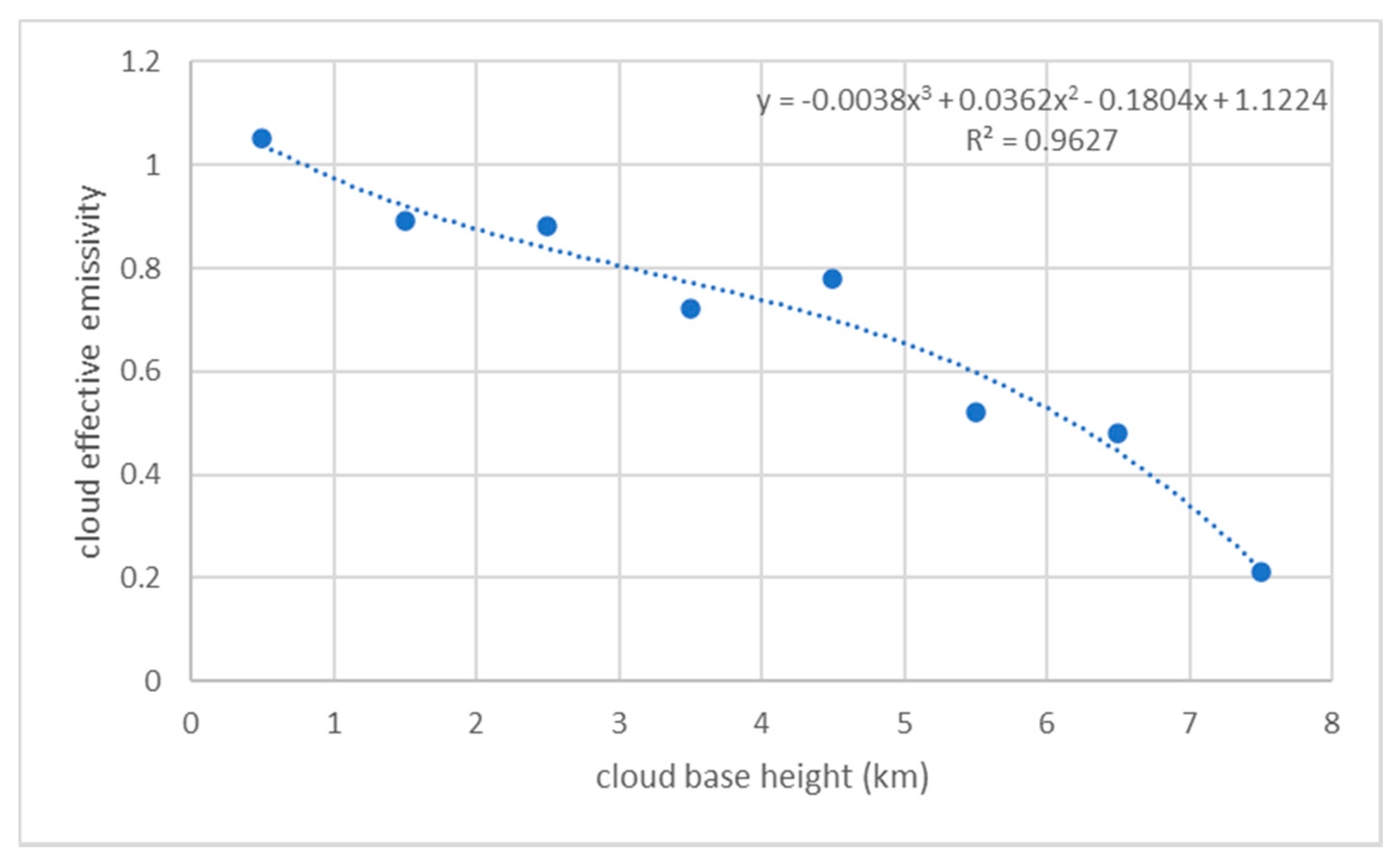
2.4.4. Vertical Temperature Change and Cloud Effective Emissivity

For longwave CERES/TRMM ADMs, vertical temperature change and cloud effective emissivity in Table 2 were used to identify the scene type of TOA [21]. Under cloudy conditions, these two parameters depict the longwave radiative flux from the cloud; a vertical temperature change indicates the cloud height and, thus, the temperature of cloud, whereas cloud effective emissivity at 11 μm indicates the mean emissivity of the cloud at longwave. Under clear sky, the vertical temperature change indicates the lapse rate, which reflects the status of boundary layer [21]. These two parameters are both derived from the VIRS measurements with auxiliary atmospheric data from ECWMF reanalysis. It is difficult to derive VIRS measurements from ERA5. In this paper, we tried to estimate these two parameters purely on the basis of available ERA5 data.
Under clear sky, the vertical temperature change is defined as the temperature difference between surface and air at a pressure level 300 hpa below surface pressure by CERES/TRMM ADMs; under cloudy conditions, this is the temperature difference between the surface and top cloud. Air temperature can be derived from ERA5 multilayer data, while the temperature of the top cloud is difficult to estimate with ERA5 data. Alternatively, ERA5 directly supplies the base height of the cloud; thus, we assumed that the reference level of the cloud layer was at its base height, instead of the top cloud height. In this case, the vertical temperature change ( Δ T ) can be estimated as follows:
Δ T = T s T c ,
where T s is the skin temperature of the surface, and T c is the air temperature at 700 hpa under clear sky and the air temperature at pressure level of the cloud base height for cloudy conditions.
Cloud effective emissivity is defined as the ratio of the difference between observed and clear-sky VIRS 11 μm radiance to the difference between cloud emission and clear-sky radiance by CERES/TRMM ADMs [21]. The cloud effective emissivity cannot be directly derived from ERA5 data, since no such measurements are available. The effective emissivity of the cloud bottom layer is related to the cloud base height, as shown in Figure 3, and it has a good linear relationship with the effective emissivity of the cloud top layer [29]. Thus, we estimated the cloud effective emissivity ( ϵ e f f ) from the cloud base height (h in km) as follows:
ϵ e f f = 0.0038 h 3 + 0.0362 h 2 0.1804 h + 1.1224 .
The cloud emissivity in Figure 3 is the mean value of observed emissivity within each 1 km interval of cloud base height starting from 0 km; thus, a more robust model to derive cloud emissivity from cloud base height would be a type of Gaussian process. Since we did not have the deviation data of cloud emissivity for each interval of cloud base height, Equation (12) was used as an approximation of real cloud effective emissivity. Figure 4 shows the cloud fraction, TOA longwave radiative flux and estimated cloud effective emissivity at UTC 3:00 p.m. on 11 February 2017. It is clear that the emissivity at the high cloud fraction is high, which follows the understanding of cloud emissivity. The cloud effective emissivity in Figure 4c is in good agreement with the longwave radiative flux in Figure 4b. Thus, the method of Equation (12) follows the pattern of longwave radiative flux from clouds in general.
The accuracy of our estimation of these two parameters with ERA5 needs further studies. The classification of these two parameters used to identify the scene types of CERES/TRMM ADMS, however, tolerates possible errors in our estimation. When the remaining parameters are fixed, vertical temperature change can be stratified into four classes with the same percentile interval according to the frequency distribution of radiance measurements used to build up the ADM. Cloud effective emissivity is also stratified in the same way. When the remaining parameters are changed, the stratification interval of the vertical temperature change or cloud effective emissivity also varies. For example, when a cloud is over ocean, the cloud effective emissivity interval for the first 25% of radiance observations ranges from 0 to an upper boundary. For high clouds (with large vertical temperature change values), the upper boundary of cloud effective emissivity is between 0.28 to 0.44, increasing with the cloud fraction; for low clouds (with small vertical temperature change values), the upper boundary ranges from 0.39 to 0.60 [21]. Thus, the stratification intervals of cloud effective emissivity are related to the other parameters, e.g., cloud height and cloud fraction, and they together reflect the status of the cloud. Our estimations of vertical temperature change and cloud effective emissivity are directly derived from the status of the cloud, e.g., the cloud base height, using statistical models. This guarantees that our estimation is reasonable and falls into a correct ADM scene type.

3. Results

We first calculated the viewing geometry of the Earth–Sun–Moon for each ERA5 grid on the Earth surface at each hour of 2017 and determined the grids in the view of an observer on the Moon surface. The parameters used to identify the scene type of CERES/TRMM ADMs were derived from ERA5 data at the same time. The anisotropic factor of each grid was determined from the identified ADM according to the viewing geometry. The regional radiance of each ERA5 grid in the Moon-based view was calculated using Equation (5). The global mean radiance, global mean radiative flux, and global mean ADM of the whole Earth in the Moon-based view were calculated according to the method developed in Section 2.3. The simulated global mean radiance is demonstrated in Section 3.1 and Section 3.2, together with the global mean TOA outward radiative flux. The global mean ADM of the whole Earth is illustrated and analyzed in Section 3.3. FFT was used here to illustrate the spectral information of time series of the simulated radiative flux and radiance.

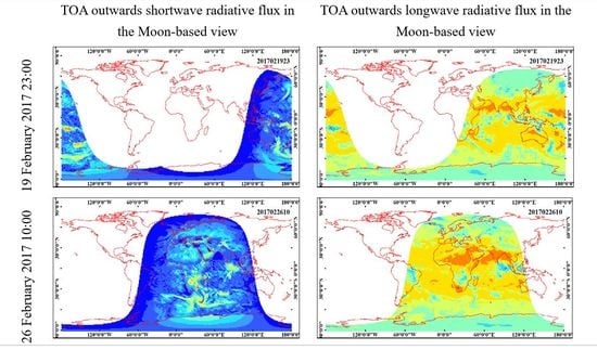
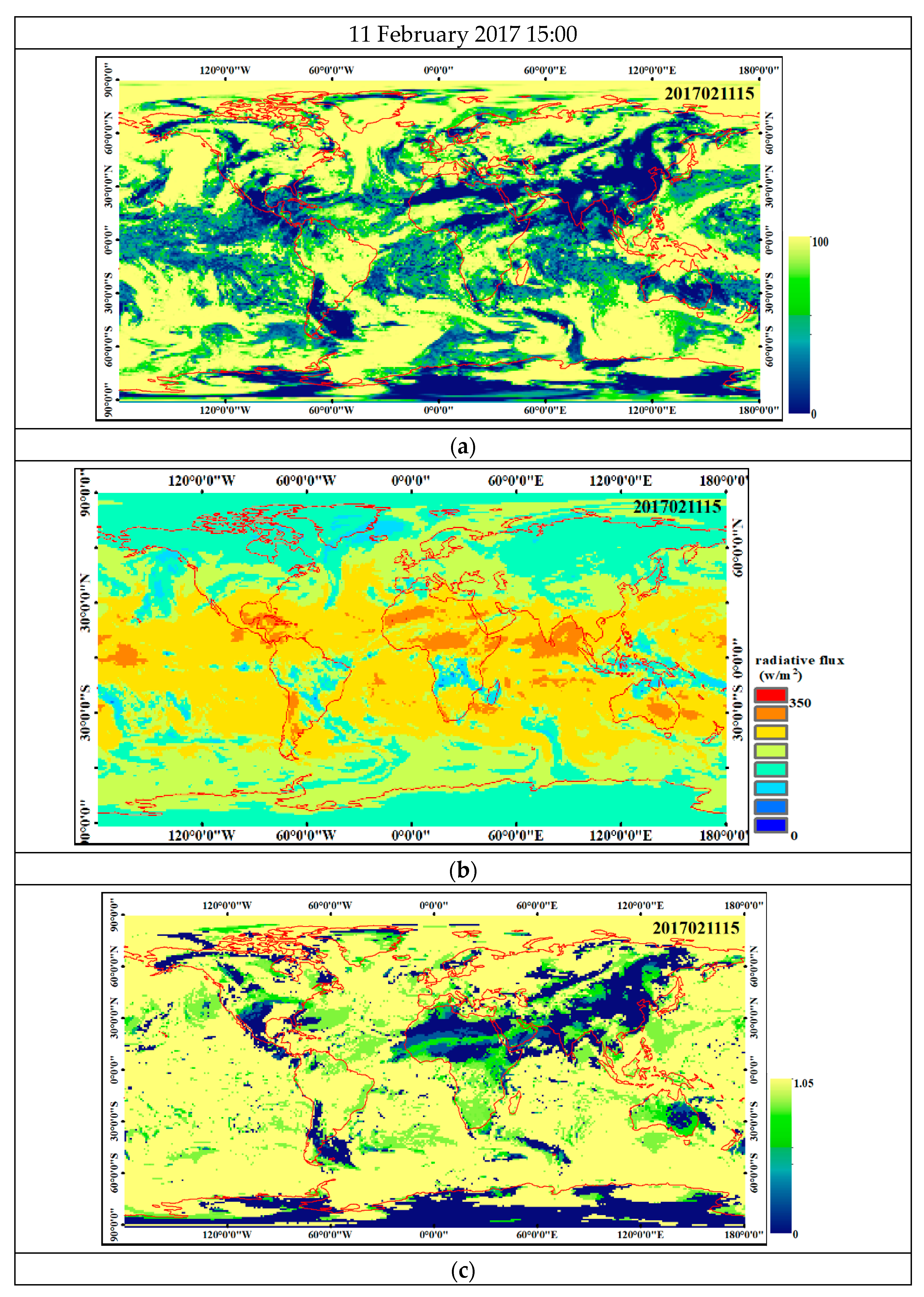
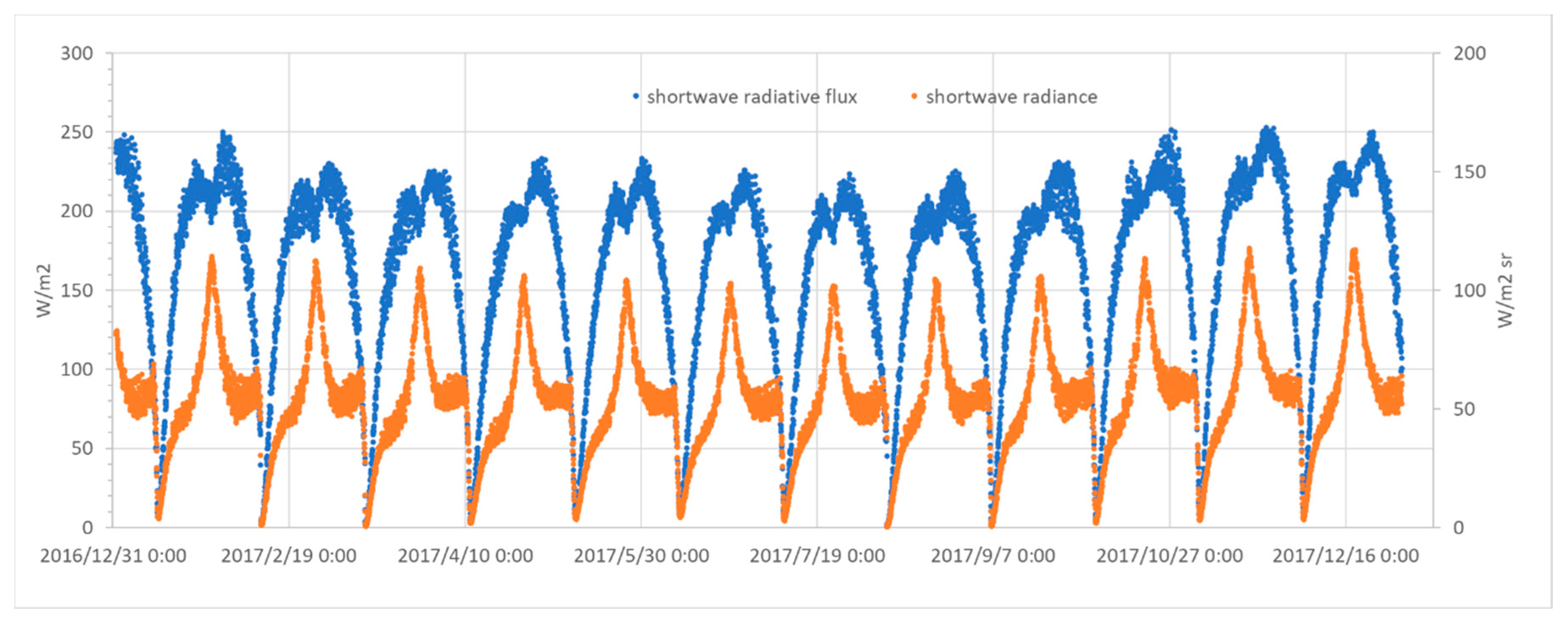
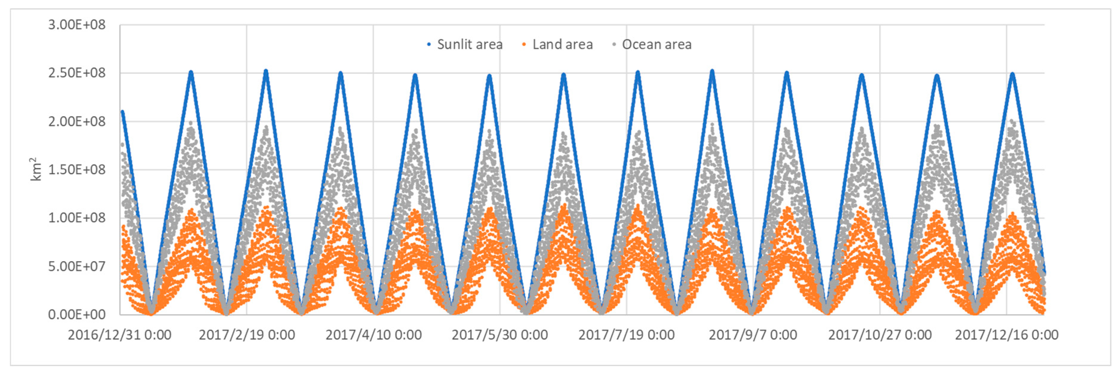
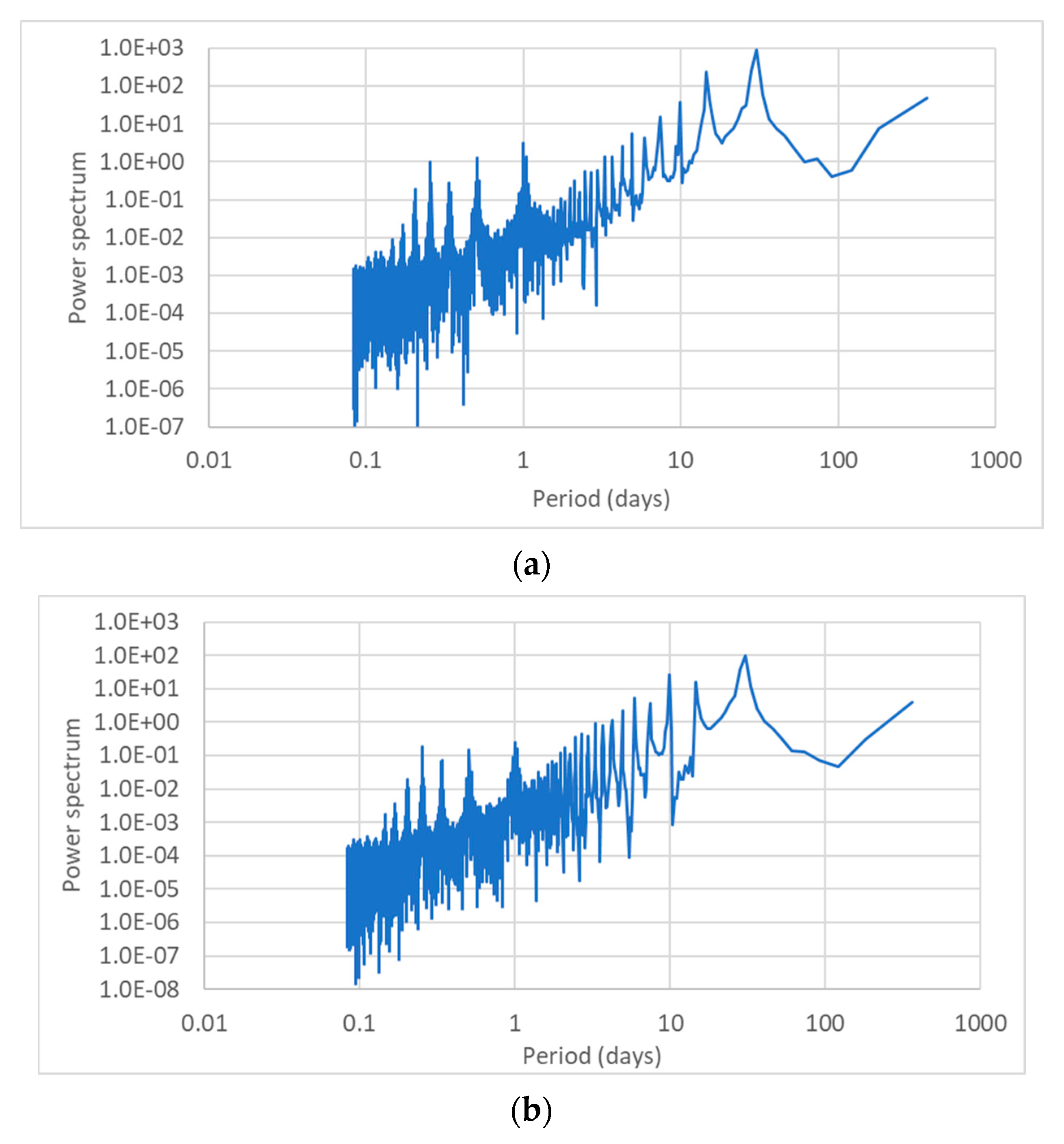
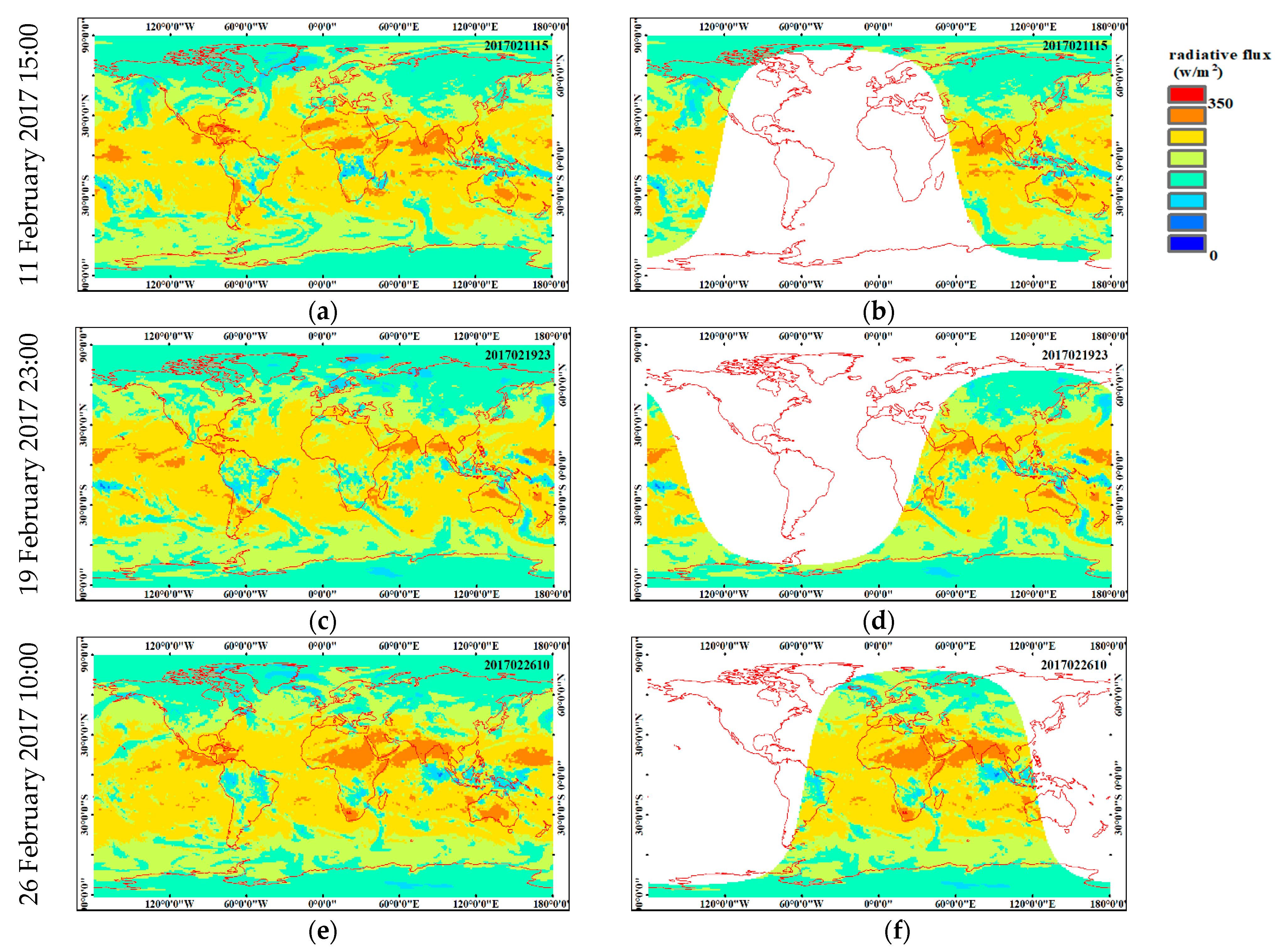
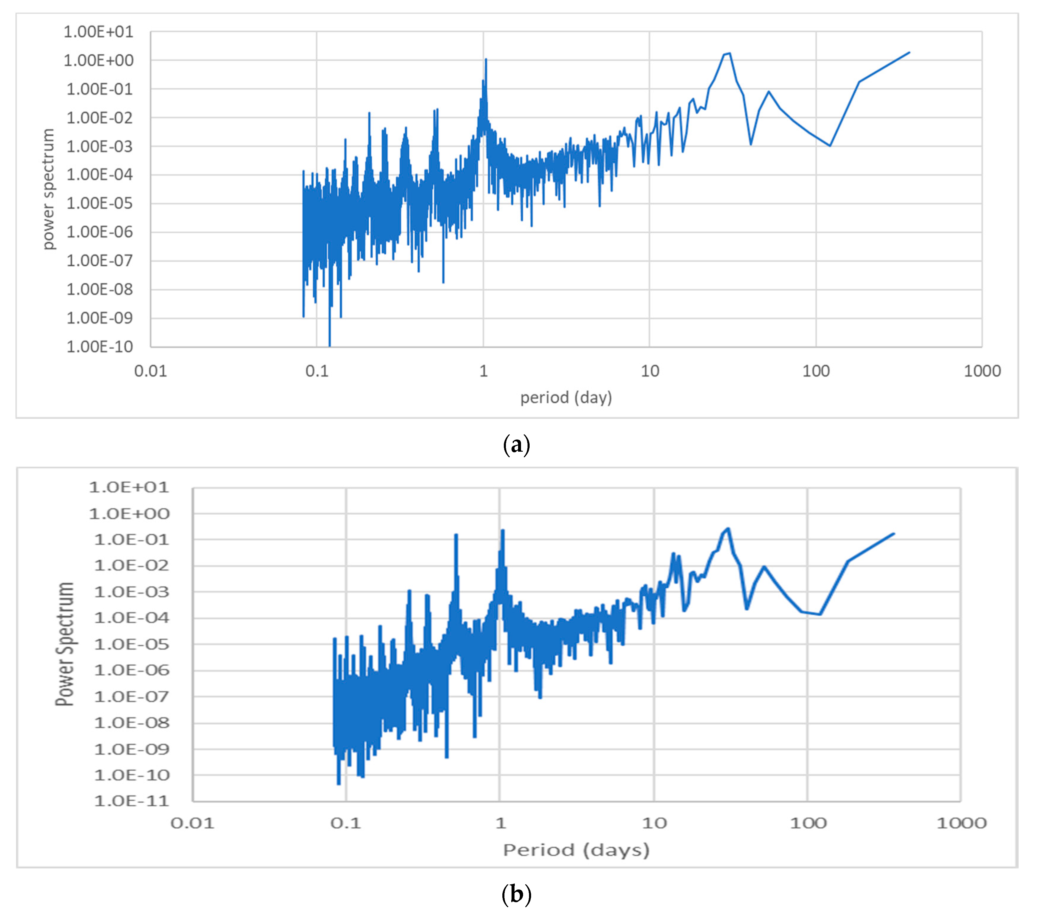
3.1. Global Mean Outward Shortwave Radiative Flux and Its Radiance of Earth in the Moon-Based View

The sunlit area, illustrated as the positive shortwave outward radiative flux, moves from east to west on the Earth surface within 1 day due to Earth rotation, as shown in Figure 5a,c,e. The Earth obliquity leads to movement of the sunlit area between the northern and southern hemispheres of the Earth. Only part of the Earth surface visible to the Moon is illuminated by the Sun, while the remainder is on the shadow side of the Earth (nighttime), as shown in Figure 1b. When the Moon revolves around the Earth, the sunlit area moves from the eastern edge of the Earth disc in the Moon-based view to the center, as shown in Figure 5d,f and then it moves from the center to the western edge. Due to the inclination angle of Moon–Earth orbits, two stripes on the Earth surface in the Moon-based view can be illuminated by the Sun, as shown in Figure 5b. This phenomenon can be observed in our daily life; sometimes, just before sunset (the western stripe in Figure 5b) or after sunrise (the eastern stripe in Figure 5b), the Moon can be observed in the sky together with Sun. The combination of Earth rotation and Moon revolution complicates the sunlit Earth surface in the Moon-based view. When we take the sunlit area of the Earth surface in the Moon-based view as one point, it is difficult to define the viewing zenith angle for this point, because the curvature of the Earth surface leads to variations in the viewing zenith angle for each grid on the Earth surface. The sunlit areas at the center of the Earth disc in the Moon-based view have small viewing zenith angles, while those at the edge have large viewing zenith angles. Since the sunlit area of the Earth surface in the Moon-based view increases from the edge to the center and then decreases from the center to the edge when the Moon revolves around Earth, the size of the sunlit area of the Earth surface in the Moon-based view was used to indicates the changes in the overall viewing zenith angle, in this case.
The global mean outward shortwave radiative (OSR) flux emitted from the whole sunlit area of the Earth surface in the Moon-based view (simulations were calculated using Equation (9), and the results are shown in Figure 6) is different from the total Earth TOA OSR flux, and it varied from 0 to ~250 W/m2 in 2017. The global mean shortwave radiance was simulated from regional radiance using Equation (7), and it varied from 0 to ~120 W/m2sr. The peak values of the global mean shortwave radiance occur when the sunlit area of the Earth surface in the Moon-based view reaches its maximum, as shown in Figure 7; at the same time, the global mean OSR fluxes are very close to the mean shortwave radiative flux of Earth derived from CERES Synoptic flux product (SYN1deg) data according to the Earth–Sun–DSCOVR geometry [12], but reside in the trough of the whole time series. The peak values of global mean OSR fluxes occur when the sunlit area is smaller than its maximum, because small OSR fluxes at the edge of the sunlit Earth surface is not in the Moon-based view. For example, Figure 5c shows the full picture of the outward shortwave radiative flux, where the area in America have low radiative flux (close to the local evening). Figure 5d illustrates the sunlit Earth surface in the Moon-based view, where the sunlit area in America was not visible to the Moon view. In such a case, the global mean radiative flux of the sunlit Earth surface in the Moon-based view is higher than that of the sunlit area of the whole Earth.
We can observe clear monthly periodic changes in the time series of the global mean OSR flux and the global mean shortwave radiance. The FFT algorithm was used to calculate and analyze the power spectrum of these two time series, as introduced in [20]. The largest peak in the power spectrum of the time series of the global mean OSR flux in Figure 8a was the frequency component with a period of 30.42 days, followed by a secondary component with a period of 14.04 days, a third one with a period of 365.0 days, and a fourth one with a period of 9.61 days. The power spectrum of the time series of the global mean shortwave radiance was similar to that of the global mean OSR flux, although their time series showed large differences. The frequency components with periods of 30.42 days, 9.86 days, 365.0 days, and 14.02 days in the power spectrum of the shortwave radiance (Figure 8b) had peak values, but with a different order from those in the power spectrum of the global mean OSR flux. The frequency components with peak powers in the power spectrum of these two time series indicated the factors influencing the radiative flux of the Earth surface in the Moon-based view, as discussed in Section 4.

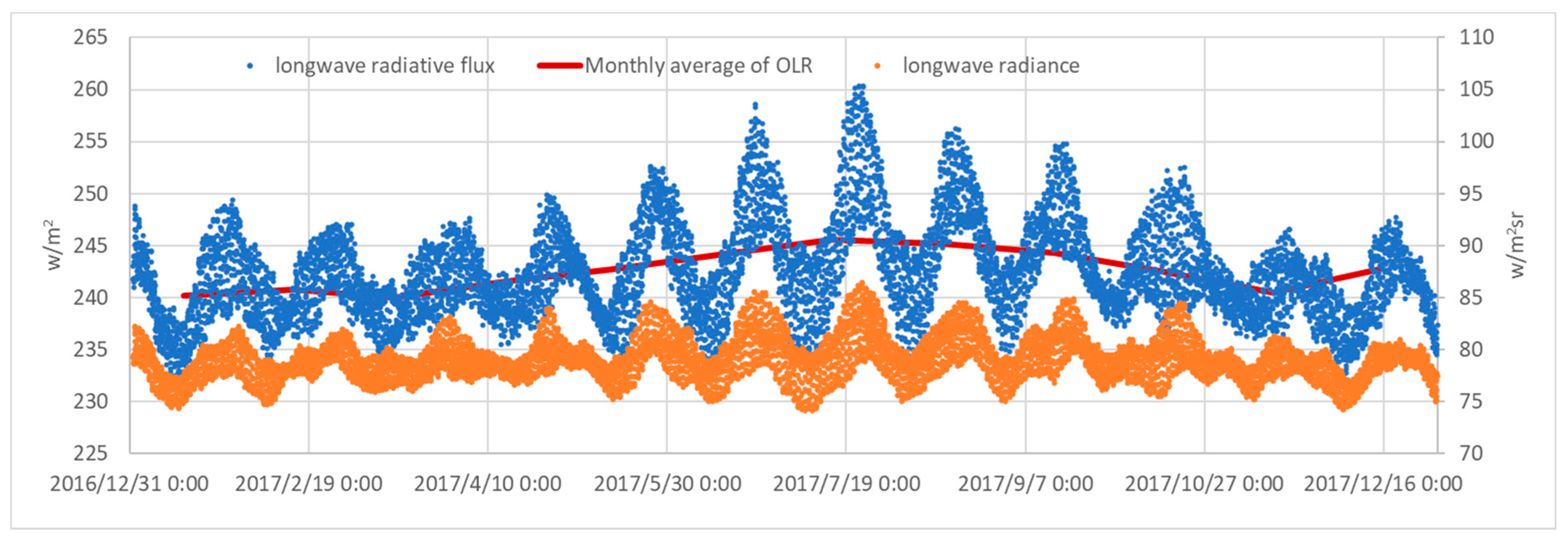
3.2. Global Mean Outward Longwave Radiative Flux and Its Radiance of Earth in the Moon-Based View

Outward longwave radiation (OLR) emitted from almost half the Earth surface was in the Moon-based view, as shown in Figure 9. The rotation of the Earth and the lunar orbital inclination lead to different areas of the Earth surface being in the Moon-based view at different observation times (see Figure 9). When the Moon revolves from the conjunction position to the opposite position of its orbit, the sunlit area of the Earth surface in the Moon-based view changes from its maximum to the minimum (see Figure 7), while the shadow Earth area in the view changes synchronously but in a reverse way. The global mean OLR flux of the Earth in the Moon-based view calculated with Equation (9) varied from 230 to ~260 W/m2, and the global mean longwave radiance calculated with Equation (7) varied from 70 to 80 W/m2sr, as shown in Figure 10. There is a clear monthly cycle in the time series of the global mean OLR flux and the global mean longwave radiance, due to the periodic sunlit/shadow area changes in the Earth surface visible to the Moon-based view. In Figure 10, the peak global mean OLR fluxes occurred when the sunlit area in the Moon-based view reached its maximum; on the other hand, extremely low OLR fluxes occurred when the shadow Earth surface in the Moon-based view reached its maximum. The peak values of the global mean OLR fluxes (Figure 10) consisted of the upper envelope of the time series and showed a clear seasonal change in 2017. They increased from February, reached the maximum in July, and then decreased, reaching the minimum in November, followed by a slight increase, reaching a second peak in January. This variation in the peak values of global mean OLR fluxes is similar to that of OLR fluxes of the sunlit side of Earth derived from CERES SYN1deg data [12], according to the Earth–Sun–DSCOVR geometry. The extremely low values consisted of the lower envelope of the time series of global mean OLR fluxes and had the opposite tendency to the upper envelope in Figure 10. This reverse tendency between upper and lower envelopes of the time series of OLR led to the amplitude of the variation in each month cycle increasing gradually from February to July and decreasing after August, as shown in Figure 10. The global mean longwave radiance of Earth surface in the Moon-based view varied in the same pattern with the global mean OLR fluxes. The induced global ADM seemed to have little impact on the variation of radiance. The difference in the spectral features between the power spectrum of the time series of the global mean OLR flux and the global mean longwave radiation was small, as shown in Figure 11. They both had the same frequency components with periods of 365 days, 30.4 days, and 1.03 days having the largest peak values, as shown in Figure 11. The possible causes of the variation characteristics of the global mean OLR flux and its radiance are discussed in Section 4.

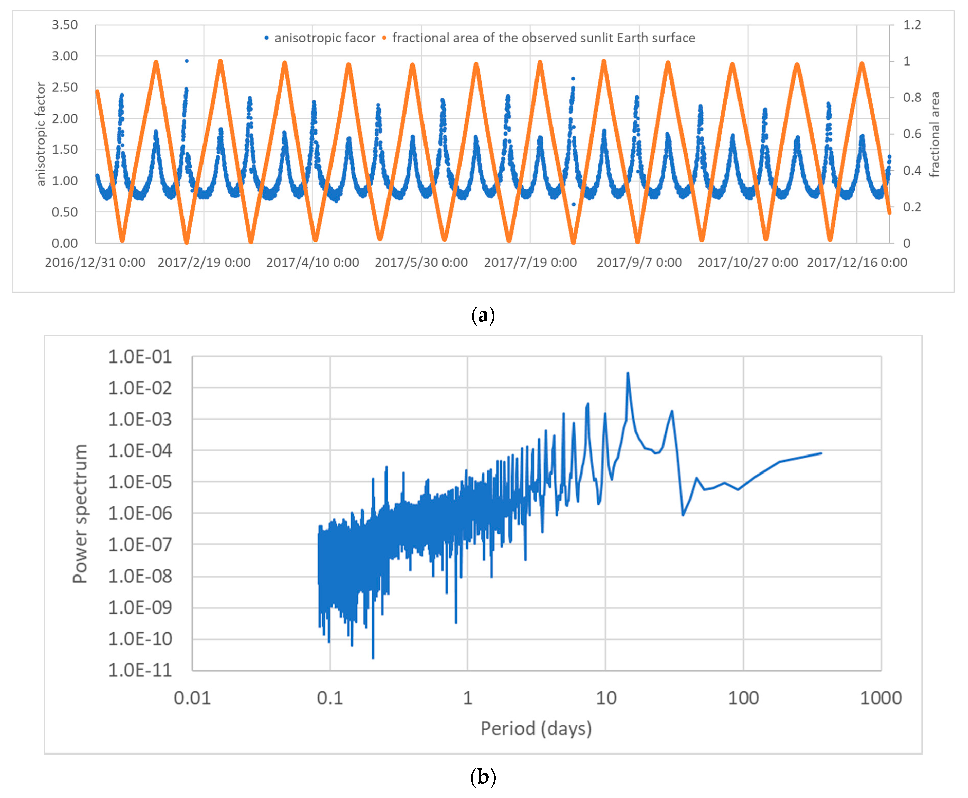
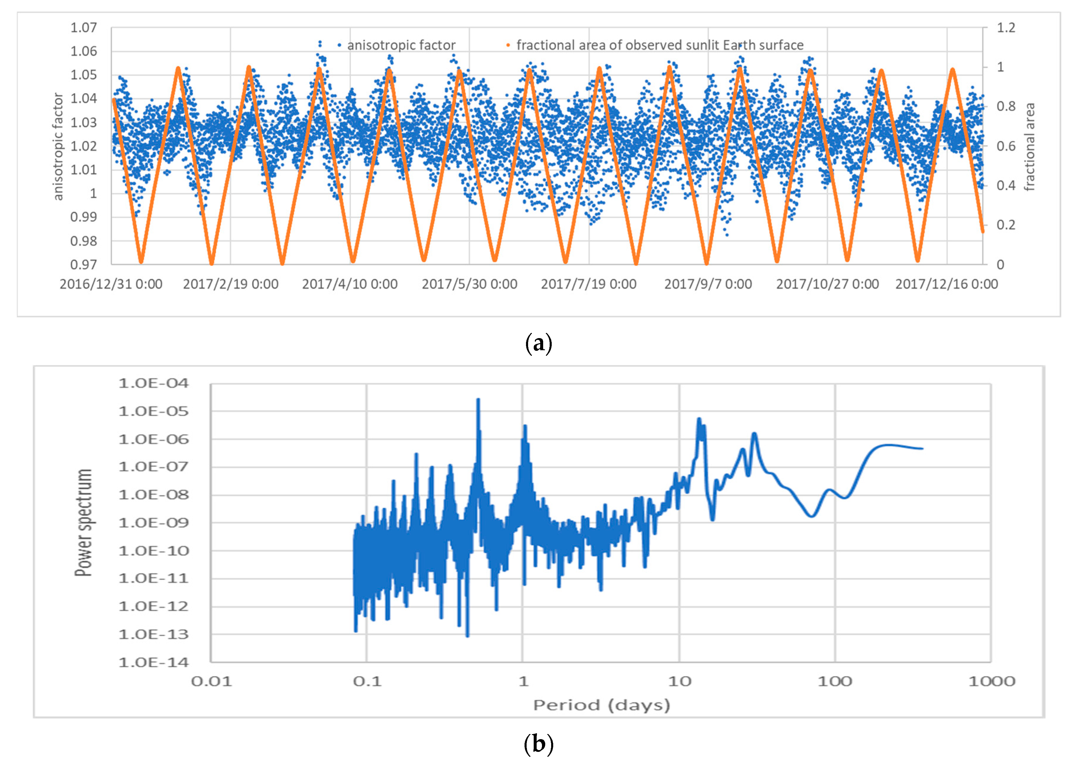
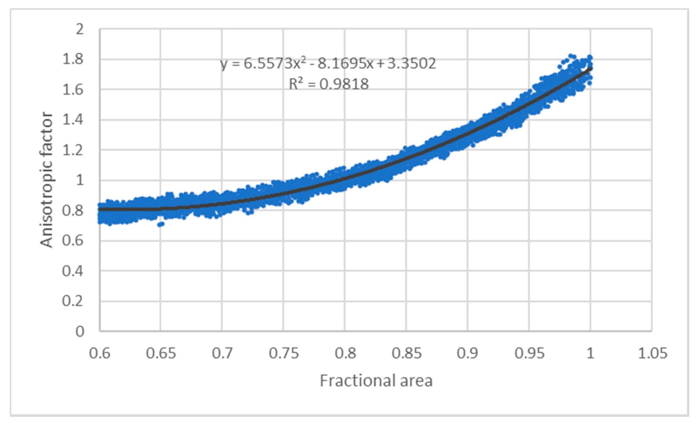
3.3. Anisotropic Factor of the Global ADM

The global ADM is a function of observation time in Equation (6), and it was derived using global mean radiative flux calculated with Equation (9) and global mean radiance calculated with Equation (7). The anisotropic factor of the global shortwave ADM is shown in Figure 12, together with the power spectrum of its time series. The global shortwave anisotropic factor varied between 0.5 and 2.5 and had a clear periodical cycle, as shown in Figure 12a. In the power spectrum of the time series of the global mean anisotropic factor of shortwave (Figure 12b), the frequency component with a period of 14.6 days had the largest peak value. The daily variation was small in the global anisotropic factor of shortwave. The fractional area of the sunlit Earth surface observed in the Moon-based view was calculated as the ratio of the observed sunlit area to the maximum sunlit Earth area observed in the total 1 year period. The global anisotropic factor reached a peak when the peak fractional area of the observed sunlit Earth surface occurred. When the fractional area of the observed sunlit Earth surface was close to 0.4, the global anisotropic factor reached a trough with a value around 0.7. When the fractional area of the observed sunlit Earth surface was less than 0.4, the global anisotropic factor quickly increased to around 2.5.
When the fractional area of the sunlit Earth surface in the Moon-based view reached its maximum, the center of the Earth surface visible to the Moon-based view was illuminated nearly perpendicularly by Sun; thus, the viewing zenith angle and the solar zenith angle of the center area were both close to 0°. In this condition, the regional ADMs of both land and ocean cover would reach a peak, regardless of the cloudy conditions, according to the CERES/TRMM ADMs [21].
The global anisotropic factor of longwave was calculated in a similar way to that of shortwave, and it varied between 0.99 and 1.07, as shown in Figure 13a. For the sunlit Earth area in the Moon-based view, daytime CERES/TRMM ADMs were used to calculate the radiance; for shadow Earth area, nighttime ADMs were used. Due to the two different classes of ADMs used in our simulation, in a monthly cycle, the global longwave anisotropic factor had two peak values; one occurred when the fractional area of the observed sunlit area reached its minimum, while the other occurred when the fractional area of sunlit Earth reached its peak, as shown in Figure 13a. In the power spectrum of the time series of the global anisotropic factor of longwave, the largest three peak values occurred in the frequency components with periods of 0.52 days, 13.52 days, and 1.05 days.

4. Discussion

4.1. Impact of Earth Climate on the Radiance of the Earth Surface in the Moon-Based View

When we measure the radiance of Earth outward radiative flux in the Moon-based view, as shown in Figure 1, the whole Earth is observed as one pixel object, whereby the Earth is a thermodynamic system whose external forcing (mainly from solar radiation) and outward radiation are generally in balance. ECS allocates the solar radiation into the different components, and it shapes the shortwave and longwave radiation of the whole Earth outward to space [1,2]. With climate reanalysis, i.e., ERA5 in this paper, global mean OSR fluxes and global mean OLR fluxes of the Earth surface in the Moon-based view were derived, and their radiance was calculated using CERES/TRMM ADMs. Clear periodical signals were induced in the time series of derived global mean radiative fluxes and their radiance, as shown in Section 3.1 and Section 3.2. According to [20], if one time series is a function of some parameters, the power spectrum of the time series includes the spectral features of its contained parameters. Thus, some of these signals are probably related to the Earth climate, as discussed in this section; the remainder are probably related to the Earth’s rotation and the Moon’s orbit, as analyzed in Section 4.2.
In addition to the clear monthly cycle, which was probably due to the Moon’s orbit, in the time series of the global mean OSR flux (Figure 6), the annual cycle was also obvious, and it had the third largest peak power in its power spectrum (Figure 8a). From the changes in the upper envelope of the time series of the global mean OSR flux in 2017, we could find that OSR flux decreased from February to July and then increased again. After taking the anisotropic characteristics of TOA into account, this annual cycle persisted in the time series of the global mean shortwave radiance (Figure 6) and could be observed clearly in its power spectrum (Figure 8b). There might be two sources of this annual cycle: (1) instant incident solar radiation changes with Earth–Sun distance varying between perihelion and aphelion positions [12]; (2) seasonal changes in the Earth albedo. The second reason may contribute more than the first, since the solar radiation accumulated over a period of time is constant according to Kepler’s second law. The daily variation in OSR flux and its radiance is mainly due to the Earth’s rotation, which induces changes in the cloud fraction and its physical properties. The global mean OSR flux and its radiance do not have large daily variations, as shown in Figure 6, and the power of the daily frequency component is much smaller than that of components representing the monthly and annual cycles in the power spectrum, as shown in Figure 8. Our simulation indicated that the cloud influence on outward shortwave radiation is relatively small in the Moon-based view, which is probably due to the rapid reduction in sunlit Earth surface, as shown in Figure 7.
The global mean OLR flux of the Earth surface in the Moon-based view (Figure 10) had obvious daily variations, with clear monthly and annual cycles. Similar features could also be observed in the time series of global mean longwave radiance, which could be determined from the spectral features in the power spectrum of the OLR flux and its radiance. To remove the daily variations, the monthly average of the global mean OLR flux was calculated in Figure 10, and it showed a tendency opposite to the global mean OSR flux, which is probably due to the energy balance of the Earth and indicates that the changes in Earth albedo may be the major source of the annual cycle in both OLR and OSR fluxes. The daily variations in the global mean OSR flux and its radiance were larger than those in the OSR flux and its radiance, despite being related to the same factors, i.e., the Earth’s rotation and the changes in cloud properties. The major reason for this discrepancy is that the area of the Earth surface in the Moon-based view that contributes to the outward radiation is different. For longwave, both the shadow side and the sunlit side of the Earth surface in the view contribute to the outward radiation (L1 and L2 regions in Figure 1b); for shortwave, only the sunlit area of the Earth surface in the view is considered. Rapid changes in the sunlit Earth surface in the view suppress the daily variations in the shortwave radiative flux. However, periodical changes in the sunlit Earth area in the Moon-based view (in Figure 7) induce the monthly cycle in the global mean OLR flux and its radiance.
The variation characteristics in the time series of the global mean OLR flux indicate the influences of the Earth’s climate, albedo, and obliquity on the Earth energy budget. The OLR flux is closely related to the Earth surface temperature, especially under clear-sky conditions [30,31]. The variations in the global mean OLR flux in Figure 10 directly reflect the changes in global averaged surface temperature of the Earth. In March and September, the maximum insolation is close to the equator, and the northern and southern hemispheres are equally illuminated by solar radiation. Near the equinox days, the temperature gradient along the latitude is close to the symmetric condition [32,33]. Since the maximum insolation is close to the equator, the hotspot of surface temperature is in the tropic zone, where the diurnal variation in surface temperature is small. Thus, in February, March, and October of 2017, the peak OLR fluxes were close to these extreme low values, and the amplitude of monthly cycle was small. When the maximum insolation moves southward or northward, the hotspot of surface temperature moves simultaneously and leads to the asymmetric distribution of surface temperature [32,33]. The sunlit Earth surface simultaneously comprises the surface in winter and summer in both hemispheres, as does the shadow Earth surface. Due to the Earth’s obliquity, in summer, the area of sunlit Earth surface with a relatively high temperature in summer is larger than that with a relatively low temperature in winter, whereas the area of shadow Earth surface with a relatively high temperature is smaller than that with a relatively low temperature. The most evident phenomena are the polar day and polar night. Thus, the spatially averaged surface temperature of sunlit Earth in summer/winter is higher than that in spring/autumn; the spatially averaged surface temperature of shadow Earth in winter/summer is smaller than that in spring/autumn. This probably explains why the peak OLR fluxes increased from March to July and from November to January in 2017, whereas the extremely low OLR fluxes, reflecting the surface temperature of shadow Earth, decreased from April to July and from November to January.
The monthly amplitude in the time series of the global mean OLR fluxes (in Figure 10) reflects the heating rates of Earth, since the sunlit Earth surface in the Moon-based view changes periodically from its minimum to its maximum with the revolution of the Moon, as shown in Figure 7. When the maximum insolation moves southward or northward from the equator, in the sunlit Earth surface, the recession area of snow and ice becomes gradually larger than the increased area of snow and ice, mainly due to the obliquity of the Earth. Although the specific heat capacity of snow and ice is smaller than that of water, the large thermal conductivity of snow and ice leads to the rapid transfer of surface heat to deep layers. In addition, the high albedo of the snow/ice surface leads to less absorption of solar radiation, compared with the water surface. These factors mean that, when ice/snow is melting, more solar radiation is absorbed by the Earth surface and increases the surface temperature [34]. The surface type changing from snow/ice to water probably dominates the monthly amplitude increase when the maximum insolation moves to the southern hemisphere.
When the maximum insolation moves to the northern hemisphere, in addition to the changes in snow/ice coverage, the increases in vegetation coverage and leaf area index (LAI) also contribute to gradually increasing the heating rates from March to July. Compared with dry bare soil or desert, vegetation has low albedo and, thus, absorbs more solar radiation [34,35]. The temperature of the vegetation canopy, however, does not increase as quickly as that of bare soil, mainly due to the evapotranspiration. More solar radiation is transferred into latent heat by vegetation, so as to keep the vegetation surface cool and force the movements of air and water. The kinetic energy enhances the heat transfer from warm regions to cool regions through the atmosphere. The increased water vapor in the atmosphere enhances the hydrological cycle [36]. The latent heat stored in the atmosphere is released to sensible heat via condensation and precipitation. Thus, vegetation changes the heating rate of the Earth, and this influence could be observed from the changes in the monthly amplitude of the time series of the global mean OLR flux from March to July (see Figure 10). The above variations in the global mean OLR flux also persisted in the global mean longwave radiance observed in the Moon-based view. Overall, long-term observations of OLR on the Moon surface would directly reflect the climate change of the whole Earth.

4.2. Implication for Exoplanet Studies from Moon-Based Radiatiance Observations

It is very important for exoplanetary research to identify the rotation period and its orbital information from the observed spectral data [5,37]. In previous studies, the changes in sunlit area were seldom considered. The sunlit exoplanet surface in the view of Earth, however, may be periodically due to the revolution of the exoplanet, similar to the sunlit Earth surface in the Moon-based view. With this change in sunlit surface in the Moon-based view, variations in both shortwave and longwave radiance had a strong monthly cycle, as shown in Figure 6 and Figure 10, with frequency components of 30.42 days, 14.04 days, and 9.61 days having peak values in their power spectrum, as shown in Figure 8b and Figure 11b. These frequency components were directly related to the sunlit Earth surface in Figure 7. Among these three frequency components, the component with 30.42 days had the largest power, related to the revolution period of the Moon. In the power spectrum of longwave radiance (Figure 11b), the daily variation was very significant, probably related to the rotation of the Earth. The rotation of the Earth introduces various surface and atmospheric conditions into the view. In shortwave radiance, the daily variation is weak but observable.
The global ADMs of both shortwave and longwave varied with time for the observed radiance in the Moon-based view, as shown in Figure 12 and Figure 13. The effect of anisotropic characteristics on the spectral analysis of exoplanets needs more consideration, especially when we want to identify the components in the atmosphere and cloud of an exoplanet [38]. Through the simulations, we found that the global anisotropic factor of shortwave is closely related to the area of sunlit Earth surface in the Moon-based view, especially then the fractional area of the sunlit surface is larger than 0.6, as shown in Figure 14. Thus, we introduce a simple method to derive the global mean shortwave anisotropic factor for an exoplanet ( R ¯ ( x ) ) with atmospheric components similar to Earth as follows:
R ¯ ( x ) = 6.56 x 2 8.17 x + 3.35 ,
where x is the fractional area of the sunlit (daytime) exoplanet in the view. With Equation (13), the global mean anisotropic factor of shortwave is related to its sunlit (daytime) surface, instead of the observation time. This would reduce the complexity in building up a high-accuracy geometric model. The uncertainty of the model in Equation (13) is around 0.2. When the viewing geometry is similar to that of NISTAR, i.e., the fractional area of the sunlit surface is close to 1.0 (see Figure 14), the global anisotropic factor of shortwave has uncertainty as large as 0.3. This indicates that the global anisotropic factor of shortwave used by NISTAR is more sensitive to cloud physics, ocean winds, and surface types. Thus, more research is needed if we want to reduce the uncertainty in Equation (13), by taking the surface and cloud conditions into account. Since the sunlit surface in the Moon-based view overlaps that of the DSCOVR view, the anisotropic factor derived from Moon-based observations would help to calibrate that used by NISTAR. Meanwhile, the global anisotropic factor of longwave in the Moon-based view also fluctuates, as shown in Figure 13a. Its range, however, is small, especially when the fractional area of the sunlit surface close to 1.0. A constant global anisotropic factor of longwave could be used by NISTAR to evaluate its error sources.

4.3. Error Analysis for the Simulations

The error in our simulations of regional radiance ( E ( I ^ ) ) can be expressed as follows:
E ( I ^ ) = E ( d a t a ) + E ( A D M ) + E ( S ) ,
where E ( d a t a ) is the error due to the reanalysis, E ( A D M ) is the error due to the ADMs, and E ( S ) is the error due to our methods used in identifying the scene types of ADMs. Since we calculated and analyzed the global radiance in this case, the error E ( I ¯ ) can be calculated as follows:
E ( I ¯ ) = j = 1 N E ( d a t a j ) + j = 1 N E ( A D M j ) + j = 1 N E ( S j ) ,
where E ( d a t a j ) , E ( A D M j ) , and E ( S j ) are the reanalysis error, ADM error, and the error of our method used in identifying the ADM scene type for j-th grid on the Earth surface in the Moon-based view, and N is the total number of grids in the view. The error of global ADM is similar to that in Equation (15).
ERA5 is the newest version of reanalysis developed by ECWMF. The accuracy of longwave and shortwave radiation of ERA5 has been studied at several locations, better than other reanalysis methods [23,39]. At the global scale, however, there is need for more studies and further analysis. In our simulations, OSR of the whole sunlit Earth surface was close to that derived from CERES SYN1deg data, while OLR was larger [12]. The cause of the difference in OLR is unknown. Possible reasons could be related to the aspect of CERES, i.e., the uncertainty in the derivation of broadband longwave radiance from multiband observations and in the derivation of the anisotropic factor under thin clouds, or from an overestimation by ERA5. The global mean error introduced by CERES/TRMM ADMs to the radiation flux was 10 W/m2 at shortwave and 3.5 W/m2 at longwave, for all-sky conditions [40]. The errors in the ADMs and our methods used in identifying the scene types of ADMs were closely related. In the shortwave, most parameters in Table 2 were directly derived from ERA5, while, in the longwave, the vertical temperature difference between surface and cloud and the cloud effective emissivity were estimated from cloud base height, which may have introduced large uncertainty. This uncertainty was mitigated by the stratification method used to identify scene types [21].
It is reasonable to assume that errors in the reanalysis and ADM in Equation (15) had a mean of zero and a certain deviation. Equation (15) integrates errors of the grids in the view, whereby when the number of grids involved is increased, the global error in the reanalysis and ADM would be mitigated [11,12]. This could be proven from the global shortwave ADM at a certain level. When the fractional area of the sunlit Earth surface in the view was larger than 0.6, the variation in the global shortwave anisotropic factor was relatively small, as shown in Figure 14. When the fractional area of the sunlit Earth surface was less than 0.5, the global shortwave anisotropic factors became scattered, as shown in Figure 12a. To access the error due the method used in identifying the scene types in this case, we calculated the shortwave anisotropic factor of the sunlit face of Earth on 4 January 2017 at 11:17 a.m. UTC and on 15 May 2017 at 12:17 p.m. UTC. The global shortwave anisotropic factors derived using our method were 1.24 and 1.22, respectively, while those derived from EPIC observations were 1.24 and 1.275, respectively [11,12]. The global longwave anisotropic factor of the sunlit face of Earth derived using our method on 15 May 2017 at 12:17 p.m. UTC was 1.041, while that from EPIC observations was 1.041. This difference is small and probably due to the different types of ADMs used in EPIC. This proves that the method we developed to identify the scene types is not biased.
Overall, the errors in Equation (15) would not influence our analysis and conclusions about factors related to the periodical variations in time series of both shortwave and longwave radiance. This is because, after spatially averaging, the possibility that component errors in Equation (15) would be periodical is very low.

5. Conclusions

The global TOA outward radiative flux and its radiance of the whole Earth observed in the Moon-based view was simulated in this study, with the help of ERA5 reanalysis. The value of this specific viewing geometry in current Earth observation and exoplanet research was evaluated through studying the time series of the simulated outward radiative flux and its radiance. ERA5 data in a 1° × 1° grid were used as an approximation of the real Earth climate system in our simulation and supplied hourly data on net outward radiation, surface types, wind speed, cloud properties, and physical parameters of the atmosphere. The developed framework implemented ERA5 data to estimate the surface and atmospheric parameters used to classify the scene types of CERES/TRMM ADMs, such that the ADM for each grid region on the Earth surface at each time step was identified. The regional radiance was derived from TOA outward radiative flux with the identified ADMs. The regional radiance in the Moon-based view was aggregated into the global mean radiance, weighted by its fractional area and its viewing zenith angle. The global ADM of the Earth surface in the Moon-based view was derived from the global mean outward radiative flux and their radiance.
We found that the Earth–Sun–Moon orbit leads to the sunlit Earth surface in the Moon-based view changing periodically. In shortwave, this periodical change controls TOA outward radiative flux. The spectral features of the time series of OSR flux and its radiance directly reflect the lunar orbital period, i.e., 29.5 days, and they also indicate the Earth’s rotation with relatively lower power values. These characteristics would help derive the orbital information of exoplanet with radiometers. The global anisotropic factor of shortwave had a close relationship with changes in the sunlit Earth surface in the view, especially when the fractional area of sunlit surface was larger than 0.6.
In the longwave, the periodical changes of sunlit Earth surface in the Moon-based view led to the clear monthly cycles in the time series of both global mean OLR flux and its radiance. The global anisotropic factor of longwave induced mainly from cloud properties seemed to have little impact on the radiance, because the global longwave anisotropic factor varied in a small range from 0.99 to 1.07. The OLR fluxes from the sunlit Earth surface in the Moon-based view depicted the upper envelope of the time series of OLR, indicating the surface temperature in the northern/southern hemispheric summer, whereas that from the shadow Earth surface in the view depicted the lower envelope, indicating the surface temperature in the northern/southern hemispheric winter. We found that the energy balance controls the fluctuations of OSR flux and OLR. One of the major factors determining the global OSR and OLR is the Earth albedo. The changes in the amplitude of monthly cycles of OLR indicate the changes in global albedo. Thus, Moon-based observation of TOA outward radiative flux would supply a new perspective to monitor and study Earth energy balance in the future. The anisotropic factor of the Earth surface in the Moon-based view could help the calibration of the anisotropic factor used by NISTAR, especially when the fractional sunlit Earth surface in the Moon-based view is larger than 0.6. Although the ADMs used in our case are different from those used by NISTAR, the influences of surface type and cloud on the ADMs are similar. Overall, observation from the Moon would not only supply a good calibration source, but also be a new perspective for Earth energy balance studies and exoplanet studies.

Author Contributions

Conceptualization, H.S., Y.D. and H.G.; methodology, H.S.; software, H.S. and L.L.; validation, G.L., X.L., J.W., G.C., H.J. and Y.D.; formal analysis, H.S.; investigation, H.S. and X.L.; resources, H.S., G.L., Y.D., X.L. and H.G.; data curation, H.S., X.L., H.J. and L.L.; writing—original draft preparation, H.S.; writing—review and editing, H.S., Y.D. and H.G.; visualization, H.S. and X.L.; supervision, H.G. and G.L.; project administration, H.G.; funding acquisition, H.G. and G.L. All authors have read and agreed to the published version of the manuscript.

Funding

This research was funded by the Key Project of Frontier Science Research of Chinese Academy of Sciences (QYZDY-SSW-DQC026) and the National Natural Science Foundation of China (grant numbers 41590853, 41501403).

Institutional Review Board Statement

Not applicable.

Informed Consent Statement

Not applicable.

Acknowledgments

We would like to thank our colleagues, Yuanzhen Ren, Tong Li, and Yue Sui, who helped contribute to the model of Earth–Sun–Moon geometry. We also thank the Copernicus Climate Change Service (C3S) and ECMWF for supplying the ERA5 free of cost, as well as a nice toolbox to process and analyze ERA5 online.

Conflicts of Interest

The authors declare no conflict of interest.

References

  1. Stephens, G.L.; Li, J.; Wild, M.; Clayson, C.A.; Loeb, N.; Kato, S.; L’ecuyer, T.; Stackhouse, P.W.; Lebsock, M.; Andrews, T. An update on earth’s energy balance in light of the latest global observations. Nat. Geosci. 2012, 5, 691–696. [Google Scholar] [CrossRef]
  2. Von Schuckmann, K.; Palmer, M.; Trenberth, K.E.; Cazenave, A.; Chambers, D.; Champollion, N.; Hansen, J.; Josey, S.; Loeb, N.; Mathieu, P.-P. An imperative to monitor earth’s energy imbalance. Nat. Clim. Chang. 2016, 6, 138–144. [Google Scholar] [CrossRef] [Green Version]
  3. House, F.B.; Gruber, A.; Hunt, G.E.; Mecherikunnel, A.T. History of satellite missions and measurements of the earth radiation budget (1957–1984). Rev. Geophys. 1986, 24, 357–377. [Google Scholar] [CrossRef]
  4. Carlson, B.; Lacis, A.; Colose, C.; Marshak, A.; Su, W.; Lorentz, S. Spectral signature of the biosphere: Nistar finds it in our solar system from the lagrangian l-1 point. Geophys. Res. Lett. 2019, 46, 10679–10686. [Google Scholar] [CrossRef]
  5. Jiang, J.H.; Zhai, A.J.; Herman, J.; Zhai, C.; Hu, R.; Su, H.; Natraj, V.; Li, J.; Xu, F.; Yung, Y.L. Using deep space climate observatory measurements to study the earth as an exoplanet. Astron. J. 2018, 156, 26. [Google Scholar] [CrossRef]
  6. Schwieterman, E.W.; Kiang, N.Y.; Parenteau, M.N.; Harman, C.E.; DasSarma, S.; Fisher, T.M.; Arney, G.N.; Hartnett, H.E.; Reinhard, C.T.; Olson, S.L. Exoplanet biosignatures: A review of remotely detectable signs of life. Astrobiology 2018, 18, 663–708. [Google Scholar] [CrossRef]
  7. Barkstrom, B.R. The earth radiation budget experiment (erbe). Bull. Am. Meteorol. Soc. 1984, 65, 1170–1185. [Google Scholar] [CrossRef]
  8. Kandel, R.; Viollier, M.; Raberanto, P.; Duvel, J.P.; Pakhomov, L.; Golovko, V.; Trishchenko, A.; Mueller, J.; Raschke, E.; Stuhlmann, R. The scarab earth radiation budget dataset. Bull. Am. Meteorol. Soc. 1998, 79, 765–784. [Google Scholar] [CrossRef] [Green Version]
  9. Wielicki, B.A.; Barkstrom, B.R.; Harrison, E.F.; Lee, R.B., III; Smith, G.L.; Cooper, J.E. Clouds and the earth’s radiant energy system (ceres): An earth observing system experiment. Bull. Am. Meteorol. Soc. 1996, 77, 853–868. [Google Scholar] [CrossRef] [Green Version]
  10. Doelling, D.R.; Loeb, N.G.; Keyes, D.F.; Nordeen, M.L.; Morstad, D.; Nguyen, C.; Wielicki, B.A.; Young, D.F.; Sun, M. Geostationary enhanced temporal interpolation for ceres flux products. J. Atmos. Ocean. Technol. 2013, 30, 1072–1090. [Google Scholar] [CrossRef]
  11. Su, W.; Liang, L.; Doelling, D.R.; Minnis, P.; Duda, D.P.; Khlopenkov, K.; Thieman, M.M.; Loeb, N.G.; Kato, S.; Valero, F.P. Determining the shortwave radiative flux from earth polychromatic imaging camera. J. Geophys. Res. Atmos. 2018, 123, 11479–411491. [Google Scholar] [CrossRef]
  12. Su, W.; Minnis, P.; Liang, L.; Duda, D.P.; Khlopenkov, K.; Thieman, M.M.; Yu, Y.; Smith, A.; Lorentz, S.; Feldman, D. Determining the daytime earth radiative flux from national institute of standards and technology advanced radiometer (nistar) measurements. Atmos. Meas. Tech. 2020, 13, 429–443. [Google Scholar] [CrossRef] [Green Version]
  13. Yang, W.; Marshak, A.; Várnai, T.; Knyazikhin, Y. Epic spectral observations of variability in earth’s global reflectance. Remote Sens. 2018, 10, 254. [Google Scholar] [CrossRef] [Green Version]
  14. Ding, Y.; Guo, H.; Liu, G.; Han, C.; Shang, H.; Ruan, Z.; Lv, M. Constructing a high-accuracy geometric model for moon-based earth observation. Remote Sens. 2019, 11, 2611. [Google Scholar] [CrossRef] [Green Version]
  15. Guo, H.; Ding, Y.; Liu, G.; Zhang, D.; Fu, W.; Zhang, L. Conceptual study of lunar-based sar for global change monitoring. Sci. China Earth Sci. 2014, 57, 1771–1779. [Google Scholar] [CrossRef]
  16. Guo, H.; Liu, G.; Ding, Y. Moon-based earth observation: Scientific concept and potential applications. Int. J. Digit. Earth 2018, 11, 546–557. [Google Scholar] [CrossRef]
  17. Guo, H.; Ren, Y.; Liu, G.; Ye, H. The angular characteristics of moon-based earth observations. Int. J. Digit. Earth 2020, 13, 339–354. [Google Scholar] [CrossRef]
  18. Pallé, E.; Goode, P. The lunar terrestrial observatory: Observing the earth using photometers on the moon’s surface. Adv. Space Res. 2009, 43, 1083–1089. [Google Scholar] [CrossRef]
  19. Klindžić, D.; Stam, D.M.; Snik, F.; Keller, C.; Hoeijmakers, H.; van Dam, D.; Willebrands, M.; Karalidi, T.; Pallichadath, V.; van Dijk, C. Loupe: Observing earth from the moon to prepare for detecting life on earth-like exoplanets. Philos. Trans. R. Soc. A 2021, 379, 20190577. [Google Scholar] [CrossRef]
  20. Shang, H.; Jia, L.; Menenti, M. Modeling and reconstruction of time series of passive microwave data by discrete fourier transform guided filtering and harmonic analysis. Remote Sens. 2016, 8, 970. [Google Scholar] [CrossRef] [Green Version]
  21. Loeb, N.G.; Manalo-Smith, N.; Kato, S.; Miller, W.F.; Gupta, S.K.; Minnis, P.; Wielicki, B.A. Angular distribution models for top-of-atmosphere radiative flux estimation from the clouds and the earth’s radiant energy system instrument on the tropical rainfall measuring mission satellite. Part I: Methodology. J. Appl. Meteorol. 2003, 42, 240–265. [Google Scholar] [CrossRef]
  22. Hersbach, H.; Bell, B.; Berrisford, P.; Hirahara, S.; Horányi, A.; Muñoz-Sabater, J.; Nicolas, J.; Peubey, C.; Radu, R.; Schepers, D. The era5 global reanalysis. Q. J. R. Meteorol. Soc. 2020, 146, 1999–2049. [Google Scholar] [CrossRef]
  23. Sianturi, Y.; Marjuki; Sartika, K. Evaluation of era5 and merra2 reanalyses to estimate solar irradiance using ground observations over indonesia Region. In Proceedings of the AIP Conference Proceedings, Yogyakarta, Indonesia, 30–31 October 2019; AIP Publishing LLC: Melville, NY, USA, 2020; p. 020002. [Google Scholar]
  24. Hersbach, H.; Bell, B.; Berrisford, P.; Biavati, G.; Horányi, A.; Muñoz Sabater, J.; Nicolas, J.; Peubey, C.; Radu, R.; Rozum, I. Era5 hourly data on single levels from 1979 to present. Copernicus climate change service (c3s) climate data store (cds). 2018. [Google Scholar]
  25. Hersbach, H.; Bell, B.; Berrisford, P.; Biavati, G.; Horányi, A.; Muñoz Sabater, J.; Nicolas, J.; Peubey, C.; Radu, R.; Rozum, I. Era5 hourly data on pressure levels from 1979 to present. Copernicus climate change service (c3s) climate data store (cds). 2018. [Google Scholar]
  26. Su, W.; Corbett, J.; Eitzen, Z.; Liang, L. Next-generation angular distribution models for top-of-atmosphere radiative flux calculation from ceres instruments: Methodology. Atmos. Meas. Tech. 2015, 8, 611–632. [Google Scholar] [CrossRef] [Green Version]
  27. Hurk, B.J.J.v.d.; Viterbo, P.; Beljaars, A.; Betts, A. Offline validation of the era40 surface scheme. In ECMWF Technical Memoranda; ECMWF: Shinfield Park, Reading, UK, 2000. [Google Scholar]
  28. Lucht, W.; Hyman, A.H.; Strahler, A.H.; Barnsley, M.J.; Hobson, P.; Muller, J.-P. A comparison of satellite-derived spectral albedos to ground-based broadband albedo measurements modeled to satellite spatial scale for a semidesert landscape. Remote Sens. Environ. 2000, 74, 85–98. [Google Scholar] [CrossRef]
  29. Liu, L.; Zhang, T.; Wu, Y.; Niu, Z.; Wang, Q. Cloud effective emissivity retrievals using combined ground-based infrared cloud measuring instrument and ceilometer observations. Remote Sens. 2018, 10, 2033. [Google Scholar] [CrossRef] [Green Version]
  30. Koll, D.D.; Cronin, T.W. Earth’s outgoing longwave radiation linear due to h2o greenhouse effect. Proc. Natl. Acad. Sci. USA 2018, 115, 10293–10298. [Google Scholar] [CrossRef] [PubMed] [Green Version]
  31. Zhang, Y.; Jeevanjee, N.; Fueglistaler, S. Linearity of outgoing longwave radiation: From an atmospheric column to global climate models. Geophys. Res. Lett. 2020, 47, e2020GL089235. [Google Scholar] [CrossRef]
  32. Feulner, G.; Rahmstorf, S.; Levermann, A.; Volkwardt, S. On the origin of the surface air temperature difference between the hemispheres in earth’s present-day climate. J. Clim. 2013, 26, 7136–7150. [Google Scholar] [CrossRef]
  33. Kang, S.M.; Seager, R.; Frierson, D.M.; Liu, X. Croll revisited: Why is the northern hemisphere warmer than the southern hemisphere? Clim. Dyn. 2015, 44, 1457–1472. [Google Scholar] [CrossRef]
  34. Li, Q.; Ma, M.; Wu, X.; Yang, H. Snow cover and vegetation-induced decrease in global albedo from 2002 to 2016. J. Geophys. Res. Atmos. 2018, 123, 124–138. [Google Scholar] [CrossRef] [Green Version]
  35. Stephens, G.L.; O’Brien, D.; Webster, P.J.; Pilewski, P.; Kato, S.; Li, J.l. The albedo of earth. Rev. Geophys. 2015, 53, 141–163. [Google Scholar] [CrossRef] [Green Version]
  36. Myhre, G.; Samset, B.H.; Hodnebrog, Ø.; Andrews, T.; Boucher, O.; Faluvegi, G.; Fläschner, D.; Forster, P.; Kasoar, M.; Kharin, V. Sensible heat has significantly affected the global hydrological cycle over the historical period. Nat. Commun. 2018, 9, 1–9. [Google Scholar] [CrossRef]
  37. Karalidi, T.; Stam, D.; Snik, F.; Bagnulo, S.; Sparks, W.; Keller, C. Observing the earth as an exoplanet with loupe, the lunar observatory for unresolved polarimetry of earth. Planet. Space Sci. 2012, 74, 202–207. [Google Scholar] [CrossRef] [Green Version]
  38. Sagan, C.; Pollack, J.B. Anisotropic nonconservative scattering and the clouds of venus. J. Geophys. Res. 1967, 72, 469–477. [Google Scholar] [CrossRef]
  39. Babar, B.; Graversen, R.; Boström, T. Solar radiation estimation at high latitudes: Assessment of the cmsaf databases, asr and era5. Solar Energy 2019, 182, 397–411. [Google Scholar] [CrossRef]
  40. Loeb, N.G.; Loukachine, K.; Manalo-Smith, N.; Wielicki, B.A.; Young, D.F. Angular distribution models for top-of-atmosphere radiative flux estimation from the clouds and the earth’s radiant energy system instrument on the tropical rainfall measuring mission satellite. Part II: Validation. J. Appl. Meteorol. 2003, 42, 1748–1769. [Google Scholar] [CrossRef]
Figure 1. The schematic of the Earth–Sun–Moon geometry (a,b) Earth disc visible to the Moon-based view. The schematic was adapted from [12]. Θ1, Θ2, and Θ3 indicate the varied reflectance of a region on Earth surface; Φ is the relative azimuth angle between the solar plane and Moon; E is the center of Earth and Eq is the radius of Earth. L1 is the Earth disc in the Moon-based view; Ad is the fractional area of shadow Earth (nighttime, with black color); Av is the fractional area of sunlit Earth (daytime, with yellow color).
Remotesensing 13 02535 g001aRemotesensing 13 02535 g001b
Figure 2. The flow chart to identify the surface type from ERA5 data.
Remotesensing 13 02535 g002
Figure 3. Scatter plot of cloud base height and cloud effective emissivity [29].
Remotesensing 13 02535 g003
Figure 4. Cloud fraction (a) of ERA5 at 3:00 p.m. on 11 February 2017, TOA longwave radiative flux derived from EAR5 (b) and cloud effective emissivity (c) derived using Equation (12) with cloud base height data.
Remotesensing 13 02535 g004
Figure 5. The hourly TOA outward shortwave radiative flux of the whole Earth derived from ERA5 (images in the first column, i.e., a,c,e) and the hourly TOA outward shortwave radiative flux of the Earth surface in the Moon-based view (images in the second column, i.e., b,d,f). The images in each row were obtained at the same UTC time.
Remotesensing 13 02535 g005
Figure 6. The time series of simulated global mean OSR flux and the global mean shortwave radiance in the Moon-based view, in 2017.
Remotesensing 13 02535 g006
Figure 7. The time series of sunlit area of the Earth surface in the Moon-based view and its land and ocean area.
Remotesensing 13 02535 g007
Figure 8. The power spectrum of time series of the global mean TOA OSR flux (a) and the global mean shortwave radiance (b) in the Moon-based view, in 2017. The period is presented in days.
Remotesensing 13 02535 g008
Figure 9. The hourly TOA outward longwave radiative flux of the whole Earth derived from ERA5 (images in the first column, i.e., a,c,e) and the hourly TOA outward longwave radiative flux of the Earth surface in the Moon-based view (images in the second column, i.e., b,d,f). The images in each row were obtained at the same UTC time.
Remotesensing 13 02535 g009
Figure 10. The time series of simulated global mean TOA OLR flux, the global mean longwave radiance in the Moon-based view, and the monthly mean of global TOA OLR flux.
Remotesensing 13 02535 g010
Figure 11. The power spectrum of time series of the global mean TOA OLR flux (a) and the global mean longwave radiance (b) in the Moon-based view, in 2017.
Remotesensing 13 02535 g011
Figure 12. The time series of the global shortwave anisotropic factor of Earth TOA in the Moon-based view and the fractional area of the observed sunlit Earth surface in 2017 (a) and the power spectrum of the time series of the shortwave anisotropic factor (b). The fractional area of the observed sunlit Earth surface was calculated as ratio of the sunlit area to the maximum sunlit Earth area.
Remotesensing 13 02535 g012
Figure 13. The time series of the global longwave anisotropic factor of Earth TOA in the Moon-based view and the fractional area of the observed sunlit Earth surface in 2017 (a) and the power spectrum of the time series of the global longwave anisotropic factor (b). The fractional area of the observed sunlit Earth surface was calculated as the ratio of observed sunlit area to the maximum sunlit Earth area.
Remotesensing 13 02535 g013
Figure 14. Scatter plot of the global anisotropic factor in the shortwave and fractional area of the sunlit surface in the FOV of Earth–Sun–Moon geometry. A fractional area larger than 0.6 is used here.
Remotesensing 13 02535 g014
Table 1. The variables of ERA5 related to TOA radiative flux.
VariablesUnitSpatial CoverageSpatial Resolution (°)Temporal Resolution
TOA incident solar radiation data (radiant exposure)J·m−2global1hourly
Top net solar radiation data (radiant exposure)J·m−2global1hourly
Top net thermal radiation data (radiant exposure)J·m−2global1hourly
Table 2. The surface and atmosphere parameters used in the scene type of CERES/TRMM ADMs.
WavelengthParametersDefinition ERA5 Data
ShortwaveSurface typeOceanLand–ocean mask, high vegetation cover, low vegetation cover, albedo
Bright desert
Dark desert
Moderate–high tree/shrub coverage
Low–moderate tree/shrub coverage
Cloud categoryClear skyTotal cloud cover, total column cloud ice water, total column cloud liquid water
Ice cloud
Liquid cloud
Cloud fractionPercentage of cloud cover total cloud cover
Cloud Optical depthCloud visible optical depthTOA incident solar radiation, total sky direct solar radiation at surface
Wind speedSurface wind speed only for ocean under clear sky10 m u-component of wind, 10 m v-component of wind
LongwaveSurface typeLand Land–ocean mask, high vegetation cover, low vegetation cover
Desert
Ocean
Cloud categoryClear sky (cloud fraction < 0.01%)Low cloud cover
Broken cloud (0.01% < cloud fraction < 99.9%)
Overcast (cloud fraction > 99.9%)
Cloud fractionPercentage of cloud cover Total cloud cover
Precipitable waterWater vapor burden from surface to TOATotal column water
Vertical temperature changeIndicator of the lapse rate under clear skySkin temperature, air temperature at 700 hpa,
cloud base height
Indicator of cloud base height
Cloud effective emissivityCloud effective emissivity at VIRS 11-μm, an indicator for mean emissivity of cloud at longwaveCloud base height
Publisher’s Note: MDPI stays neutral with regard to jurisdictional claims in published maps and institutional affiliations.

