
GNSS Localization in Constraint Environment by Image Fusing Techniques
by
 ,
,
Ciprian David
1, 
Corina Nafornita
1,*,
Vasile Gui
1,
Andrei Campeanu
1,
Guillaume Carrie
2 and
Michel Monnerat
3 1
Communications Department, Faculty of Electronics, Telecommunications and Information Technologies, Politehnica University of Timisoara, 300223 Timisoara, Romania
2
Syntony GNSS, 31300 Toulouse, France
3
Thales Alenia Space, 31037 Toulouse, France
*
Author to whom correspondence should be addressed.
Remote Sens. 2021, 13(10), 2021; https://0-doi-org.brum.beds.ac.uk/10.3390/rs13102021
Submission received: 19 April 2021
/
Revised: 10 May 2021
/
Accepted: 17 May 2021
/
Published: 20 May 2021
(This article belongs to the Special Issue The Future of Remote Sensing: Harnessing the Data Revolution)
Abstract
:Satellite localization often suffers in terms of accuracy due to various reasons. One possible source of errors is represented by the lack of means to eliminate Non-Line-of-Sight satellite-related data. We propose here a method for fusing existing data with new information, extracted by using roof-mounted cameras and adequate image processing algorithms. The roof-mounted camera is used to robustly segment the sky regions. The localization approach can benefit from this new information as it offers a way of excluding the Non-Line-of-Sight satellites. The output of the camera module is a probability map. One can easily decide which satellites should not be used for localization, by manipulating this probability map. Our approach is validated by extensive tests, which demonstrate the improvement of the localization itself (Horizontal Positioning Error reduction) and a moderate degradation of Horizontal Protection Level due to the Dilution of Precision phenomenon, which appears as a consequence of the reduction of the satellites’ number used for localization.

1. Introduction
One of the most modern approaches in remote sensing is data fusion. Nowadays, Global Navigation Satellite Systems (GNSS) receivers are embedded frequently into systems containing many other sensors. GNSS receivers are currently the standard equipment for precision positioning, navigation and timing. Some basic elements of GNSS are presented in Appendix A.
In order to improve the performance of the positioning devices, manufacturers take advantage of the myriad of sensors available for implementing fusing approaches. Initiatives carried out at European Telecommunications Standards Institute (ETSI) level, especially illustrated in [1], demonstrate the natural trend towards an integrated concept that proposes a massive fusing approach between the present sensors. The mentioned Technical Report, indeed, describes how the industrials will define the minimum performance of a multi-sensor-based positioning device, whose central sensor is a GNSS receiver. This standardization activity reflects first the necessity of blending measurements in order to meet the needs of new classes of applications. It also reflects the market appeal for such technologies where positioning becomes more and more critical. An example of such an application is the navigation of terrestrial vehicles in constraint environments (such as urban canyons) [2]. The technological reasons for blending measurements to supply a positioning service is that the GNSS signals suffer from a lot of distortions caused by local effects, such as masking or reflections coming from elements that disrupt the signal propagation (e.g., buildings, etc.). At user receiver level, these propagation disturbances can cause several problems:
- loss of service;
- loss of accuracy;
- inability to estimate any position boundary (e.g., integrity information, also called Quality of Service, QoS, in mass market terminology).
The fusing algorithms for GNSS data blend several types of information: vehicle odometer data and data from onboard inertial measurement unit [2]; Light Detection and Ranging (LIDAR) Simultaneous Localization and Mapping (SLAM) data and data from the Inertial Navigation System (INS) [3]; or camera-deduced information. The data acquired by cameras are very useful, taking into account the large amount of information contained in images [4].
Fusing GNSS receiver information with camera-based information can present several advantages, especially in order to provide a QoS indicator to the supplied position. Indeed, whereas GNSS signals are distorted by the surrounding environment, on its side, a camera is able to observe the environmental scene. Adapted image processing techniques may provide key information about the local environments and thereof about the potential impacts on the GNSS signal processing.
For example, a fisheye camera mounted on the roof of a vehicle can give information to the GNSS mounted on the same vehicle about the NLoS satellites in a specific point of the vehicle’s trajectory. This information can be used by the GNSS for the selection of the best satellites (those that are in LoS) for positioning. In this paradigm, the image processing module, which processes the information given by the fisheye camera, is responsible for giving information about sky/non-sky regions in each frame acquired by the camera.
The aim of this paper is to investigate the usefulness of such a solution for GNSS-based localization of vehicles in constraint environments by estimating some QoS indicators. Our solution supposes the utilization of a GNSS system and of a fisheye camera connected to an image processing module.
2. Materials and Methods
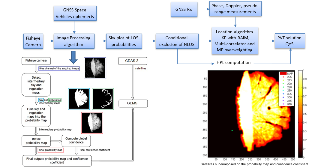
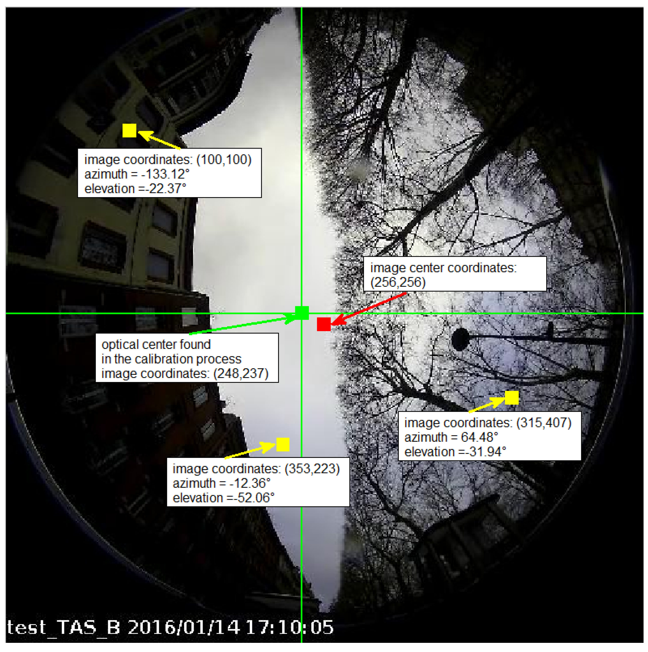
The role of the image processing module is the segmentation of each image forming the sequence of images acquired by the fisheye camera, indicating if a pixel belongs to the sky or to an object (obstacle) which disrupts the LoS towards a satellite. In order to increase the viability of the information extracted by the image processing module, our choice of output is the probability map of a pixel corresponding to a satellite in LoS. The image processing module needs also to compute the correspondence between an image pixel and a couple of elevation and azimuth angles. Having the sky/non-sky segmentation and the correspondence elevation, azimuth-image pixel, the localization module will be able to decide if a satellite (also named Space Vehicle, SV), having the elevation and azimuth known, is in LoS or NLoS, and hence adopt a proper localization approach. The correspondence between elevation, azimuth and an image pixel is obtained by performing camera calibration [5,6]. An example of computed correspondence using the toolbox provided by the authors of [5,6] is given in Figure 1. The calibration process performs the projection of the image on a hemisphere. Once this projection is known, we have the azimuth and elevation for each pixel. The elevation is given by the z-coordinate of the pixel and the azimuth is the angle between the x-axis and the projection on the (x,y) plane of the pixel. Thus, the azimuth is computed based on x and y coordinates. All these computations are made with respect to the optical center found in the calibration process.
Next, the proposed algorithm produces the probability map, which represents the output of the image processing module. Using the information provided by the GNSS receiver, the surrounding satellites are marked on the probability map. A three-levels discretization of LoS probability map has been considered. Its result is the rejection of the satellites in NLoS and the weighting of satellites with small probabilities. Next, the GNSS data corresponding to remaining satellites go through the Kalman filter (belonging to the GNSS receiver) correction step, which provides the final Position, Velocity, Time (PVT) solution. The Horizontal Protection Level (HPL) can be computed from the output of the Kalman filter, facilitating the computation of the Horizontal Positioning Error (HPE) and Miss-Integrity (MI), which is selected as a QoS indicator. The HPL is defined as the radius of a circle in the horizontal plane, with its center being at the true position, which describes the region assured to contain the indicated horizontal position.
The horizontal positioning errors are computed based on the position error in the north (parallel with the ordinates’ axis) and the east (parallel with the abscissas’ axis) components. These errors are computed based on the difference between measured positions and referenced true positions:
where:
due to the bi-dimensional nature of the horizontal error. The HPE can be represented as a radial error:
The effect of the DOP on the horizontal position value is evaluated with the aid of the Horizontal DOP (HDOP) indicator.
Navigation system integrity refers to the ability of the system to provide timely warnings to users when the system should not be used for navigation. The evaluation of integrity is achieved by means of the concepts of Alert Limit, Integrity Risk, Protection Level and Time to Alert, explained in the following.
- Alert Limit (AL): The alert limit for a given parameter measurement is the error tolerance not to be exceeded without issuing an alert. The horizontal alert limit is the maximum allowable horizontal positioning error beyond which the system should be declared unavailable for the intended application.
- Time to Alert (TA): The maximum allowable time elapsed from the onset of the navigation system being out of tolerance until the equipment enunciates the alert.
- Integrity Risk (IR): The probability that, at any moment, the position error exceeds the Alert Limit.
- Protection Level (PL): Statistical bound error computed so as to guarantee that the probability of the absolute position error exceeding said number is smaller than or equal to the target integrity risk. The horizontal protection level provides a bound on the horizontal positioning error with a probability derived from the integrity requirement.
Based on IR and PL values, MI can be estimated. There are two integrity monitoring methods: Receiver Autonomous Integrity Monitoring (RAIM) and receiver assisted by ground monitoring stations, namely Satellite-Based Augmentation Systems (SBAS) or Ground-Based Augmentation Systems (GBAS). We will use in the following a RAIM system to estimate the integrity indicators.
The camera aiding algorithm proposed in this paper is as follows:
- The GNSS pseudoranges and pseudorange rates are computed with the software receiver GNSS Environment Monitoring Station (GEMS) [7] using the Multi-Correlator (MC) tracking loop with the multipath detection activated.
- These measurements are fed into the EKF prediction step and the associated Receiver Autonomous Integrity Monitoring (RAIM) can thus exclude faulty satellites.
- For each satellite left, the elevation and the azimuth are computed and projected onto the camera reference frame using the vehicle heading computed from the reference trajectory. In an operational mode, the heading would be computed from the GNSS velocity. For our experiments, it is computed from the reference trajectory, so there is no error on the projection of the satellites on the camera reference frame and then the best possible contribution of the camera aiding can be assessed.
- A three-levels discretization of LoS probability map has been considered:
- ⚬
- LoS level: When the probability to be in LoS (pLoS) is between 0.75 and 1, the received signal is considered as the LoS, and the measurements are kept unchanged.
- ⚬
- Doubt level: When the pLoS is between 0.25 and 0.75 (most likely related to building edges or vegetation), there is doubt on the quality of the received signal, so an overweighting is applied on the measurements as:where el is the elevation angle, f is a factor set to 2 (corresponding to the number of extra street crossings of the multipath with respect to the LoS) and L is the average width of the street, which is set to 10 m.
- ⚬
- NLoS level: Finally, when pLoS is between 0 and 0.25, the received signal is considered as NLoS and the measurements are excluded if there are enough LoS space vehicles; otherwise, they are kept and overweighted as above.
- The remaining GNSS data go through the Kalman filter correction step, which provides the final PVT solution.
- The Horizontal Protection Level (HPL) is computed from the output of the Kalman filter.
- The Horizontal Positioning Error (HPE) and Miss-Integrity (MI) are computed from the output of the Kalman filter and the reference trajectory.
While several papers have already addressed the hybridization techniques between GNSS and inertial sensors [2,3], the hybridization between the camera and GNSS seems to have been less researched. However, this technique appears very promising, especially today, as camera and GNSS receivers have become nominal equipment of any terminal. The significance of our approach consists in the complete analysis of the solution proposed, starting from the design, continuing with the experimental validation and finishing with the estimation of the QoS indicator. The results obtained are encouraging, recommending the utilization of the approach proposed for GNSS localization in constraint environments.
We present in the following the principal materials and methods used in our research, following the steps of the camera aiding algorithm already presented.
2.1. Data Acquisition
The first step of the proposed camera-aided algorithm is data acquisition. For image acquisition, we have selected a fisheye camera model VIVOTEK FE8181/81V with 180° panoramic view and 360° surround view. This choice was made because we need an acquisition device capable of seeing the entire sky-related scene. The GNSS pseudoranges (acquired by any GNSS receiver, such as the one mounted on the vehicle carrying the fisheye camera) and pseudorange rates are computed with the software receiver GEMS [7] using the MC tracking loop with the multipath detection activated. The second step of the camera-aided algorithm supposes the transmission of these measurements into the EKF prediction step, and thus the associated RAIM can exclude faulty satellites. This step ensures the functioning of the proposed system in normal propagation conditions.
2.2. Image Processing Module
For the third step of the camera-aided algorithm presented in the Introduction, which supposes the projection of the surrounding satellites’ coordinates onto the camera reference frame using the vehicle heading computed from the reference trajectory, the image processing module is needed. It transforms each image acquired by the fisheye camera into a probability map. The first step of the algorithm which implements the image processing module is the segmentation of each image.
2.2.1. Image Segmentation
The segmentation task is one of the most difficult tasks in image processing. A great variety of approaches for segmentation are proposed in the literature. Image segmentation aims at partitioning the image into a number of non-overlapping regions, named segments. Ideally, each segment corresponds to an image object or a meaningful part of an object. Mainly, there are two classes of image segmentation approaches. Low-level image processing methods address only the problem of partitioning the image into a number of homogeneous regions. The goal of these methods is to minimize the number of regions, while keeping them homogeneous. The second class of approaches is represented by higher-level image segmentation methods, which address object segmentation. Generally, these objects appear as homogeneous regions in images. The higher-level image segmentation methods are often called semantic segmentation, or image parsing. Object segmentation is most successful in applications with restricted image variability or content. From a mathematical point of view, the general problem of image segmentation is an ill-posed problem [8], meaning that there is no unique solution and that the segmentation problem is task-dependent. The main problems with the existing algorithms for sky segmentation are erroneous detection of sky areas with large ranges of color, false detection of sky reflections or other blue objects and inconsistent detection of small sky areas. Blue sky segmentation for image editing is addressed in [9]. The initial sky probability is modeled as a product of color, position and texture probabilities. After the first sky segmentation is obtained, with the probabilistic model defined, the sky model parameters are re-estimated, from the sky region, to obtain an adaptive model. The adaptive model appends a new feature, defining a sky confidence measure, to the already defined color, position and texture probabilities. This adaptive model is used to obtain the final sky segmentation.
Excellent results are obtained for clear skies, as assumed by the authors of [9]. A two-step method for sky detection is proposed in [10]. In the first stage, a region-based segmentation, the Color Structure Code (CSC) [11], is used to generate a number of segments. In the second stage, segments are classified to the sky or to the non-sky class, according to simple yet powerful heuristics. Closer to our approach is the work presented in [12,13], meaning that real time constraints are taken into account. The authors of [12,13] conclude that a strategy based on simplification by geodesic reconstruction using dilatation coupled with a classification with Fisher’s algorithm and a post-treatment gives the best compromise between quality of results and computational time. The aim of the simplification stage is to smooth the uniform regions of images, making the classification step easier. Therefore, the simplification filter is a smoothing filter which does not affect very much the edges of the image processed.
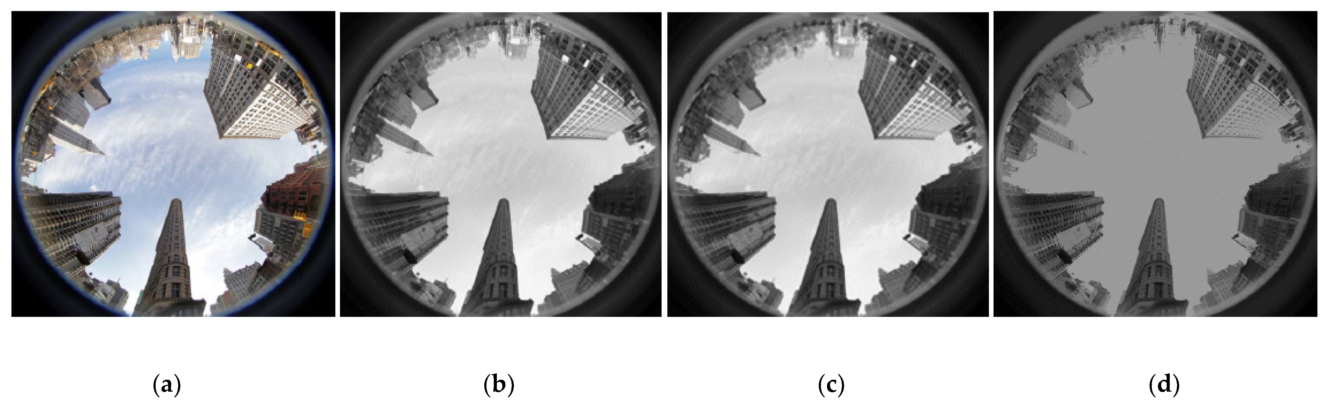
A better choice for the simplification filter concerning the quality of segmentation is proposed in [14]. This approach is based on the remark that the images of Brownian fields (characterized by some values of the Hurst exponent, H) are similar to the images of sky [15]. By estimating the local Hurst exponent in an image, we can localize the sky regions as areas with constant H. The proposal in [14] is to simplify the image content by a denoising filter that uses regularized Hurst estimation, proposed in [16]. The estimation of the Hurst parameter, which models the texture content in the image, is done using a generalized LASSO approach. For comparison purposes, the authors of [14] used the Ordinary Least Squares (OLS) regression from [17] as well. The OLS-based and LASSO-based filters used in [14] remove details from the finest resolution levels of the Dual Tree Complex Wavelet Transform (DTCWT) [18], without degrading the image edges and hence the quality of the segmentation. A simple classifier is used in [14] after the simplification filter, which requires as input only the number of clusters, namely the k-means classifier. In Figure 2 is shown a comparison of the results obtained by applying the segmentation methods proposed in [13] and [14] on the image in [19]. This is one of the most complicated images which can be delivered by a fisheye camera in practice. We can remark, comparing visually the images in the panels from Figure 2b–d, that the simplification filters proposed in [14] preserve better the details of the border region between sky and non-sky regions than the simplification filter proposed in [12,13], affecting the edges less. Using the simplification filters proposed in [14], we observe, comparing panels from Figure 2f–h, an improvement in the separation of building/sky versus the result obtained by applying the simplification filter in [12,13].
In these panels, the regions classified as non-sky are marked in black. LASSO slightly outperforms OLS. In the case of the segmentation method proposed in [12,13], whose result is shown in panel (h), we observe areas in the building where the classifier decides that the building is part of the sky cluster (these areas are not marked in black). The running time of the segmentation method proposed in [14] is longer than the running time of the segmentation method proposed in [12,13].
The segmentation algorithm selected for the present paper uses the blue channel of the acquired image and the segmentation is performed by using the geodesic reconstruction using the dilatation simplification filter [12,13] associated with the k-medoid classification algorithm [20]. The related literature [12,13,14] showed that using the k-means algorithm in order to segment the sky regions gives very good results. Our choice for the k-medoid algorithm is based on the fact that, generally, the k-medoid yields better results than the k-means algorithm when dealing with a segmentation task. The result of the segmentation step is a binary sky map. The segmentation approach was extensively tested on hundreds of fisheye camera images and the estimated accuracy is around 97.87%. Various weather conditions were considered: sunny, cloudy and light rain. However, considering only heavy rain weather conditions, the accuracy drops to 81.28%, due to rain drops that corrupt the image seen by the camera.
2.2.2. Image Processing Module Block Diagram
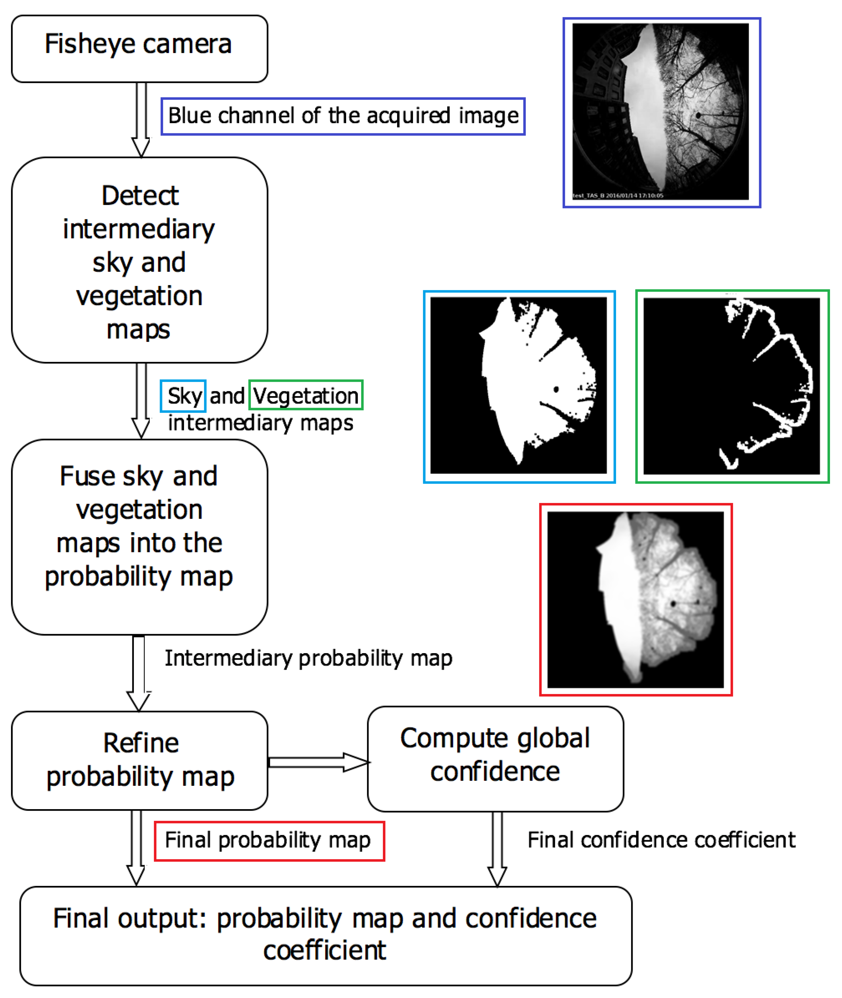
The image processing module general block diagram is presented in Figure 3. The function of this module is to identify clear sky regions, vegetation regions and to generate a LoS probability map for each image acquired. The first step of the algorithm which implements the image processing module is the segmentation described in the previous sub-section. Using edges and curvature information of the image edges, the vegetation map is constructed as well. Both these maps, sky and vegetation, are then fused to produce the intermediary probability map, using the three-levels discretization, which represents the fourth step of the camera aiding algorithm presented at the end of the Introduction. The final sky probability map is obtained after a refinement that takes into account the position uncertainty of the satellites in the image. Basically, a low-pass filter is used in order to blur the probabilities around the vegetation-related edges and also for the buildings, but to a smaller degree.
Next, the fifth step of the camera-aided algorithm is realized. The remaining GNSS data go through the Kalman filter correction step, which provides the final PVT solution.
2.3. GNSS Signal Processing
Integrity determination techniques that allow providing a QoS indicator to the user have been studied for decades. The quality indicator can be defined as a PL provided together with the position. State of the art techniques that cover algorithms able to detect and identify faulty measurements are documented in several papers [21,22,23,24]. Standard RAIM [25] has been initially designed for civil aviation. Its use for ground applications has been widely studied these last few years, with always a strong limitation found in the definition of nominal and threat models, as well as the setup of the probability of occurrence of the threats [26]. As a consequence, RAIM application to ground users often results in large PLs or high MIs due to the inadequate over bounding of local effects in the nominal model. Focusing on the land application use case, ref. [27] proposed a new methodology to provide with PVT QoS characterization better than what can be currently achieved with the aforementioned techniques. To this end, the multiple GNSS constellations, the multiple frequencies, as well as the Key Performance Indicator (KPI) elaborated along the signal processing chain of a GNSS receiver were considered. In particular, in order to detect multipath and mitigate the induced pseudorange error, MC maximum likelihood discriminator [28] is used. In addition to the induced error mitigation, as soon as a multipath is detected, the corresponding measurements are overweighted in the Position, Velocity, Time + Integrity (PVT + I) computation. Figure 4 illustrates the PVT horizontal error using the EKF algorithm in [27] and several code tracking discriminators. White dots represent a simple Early-Minus-Late Power (EMLP) discriminator, blue dots represent the MC when the multipath detection is not activated and, finally, green dots represent the MC when the multipath detection is activated.
The improvement in the positioning accuracy is clearly visible in this example. However, short NLoS are still an issue and might cause biased positioning and missed integrities. In this case, the camera is expected to allow the identification of NLoS situations. The final steps of the camera-aided algorithm proposed in the Introduction permit the evaluation of its performance. First is computed the HPL using the output of the Kalman filter; next is computed the HPE and, finally, MI is computed using data from the output of the Kalman filter and the reference trajectory.
3. Results and Discussion
We have simulated the camera-aided algorithm proposed and we have compared the results obtained using the same data in two cases, with and without the utilization of this algorithm. An experimental campaign was organized to accomplish this objective.
3.1. Experimental Campaign
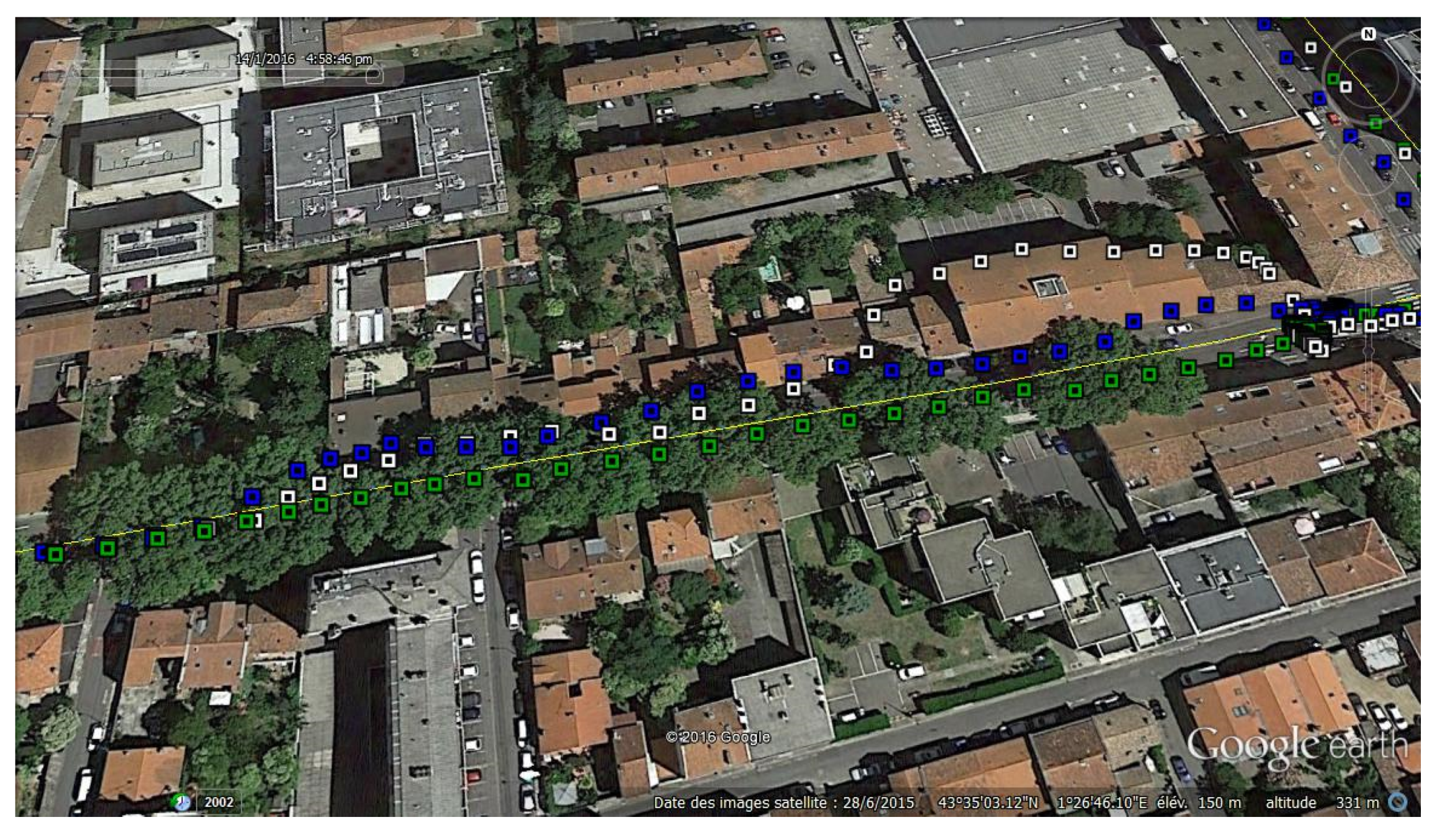
The goal of the field trials campaign is to assess the camera contribution to the improvement of a PVT solution computation and to validate the fusing algorithm. The experimental configuration is illustrated in the right-hand part of Figure 5. The data collecting system consists of:
- Fisheye camera;
- GNSS Data Acquisition System (GDAS-2) used to capture and record GNSS raw signals;
- The live-sky testing platform, including the car carrying the equipment, was provided by GNSS Usage Innovation and Development of Excellence (GUIDE), a Toulousian test laboratory. It embeds a GBOX that provides the reference trajectory based on high-grade INS and GNSS differential corrections from the International GNSS Service (IGS).
The reference trajectory is then compared to the corrected trajectory obtained by computing the car’s positions with the proposed algorithm, to calculate the positioning error and evaluate the integrity of the proposed navigation algorithm.
The campaign was organized on January 2016 in Toulouse on the itinerary shown in the left-hand part of Figure 5. The main trajectory lasted 1800 s in an urban environment and involved 18 satellites from three constellations (8 GPS; 2 Galileo; 8 GLONASS), among which a maximum of 12 satellites were used simultaneously in the PVT.
3.2. Global Results
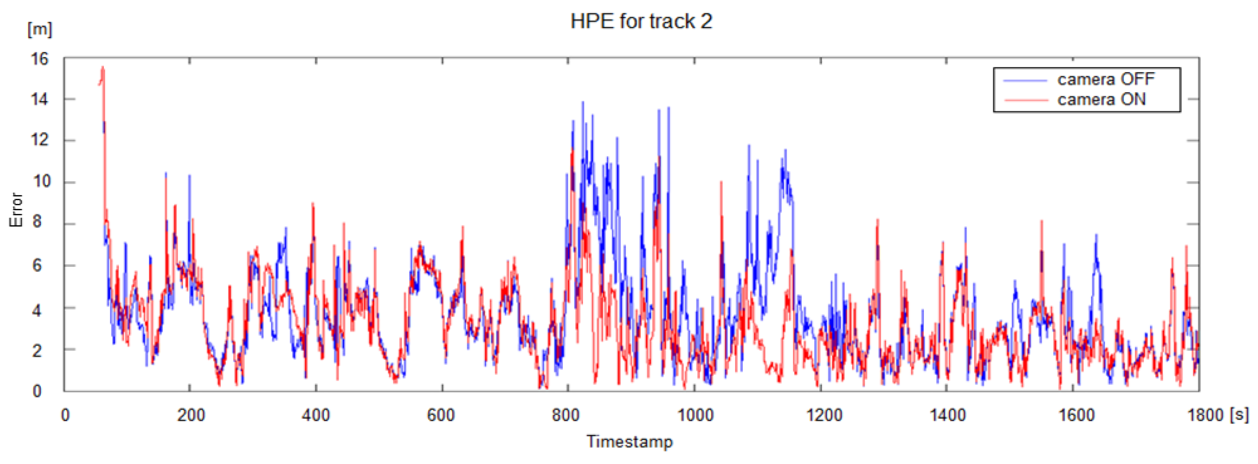
Figure 6 illustrates the HPE on the whole track in both situations: with camera ON (in red) and with camera OFF (in blue). Table 1 summarizes the performance of the PVT algorithm in terms of accuracy, protection levels and integrity.
For HPE and HPL, we considered in Table 1 three situations corresponding to three time intervals: 67%, 95% and 99% of whole recording’s duration. Analyzing Figure 6, it can be noted that the camera makes it possible to improve the positioning accuracy whatever the time percentages (67%, 95% or 99%) because the red curve is under the blue curve almost all the time (except right at the beginning of the trajectory). This remark is in agreement with Table 1, where the HPE values corresponding to the case when the camera is on are inferior to the values of HPE obtained when the camera is off for all three time intervals. However, we observe, by analyzing Table 1, that the HPL are increased by around 15% for 67% and 95% of the time and by around 30% for 99% of the time. This HPL increase is mainly due to DOP degradation, which appears as a consequence of satellite exclusion and to measurement overweighting.
It can also be seen from Figure 6 that several sections where the camera improves the accuracy can clearly be identified. One of these sections has been selected to be more deeply analyzed in the following sub-section.
3.3. Discussion
In the following, we discuss the results and how they can be interpreted from the perspective of working hypotheses.
3.3.1. Focus on an Area Where the Camera Aiding Algorithm Improves the PVT
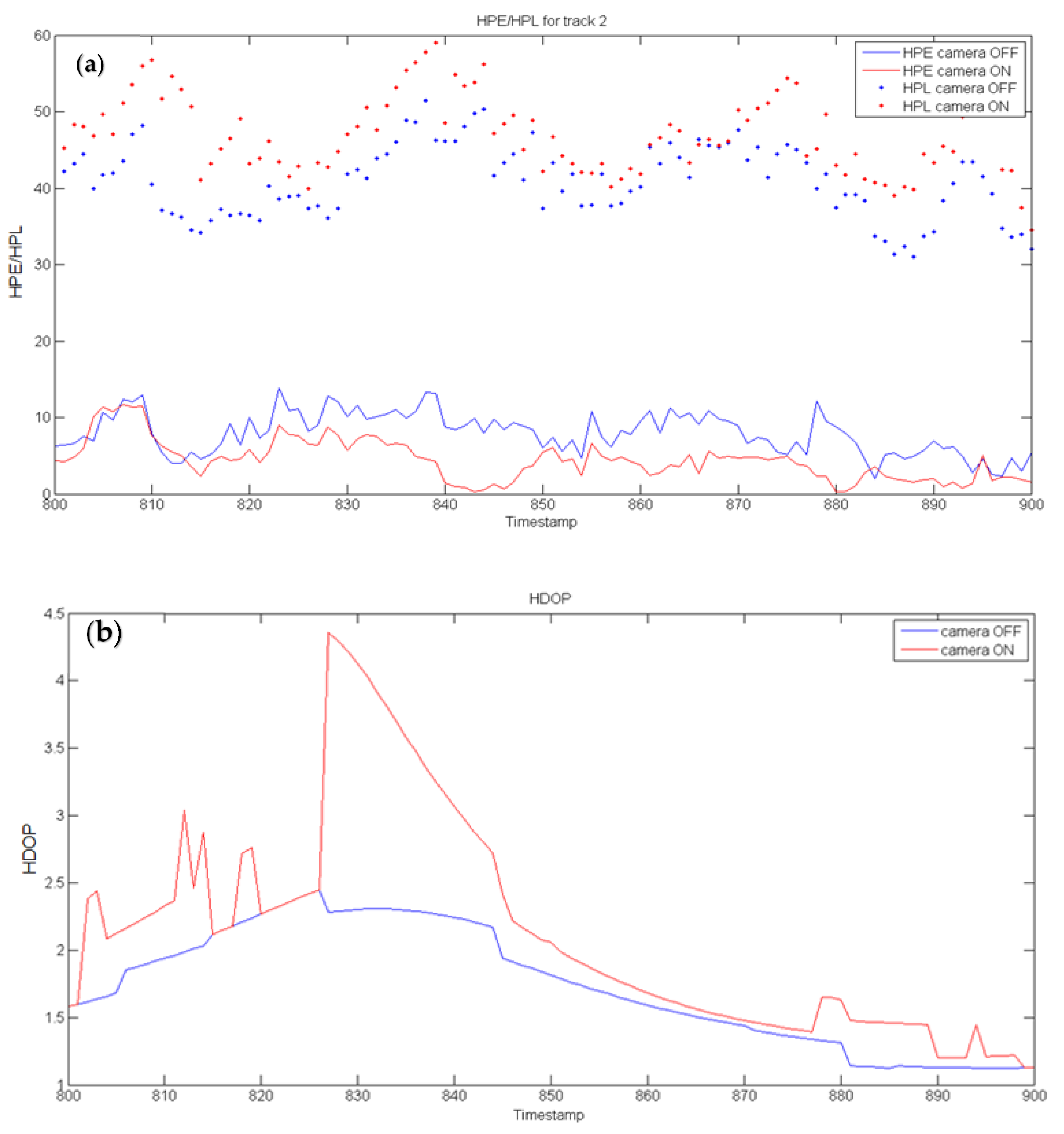
Figure 7 evidences the HPE improvement around time stamp 850. In this area, the mean error without the camera is around 8 m while it is less than 4 m when the camera is used.
The proposed experimental setting (shown in Figure 5) enables us to correlate the HPE with HPL, HDOP and the number of satellites used in the PVT. It can be observed on the upper panel in Figure 8 that the HPE improvement is associated with the HPL increase. The PL increase is due to satellite exclusions and HDOP increases.
However, due to the Kalman filtering effect, the HDOP fluctuations are neither totally nor instantaneously reported on the HPL fluctuations. On the contrary, it can be checked that satellite exclusions do instantaneously impact the HDOP. At timestamp 861, only one satellite is excluded, as can be observed in Figure 9. Compared to the case in which the camera was not used, this leads to an increase of HDOP and consequently to an increase of HPL (see Figure 8). However, this also leads to an improvement in accuracy (see Figure 7) by more than 8.5 m.
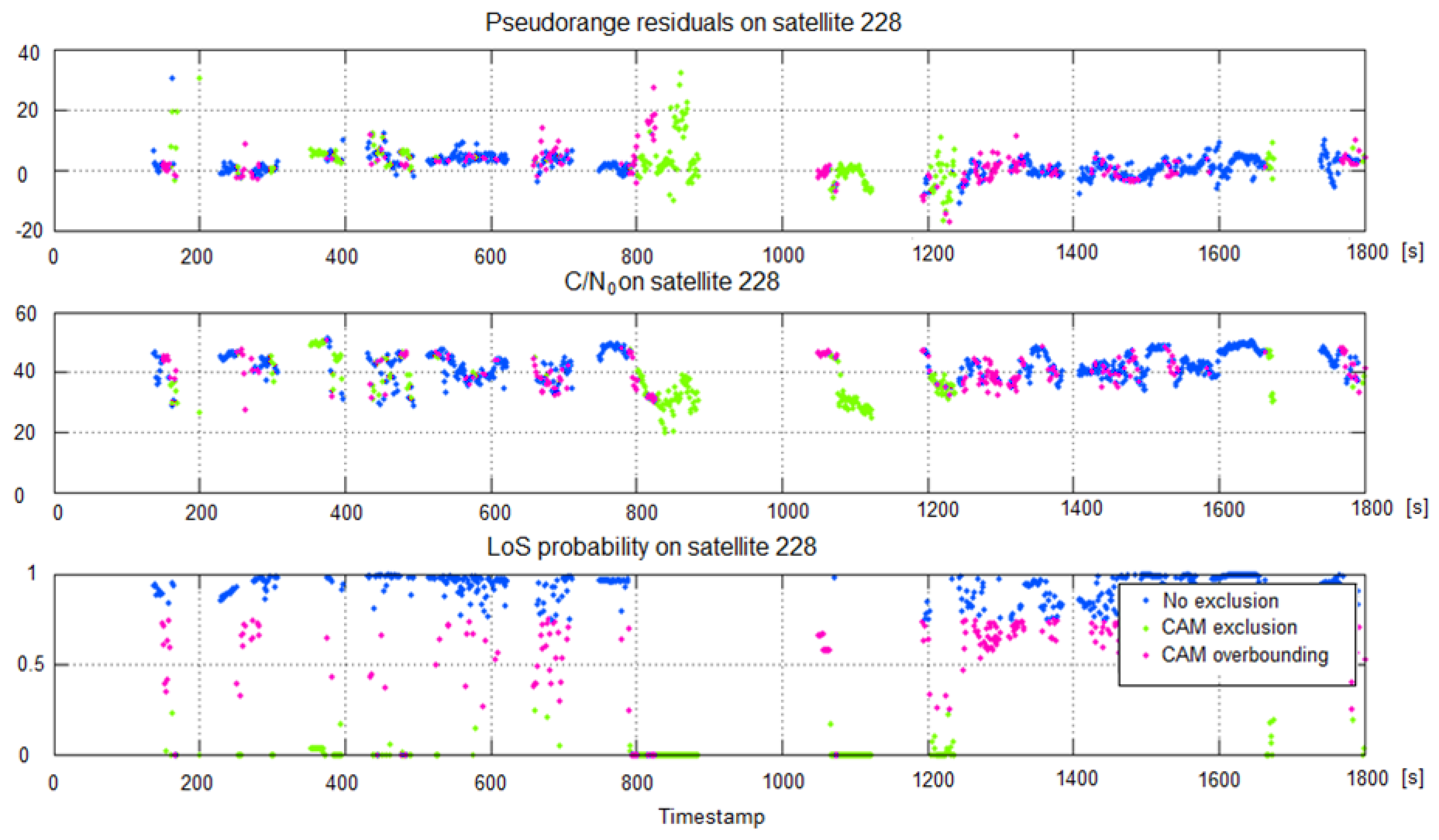
Figure 9 represents the physical context at timestamp 861. On one side of the road, a high building can be seen, and on the other side, trees are observed. Figure 9 confirms that only one satellite (ID 228, i.e., GPS 28) is to be excluded as it is masked by the building. Finally, Figure 10 illustrates the pseudorange residuals, the Carrier to Noise ratio (C/N0) and pLoS for the GPS PRN 28. Focusing around timestamp 861, it can be confirmed that the C/N0 is strong enough to track the satellite; however, the measurements are biased by around 32 m. In this case, the camera exclusion significantly improves the HPE and the DOP degradation is weak.
A few seconds later, a street lamp pole “hides” the satellite 213 and thus it is declared as NLoS and is excluded from the PVT. Nevertheless, although not illustrated here, the GNSS data were perfectly valid for this timestamp (pseudorange are not biased and C/N0 very good). This corresponds to a typical case where the camera exclusion should not be trusted.
3.3.2. Statistic on Pseudorange Residuals
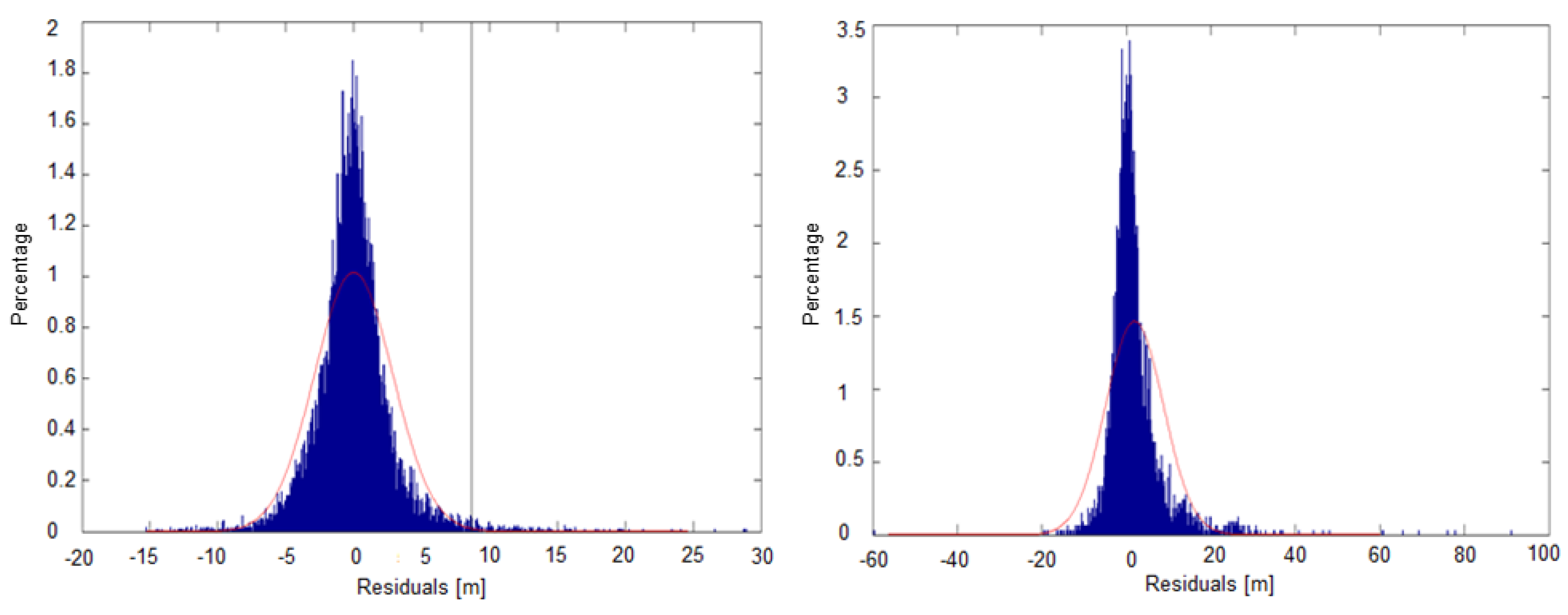
This last sub-section no longer proposes a focus on a specific area but proposes a statistic on pseudorange residuals in order to assess the statistics of NLoS occurrence and impact in urban areas. The red line in the left-hand part of Figure 11 represents the probability density function (pdf) of the pseudorange residuals marked as LoS by the camera, and the red line in the right-hand part of Figure 11 represents the pdf of the pseudorange residuals marked as NLoS by the camera. All these residuals are computed from the EKF PVT. Both pdfs represented by red lines in Figure 11 are obtained by fitting the corresponding histograms represented in blue in Figure 11. In clear sky conditions and thermal noise only, the pseudorange residuals’ distribution should be Gaussian. The pdf in the left-hand part of Figure 11 looks Gaussian or at least symmetrical, tending to indicate that for those data, the MC processor was able to remove the multipath components. However, the distribution on the right-hand part is clearly asymmetric.
The residuals larger than 8.6 m (3σ of the “clean” distribution, represented by a vertical line on the left panel in Figure 11) are considered to be due to NLoS conditions. They represent around 2% of the whole distribution. Moreover, 70% of these residuals are marked as NLoS by the camera, and 100% of the residuals greater than 29 m are marked as NLoS by the camera, which represents 0.13% of the measurements.
Areas for improvement may exist both regarding the image processing and the GNSS processing:
- Propose a criterion or a set of criteria in order to decide which data to exclude or to overweight in case the camera flags too many data as NLoS;
- Detect small and close “obstacles” (such as lamp poles) in order not to mark the related area as NLoS;
- Improve classification of vegetation;
- Feedback loop and additional criteria for adaptively tuning the image processing parameters regarding the threshold used on the probability map.
4. Conclusions
The real signal tests show that the camera clearly brings some improvements in the situations where NLoS signal is present but not detected by the EKF RAIM. The contribution brought by the camera allowed to reduce the HPE distribution, while only slightly increasing the HPL (less than 15% degradation, at least up to the 95th percentile, mainly due to the DOP degradation), and very few areas remain where the camera degrades the positioning accuracy.
Although not illustrated here, it also appeared that the “three-levels” discretization of the LoS probability map is beneficial with respect to a binary discretization, as it allows considering building edges as “doubtful” areas. At least two reasons have been evidenced for the position degradation:
- Effect of small obstacles such as lamp poles that cause a NLoS flag by the camera while not significantly affecting the quality of the data;
- Difficult classification of the vegetation that can be considered a wrong source of NLoS, leading to the exclusion of too many measurements.
The problem with the small objects that appear to block the satellite data will be treated in the future by integrating context into the classification. At this point, our classifier works at pixel level. Moreover, some morphological operations could refine the response. For the second disadvantage, concerning the classification of the vegetation, we envisage the use of new, more performant classifiers such as neural networks.
Author Contributions
Conceptualization, A.C. and M.M.; methodology, C.D. and G.C.; software, C.D., C.N. and G.C.; validation, C.D., C.N. and G.C.; formal analysis, V.G. and A.C.; investigation, C.D. and G.C.; resources, A.C. and M.M.; data curation, G.C.; writing—original draft preparation, C.D., C.N., G.C.; writing—review and editing, C.D. and C.N.; visualization, C.D. and G.C.; supervision, V.G., A.C. and M.M; project administration, A.C. and M.M.; funding acquisition, A.C. and M.M. All authors have read and agreed to the published version of the manuscript.
Funding
This research was funded by the European Space Agency with ESA Contract No. 4000111852/14/NL/CBi (Quality of Services Improvement for GNSS Localisation in Constraint Environment by Image Fusing Techniques (IMFUSING)) with Politehnica University, Timisoara, Romania.
Institutional Review Board Statement
Not applicable.
Informed Consent Statement
Not applicable.
Data Availability Statement
Not applicable.
Conflicts of Interest
The authors declare no conflict of interest.
Appendix A. GNSS Basics
The GNSS architecture contains three blocks: the acquisition sub-system, the tracking sub-system and the navigation sub-system. The roles of these sub-systems are the following.
Acquisition:
- to detect the GNSS signals which are present;
- to realize a first estimation of their frequency and delay characteristics.
Tracking:
- to rest locked on the signals received from the acquisition sub-system;
- to decode the navigation message;
- to estimate the distance traveled by each signal to arrive at the receiver.
Navigation:
- to calculate the position of the receiver;
- to determine the bias of the receiver’s internal clock versus the reference system.
The estimation of the position of the vehicle which carries the GNSS receiver is done by triangulation in the navigation sub-system. The distance between the receiver’s carrier vehicle and each satellite available in the region where the vehicle is situated is estimated in the tracking sub-system, and based on these estimations, the localization is made. The position estimation accuracy depends on the number of satellites available, on their positions and on the quality of the signals received from these satellites. The distance towards the satellite (range) can be estimated by the tracking sub-system of the GNSS receiver with the aid of the delay, τ, between the emission of the incident wave and the reception of the reflected wave. The access to GPS satellites is provided by the Code Division Multiple Access (CDMA) principle. Each satellite has its own Pseudo Random Noise (PRN) code, which is a bipolar signal, C(t). It is multiplied with the data transmitted by the satellite for navigation purposes, D(t), obtaining a new bipolar signal, which represents the modulator for the Binary Phase Shift Keying (BPSK) modulation of the carrier. The power of the transmitted signal is denoted by Ec. The expression of the signal generated is:
This is a very large bandwidth signal. The received signal is of the form:
where the delay (proportional to the target range) is denoted by τ0, the Doppler frequency (related to the target velocity) by ν0, η(t) represents a complex white Gaussian noise with power spectral density N0 and b is a random variable which describes the propagation. In modern implementations, such as for several GALILEO signals, the BPSK modulation is replaced by Binary Offset Carrier (BOC) modulation. This BOC modulation, along with their modified versions multiplexed BOC (MBOC) and composite BOC (CBOC), uses a sub-carrier to create separate spectra on each side of the transmitted carrier. It presents some advantages, such as a high degree of spectral separation from existing navigation signals, and leads to significant improvements in terms of tracking, interference and multipath mitigation.
The GNSS signal is detected by the acquisition sub-system with the aid of a Maximum Likelihood (ML) detector, by correlation with a locally generated replica. The sampled version of the received signal, s[n], is multiplied with a sampled version of the signal c(t), locally generated, c[n], which is delayed with a delay τ, taken from a lookup table, and is multiplied with a complex exponential with argument ν taken from the same lookup table. The N samples of the multiplication’s result are added, obtaining a sufficient statistic, T(s) (proportional with the correlation of signals s[n] and c[n], computed in zero), whose value is compared with a detection threshold, γ’. If the value of T(s) is bigger than the threshold value, then the hypothesis H1 which supposes that τ0 = τ and that ν0 = ν will be considered as true. Otherwise, other values for τ and ν will be selected from the lookup table and the computation procedure, already described, will be repeated. Thus, both parameters, range and radial velocity, are estimated simultaneously, by a search in the range (delay)–velocity (Doppler frequency) plane. To perform this first search of Doppler frequency and of delay, the acquisition sub-system of the GNSS receiver uses a frequency and delay lookup table to find the correlation peak. If the incoming signal is affected by thermal noise or/and multipath propagation, the output of the coherent correlator will be affected as well. The best Maximum Likelihood (ML) estimation of the range and relative velocity of the satellite can be obtained as:
where ν is the Doppler frequency and represents the cross-ambiguity function of the signals s(t) and c(t), defined as:
The cross-ambiguity function is a time–frequency representation which has a wide utilization in target localization problems, such as in radar, sonar, GPS and so on. In simple scenarios, without multipath propagation, such as in the case of a car travelling in a plain rural region, the satellite is in Line-of-Sight (LoS) and the received signal has the expression in (2) with b = 1.
In more complicated scenarios, such as in natural or urban canyons, reflections from (possibly moving) objects in the surroundings produce multipath propagation, whose effect is the multipath fading. The Cramer–Rao theorem specifies the conditions for an unbiased estimator of a single parameter, θ, of a data set x, f(x), to have minimum variance and to be efficient. The theorem specifies the value of this minimum variance as well. This value represents a lower bound for all the unbiased estimators of the considered parameter and is named the Cramer–Rao Lower Bound (CRLB). The unbiased estimator which has this variance, f(x), is named the optimal estimator. Its expression can be deduced by solving the equation:
where p(x;θ) represents the data probability density function dependent on the parameter θ and I(θ) represents the Fisher information. In the following, we will consider the delay as parameter, θ = τ and we will present the expressions of the CRLB for GNSS delay estimation in cases without and with Non-Line-of-Sight (NLoS) multipath propagation. In the first case, the signal model is:
The corresponding Cramer–Rao Lower Bound has the expression [29]:
where SNR represents the signal-to-noise ratio, defined as 2Ec/N0, and represents the square of the effective bandwidth of the transmitted signal c(t), defined as:
Therefore, in the case when there is no multipath propagation, and the satellite is in LoS, the CRLB varies inverse proportionally with the square of effective bandwidth of the transmitted signal σf and with the signal-to-noise ratio of the received signal, SNR. The range estimation precision increases with the decreasing of the CRLBwithout multipath. This explains why GNSS designers have chosen the CDMA modulation, which has a large effective bandwidth. The single impairment which affects the precision of range estimation in the case of propagation without multipath is the receiver’s thermal noise, whose power spectral density decreases the SNR.
In the second case, when the propagation is affected by multipath and the satellite is NLoS, we use the signal model in (A2), considering that the random variable b is a zero-mean, complex Gaussian random variable, with variance , and the expression of the CRLB for the delay estimation is:
where:
Therefore, in this case, the CRLB depends on the effective bandwidth of the transmitted signal σf and on the signal-to-noise ratio, SNR, as in the first case, but also on the variance of the NLoS multipath fading . Numerical simulations prove that the NLoS multipath propagation can deteriorate more than 100 times the precision of localization.
In the case of real-life GNSS signals, the correlation peak detected in the acquisition sub-system fluctuates at each time instant. Because an error of 1 ms in the code delay produces an error of around 300 km in pseudorange, the tracking sub-system is necessary. The tracking sub-system is composed of a set of loops permitting the tracking of signals which were detected. The Delay Lock Loop (DLL) is in charge of the delay’s tracking. Based on multiple correlators, it estimates the delay between the received signal and the locally generated replica. Knowing in this way the code phases at the moment when the signal was sent by the satellite and at the moment when the signal was received, the tracking sub-system finds the signal flying time. This time is then transformed into a pseudorange measure by multiplication with the speed of light. The role of the Frequency Lock Loop (FLL) is to maintain a good estimation of the received signal frequency. The measurement of the carrier phase (Phase Lock Loop-PLL) permits the pseudorange estimation with a better precision, but its utilization is delicate (2π-ambiguity). Using the pseudorange measures realized by the tracking sub-system, the navigation sub-system computes the receiver position using the principle of triangulation. Position calculations involve range differences, and where the ranges are nearly equal, small relative errors are greatly magnified in the difference. This effect, brought about as a result of satellite geometry (the range differences are small if the satellites used for triangulation are close to each other), is known as Dilution of Precision (DOP). The position measurement errors require the utilization of filters able to weight the measurements in function of the confidence granted. The most used algorithm is the Kalman filter or one of its variants, such as the Extended Kalman filter (EKF).
References
- ETSI. Technical Report ETSI TR 101 593. ETSI Satellite Earth Stations and Systems (SES); Global Navigation Satellite System (GNSS) Based Location Systems, Minimum Performance and Features; V1.1.1; ETSI: Sophia Antipolis, France, 2012. [Google Scholar]
- Zhang, H.; Li, W.; Qian, C.; Li, B. A Real Time Localization System for Vehicles Using Terrain-Based Time Series Subsequence Matching. Remote Sens. 2020, 12, 2607. [Google Scholar] [CrossRef]
- Li, N.; Guan, L.; Gao, Y.; Du, S.; Wu, M.; Guang, X.; Cong, X. Indoor and Outdoor Low-Cost Seamless Integrated Navigation System Based on the Integration of INS/GNSS/LIDAR System. Remote Sens. 2020, 12, 3271. [Google Scholar] [CrossRef]
- Bovik, A. (Ed.) Handbook of Image & Video Processing; Academic Press: San Diego, CA, USA, 2000. [Google Scholar]
- Scaramuzza, D.; Martinelli, A.; Siegwart, R. A flexible technique for accurate omnidirectional camera calibration and structure from motion. In Proceedings of the Fourth IEEE International Conference on Computer Vision Systems (ICVS’06), New York, NY, USA, 4–7 January 2006; p. 45. [Google Scholar]
- Scaramuzza, D.; Martinelli, A.; Siegwart, R. A Toolbox for easily calibrating omnidirectional cameras. In Proceedings of the 2006 IEEE/RSJ International Conference on Intelligent Robots and Systems, Beijing, China, 9–15 October 2006; pp. 5695–5701. [Google Scholar]
- Kubrak, D.; Carrie, G.; Serant, D. GNSS Environment Monitoring Station (GEMS): A real time software multi constellation, multi frequency signal monitoring system. In Proceedings of the International Symposium on GNSS, ISGNSS, Jeju, Korea, 21–24 October 2014. [Google Scholar]
- Béréziat, D.; Herlin, I. Solving ill-posed Image Processing problems using Data Assimilation. Numer. Algorithms 2010, 56, 219–252. [Google Scholar] [CrossRef] [Green Version]
- Zafarifar, B.; de With, P.H.N. Adaptive modeling of sky for video processing and coding applications. In Proceedings of the 27th Symposium on Information Theory in the Benelux, Noordwijk, The Netherlands, 8–9 June 2006; pp. 31–38. [Google Scholar]
- Schmitt, F.; Priese, L. Sky detection In Csc-segmented color images. In Proceedings of the 13th International Joint Conference on Computer Vision, Imaging and Computer Graphics Theory and Applications; SCITEPRESS Science and Technology Publications: Setúbal, Portugal, 2009; pp. 101–106. [Google Scholar]
- Rehrmann, V.; Priese, L. Fast and robust Segmentation of natural color scenes. In Proceedings of the Transactions on Petri Nets and Other Models of Concurrency XV; Springer: Berlin/Heidelberg, Germany, 1997; pp. 598–606. [Google Scholar]
- Attia, D.; Meurie, C.; Ruichek, Y.; Marais, J. Counting of satellites with direct GNSS signals using Fisheye camera: A comparison of clustering algorithms. In Proceedings of the 2011 14th International IEEE Conference on Intelligent Transportation Systems, Washington, DC, USA, 5–7 October 2011; pp. 7–12. [Google Scholar]
- Attia, D. Segmentation D’images par Combinaison Adaptative Couleur/Texture et Classification de Pixels. Ph.D. Thesis, Universite de Technologie de Belfort-Montbeliard, Belfort, France, 2013. (In French). [Google Scholar]
- Nafornita, C.; David, C.; Isar, A. Preliminary results on sky segmentation. In Proceedings of the 2015 International Symposium on Signals, Circuits and Systems (ISSCS), Iasi, Romania, 9–10 July 2015; pp. 1–4. [Google Scholar] [CrossRef]
- Atto, A.M.; Fillatre, L.; Antonini, M.; Nikiforov, I. Simulation of image time series from dynamical fractional brownian fields. In Proceedings of the 2014 IEEE International Conference on Image Processing, Paris, France, 27–30 October 2014; pp. 6086–6090. [Google Scholar]
- Nafornita, C.; Isar, A.; Nelson, J.D.B. Regularised, semi-local hurst estimation via generalised lasso and dual-tree complex wavelets. In Proceedings of the 2014 IEEE International Conference on Image Processing, Paris, France, 27–30 October 2014; pp. 2689–2693. [Google Scholar]
- Nelson, J.D.B.; Kingsbury, N.G. Dual-tree wavelets for estimation of locally varying and anisotropic fractal dimension. In Proceedings of the 2010 IEEE International Conference on Image Processing, Hong Kong, China, 26–29 September 2010; pp. 341–344. [Google Scholar]
- Selesnick, I.W.; Baraniuk, R.G.; Kingsbury, N.G. The dual-tree complex wavelet transform. IEEE Signal. Process. Mag. 2005, 22, 123–151. [Google Scholar] [CrossRef] [Green Version]
- Hudson, T. The Flatiron Building Shot with a Pelang 8 mm Fisheye. Available online: http://commons.wikimedia.org/wiki/File:Flatiron_fisheye.jpg (accessed on 3 February 2021).
- Statistical Data Analysis Based on the L1-Norm and Related Methods. In Statistical Data Analysis Based on the L1-Norm and Related Methods; Springer Science and Business Media LLC: Berlin, Germany, 2002; pp. 405–416.
- Lee, Y. Optimization of Position Domain Relative RAIM. In Proceedings of the 21st International Technical Meeting of the Satellite Division of The Institute of Navigation (ION GNSS 2008), Savannah, GA, USA, 16–19 September 2008; pp. 1299–1314. [Google Scholar]
- Gratton, L.; Joerger, M.; Pervan, B. Carrier Phase Relative RAIM Algorithms and Protection Level Derivation. J. Navig. 2010, 63, 215–231. [Google Scholar] [CrossRef] [Green Version]
- Ma, C.; Jee, G.-I.; MacGougan, G.; Lachapelle, G.; Bloebaum, S.; Cox, G.; Garin, L.; Shewfelt, J. GPS Signal Degradation Modeling. In Proceedings of the 14th International Technical Meeting of the Satellite Division of The Institute of Navigation ION GPS 2001, Salt Lake City, UT, USA, 12–14 September 2001; pp. 882–893. [Google Scholar]
- Teunissen, P.J.G. An integrity and quality control procedure for use in multi sensor integration. In Proceedings of the 3rd Inter-national Technical Meeting of the Satellite Division of The Institute of Navigation ION GPS 1990, Colorado Springs, CO, USA, 19–21 September 1990; pp. 512–522. [Google Scholar]
- Carrie, G.; Kubrak, D.; Rozo, F.; Monnerat, M.; Rougerie, S.; Ries, L. Potential Benefits of Flexible GNSS Receivers for Signal Quality Analyses. In Proceedings of the 36th European Workshop on GNSS Signals and Signal Processing, Neubiberg, Germany, 5–6 December 2013. [Google Scholar]
- Salós Andrés, C.D. Integrity Monitoring Applied to the Reception of GNSS Signals in Urban Environments. Ph.D. Thesis, INP, Toulouse, France, 2012. [Google Scholar]
- Carrie, G.; Kubrak, D.; Monnerat, M.; Lesouple, J.; Monnerat, M.; Lesouple, J. Toward a new definition of a PNT trust level in a challenged multi frequency, multi-constellation environment. In Proceedings of the NAVITEC 2014, Noordwijk, The Netherlands, 3–5 December 2014. [Google Scholar]
- Carrie, G.; Kubrak, D.; Monnerat, M. Performances of Multicorrelator-Based Maximum Likelihood Discriminator. In Proceedings of the 27th International Technical Meeting of the Satellite Division of The Institute of Navigation ION GNSS+ 2014, Tampa, FL, USA, 8–12 September 2014; pp. 2720–2727. [Google Scholar]
- Nafornita, C.; Isar, A.; Otesteanu, M.; Nafornita, I.; Campeanu, A. The Evaluation of the Effect of NLOS Multipath Propagation in Case of GNSS Receivers. In Proceedings of the 2018 International Symposium on Electronics and Telecommunications, Timisoara, Romania, 8–9 November 2018; pp. 1–4. [Google Scholar]
Figure 1.
Examples of correspondence between spherical coordinates and image pixels.

Figure 2.
A comparison of the results obtained by applying the simplification filters and the corresponding segmentation methods proposed in [13] and [14] on the image Flatiron fisheye: (a) original; (b) after simplification filter based on OLS [14]; (c) after simplification filter based on LASSO [14]; (d) after simplification filter in [13]. Segmentation results into sky/non-sky, obtained on the blue channel: (e) without simplification filter, (f) with simplification filter based on OLS, (g) with simplification filter based on LASSO, (h) with simplification filter proposed in [13]. A simple k-means classifier was used. © 2021 IEEE. Reprinted, with permission, from C. Nafornita, C. David and A. Isar, “Preliminary results on sky segmentation”, 2015 International Symposium on Signals, Circuits and Systems (ISSCS), 2015, pp. 1–4, doi: 10.1109/ISSCS.2015.7203933.

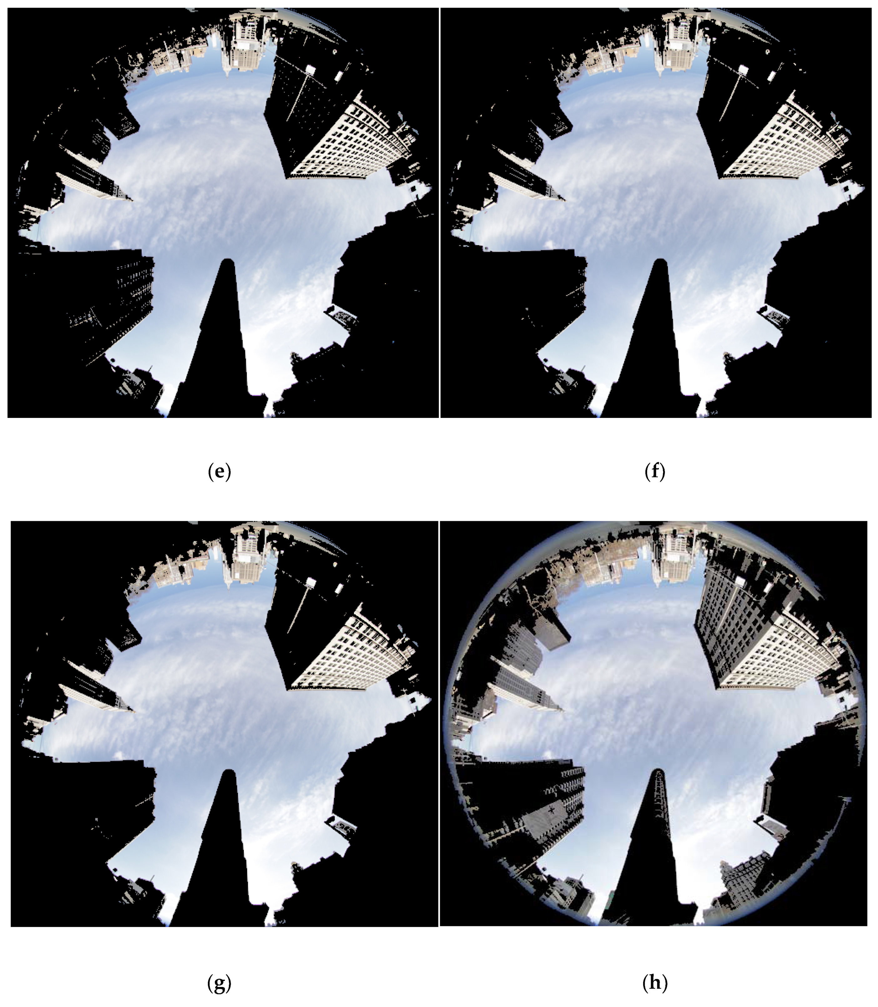
Figure 3.
Block diagram of image processing module and an example of results.

Figure 4.
Comparison of PVT horizontal error given by different discriminators.

Figure 5.
Experimental configuration.
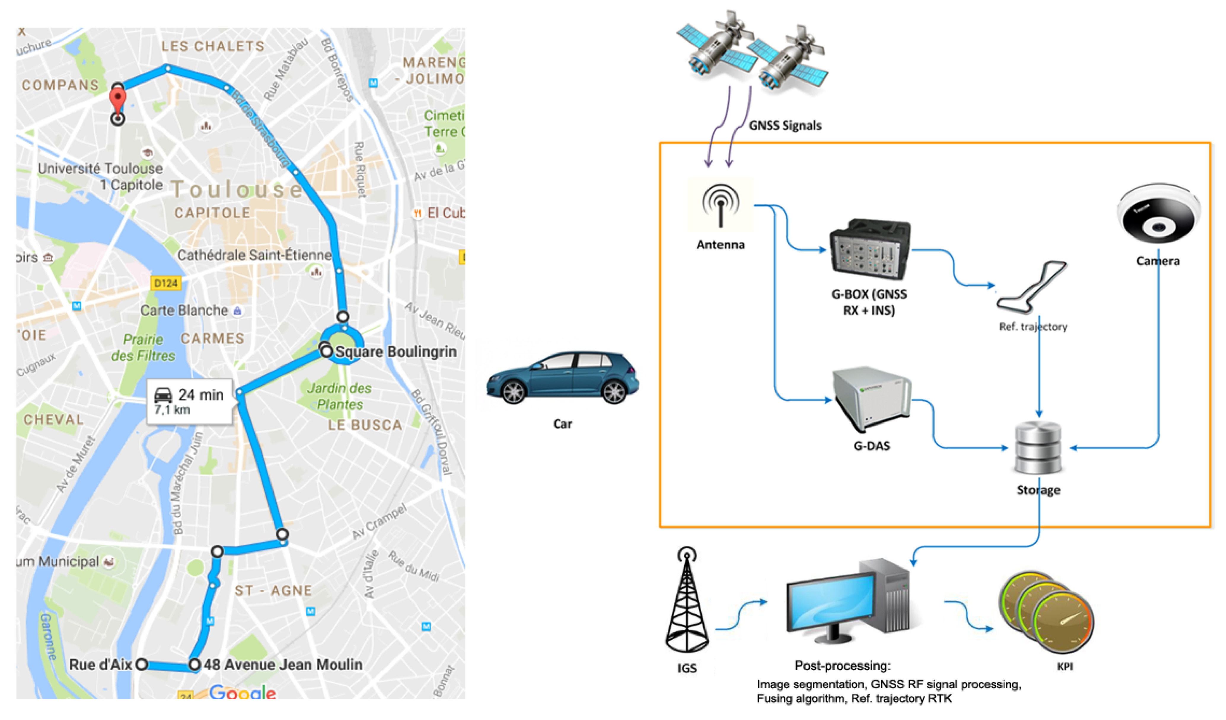
Figure 6.
HPE for the whole track—1800s.

Figure 7.
HPE zoomed around timestamp 850.

Figure 8.
HPL (a) and HDOP (b) around timestamp 850.

Figure 9.
LoS MAP and video at timestamp 861.
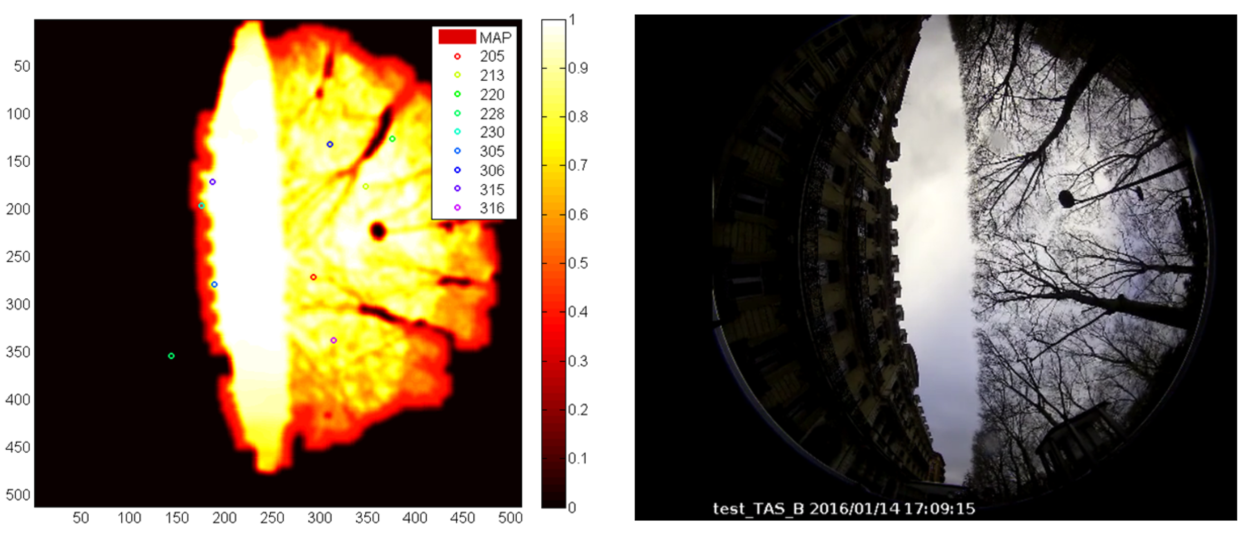
Figure 10.
Pseudorange residuals, C/N0 and LoS probability on SVID GPS 28.

Figure 11.
A pdf of the “clean” (left) and of the “excluded/overweighted” (right) pseudorange residuals for the whole track. The pdfs are represented with red lines and are obtained by fitting the corresponding histograms represented in blue.
Figure 11.
A pdf of the “clean” (left) and of the “excluded/overweighted” (right) pseudorange residuals for the whole track. The pdfs are represented with red lines and are obtained by fitting the corresponding histograms represented in blue.


Table 1.
HPE, HPL and MI with a Kalman filter and proposed camera-based aiding algorithm.
| Camera Module | HPE | HPL | MI | ||||
|---|---|---|---|---|---|---|---|
| 67% | 95% | 99% | 67% | 95% | 99% | ||
| OFF | 4.27 | 8.79 | 12.17 | 31.71 | 41.56 | 58.45 | 0 |
| ON | 3.85 | 6.59 | 10.14 | 36.64 | 47.62 | 78.28 | 0 |
Publisher’s Note: MDPI stays neutral with regard to jurisdictional claims in published maps and institutional affiliations. |
© 2021 by the authors. Licensee MDPI, Basel, Switzerland. This article is an open access article distributed under the terms and conditions of the Creative Commons Attribution (CC BY) license (https://creativecommons.org/licenses/by/4.0/).
Share and Cite
MDPI and ACS Style
David, C.; Nafornita, C.; Gui, V.; Campeanu, A.; Carrie, G.; Monnerat, M. GNSS Localization in Constraint Environment by Image Fusing Techniques. Remote Sens. 2021, 13, 2021. https://0-doi-org.brum.beds.ac.uk/10.3390/rs13102021
AMA Style
David C, Nafornita C, Gui V, Campeanu A, Carrie G, Monnerat M. GNSS Localization in Constraint Environment by Image Fusing Techniques. Remote Sensing. 2021; 13(10):2021. https://0-doi-org.brum.beds.ac.uk/10.3390/rs13102021
Chicago/Turabian StyleDavid, Ciprian, Corina Nafornita, Vasile Gui, Andrei Campeanu, Guillaume Carrie, and Michel Monnerat. 2021. "GNSS Localization in Constraint Environment by Image Fusing Techniques" Remote Sensing 13, no. 10: 2021. https://0-doi-org.brum.beds.ac.uk/10.3390/rs13102021
Note that from the first issue of 2016, this journal uses article numbers instead of page numbers. See further details here.