Article

Species-Level Classification and Mapping of a Mangrove Forest Using Random Forest—Utilisation of AVIRIS-NG and Sentinel Data

by
Mukunda Dev Behera
1,
Surbhi Barnwal
1,
Somnath Paramanik
1,*,
Pulakesh Das
2,
Bimal Kumar Bhattyacharya
3,
Buddolla Jagadish
1,
Parth S. Roy
2,
Sujit Madhab Ghosh
1 and
Soumit Kumar Behera
4
1
Centre for Oceans, Rivers, Atmosphere and Land Sciences (CORAL), Indian Institute of Technology Kharagpur, Kharagpur 721302, India
2
World Resources Institute, New Delhi 110016, India
3
Space Applications Centre, ISRO, Ahmedabad 380015, India
4
Plant Ecology and Climate Change Science Division, CSIR-National Botanical Research Institute, Rana Pratap Marg, Lucknow 226001, India
*
Author to whom correspondence should be addressed.
Remote Sens. 2021, 13(11), 2027; https://0-doi-org.brum.beds.ac.uk/10.3390/rs13112027
Submission received: 13 April 2021 / Revised: 11 May 2021 / Accepted: 13 May 2021 / Published: 21 May 2021

Abstract

:
Although studies on species-level classification and mapping using multisource data and machine learning approaches are plenty, the use of data with ideal placement of central wavelength and bandwidth at appropriate spatial resolution, for the classification of mangrove species is underreported. The species composition of a mangrove forest has been estimated utilising the red-edge spectral bands and chlorophyll absorption information from AVIRIS-NG and Sentinel-2 data. In this study, three dominant species, Heritiera fomes, Excoecaria agallocha and Avicennia officinalis, have been classified using the random forest (RF) model for a mangrove forest in Bhitarkanika Wildlife Sanctuary, India. Various combinations of reflectance/backscatter bands and vegetation indices derived from Sentinel-2, AVIRIS-NG, and Sentinel-1 were used for species-level discrimination and mapping. The RF model showed maximum accuracy using Sentinel-2, followed by the AVIRIS-NG, in discriminating three dominant species and two mixed compositions. This study indicates the potential of Sentinel-2 data for discriminating various mangrove species owing to the appropriate placement of central wavelength and bandwidth in Sentinel-2 at ≥10 m spatial resolution. The variable importance plots proved that species-level classification could be attempted using red edge and chlorophyll absorption information. This study has wider applicability in other mangrove forests around the world.

Graphical Abstract

1. Introduction

Studies on plant species-level classification and mapping using multi-sensor data have always been a challenge, and researchers have attempted to use them for simple mono-formation plantations and tropical mixed forests using various discriminative algorithms. Species-level mapping helps in the better estimation of various biochemical and biophysical parameters, such as pigment concentration, leaf area index, primary productivity, and carbon sequestration, etc., which are useful for forest resource assessment, and for formulating appropriate conservation and management activities. Unlike diverse tropical forests, mangrove species occur in relatively dominant formations, thereby offering some structure to attempt species-level and mixed-groups classification using satellite data. Mapping the spatio-temporal distribution of mangrove forests would help in understanding ongoing changes and project the influence of climate change [1]. The species’ distribution in mangrove forests is primarily regulated by salinity level, distance from the sea or estuary bank, duration and frequency of the tidal inundation, soil composition, etc. [2]. It has been observed that due to the lowering of pH, the concentration of Excoecaria agallocha species is increasing at the expense of Heritiera fomes in the Sunderban mangrove forest, eastern India [3].
The spectral bands and derived indices from the multispectral and hyperspectral remote sensing data are commonly used to distinguish mangrove forest cover from other vegetation. Researchers have classified and mapped mangrove and other species based on their spectral, phenological and physical characteristics, such as height, size, and shape, while several studies have employed chemical characteristics [4,5]. Recently, Grabska et al. [6] mapped nine tree species within mixed forests based on their phenological phase and reported that time-series data use significantly improved forest tree species mapping by approximately 5–10%. Martin et al. [7] classified 11 forest cover types, including pure and mixed stands of deciduous and conifer species. This approach combined species-specific chemical characteristics and previously derived relationships between hyperspectral data and foliar chemistry. However, a few studies have implemented the entire range of spectral values to classify and map mangrove forests. Studies mapping mangrove forest extent using different indices-based approaches were attempted [8,9], with a few on species-level mapping [10,11]. Vegetation spectral indices use two or more spectral bands, and enhance particular properties of different species based on their relative reflectance [12]. The Combined Mangrove Recognition Index (CMRI) is a widely used index for mapping mangrove forest cover [13,14,15]. Ramdani et al. [16] reported a better accuracy in discriminating mangrove species using principal polar spectral (PPS) indices over vegetation indices, such as the Normalized Difference Vegetation Index (NDVI). Moreover, the narrow spectral bands of hyperspectral data are more sensitive to the specific absorption features corresponding to different species [17]. Various studies have demonstrated the utility of various narrow spectral bands in the green, red, red edge, and NIR regions of hyperspectral data in identifying the different mangrove species [18,19,20,21]. In particular, Jusoff et al. [22] explored the potential use of airborne imaging spectrometer for applications (AISA) airborne hyperspectral data to assess nine groups of mangrove species, and observed that they could be easily distinguished in the near-infrared region. Researchers have attempted mangrove species composition mapping using pixel-based classification approaches, such as maximum likelihood classification (MLC), spectral unmixing (SU), and spectral angle mapper (SAM) [23,24,25]. Cho et al. [26] used the SAM classifier to minimise intraspecific spectral variability for discriminating among South African savanna tree species.
Several studies have implemented various microwave datasets for mangrove species classification, as backscatter energy is primarily affected by plant moisture content [2]. Pham et al. [27] classified two mangrove species using a logistics tree model classifier employing the ALOS-2 microwave data. Multi-sensor remotely sensed datasets (e.g., multispectral, hyperspectral, SAR) provide complementary information to improve species-level classification and mapping [28,29]. Cao et al. [30] used object-based classification to identify mangrove species by deriving data synergy from unmanned aerial vehicles (UAVs), hyperspectral images, and digital surface models (DSMs). Zhang et al. [31] integrated optical and microwave data for mangrove species classification using various machine learning models, and obtained good classification accuracy by combining dual polarimetric synthetic aperture radar (SAR) data. Arasumani et al. [32] surveyed classification exercises using a multi-sensor dataset with different machine learning approaches. However, this study implemented random forest (RF), a machine learning model, to discriminate and classify three dominant mangrove plant species. The RF model has the advantage of handling high-dimensional intercorrelated data, and efficiently avoids any overfitting [33]. The RF model also quantifies the level of importance of variables based on the out-of-bag (OOB) data. It indicates the percentage of contribution of each predictor variable used for generating the model [34]. Naidoo et al. [35] integrated hyperspectral and LiDAR measurements using the RF model to improve savanna species identification. Zhang et al. [29] used the Worldview-3 and Radarsat-2 satellite data to classify four mangrove species, and they found that using SAR data, the classification accuracy was not improved remarkably. Wong et al. [28] explored the potential of combining hyperspectral and SAR datasets to map mangrove at the species level, and they suggested using an artificial neural network classifier for achieving more accurate classification. Xia et al. [36] used a multisensor dataset (e.g., Sentinel-1 dual-polarimetric SAR, Sentinel-2 multispectral, and Gaofen-3 full-polarimetric SAR) to cluster the mangrove communities using different pieces of spectral band combination information.
Green pigments exhibit maximum absorption in the red region between 660 and 680 nm. However, the reflectance at these wavelengths is not useful for the prediction of chlorophyll content, as it is relatively saturated with low chlorophyll absorption in the 660–680 nm region, thereby reducing the sensitivity to high chlorophyll contents [37]. The spectral range between the boundary of the red wavelength and the NIR wavelength is called the red edge position, where a sudden rise in the reflectance is observed for healthy vegetation. The red edge has the potential to distinguish healthy vegetation from other land surface features at a site. The red edge is a unique feature of green vegetation because of the higher and lower reflectance in the NIR and red regions, respectively, due to the scattering property of the plant tissue [38]. Researchers have demonstrated the potential use of the red edge wavelength or red edge-based indices to estimate or predict the chlorophyll content of mangrove species or other vegetation types [10,39,40]. The vegetation indices are used as a proxy, statistically linked to field-measured biophysical characteristics and further used for spatio-temporal extrapolation [41]. Suitable vegetation indices employing spectral bands sensitive to chlorophyll pigmentation are widely used in evaluating leaf chlorophyll content, such as the Red Edge Chlorophyll Index (ReCI), Red Edge Normalised Vegetation Index (ReNDVI), and Pigment Specific Normalised Difference for chlorophyll a and b (PSNDa and PSNDb) (Table 1) [42,43,44,45]. The Optimized Soil Adjusted Vegetation Index (OSAVI) exhibited a significant correlation with chlorophyll pigment absorption [46].
The main goal of this study is to test the potential of using narrow bands of AVIRIS-NG and broad bands of Sentinel-1 and 2, and their data synergy, to classify and map three dominant species, using red edge spectral regions as a discriminant of chlorophyll absorption in a mangrove forest in eastern India.

2. Materials and Methods
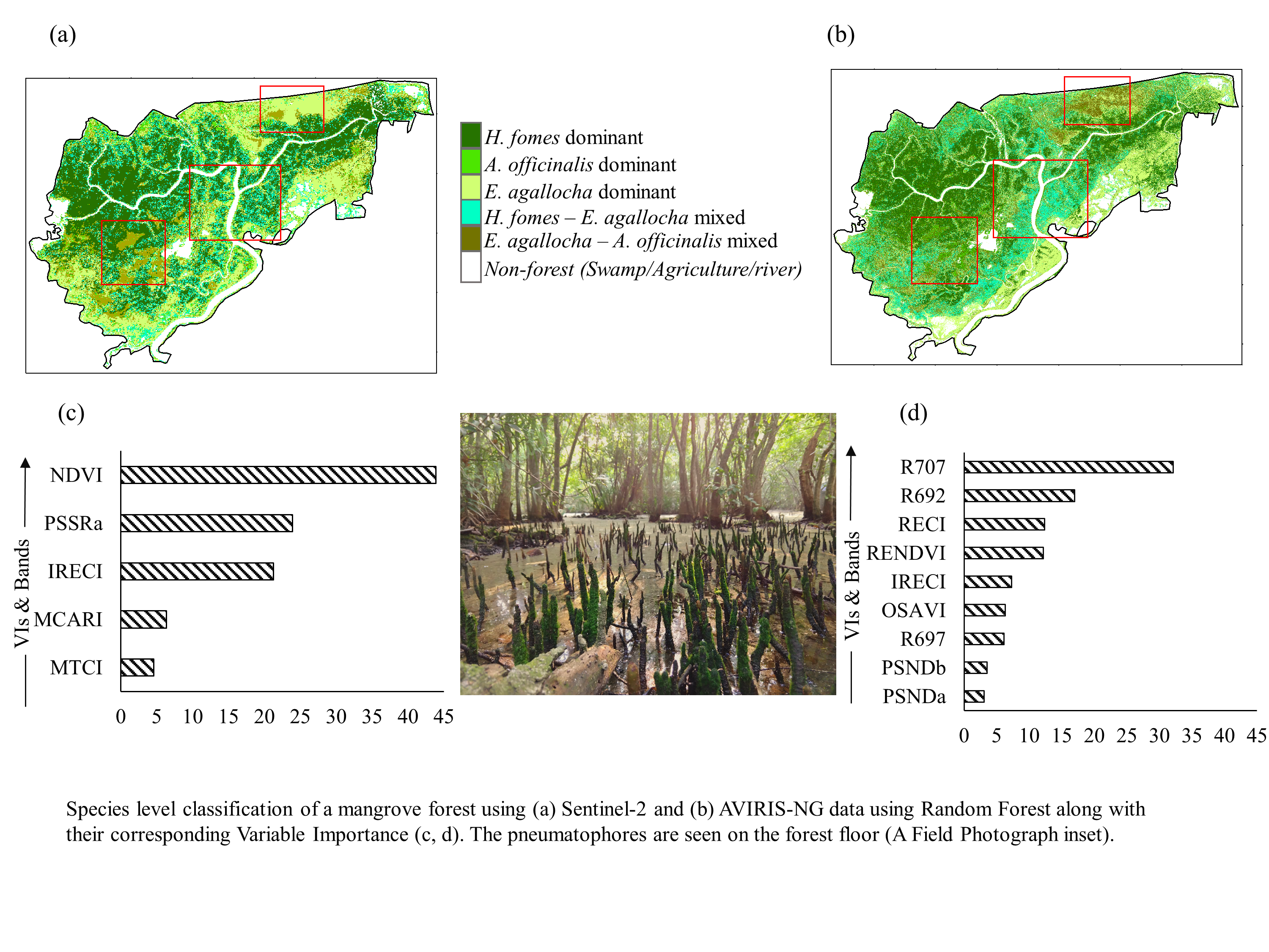
2.1. Study Area

This study was carried out in Bhitarkanika Wildlife Sanctuary (BWS), Odisha, situated on the eastern coast of India between 20°4′N to 20°5′N latitude and 86°49′E to 86°56′E longitude (Figure 1), with an area of about 145 km2. A total of 62 species ofmangrove plants have been recorded in the Dangamal block of BWS, of which 3 species, as Heritiera fomes, Excoecaria agallocha, and Avicennia officinalis, are dominant, followed by Cynometra ramiflora, Sonneratia apetala, Rhizophora mucronata, Aegicera scorniculatum, and Ceriops decandra [54]. BWS is within a tropical warm and humid climate region and receives about 1670 mm of average annual rainfall. The average temperature varies between 10 °C in winter and 43 °C in summer, and the relative humidity ranges from 70% Mean surface reflectance spectra to 84% throughout the year.

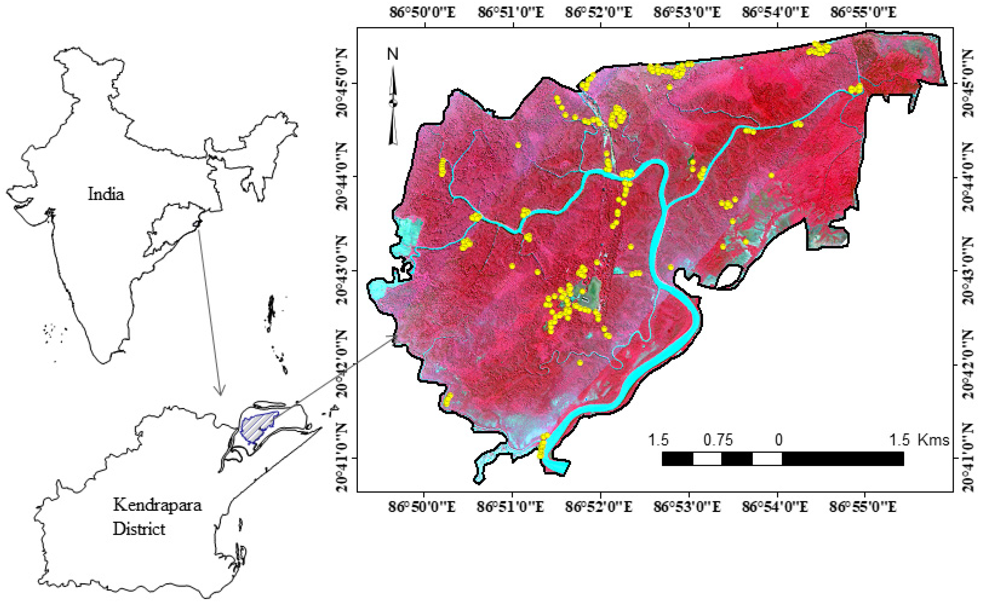
2.2. Satellite and Airborne Data Processing

AVIRIS-NG is a joint airborne campaign carried out by the India Space Research Organisation (ISRO) and National Aeronautics and Space Administration Jet Propulsion Laboratory (NASA JPL) onboard an ISRO B200 aircraft [55]. The onboard hyperspectral sensor recorded DN (Digital Number) values in the spectral range from 380 nm to 2500 nm, with a bandwidth of 5 nm over 425 spectral bands. Flying at a 4 to 8 km altitude, the hyperspectral sensor collected data at 4 to 8 m spatial resolution within a swath of 4 to 6 km. Three levels (L0, L1, and L2) of AVIRIS-NG data are available, where L0 is the raw data captured by the sensor and recorded in the form of DN values, L1 is the ortho-rectified image containing the radiance value (unit µW/sr/nm/cm2), and the L2 data products are the atmospherically corrected surface reflectance data (unitless quantity). For the atmospheric correction, the 6S model and moderate resolution atmospheric transmission (MODTRAN) module were used, which produced the bottom of the atmosphere reflectance data, with the least error ranging from 14.9% to 38.4% with respect to in situ measurements [56]. Four AVIRIS-NG L2 image tiles were used in this classification exercise, of which three were taken on 25 December 2015, and one on 28 December 2015. AVIRIS-NG level-2 data are already pre-processed (geo-rectified, atmospherically corrected), so were directly used for the retrieval of bands and indices after confirming tile rotation and masking out for the BWS site using the ENVI 5.1 platform.
Sentinel-1, launched by the European Space Agency (ESA) in 2014, carries a SAR sensor that operates in the C-band (frequency of 5.4 GHz) and provides dual-polarised images (VV and VH). The dual-polarised images (VV and VH) were downloaded from the Copernicus website (https://scihub.copernicus.eu/dhus/#/home, accessed on: 19 May 2019) for 23 December 2018 and pre-processed to obtain backscattered intensity values, following radiometric calibration, speckle filtering, and terrain correction. Sentinel-2, launched by the ESA in June 2015, uses 13 spectral bands at different spatial resolutions (10, 20, and 60 m). Sentinel-2 data were downloaded and pre-processed using the Sentinel Application Platform (SNAP) software for the date 26 December 2018. The acquisition time of the Sentinel-2 image was 10:12 am (IST). The Sen2cor was used for the atmospheric correction and to generate a bottom-of-atmosphere (BOA) reflectance image that implements different corrections, such as atmosphere, terrain, and cirrus, in the level-1C top-of-atmosphere input data. The pre-processed Sentinel-1 and Sentinel-2 data were resampled to 20 m to match the field sampling mesh size and for utilisation in classification exercises. Tidal information was taken from an open-source software WXTide32, and from the online source (https://tides4fishing.com/as/india/bhitarkanika, accessed on: 29 April 2021). On 26 December 2018, the tidal height had a range between 0.4 m and 2.9 m, whereas for 28th December this range was 0.5 m to 2.7 m. At the time of image acquisition by the Sentinel-2 sensor, the tidal height was about 1.2 m. The two-day image acquisition process covered 26th (at 8:30 am IST) and 28th (at 5:20 am IST) December as part of the AVIRIS-NG campaign; the tidal height was about 0.9 m and 0.7 m on the respective dates.

2.3. Field Data Collection

We laid Elementary Sampling Units (ESUs) of 20 × 20 m2 to record information on the composition on Heritiera fomes, Excoecaria agallocha, and Avicennia officinalis species (Figure S1), including the geolocation (using handheld GPS device) of the centre point of the ESUs. The ESUs were clustered into singlet and duplet species according to the species occurrence within a particular ESU. Throughout our field observation, the tidal height varied between 0.5 m and 2.9 m at high-tide and low-tide, respectively.

2.4. Generation of Vegetation Indices (VIs)

Several vegetation indices were generated that concentrated on the wavelength region of chlorophyll absorption, as well as the red edge region. Six Vis, including ReNDVI, ReCI, IRECI, PSNDa, and PSNDb, and six narrow red edge bands, b64, b65, b66, b67, b68, and b69, were retrieved and pre-processed from the AVIRIS-NG dataset (Table 2). Additionally, OSAVI MCARI, IRECI, NDVI, PSSRa, and MTCI were computed and pre-processed from Sentinel-2 data [39,42,43,44,48,49,50,51].

2.5. Mangrove and Non-Forest Mapping: Spectral Angle Mapper (SAM)

Different species-level classification approaches were adopted employing the bands, VIs, or a combination of hyperspectral (AVIRIS-NG), microwave (Sentinel-1), and/or multispectral (Sentinel-2) sensors. The spectral behaviours of various mangrove species were analysed with respect to their varying wavelengths. Signatures or spectral reflectance curves were generated for the three dominant species, Heritiera fomes, E agallocha and Avicennia officinalis, whereby the mean of nine adjacent pixels was considered. The SAM classification technique was used to distinguish between the mangrove forests and other classes, such as water body, river, grassland, agriculture, and fallow land. The SAM algorithm compares the spectral similarities between the input (reference) spectra and the target spectra, which overcome the solar illumination factor that affects the image’s DN values [57]. The SAM classifier was applied on the AVIRIS-NG and Sentinel-2 imagery, where the ENVI and ArcGIS platforms were used, respectively. The SAM classifier was employed to extract the mangrove forest area. The end members or the pure spectra were collected following the minimum noise fraction (MNF) and pixel purity index (PPI). These end members were used as training sample spectra in the SAM classifier, as it is a supervised classification technique. Several spectra were generated using a field reference corresponding to GPS-based locations. This whole collection of spectral library data for different features, such as wetland, grassland, water bodies, mangroves, and agricultural land, was fed to the classifier as a training set with a 10-degree radian for classification. Here, this classification step was considered an elimination method, as the main goal was to identify different mangroves species and their mixed combinations.

2.6. Species-Level Mapping: Random Forest

The random forest (RF) model is a nonparametric ensemble classification model that uses large numbers of classifiers or trees [58]. Hundreds of trees are used for classification, whereby each tree casts a vote for the output class, and the final output class is determined based on the majority of votes received by all the trees [59]. The RF classifier uses bagging to form an ensemble of classification and induction tree-like classifiers [60]. Two-thirds of the total samples are used as training datasets, and the remaining one-third of the data are used to estimate the out-of-bag (OOB) error [4]. The performance of the RF model depends on two parameters, which are the number of variables, used as the input for the RF model, and the number of decision trees [61]. It can handle high-dimensional and intercorrelated data and efficiently avoid overfitting [8,33]. It quantifies the level of importance of variables based on their OOB data, and indicates the contribution of each predictor variable used for generating the model. VIs and band combinations were used as predictable input variables in the RF model for generating 10 sets of different species-level classifications (Table 2). Out of the total 266 ESUs, 166 ESUs were randomly chosen to develop the classification model, while the remaining 100 ESUs were used to assess the post-classification accuracy. The input data points were split into 70% and 30% for model training and testing, respectively. A 10-fold cross-validation approach was adopted to improve the performance of the model by tuning the “mtry” parameter, whereby the value was optimised based on the least RMSE. With an appropriate model (good overall and Kappa accuracy), the RF model was applied to derive a species-level map of BWS using bands, VIs, and a combination of bands and VIs from different sensors. The “raster”, “rgdal”, “randomForest”, and “caret” packages were used.

2.7. Accuracy Assessment

Accuracy assessment is an important step in the classification process. The goal is to quantitatively determine how effectively pixels were clustered into the correct feature classes according to the ground/reference observations. It is a site-specific method usually assessed by forming a confusion matrix or error matrix, wherein several matrices are used to provide a summary of the classification accuracy including the errors, e.g., omission and commission errors [62,63]. In confusion matrix analysis it is assumed that the pixels are pure, and that the ground samples/reference points are perfectly co-located on the classified image where the proportion of mixed pixels depends upon the spatial resolution of the imagery [64]. Finally, a coefficient of agreement between classified image and reference points data was calculated using the Kappa coefficient, which indicates the actual agreement between the classification and the observation. The value of the Kappa coefficient lies between 0 and 1, where the higher values represent a better agreement between the two datasets. The Kappa coefficient is calculated using the following equation [65]:
K = (P0 − Pe)/(1 − Pe)
where Po is the proportion of cases correctly classified and Pe is the expected proportion of cases correctly classified by chance.
All of the data processing steps are depicted in the methodology flowchart (Figure 2).

3. Results

3.1. Field Assessment of Species Distribution

The dominance of Heritiera fomes, Excoecaria agallocha, and Avicennia officinalis species at various proportions were observed at the Bhitakanika Wildlife Sanctuary. The next most dominant mangrove species were Cynometra ramiflora and Bruguiera gymnorhiza. Plots were laid to record the data for pure and mixed formations in various spatial distribution locations. In total, 30, 19 and 10 ESUs were dominated by Heritiera fomes at >90%, 80 to 89% and >70 to 79%, respectively (Table 3). A total of 57 and 36 ESUs were laid in patches dominated at >90% and 80 to 89% by the three candidate species. Further, a total of 27, 22, and 24 ESUs showed duplet combinations of Heritiera fomesExcoecaria agallocha and Excoecaria agallochaAvicennia officinalis at >70 to 79%, >60 to 69%, and >50 to 59%, respectively (Table 3). It was also observed that Avicennia officinalis has the highest canopy cover among the three dominant species, which is why the number of trees per ESU is lower, even though they are sparser.

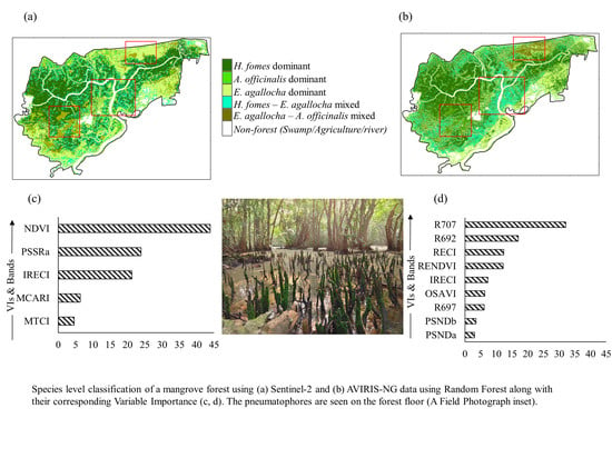
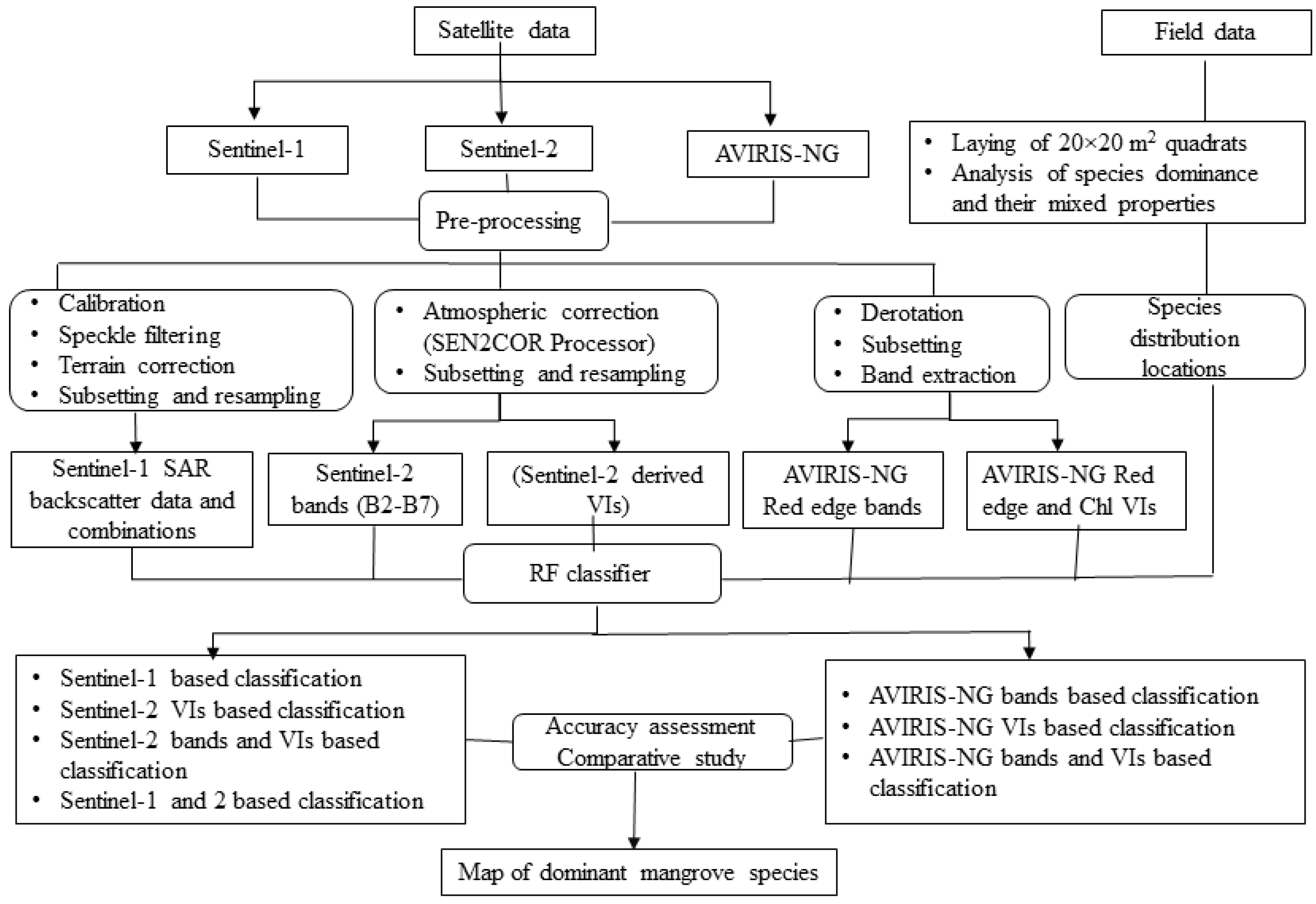
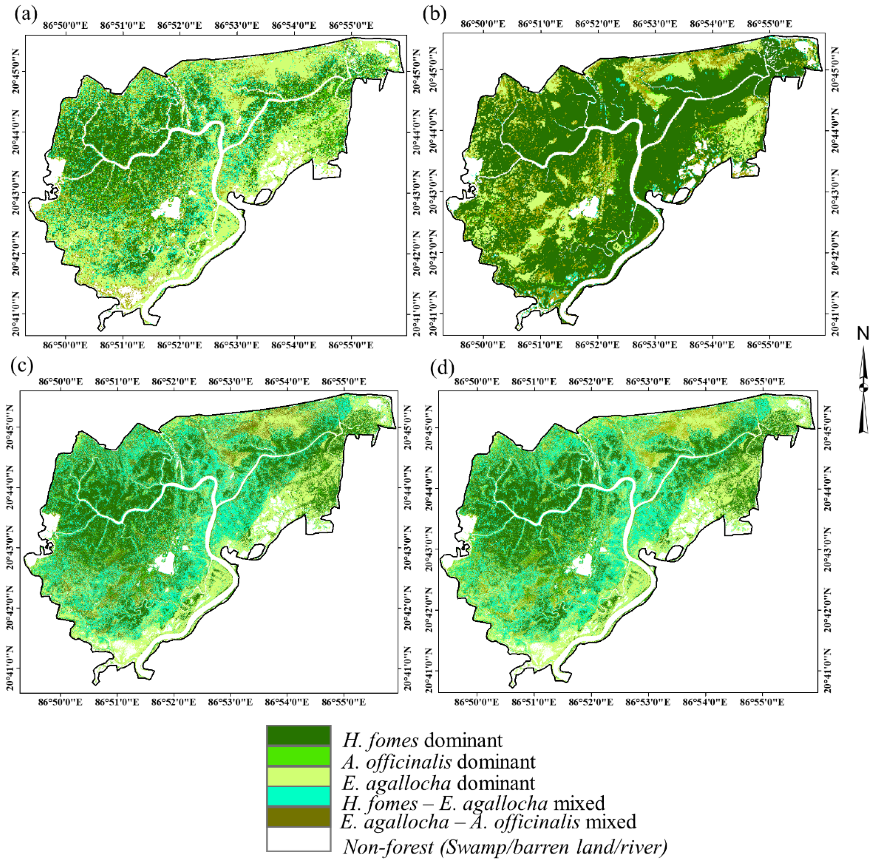
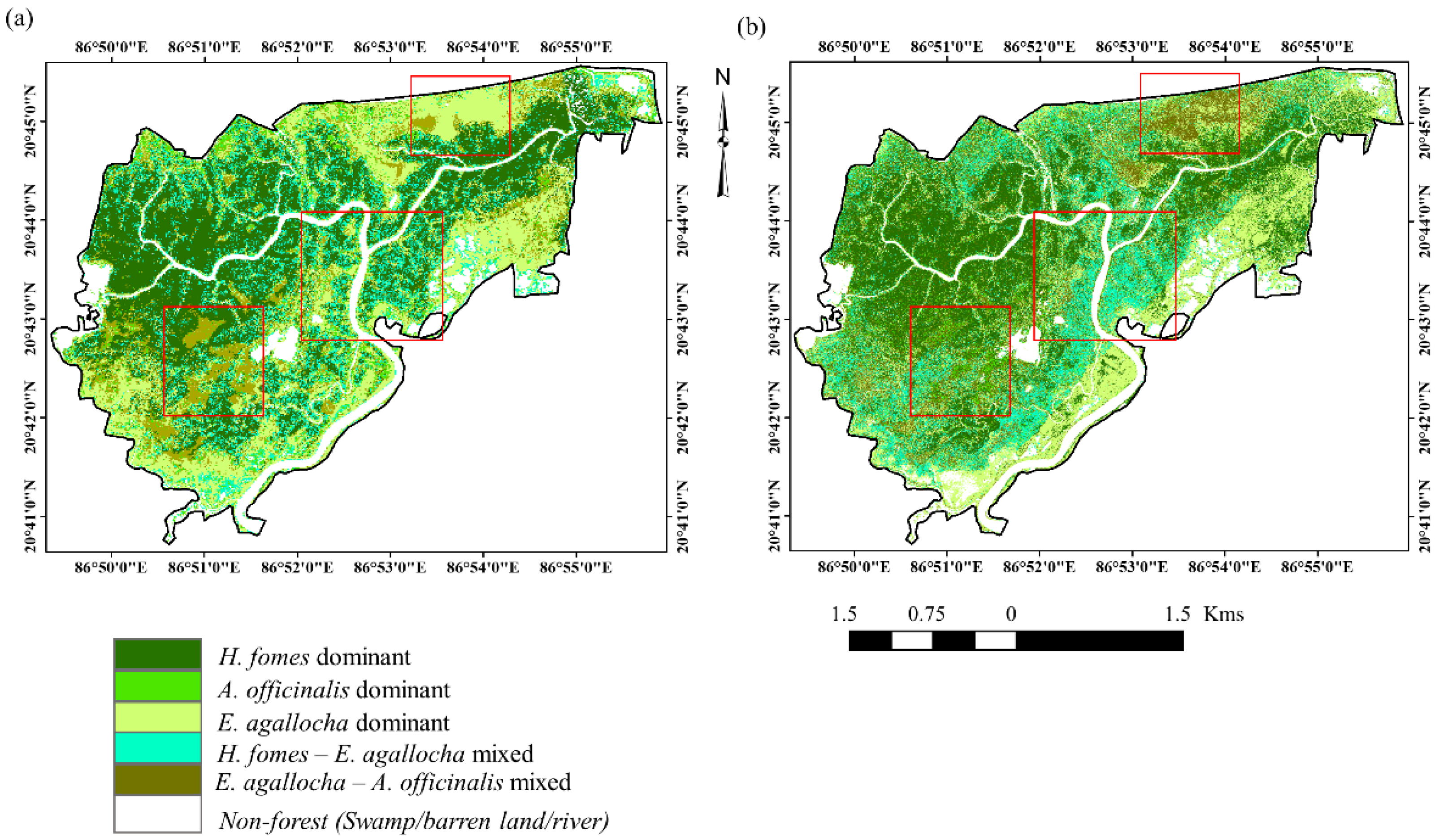
3.2. Species-Level Classification and Mapping Using RF Model

The spectral analysis indicates minor differences in chlorophyll absorption and red edge wavelength ranges for the three dominant species. However, the reflectance intensity indicates significant differences in the NIR and SWIR regions, where Avicennia officinalis has a higher reflectance than the other two species, indicating similar spectral reflectance (Figure S2). The SAM classifier helped in discriminating vegetation and non-vegetation areas in BWS. However, species-level classification using the SAM supervised classifier did not perform well in this study. The SAM classification output provided a broad classified map, where the mangrove region was segregated from other features in order to mark out other areas from the entire image before classification with the RF model.
Using six narrow AVIRIS-NG hyperspectral bands (in the red edge spectral range), the RF model demonstrated 55% overall accuracy, which further improved to over 70% using six VIs and three narrow bands; however, the kappa accuracy was low (Table 2). The RF model improved the overall and Kappa accuracy of various Sentinel-2 data-derived VIs (five vegetation indices, MCARI, IRECI, NDVI, PSSRa, MTCI), with the maxima of 74% overall and 0.61 Kappa accuracy (Table 2). Sentinel-1 dual-pol SAR data with VH, VV, VH ×VV, and ((VV + VV)/2) combinations demonstrated only 48% overall and 0.33 Kappa accuracy. However, the combination of Sentinel-1 and 2 bands and VIs demonstrated good overall (67.5%) and Kappa (0.54) accuracy (Table 2).
It was found that the Heritiera fomes are dominantly distributed in the highlands of BWS, mostly in homogenous and contiguous patches (Figure 3a–d). The patches of Heritiera fomes are dominant in the eastern and western parts of BWS along the creeks. Compared to other species, the distribution of Heritiera fomes is more similar, as derived using the AVIRIS-NG and Sentinel-2 data (Figure 4a,b). The southern and peripheral regions of the sanctuary are dominated with Avicennia officinalis and Excoecaria agallocha species in different proportions. The dominant compositions of Heritiera fomes, Excoecaria agallocha and Avicennia officinalis cover 17.29 km2, 12.37 km2, and 3.13 km2, respectively. Mixed species such as Heritiera fomesExcoecaria agallocha and Excoecaria agallochaAvicennia officinalis are found distributed over 7.6 km2 and 5.5 km2, respectively. The swamp, agricultural land, river, waterbody, and fallow land cover 5.9 km2. These area statistics were calculated using the map derived from the Sentinel-2 dataset.
The post-classification accuracy was assessed using 100 data points, revealing a maximum overall accuracy of 69% and Kappa accuracy of 0.59 using AVIRIS-NG narrow bands and vegetation indices, followed by 50% (0.34) and 38% (0.2) for Sentinel-2 VIs and Sentinel 1 and 2 combinations, respectively. The user’s and producer’s accuracy for the pure classes is estimated to be higher for Heritiera fomes than Avicennia officinalis and Excoecaria agallocha, whereas for mixed classes, the accuracy was observed to be higher for Heritiera fomes and Avicennia officinalis compared to Avicennia officinalis and Excoecaria agallocha.

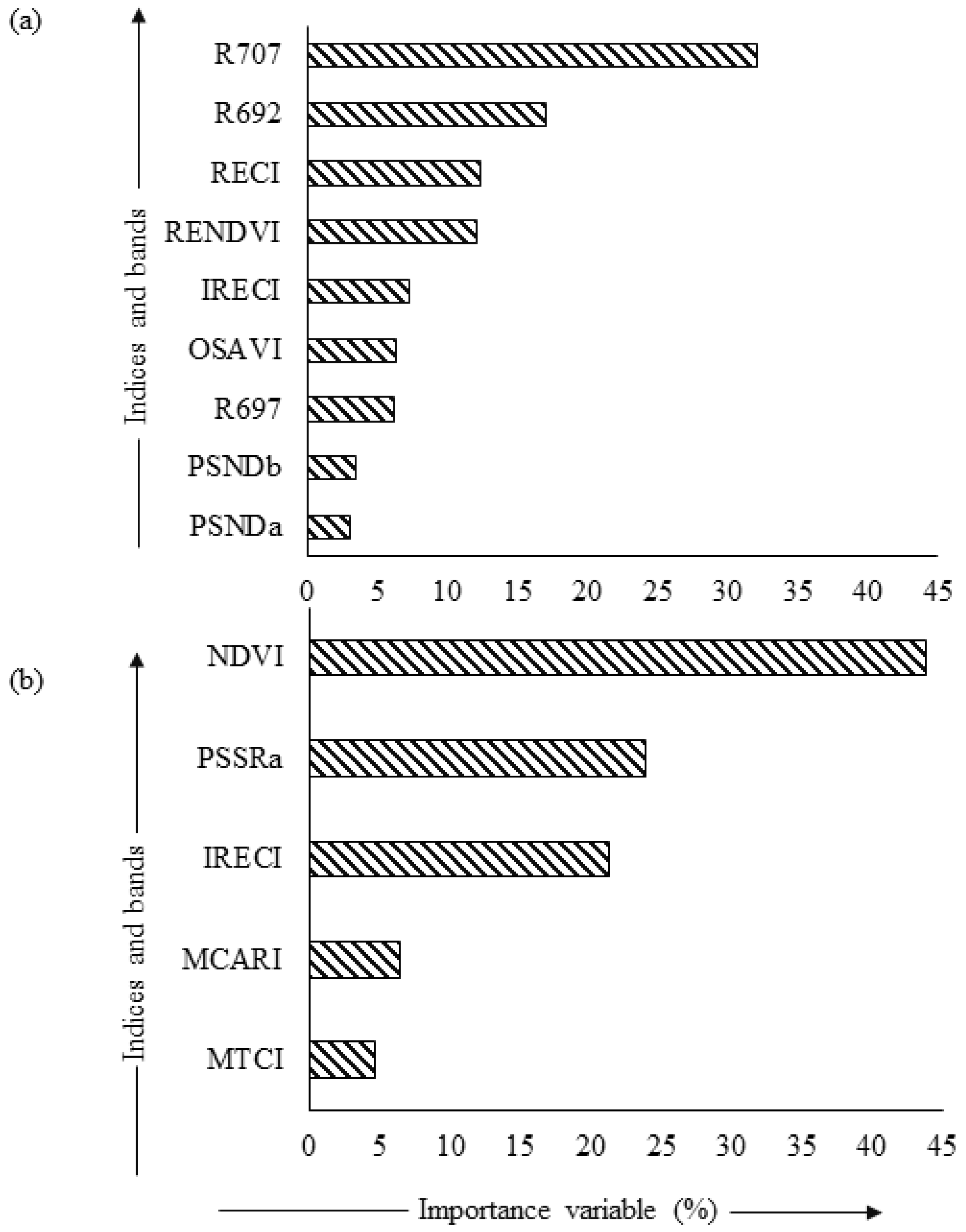
3.3. Importance Variables

The importance ranking retrieved using AVIRIS-NG data revealed that the red edge band (B077) exhibited the maximum contribution (32%), followed by B692 (17%), RECI, and RENDVI, which contributed equally (12%) to species-level classification (Figure 5a). The importance plots derived using Sentinel-2-based VIs revealed that red edge-based indices such as NDVI (44%), PSSRa (24%), and IRECI (21%) make the maximum contributions in the RF model-based species-level classification (Figure 5b). This plot highlights the most important variables and their contributions to the classification results derived with the RF model.

4. Discussion

Species occurrences were recorded on the ground according to the stand density in the ESU scale with geolocation information. It may be noted that the Sentinel 1 and 2 pixels nearly matched with the dimension (20 × 20 m2) of the ESU, while the 25 (5 × 5 m2) AVIRIS-NG pixels corresponded to one ESU. It should be mentioned that extensive fieldwork in this ecosystem is challenging due to the presence of pneumatophores, networks of creeks, and mud owing to the tidal effects. According to field observations, the impact of the tidal effect on this study is minimal, as the maximum tidal height was almost 1.2 m on the image acquisition date. It was found that the Heritiera fomes are dominantly distributed in the highlands of BWS, and their distribution is mostly homogenous. Avicennia officinalis and Excoecaria agallocha species are dominant in the peripheral regions of the sanctuary at different proportions. The spatial distributions of different species could indicate the effects of tidal inundation and the species-specific salt tolerance capacity. As species-wise ground spectra were unavailable, the spectral signature collected from the image highlighted the differential spectral responses of the three dominant species Heritiera fomes, Excoecaria agallocha, and Avicennia officinalis [66]. The spectral analysis of Avicennia officinalis showed higher reflectance in the NIR region; this may have been caused by the structure of the leaves and the leaf phenology phase. Comparatively, the leaves of Avicennia officinalis are spongier or softer than those of the other two selected species because of the spongy mesophyll cells, which induce higher reflectance in the NIR region.
The broad band Sentinel-2 data revealed the maximum classification accuracy (74%) followed by narrow hyperspectral AVIRIS-NG data (70.2%) in discriminating three dominant species and two mixed compositions (Table 2; Figure 4a,b). Green et al. [67] reported that high-resolution data may not always yield better results in mangrove species mapping due to the presence of mixed pixels, a background soil–water effect, and spectral saturation in the higher biomass range. However, the ground-based spectral observation provides better results for mapping mangrove species [68], which are often poorly interpreted from satellite imagery [11]. This study used 166 ground-based ESU observations for developing the RF model, wherein both the pure and mixed-species compositions were used for model training to minimise model bias [69]. Our training samples were selected from both homogeneous and heterogeneous ESUs to maintain unbiasedness and a higher classification accuracy, as stated by Millard and Richardson [69]. Kumar et al. [18] focussed on the classification of duplet combinations of mangrove species in BWS, while this study classified and mapped three dominant species (Heritiera fomes, Excoecaria agallocha and Avicennia officinalis) and two duplets (Heritiera fomes, Excoecaria agallocha and Excoecaria agallocha and Avicennia officinalis). Pandey et al. [20] mapped Cerbera oddolam as a dominant mangrove species out of the ten species identified in their study in BWS. Heenkenda et al. [10] employed the much higher resolution Worldview-2 imagery and identified five mangrove species using the support vector machine (SVM) model. Zhu et al. [70] used the Worldview-2 dataset and observed 87% classification accuracy, thereby affording them better results given the higher resolution of the data used. Though spatial information is vital in accurate classification, here, the 4 m AVIRIS-NG provided marginally inferior accuracy compared to the 20 m Sentinel-2 data. The higher performance of Sentinel-2 broad bands indicates the ideal placement of the central wavelengths of important absorption bands [71].
Xia et al. [36] attempted the classification of mangrove species using multisource remotely sensed data and found that SAR provided poor results for classifying mixed stands, which was also observed here. Even data synergy with the addition of SAR (Sentinel-1) with multispectral (Sentinel-2) data did not improve the result (Table 2). The Sentinel-1 SAR has a shorter wavelength (C-band) that receives similar backscattering signals from all the species and thus enables discrimination among them [72]. However, a study conducted by Zhang et al. [29] on a mangrove ecosystem in Hong Kong observed that the ensemble of optical and microwave datasets yielded better results in classifying different plant species than with an individual dataset.
Our study attempted to map mangrove species based on NIR and red edge-based vegetation indices without in situ spectral measurements (Figure 3 and Figure 4). Zhang et al. [73] performed an in situ spectral analysis to separate the mangrove species based on spectral features, and they mentioned that chlorophyll absorption and red edge position are highly important, as confirmed in this study in BWS, eastern India. The importance variable plots derived for AVIRIS-NG and Sentinel-2 data also revealed that species-level classification can be better attempted using red edge bands, red edge-based indices, and chlorophyll absorption-based indices, as they differ the most in these two regions [74,75]. In general, the red edge band is used for plant health assessment, but this study found that the red edge region holds the key for species-level discrimination and mapping of mangrove forests.
Species-level discrimination was possible using the RF model as it uses a subset of features to build individual clusters, based on a decision made via effective features that reduces the error for the entire feature vector. The RF model evaluated each attribute internally [76], and handled the predictor variables well, thus giving multimodal distribution, and the parameter tuning was easy (Table 2). Arasumani et al. [32] recommended the use of an RF model for species-level mapping via Sentinel-2 data in the absence of any hyperspectral imagery.
Our study has proven that the Sentinel-2 dataset has comparatively better potential to perform species-level classification. This could be attributed to the ideal placement of the central wavelength and the appropriate bandwidth. Hyperspectral data have a finer resolution, giving a salt and pepper effect on the classified map, which is not observed in the Sentinel-2 data-derived map. The majority of the species’ occurrences are well-mapped for both the AVIRIS-NG and Sentinel-2 data-derived maps. Few regions indicated dissimilarities; such regions suggest higher uncertainty in species mapping (red boxes, Figure 4a,b), mainly concerning the Excoecaria agallocha and Excoecaria agallocha–Avicennia officinalis mixed classes, whereas Heritiera fomes followed almost the same distribution in both the maps. The higher uncertainty in certain regions may be due to the background soil reflectance caused by lower canopy cover, which could be the reason for the greater uncertainty in the Avicennia officinalis-dominated area.

5. Conclusions

Delineating the species distribution of mangrove forests using remotely sensed datasets is useful for understanding their ecological behaviour. Of all bands and VIs used, both AVIRIS-NG and Sentinel-2 provided comparable results, with the latter showing marginally better accuracy. This study focused on the potential of red edge bands and chlorophyll absorption bands for species-level mapping of a mangrove forest. The results indicated that red edge bands and their corresponding indices are useful for species discrimination. Further attempt at species-level mapping could be made by incorporating the reflectance bands within 900 nm to 1300 nm and 1533 nm to 1954 nm regions using AVIRIS-NG narrow bands. In previous studies, researchers achieved higher accuracy by merging multi-sensor datasets, but our study revealed that a single-sensor dataset (especially Sentinel-2 and AVIRIS-NG) also has the potential to improve accuracy in classification. This study also exemplifies that the combination of multisensor (Sentinel-1 and 2) data may not always perform well, especially in mangrove forests, as Sentinel-1 is not capable of generating species-wise clusters. However, the higher performance of Sentinel-2 broad bands reiterates the importance of the placement of the central wavelengths in absorption bands. This study exemplifies the potential of broad Sentinel-2 and narrow AVIRIS-NG bands to classify and map three dominant species, using the red edge spectral region as the discriminant, in a mangrove forest in eastern India. Further, advanced machine learning models, such as RF, handled the predictor variables well, enabling multimodal distribution for optimal classification.

Supplementary Materials

The following are available online at https://0-www-mdpi-com.brum.beds.ac.uk/article/10.3390/rs13112027/s1, Figure S1: Field photographs of (a) Heritiera fomes, (b) Excoecaria agallocha, and (c) Avicennia officinalis stands measured during field visit, Figure S2: Mean surface reflectance spectra (VNIR wavelength region) generated using nine adjacent pixels dominated with Heritiera fomes, E agallocha and Avicennia officinalis.

Author Contributions

Conceptualisation, M.D.B., S.P., and S.B.; methodology, M.D.B., S.B., S.P., and B.J.; software, S.B., B.J. and S.P.; validation, S.M.G., S.P., S.B. and B.J.; formal analysis, M.D.B., S.B., S.P., P.D. and B.J.; investigation, M.D.B., S.P., P.S.R. and S.K.B.; resources, M.D.B., B.K.B., P.S.R. and S.K.B.; data curation, S.B. and B.J.; writing—original draft preparation, S.B., S.P. and M.D.B.; writing—review and editing, P.D., P.S.R., B.K.B. and S.K.B.; visualisation, M.D.B., S.B. and S.P.; supervision, M.D.B., B.K.B. and P.S.R.; project administration, B.K.B. and M.D.B.; funding acquisition, M.D.B. All authors have read and agreed to the published version of the manuscript.

Funding

This research was funded by Space Applications Centre, ISRO, Ahmedabad, India. P.S.R. is one of the authors who takes care of the APC.

Institutional Review Board Statement

Not Applicable.

Informed Consent Statement

Not Applicable.

Data Availability Statement

Not applicable.

Acknowledgments

M.D.B. is thankful to SAC-ISRO, Ahmedabad for financial support in form of a research funding for AVIRIS-NG AO project. S.P., and B.J. is thankful to IIT Kharagpur for MHRD fellowship to pursue Ph.D. research. All Authors are thankful to the authorities of CORAL and IIT Kharagpur for providing laboratory facilities. The authors are also thankful to Odisha state forest and wildlife department for permission for field visit. The support extended by Nirakar Behera during field work is thankfully acknowledged and greatly appreciated.

Conflicts of Interest

The authors declare no conflict of interest. The funders had no role in the design of the study; in the collection, analysis, or interpretation of data; in the writing of the manuscript, or in the decision to publish the results.

References

  1. Behera, M.D.; Roy, P.S. Forest Remote Sensing, Biodiversity and Climate Change. Curr. Sci. 2012, 102, 1083–1084. [Google Scholar]
  2. Kuenzer, C.; Bluemel, A.; Gebhardt, S.; Quoc, T.V.; Dech, S. Remote Sensing of Mangrove Ecosystems: A Review. Remote Sens. 2011, 3, 878–928. [Google Scholar] [CrossRef] [Green Version]
  3. Behera, M.D. Sundari (H. Fomes)—An Indicator Species of Sundarbans. In Compendium of Biodiversity in Ganga River System; Tare, V., Mathur, R.P., Eds.; LAP Lambert Academic Publishing: Sunnyvale, CA, USA, 2019; pp. 261–278. ISBN 978-613-9-92340-3. [Google Scholar]
  4. Mickelson, J.G.; Civco, D.L.; Silander, J.A. Delineating Forest Canopy Species in the Northeastern United States Using Multi-Temporal TM Imagery. Photogramm. Eng. Remote Sens. 1998, 64, 891–904. [Google Scholar]
  5. Hill, R.A.; Wilson, A.K.; George, M.; Hinsley, S.A. Mapping Tree Species in Temperate Deciduous Woodland Using Time-Series Multi-Spectral Data. Appl. Veg. Sci. 2010, 13, 86–99. [Google Scholar] [CrossRef]
  6. Grabska, E.; Hostert, P.; Pflugmacher, D.; Ostapowicz, K. Forest Stand Species Mapping Using the Sentinel-2 Time Series. Remote Sens. 2019, 11, 1197. [Google Scholar] [CrossRef] [Green Version]
  7. Martin, M.E.; Newman, S.D.; Aber, J.D.; Congalton, R.G. Determining Forest Species Composition Using High Spectral Resolution Remote Sensing Data. Remote Sens. Environ. 1998, 65, 249–254. [Google Scholar] [CrossRef]
  8. Wang, T.; Zhang, H.; Lin, H.; Fang, C. Textural-Spectral Feature-Based Species Classification of Mangroves in Mai Po Nature Reserve from Worldview-3 Imagery. Remote Sens. 2016, 8, 24. [Google Scholar] [CrossRef] [Green Version]
  9. Baloloy, A.B.; Blanco, A.C.; Raymund Rhommel, R.R.C.; Nadaoka, K. Development and Application of a New Mangrove Vegetation Index (MVI) for Rapid and Accurate Mangrove Mapping. ISPRS J. Photogramm. Remote Sens. 2020, 166, 95–117. [Google Scholar] [CrossRef]
  10. Heenkenda, M.K.; Joyce, K.E.; Maier, S.W.; Bartolo, R. Mangrove Species Identification: Comparing WorldView-2 with Aerial Photographs. Remote Sens. 2014, 6, 6064–6088. [Google Scholar] [CrossRef] [Green Version]
  11. Heumann, B.W. An Object-Based Classification of Mangroves Using a Hybrid Decision Tree-Support Vector Machine Approach. Remote Sens. 2011, 3, 2440–2460. [Google Scholar] [CrossRef] [Green Version]
  12. Behera, M.D.; Kushwaha, S.P.S.; Roy, P.S. Forest Vegetation Characterization and Mapping Using IRS-1C Satellite Images in Eastern Himalayan Region. Geocarto Int. 2001, 16, 53–62. [Google Scholar] [CrossRef]
  13. Sudhakar Reddy, C.; Pattanaik, C.; Murthy, M.S.R. Current Science Association Assessment and Monitoring of Mangroves of Bhitarkanika Wildlife Sanctuary, Orissa, India Using Remote Sensing and GIS Author(s): C. Sudhakar Reddy, Chiranjibi Pattanaik and M.S.R. Murthy Published by: Current Scien. Current Sci. Assoc. 2018, 92, 1409–1415. [Google Scholar]
  14. Kumar, A.; Stupp, P.; Dahal, S.; Remillard, C.; Bledsoe, R.; Stone, A.; Cameron, C.; Rastogi, G.; Samal, R.; Mishra, D.R. A Multi-Sensor Approach for Assessing Mangrove Biophysical Characteristics in Coastal Odisha, India. Proc. Natl. Acad. Sci. India Sect. A Phys. Sci. 2017, 87, 679–700. [Google Scholar] [CrossRef]
  15. Gupta, K.; Mukhopadhyay, A.; Giri, S.; Chanda, A.; Datta Majumdar, S.; Samanta, S.; Mitra, D.; Samal, R.N.; Pattnaik, A.K.; Hazra, S. An Index for Discrimination of Mangroves from Non-Mangroves Using LANDSAT 8 OLI Imagery. MethodsX 2018, 5, 1129–1139. [Google Scholar] [CrossRef]
  16. Ramdani, F.; Rahman, S.; Giri, C. Principal Polar Spectral Indices for Mapping Mangroves Forest in South East Asia: Study Case Indonesia. Int. J. Digit. Earth 2019, 12, 1103–1117. [Google Scholar] [CrossRef]
  17. Kishore, M.; Kulkarni, S.B. Hyperspectral Imaging Technique for Plant Leaf Identification. In Proceedings of the 2015 International Conference on Emerging Research in Electronics, Computer Science and Technology, ICERECT 2015, Mandya, India, 17–19 December 2015; pp. 209–213. [Google Scholar] [CrossRef]
  18. Kumar, T.; Panigrahy, S.; Kumar, P.; Parihar, J.S. Classification of Floristic Composition of Mangrove Forests Using Hyperspectral Data: Case Study of Bhitarkanika National Park, India. J. Coast. Conserv. 2013, 17, 121–132. [Google Scholar] [CrossRef]
  19. Padma, S.; Sanjeevi, S. Jeffries Matusita-Spectral Angle Mapper (JM-SAM) Spectral Matching for Species Level Mapping at Bhitarkanika, Muthupet and Pichavaram Mangroves. Int. Arch. Photogramm. Remote Sens. Spat. Inf. Sci. ISPRS Arch. 2014, 40, 1403–1411. [Google Scholar] [CrossRef] [Green Version]
  20. Pandey, P.C.; Anand, A.; Srivastava, P.K. Spatial Distribution of Mangrove Forest Species and Biomass Assessment Using Field Inventory and Earth Observation Hyperspectral Data. Biodivers. Conserv. 2019, 28, 2143–2162. [Google Scholar] [CrossRef]
  21. Chaube, N.R.; Lele, N.; Misra, A.; Murthy, T.V.R.; Manna, S.; Hazra, S.; Panda, M.; Samal, R.N. Mangrove Species Discrimination and Health Assessment Using AVIRIS-NG Hyperspectral Data. Curr. Sci. 2019, 116, 1136–1142. [Google Scholar] [CrossRef]
  22. Jusoff, K. Individual Mangrove Species Identification and Mapping in Port Klang Using Airborne Hyperspectral Imaging. J. Sustain. Sci. Manag. 2006, 1, 27–36. [Google Scholar]
  23. Demuro, M.; Chisholm, L. Assessment of Hyperion for Characterizing Mangrove Communities. In Proceedings of the 12th JPL AVIRIS airborne earth science workshop, Pasadena, CA, USA, 12 February 2003; Volume 31, pp. 18–23. [Google Scholar]
  24. Yang, C.; Everitt, J.H.; Fletcher, R.S.; Jensen, R.R.; Mausel, P.W. Mapping Black Mangrove along the South Texas Gulf Coast Using AISA+ Hyperspectral Imagery. In Proceedings of the Indiana State University—21st Biennial Workshop on Aerial Photography, Videography and High Resolution Digital Imagery for Resource Assessment 2007, Terre Haute, Indiana, 15–17 May 2007; Volume 75, pp. 143–153. [Google Scholar]
  25. Thomas, N.; Lucas, R.; Bunting, P.; Hardy, A.; Rosenqvist, A.; Simard, M. Distribution and Drivers of Global Mangrove Forest Change, 1996–2010. PLoS ONE 2017, 12, e0179302. [Google Scholar] [CrossRef] [Green Version]
  26. Cho, M.A.; Debba, P.; Mathieu, R.; Naidoo, L.; Van Aardt, J.; Asner, G.P. Improving Discrimination of Savanna Tree Species through a Multiple-Endmember Spectral Angle Mapper Approach: Canopy-Level Analysis. IEEE Trans. Geosci. Remote Sens. 2010, 48, 4133–4142. [Google Scholar] [CrossRef]
  27. Pham, T.D.; Bui, D.T.; Yoshino, K.; Le, N.N. Optimized Rule-Based Logistic Model Tree Algorithm for Mapping Mangrove Species Using ALOS PALSAR Imagery and GIS in the Tropical Region. Environ. Earth Sci. 2018, 77, 1–13. [Google Scholar] [CrossRef]
  28. Wong, F.K.K.; Fung, T. Combining EO-1 Hyperion and Envisat ASAR Data for Mangrove Species Classification in Mai Po Ramsar Site, Hong Kong. Int. J. Remote Sens. 2014, 35, 7828–7856. [Google Scholar] [CrossRef]
  29. Zhang, H.; Wang, T.; Liu, M.; Jia, M.; Lin, H.; Chu, L.M.; Devlin, A.T. Potential of Combining Optical and Dual Polarimetric SAR Data for Improving Mangrove Species Discrimination Using Rotation Forest. Remote Sens. 2018, 10, 467. [Google Scholar] [CrossRef] [Green Version]
  30. Cao, J.; Leng, W.; Liu, K.; Liu, L.; He, Z.; Zhu, Y. Object-Based Mangrove Species Classification Using Unmanned Aerial Vehicle Hyperspectral Images and Digital Surface Models. Remote Sens. 2018, 10, 89. [Google Scholar] [CrossRef] [Green Version]
  31. Zhang, H.; Xu, R. Exploring the Optimal Integration Levels between SAR and Optical Data for Better Urban Land Cover Mapping in the Pearl River Delta. Int. J. Appl. Earth Obs. Geoinf. 2018, 64, 87–95. [Google Scholar] [CrossRef]
  32. Arasumani, M.; Singh, A.; Bunyan, M.; Robin, V. Testing the Efficacy of Hyperspectral (AVIRIS-NG), Multispectral (Sentinel-2) and Radar (Sentinel-1) Remote Sensing Images to Detect Native and Invasive Non-Native Trees. Biol. Invasions 2021, 1–17. [Google Scholar] [CrossRef]
  33. Belgiu, M.; Drăgu, L. Random Forest in Remote Sensing: A Review of Applications and Future Directions. ISPRS J. Photogramm. Remote Sens. 2016, 114, 24–31. [Google Scholar] [CrossRef]
  34. Wang, D.; Wan, B.; Qiu, P.; Su, Y.; Guo, Q.; Wang, R.; Sun, F.; Wu, X. Evaluating the Performance of Sentinel-2, Landsat 8 and Pléiades-1 in Mapping Mangrove Extent and Species. Remote Sens. 2018, 10, 1468. [Google Scholar] [CrossRef] [Green Version]
  35. Naidoo, L.; Cho, M.A.; Mathieu, R.; Asner, G. Classification of Savanna Tree Species, in the Greater Kruger National Park Region, by Integrating Hyperspectral and LiDAR Data in a Random Forest Data Mining Environment. ISPRS J. Photogramm. Remote Sens. 2012, 69, 167–179. [Google Scholar] [CrossRef]
  36. Xia, J.; Yokoya, N.; Pham, T.D. Probabilistic Mangrove Species Mapping with Multiple-Source Remote-Sensing Datasets Using Label Distribution Learning in Xuan Thuy National Park, Vietnam. Remote Sens. 2020, 12, 3834. [Google Scholar] [CrossRef]
  37. Sims, D.A.; Gamon, J.A. Relationships between Leaf Pigment Content and Spectral Reflectance across a Wide Range of Species, Leaf Structures and Developmental Stages. Remote Sens. Environ. 2002, 81, 337–354. [Google Scholar] [CrossRef]
  38. Horler, D.N.H.; Dockray, M.; Barber, J. The Red Edge of Plant Leaf Reflectance. Int. J. Remote Sens. 1983, 4, 273–288. [Google Scholar] [CrossRef]
  39. Clevers, J.G.P.W.; Kooistra, L. Using Hyperspectral Remote Sensing Data for Retrieving Canopy Chlorophyll and Nitrogen Content. IEEE J. Sel. Topics Appl. Earth Obs. Remote Sens. 2012, 5, 574–583. [Google Scholar] [CrossRef]
  40. Zarco-Tejada, P.J.; Hornero, A.; Beck, P.S.A.; Kattenborn, T.; Kempeneers, P.; Hernández-Clemente, R. Chlorophyll Content Estimation in an Open-Canopy Conifer Forest with Sentinel-2A and Hyperspectral Imagery in the Context of Forest Decline. Remote Sens. Environ. 2019, 223, 320–335. [Google Scholar] [CrossRef]
  41. Varghese, R.; Behera, M. Annual and Seasonal Variations in Gross Primary Productivity across the Agro-Climatic Regions in India. Environ. Monit. Assess. 2019, 191, 1–19. [Google Scholar] [CrossRef] [PubMed]
  42. Gitelson, A.; Merzlyak, M.N. Spectral Reflectance Changes Associated with Autumn Senescence of Aesculus hippocastanum L. and Acer platanoides L. Leaves. Spectral Features and Relation to Chlorophyll Estimation. J. Plant Physiol. 1994, 143, 286–292. [Google Scholar] [CrossRef]
  43. Blackburn, G.A. Quantifying Chlorophylls and Carotenoids at Leaf and Canopy Scales: An Evaluation of Some Hyperspectral Approaches. Remote Sens. Environ. 1998, 66, 273–285. [Google Scholar] [CrossRef]
  44. Dash, J.; Curran, P.J. The MERIS Terrestrial Chlorophyll Index. Int. J. Remote Sens. 2004, 25, 5403–5413. [Google Scholar] [CrossRef]
  45. Lu, S.; Lu, X.; Zhao, W.; Liu, Y.; Wang, Z.; Omasa, K. Comparing Vegetation Indices for Remote Chlorophyll Measurement of White Poplar and Chinese Elm Leaves with Different Adaxial and Abaxial Surfaces. J. Exp. Bot. 2015, 66, 5625–5637. [Google Scholar] [CrossRef] [Green Version]
  46. Liu, M.; Liu, X.; Li, M.; Fang, M.; Chi, W. Neural-Network Model for Estimating Leaf Chlorophyll Concentration in Rice under Stress from Heavy Metals Using Four Spectral Indices. Biosyst. Eng. 2010, 106, 223–233. [Google Scholar] [CrossRef]
  47. Wu, C.; Niu, Z.; Tang, Q.; Huang, W.; Rivard, B.; Feng, J. Remote Estimation of Gross Primary Production in Wheat Using Chlorophyll-Related Vegetation Indices. Agric. For. Meteorol. 2009, 149, 1015–1021. [Google Scholar] [CrossRef]
  48. Gitelson, A.A.; Gritz, Y.; Merzlyak, M.N. Relationships between Leaf Chlorophyll Content and Spectral Reflectance and Algorithms for Non-Destructive Chlorophyll Assessment in Higher Plant Leaves. J. Plant Physiol. 2003, 160, 271–282. [Google Scholar] [CrossRef] [PubMed]
  49. Frampton, W.J.; Dash, J.; Watmough, G.; Milton, E.J. Evaluating the Capabilities of Sentinel-2 for Quantitative Estimation of Biophysical Variables in Vegetation. ISPRS J. Photogramm. Remote Sens. 2013, 82, 83–92. [Google Scholar] [CrossRef] [Green Version]
  50. Rondeaux, G.; Steven, M.; Baret, F. Optimization of Soil-Adjusted Vegetation Indices. Remote Sens. Environ. 1996, 55, 95–107. [Google Scholar] [CrossRef]
  51. Hunt, E.R.; Doraiswamy, P.C.; McMurtrey, J.E.; Daughtry, C.S.T.; Perry, E.M.; Akhmedov, B. A Visible Band Index for Remote Sensing Leaf Chlorophyll Content at the Canopy Scale. Int. J. Appl. Earth Obs. Geoinf. 2012, 21, 103–112. [Google Scholar] [CrossRef] [Green Version]
  52. Rouse, J.; Haas, R.H.; Schell, J.A.; Deering, D.W. Others Monitoring Vegetation Systems in the Great Plains with ERTS. NASA Spec. Publ. 1974, 351, 309. [Google Scholar]
  53. Daughtry, C.S.; Walthall, C.; Kim, M.; De Colstoun, E.B.; McMurtrey Iii, J. Estimating Corn Leaf Chlorophyll Concentration from Leaf and Canopy Reflectance. Remote Sens. Environ. 2000, 74, 229–239. [Google Scholar] [CrossRef]
  54. Ghosh, S.; Behera, M. Aboveground Biomass Estimates of Tropical Mangrove Forest Using Sentinel-1 SAR Coherence Data-The Superiority of Deep Learning over a Semi-Empirical Model. Comput. Geosci. 2021, 150, 104737. [Google Scholar] [CrossRef]
  55. Bhattacharya, B.K.; Green, R.O.; Rao, S.; Saxena, M.; Sharma, S.; Kumar, K.A.; Srinivasulu, P.; Sharma, S.; Dhar, D.; Bandyopadhyay, S.; et al. An Overview of AVIRIS-NG Airborne Hyperspectral Science Campaign over India. Curr. Sci. 2019, 116, 1082–1088. [Google Scholar] [CrossRef]
  56. Mishra, M.K.; Gupta, A.; John, J.; Shukla, B.P.; Dennison, P.; Srivastava, S.; Kaushik, N.K.; Misra, A.; Dhar, D. Retrieval of Atmospheric Parameters and Data-Processing Algorithms for AVIRIS-NG Indian Campaign Data. Curr. Sci. 2019, 116, 1089–1100. [Google Scholar] [CrossRef]
  57. Harken, J.; Sugumaran, R. Classification of Iowa Wetlands Using an Airborne Hyperspectral Image: A Comparison of the Spectral Angle Mapper Classifier and an Object-Oriented Approach. Can. J. Remote Sens. 2005, 31, 167–174. [Google Scholar] [CrossRef]
  58. Na, X.; Zhang, S.; Li, X.; Yu, H.; Liu, C. Improved Land Cover Mapping Using Random Forests Combined with Landsat Thematic Mapper Imagery and Ancillary Geographic Data. Photogramm. Eng. Remote Sens. 2010, 76, 833–840. [Google Scholar] [CrossRef]
  59. Kulkarni, A.D.; Lowe, B. Random Forest Algorithm for Land Cover Classification. Int. J. Recent Innov. Trends Comput. Commun. 2016, 4, 58–63. [Google Scholar]
  60. Flores-de-Santiago, F.; Kovacs, J.M.; Wang, J.; Flores-Verdugo, F.; Zhang, C.; González-Farías, F. Examining the Influence of Seasonality, Condition, and Species Composition on Mangrove Leaf Pigment Contents and Laboratory Based Spectroscopy Data. Remote Sens. 2016, 8, 226. [Google Scholar] [CrossRef] [Green Version]
  61. Ghosh, S.M.; Behera, M.D.; Paramanik, S. Canopy Height Estimation Using Sentinel Series Images through Machine Learning Models in a Mangrove Forest. Remote Sens. 2020, 12, 1519. [Google Scholar] [CrossRef]
  62. Foody, G.M. Status of Land Cover Classification Accuracy Assessment. Remote Sens. Environ. 2002, 80, 185–201. [Google Scholar] [CrossRef]
  63. Fang, S.; Gertner, G.; Wang, G.; Anderson, A. The Impact of Misclassification in Land Use Maps in the Prediction of Landscape Dynamics. Landsc. Ecol. 2006, 21, 233–242. [Google Scholar] [CrossRef]
  64. Foody, G.M. Harshness in Image Classification Accuracy Assessment. Int. J. Remote Sens. 2008, 29, 3137–3158. [Google Scholar] [CrossRef] [Green Version]
  65. Cohen, J. A Coefficient of Agreement for Nominal Scales. Educ. Psychol. Meas. 1960, 20, 37–46. [Google Scholar] [CrossRef]
  66. Paramanik, S.; Behera, M.D.; Bhattacharya, B.; Tripathi, S. Evaluation and validation of the modis lai algorithm with digital hemispherical photography at bhitar kanika mangrove forest, india. In Proceedings of the IGARSS 2019 IEEE International Geoscience and Remote Sensing, Yokohama, Japan, 28 July–2 August 2019; pp. 6558–6561. [Google Scholar]
  67. Green, E.P.; Clark, C.D.; Mumby, P.J.; Edwards, A.J.; Ellis, A.C. Remote Sensing Techniques for Mangrove Mapping. Int. J. Remote Sens. 1998, 19, 935–956. [Google Scholar] [CrossRef]
  68. Adam, E.; Mutanga, O.; Rugege, D. Multispectral and Hyperspectral Remote Sensing for Identification and Mapping of Wetland Vegetation: A Review. Wetl. Ecol. Manag. 2010, 18, 281–296. [Google Scholar] [CrossRef]
  69. Millard, K.; Richardson, M. On the Importance of Training Data Sample Selection in Random Forest Image Classification: A Case Study in Peatland Ecosystem Mapping. Remote Sens. 2015, 7, 8489–8515. [Google Scholar] [CrossRef] [Green Version]
  70. Zhu, Y.; Liu, K.; Liu, L.; Wang, S.; Liu, H. Retrieval of Mangrove Aboveground Biomass at the Individual Species Level with Worldview-2 Images. Remote Sens. 2015, 7, 12192–12214. [Google Scholar] [CrossRef] [Green Version]
  71. Manna, S.; Raychaudhuri, B. Mapping Distribution of Sundarban Mangroves Using Sentinel-2 Data and New Spectral Metric for Detecting Their Health Condition. Geocarto Int. 2020, 35, 434–452. [Google Scholar] [CrossRef]
  72. Behera, M.D.; Srivastava, V.K. ERS-1 SAR and Landsat-4 TM Synergism for Forest Cover Studies. Int. J. Geoinformatics 2008, 4, 13–20. [Google Scholar]
  73. Zhang, C.; Kovacs, J.M.; Liu, Y.; Flores-Verdugo, F.; Flores-de-Santiago, F. Separating Mangrove Species and Conditions Using Laboratory Hyperspectral Data: A Case Study of a Degraded Mangrove Forest of the Mexican Pacific. Remote Sens. 2014, 6, 11673–11688. [Google Scholar] [CrossRef] [Green Version]
  74. Asner, G.P. Biophysical and Biochemical Sources of Variability in Canopy Reflectance. Remote Sens. Environ. 1998, 64, 234–253. [Google Scholar] [CrossRef]
  75. Thenkabail, P.S.; Enclona, E.A.; Ashton, M.S.; Van Der Meer, B. Accuracy Assessments of Hyperspectral Waveband Performance for Vegetation Analysis Applications. Remote Sens. Environ. 2004, 91, 354–376. [Google Scholar] [CrossRef]
  76. Novack, T.; Esch, T.; Kux, H.; Stilla, U. Machine Learning Comparison between WorldView-2 and QuickBird-2-Simulated Imagery Regarding Object-Based Urban Land Cover Classification. Remote Sens. 2011, 3, 2263–2282. [Google Scholar] [CrossRef] [Green Version]
Figure 1. Study area showing FCC image (Source: AVIRIS-NG) of Bhitarkanika WLS; field quadrate locations are overlaid.
Remotesensing 13 02027 g001
Figure 2. Methodology flowchart for species-level classification and mapping using AVIRIS-NG hyperspectral and Sentinel-1 and 2 data.
Remotesensing 13 02027 g002
Figure 3. Classified map of three dominant mangrove species and two mixed classes using a combination of (a) Sentinel 1 and 2 (Set 2 + 3), (b) Sentinel 2 VIs and reflectance bands (Set 2C), (c) only AVIRIS-NG-generated VIs (Set 1B), and (d) six AVIRIS-NG-generated VIs with six red edge bands (Set 1C) using the random forest (RF) algorithm.
Remotesensing 13 02027 g003
Figure 4. Classified map of three dominant mangrove species and two mixed classes using a combination of surface reflectance bands and vegetation indices from (a) Sentinel-2 (Set 2B) and (b) AVIRIS-NG (Set 1D) with the help of the random forest (RF) model, where the red boxes indicate the more uncertain areas.
Remotesensing 13 02027 g004
Figure 5. Variable importance plots are shown for (a) red edge spectral bands and Vis (Set 1D) of AVIRIS-NG, and (b) broad band Vis (Set 2B) of Sentinel-2A data derived using the RF model.
Remotesensing 13 02027 g005
Table 1. Details of the vegetation indices (VIs) utilised.
Sl. No.Index NameFormulaIndex RangeInterpretationReference
1ReNDVI
(Red Edge Normalised Vegetation Index)
(R832 − R717)/(R832 + R717)−1 to 1Inclusion of red edge band provides a good proxy of the chlorophyll content and LAI.[42,47]
2ReCI
(Red Edge Chlorophyll Index)
(R832/R717) − 1−1 to ∞The total chlorophyll content is linearly correlated with the difference between the reciprocal reflectance of green/red edge bands and the NIR band.[39,48]
3IRECI (Inverted Red Edge Chlorophyll Index)(R783 − R635)/(R705/R740)0 to ∞Incorporates two red edge bands at wavelength 705 and 740 nm. Least importance given on red band to avoid the saturation.[49]
4(i) PSNDa and (ii) PSNDb (Pigment Specific Normalised Difference for chlorophyll a and b)(i) (R800 − R680)/(R800 + R680)
(ii) (R800 − R635)/(R800 + R635)
−1 to 1Chlorophyll a and b were found to be sensitive at wavelengths 680 and 635 nm, respectively.[43]
5OSAVI (Optimized Soil Adjusted Vegetation Index)(R865 − R660)/(R865 + R660 + 0.16)−0.86 to +0.86Modified SAVI: value of constant (L) was optimized to 0.16 to minimise the background soil reflectance.[50,51]
6NDVI (Normalized Difference Vegetation Index)(R842 − R665)/(R842 + R665)−1 to 1A measure of the photosynthetic activity and is strongly in correlation with density and vitality of the vegetation.[52]
7MTCI (Meris Terrestrial Chlorophyll Index)(R740 − R705)/(R705 − R665)−1 to ∞Used for chlorophyll estimation.[44]
8PSSRa (Pigment-Specific Simple Ratio Index)R783/R6650 to ∞To investigate the potential of a range of spectral approaches for quantifying pigments at the scale of the whole plant canopy.[43]
9MCARI (Modified Chlorophyll Absorption Ratio Index)[(R705 − R665)-0.2 × (R705 − R560) × (R705/R665)]−∞ to ∞To observe the responsiveness to both leaf chlorophyll concentrations and ground reflectance.[53]
Table 2. Different bands of AVIRIS-NG, Sentinel-1 and 2, and derived VIs used in species-level classification via the RF model, along with their (model) accuracy estimates. Set 1D and Set 2B provided the highest overall accuracy among all the combinations (in bold).
Sl. No.Data UsedBands/Indices UsedCombination GroupOverall Accuracy
(In %)
Kappa Value
1AVIRIS-NG
(Red edge bands)
R692, R697, R702, R707, R707,
R717
Set 1A550.33
2AVIRIS-NG
(VIs)
RENDVI (B92, B69),
RECI (B92, B69),
IRECI (82, 59, 67, 74),
PSNDa (86, 53),
PSNDb (86, 62),
OSAVI (86, 62)
Set 1B640.49
3AVIRIS-NG
(3 Red edge bands and 6 VIs)
RENDVI, RECI, IRECI, PSNDa, PSNDb
and OSAVI
R692, R697, R702
Set 1D70.20.49
4AVIRIS-NG
(6 Red edge bands and 6 VIs)
RENDVI, RECI, IRECI, PSNDa, PSNDb
and OSAVI
R692, R697, R702, R707,
R707, R717
Set 1C67.60.47
6Sentinel-2
(8 Bands)
R490, R560, R665, R705, R740, R783, R842, R865Set 2A500.45
7Sentinel-2
(5 VIs)
MCARI, IRECI, NDVI, PSSRa, MTCISet 2B740.61
8Sentinel-2
(5 VIs and 3 bands)
MCARI, IRECI, NDVI, PSSRa, MTCI, B4, B5, B6Set 2C670.53
9Sentinel-1
(Dual Pol SAR data)
VH, VV, VH ×VV, ((VV + VV)/2)Set 3480.33
10Sentinel-1 and 2
(Bands, VIs, and SAR data)
All above bands, VIs, and SAR dataSet 2 + 367.50.54
Table 3. Details of sampling quadrats along with percentages of dominance of three targeted species (for i. model training, and ii. post-classification accuracy estimate).
i. Percentage of DominanceHeritiera fomesExcoecaria agallochaAvicennia officinalisHeritiera fomesExcoecaria agallochaExcoecaria agallochaAvicennia officinalisRow Total
>90%302250057
>80 to 89%191430036
>70 to 79%10663227
>60 to 69%00211922
>50 to 59%
i. Total
0
59
0
42
2
18
13
27
9
20
24
166
ii30818377100
Publisher’s Note: MDPI stays neutral with regard to jurisdictional claims in published maps and institutional affiliations.

