
An Optimal Image–Selection Algorithm for Large-Scale Stereoscopic Mapping of UAV Images

 , , ,
, , ,
Abstract
:1. Introduction
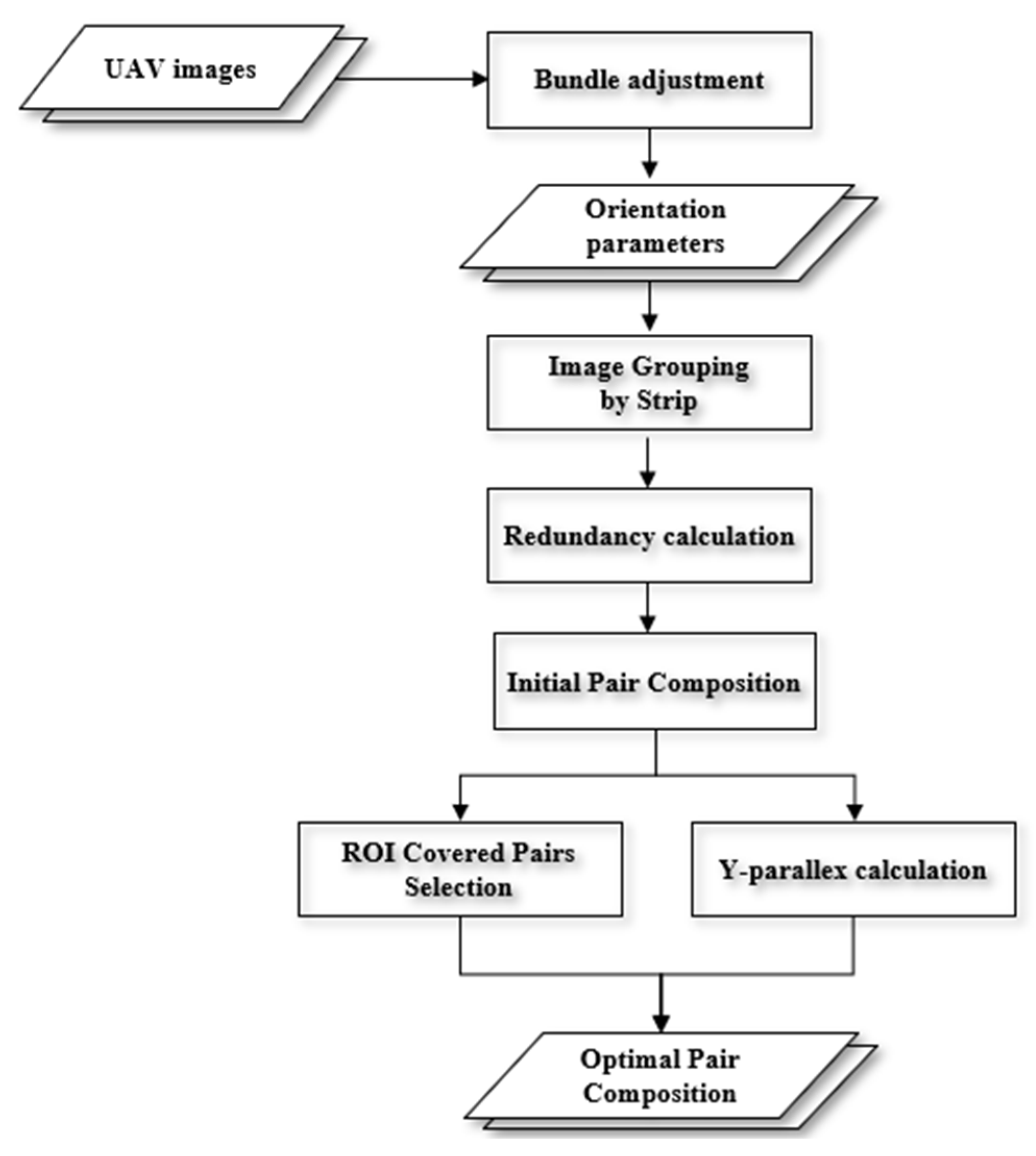
2. Proposed Method
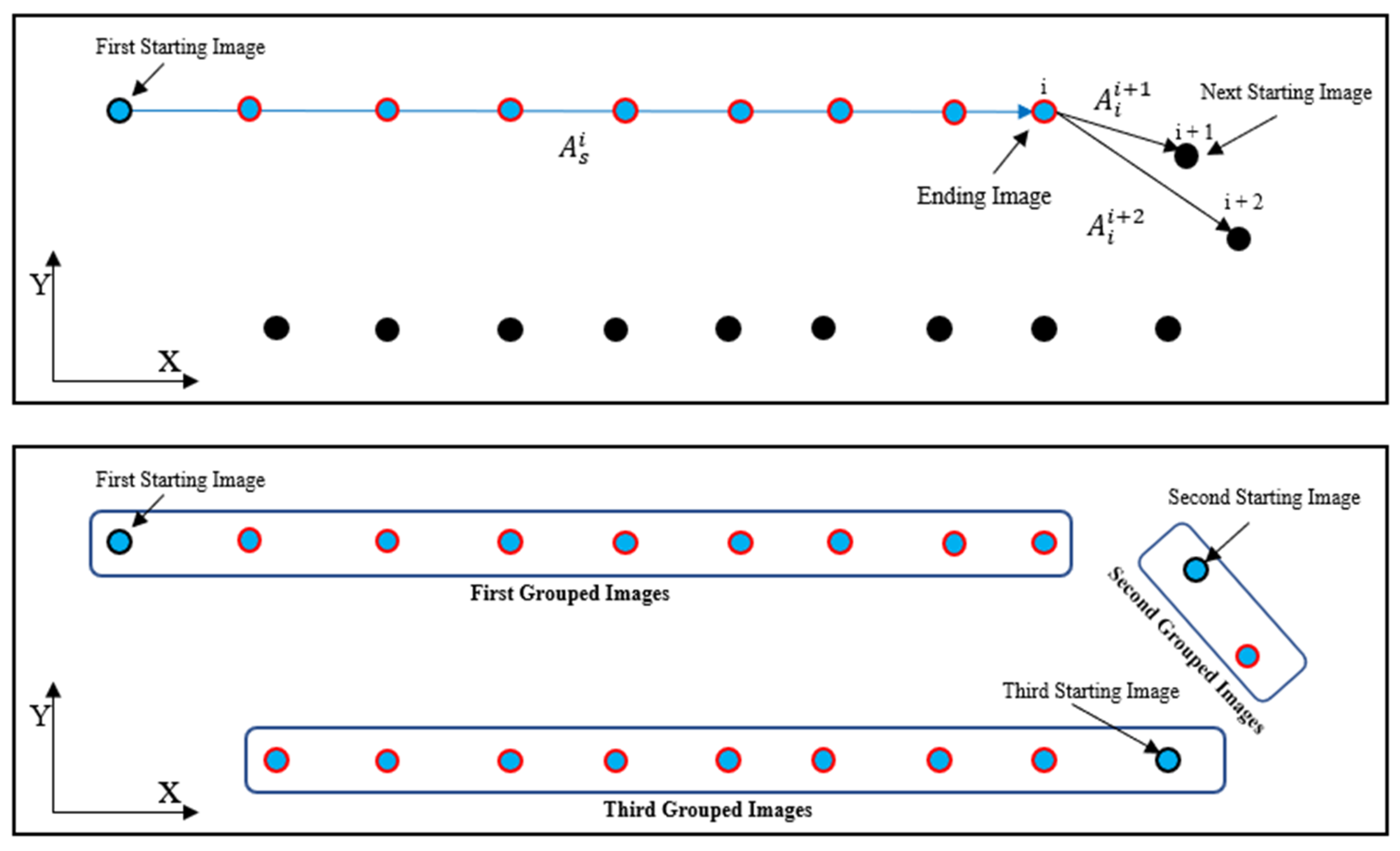
2.1. Image Grouping into Strips
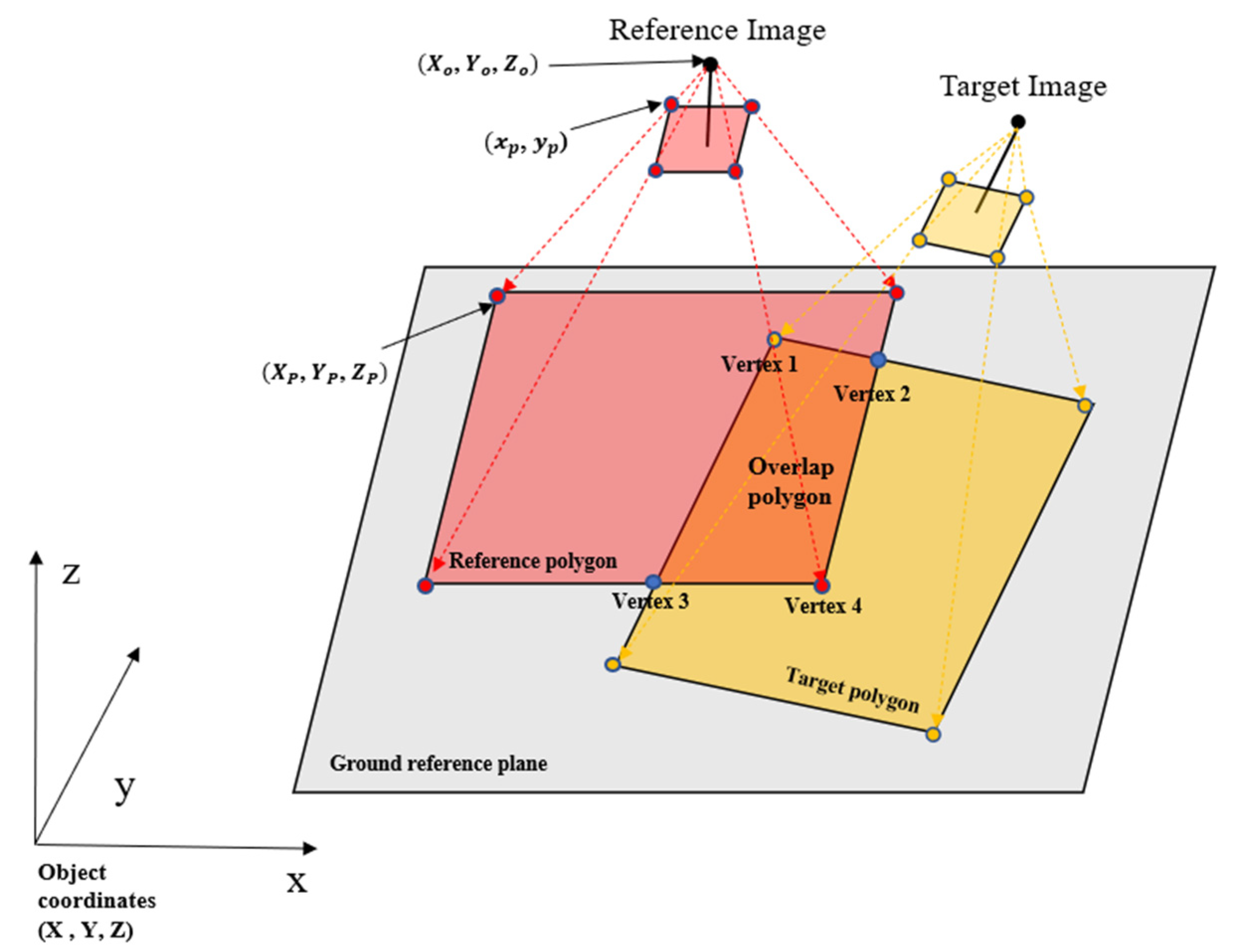
2.2. Initial Image Pair Composition
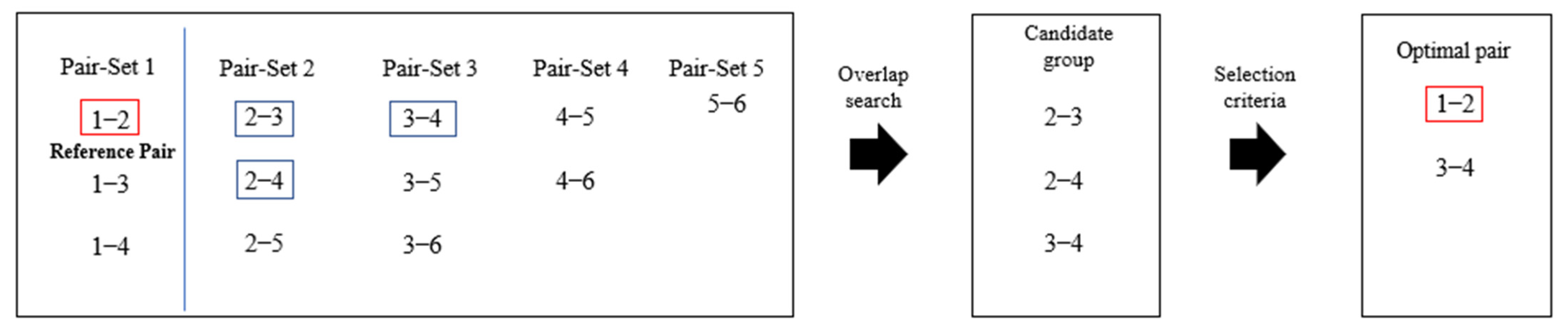
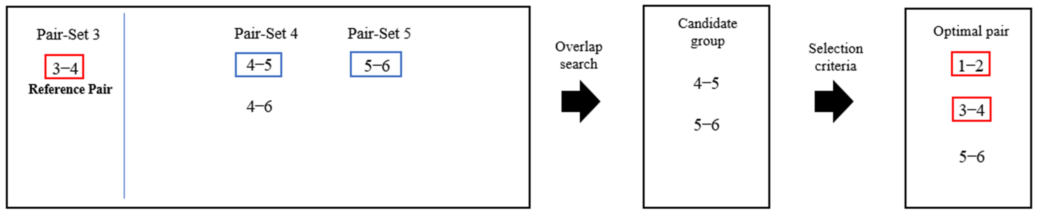
2.3. Optimal Pair Selection
3. Experiment Results and Discussion
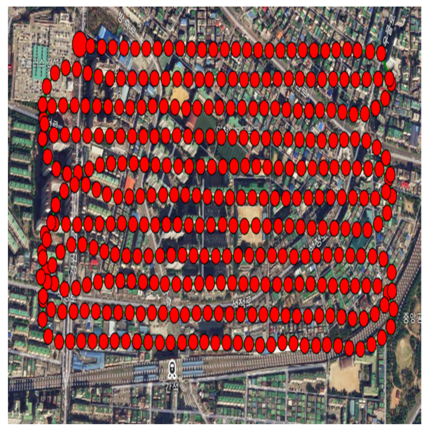
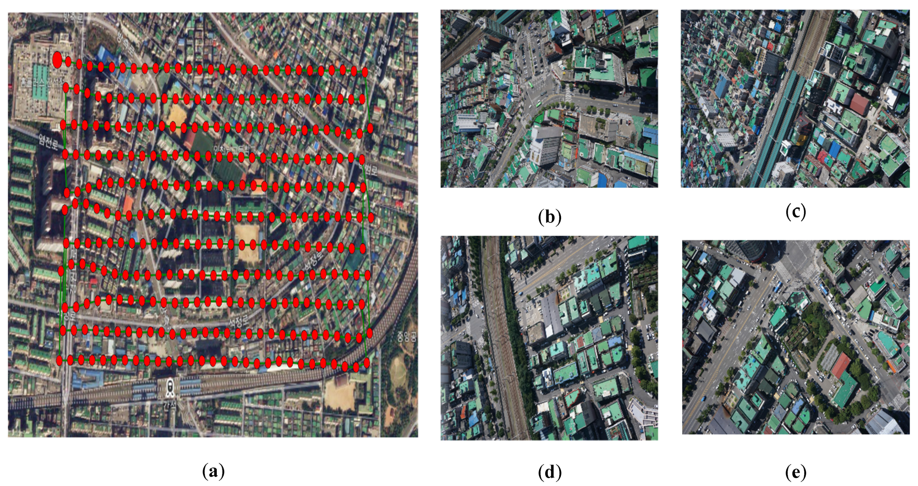
3.1. Study Area and Data
3.2. Image Grouping and Initial-Pair Composition
3.3. Optimal Image-Pair Selection
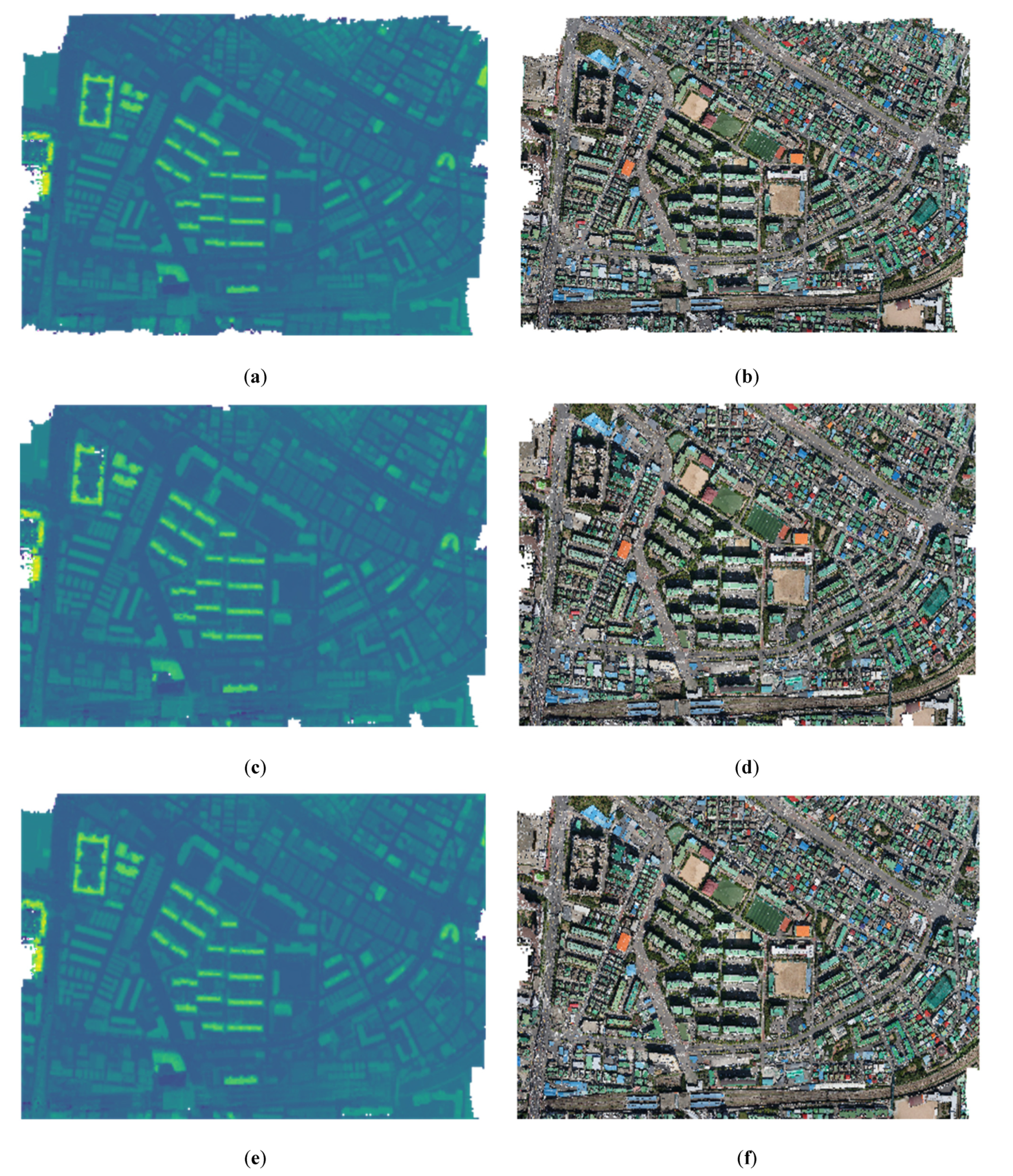
3.4. Performance of Stereoscopic Processing
4. Conclusions
Author Contributions
Funding
Conflicts of Interest
References
- Park, Y.; Jung, K. Availability evaluation for generation of geospatial information using fixed wing UAV. J. Korean Soc. Geospat. Inform. Syst. 2014, 22–24, 159–164. [Google Scholar]
- Lim, P.C.; Seo, J.; Son, J.; Kim, T. Feasibility study for 1:1000 scale map generation from various UAV images. In Proceedings of the International Symposium on Remote Sensing, Taipei, Taiwan, 17–19 April 2019. Digitally available on CD. [Google Scholar]
- Radford, C.R.; Bevan, G. A calibration workflow for prosumer UAV cameras. Int. Arch. Photogram. Remote Sens. Spat. Inform. Sci. 2019, XLII-2/W13, 553–558. [Google Scholar] [CrossRef] [Green Version]
- Rhee, S.; Hwang, Y.; Kim, S. A study on point cloud generation method from UAV image using incremental bundle adjustment and stereo image matching technique. Korean J. Remote Sens. 2019, 34, 941–951. [Google Scholar]
- Zhou, Y.; Rupnik, E.; Meynard, C.; Thom, C.; Pierrot-Deseilligny, M. Simulation and Analysis of Photogrammetric UAV Image Blocks—Influence of Camera Calibration Error. Remote Sens. 2019, 12, 22. [Google Scholar] [CrossRef] [Green Version]
- Cucci, D.A.; Rehak, M.; Skaloud, J. Bundle adjustment with raw inertial observations in UAV applications. ISPRS J. Photogram. Remote Sens. 2017, 130, 1–12. [Google Scholar] [CrossRef]
- Wohlfeil, J.; Grießbach, D.; Ernst, I.; Baumbach, D.; Dahlke, D. Automatic camera system calibration with a chessboard enabling full image coverage. Int. Arch. Photogramm. Remote Sens. Spat. Inf. Sci. 2019, 42, 1715–1722. [Google Scholar] [CrossRef] [Green Version]
- Choi, Y.; You, G.; Cho, G. Accuracy analysis of UAV data processing using DPW. J. Korean Soc. Geospat. Inform. Sci. 2015, 23, 3–10. [Google Scholar]
- Dai, Y.; Gong, J.; Li, Y.; Feng, Q. Building segmentation and outline extraction from UAV image-derived point clouds by a line growing algorithm. Int. J. Digit. Earth 2017, 10, 1077–1097. [Google Scholar] [CrossRef]
- Kim, J.I.; Kim, T.; Shin, D.; Kim, S. Fast and robust geometric correction for mosaicking UAV images with narrow overlaps. Int. J. Remote Sens. 2017, 38, 2557–2576. [Google Scholar] [CrossRef]
- Kim, J.I.; Hyun, C.U.; Han, H.; Kim, H.C. Evaluation of Matching Costs for High-Quality Sea-Ice Surface Reconstruction from Aerial Images. Remote Sens. 2019, 11, 1055. [Google Scholar] [CrossRef] [Green Version]
- Maini, P.; Sujit, P.B. On cooperation between a fuel constrained UAV and a refueling UGV for large scale mapping applications. In Proceedings of the International Conference on Unmanned Aircraft Systems, Denver, CO, USA, 9–12 June 2015; pp. 1370–1377. [Google Scholar]
- Shin, J.; Cho, Y.; Lim, P.; Lee, H.; Ahn, H.; Park, C.; Kim, T. Relative Radiometric Calibration Using Tie Points and Optimal Path Selection for UAV Images. Remote Sens. 2020, 12, 1726. [Google Scholar] [CrossRef]
- Brown, M.; Lowe, D.G. Automatic panoramic image stitching using invariant features. Int. J. Comp. Vis. 2017, 74, 59–73. [Google Scholar] [CrossRef] [Green Version]
- Kim, J.I. Development of a Tiepoint Based Image Mosaicking Method Considering Imaging Characteristics of Small UAV. Ph.D. Thesis, Inha University, Incheon, Korea, 2017. [Google Scholar]
- Kim, J.I.; Kim, T. Precise rectification of misaligned stereo images for 3D image generation. J. Broadcast Eng. 2012, 17, 411–421. [Google Scholar] [CrossRef]
- Kim, J.I.; Kim, H.C.; Kim, T. Robust Mosaicking of Lightweight UAV Images Using Hybrid Image Transformation Modeling. Remote Sens. 2020, 12, 1002. [Google Scholar] [CrossRef] [Green Version]
- Jung, J.; Kim, T.; Kim, J.; Rhee, S. Comparison of Match Candidate Pair Constitution Methods for UAV Images Without Orientation Parameters. Korean. J. Remote Sens. 2016, 32, 647–656. [Google Scholar]
- Son, J.; Lim, P.C.; Seo, J.; Kim, T. Analysis of bundle adjustments and epipolar model accuracy according to flight path characteristics of UAV. Int. Arch. Photogram. Remote Sens. Spat. Inf. Sci. 2019, 607–612. [Google Scholar] [CrossRef] [Green Version]
- Jeong, J.; Kim, T. Analysis of dual-sensor stereo geometry and its positioning accuracy. Photogram. Eng. Remote Sens. 2014, 80, 653–661. [Google Scholar] [CrossRef]
- Jeong, J.; Yang, C.; Kim, T. Geo-positioning accuracy using multiple-satellite images: IKONOS, QuickBird, and KOMPSAT-2 stereo images. Remote Sens. 2015, 7, 4549–4564. [Google Scholar] [CrossRef] [Green Version]
- Haines, E. Point in polygon strategies. Graph. Gems IV 1994, 994, 24–26. [Google Scholar]
- Yoon, W.; Kim, H.G.; Rhee, S. Multi point cloud integration based on observation vectors between stereo images. Korean J. Remote Sens. 2019, 35, 727–736. [Google Scholar]
- Lee, S.B.; Kim, T.; Ahn, Y.J.; Lee, J.O. Comparison of Digital Maps Created by Stereo Plotting and Vectorization Based on Images Acquired by Unmanned Aerial Vehicle. Sens. Mater. 2019, 31, 3797–3810. [Google Scholar] [CrossRef]


| Strip | Start Index of Image | End Index of Image | Number of Images | Number of Pair-Sets | Number of Pairs |
|---|---|---|---|---|---|
| 1 | 1 | 27 | 27 | 26 | 86 |
| 2 | 34 | 59 | 26 | 25 | 79 |
| 3 | 67 | 92 | 26 | 25 | 77 |
| 4 | 99 | 124 | 26 | 25 | 77 |
| 5 | 133 | 158 | 26 | 25 | 77 |
| 6 | 164 | 192 | 29 | 28 | 82 |
| 7 | 199 | 226 | 28 | 27 | 81 |
| 8 | 234 | 259 | 26 | 25 | 76 |
| 9 | 268 | 295 | 28 | 27 | 80 |
| 10 | 299 | 328 | 30 | 29 | 87 |
| 11 | 334 | 362 | 29 | 28 | 82 |
| Total Number | 301 | 290 | 884 | ||
| Pair-Set 1 | Pair-Set 2 | Pair-Set 3 | Pair-Set 4 | Pair-Set 5 | Pair-Set 6 | Pair-Set 7 |
| 1–2 (66, 0.6) | 2–3 (84, 1.0) | 3–4 (85, 0.7) | 4–5 (84, 0.4) | 5–6 (72, 1.0) | 6–7 (76, 0.6) | 7–8 (73, 0.8) |
| 1–3 (51, 0.7) | 2–4 (68, 1.0) | 3–5 (73, 0.7) | 4–6 (58, 1.1) | 5–7 (51, 0.7) | 6–8 (50, 0.9) | 7–9 (43, 0.8) |
| 1–4 (38, 1.1) | 2–5 (57, 1.1) | 3–6 (46, 1.2) | 4–7 (39, 0.6) | 5–8 (30, 1.6) | 6–9 (22, 1.0) | 7–10 (22, 1.0) |
| 1–5 (28, 3.2) | 2–6 (36, 2.4) | 3–7 (26, 0.8) | ||||
| Pair-Set 8 | Pair-Set 9 | Pair-Set 10 | Pair-Set 11 | Pair-Set 12 | Pair-Set 13 | Pair-Set 14 |
| 8–9 (69, 0.8) | 9–10 (77, 0.7) | 10–11 (74, 3.8) | 11–12 (72, 0.5) | 12–13 (81, 0.4) | 13–14 (76, 0.4) | 14–15 (78, 0.7) |
| 8–10 (47, 1.0) | 9–11 (54, 2.9) | 10–12 (49, 3.7) | 11–13 (58, 0.5) | 12–14 (59, 0.5) | 13–15 (57, 0.7) | 14–16 (51, 0.8) |
| 8–11 (27, 0.8) | 9–12 (30, 2.8) | 10–13 (35, 3.3) | 11–14 (39, 0.7) | 12–15 (40, 0.8) | 13–16 (33, 0.8) | 14–17 (29, 1.0) |
| Pair-Set 15 | Pair-Set 16 | Pair-Set 17 | Pair-Set 18 | Pair-Set 19 | Pair-Set 20 | Pair-Set 21 |
| 15–16 (72, 0.4) | 16–17 (76, 0.5) | 17–18 (76, 0.7) | 18–19 (79, 0.6) | 19–20 (72, 0.5) | 20–21 (78, 0.6) | 21–22 (75, 0.8) |
| 15–17 (48, 0.6) | 16–18 (53, 0.7) | 17–19 (58, 1.1) | 18–20 (53, 1.1) | 19–21 (54, 0.7) | 20–22 (63, 0.8) | 21–23 (56, 1.5) |
| 15–18 (26, 0.6) | 16–19 (35, 0.9) | 17–20 (32, 1.9) | 18–21 (36, 1.1) | 19–22 (38, 0.9) | 20–23 (36, 1.6) | 21–24 (37, 1.1) |
| 18–22 (20, 2.2) | 20–24 (25, 0.7) | |||||
| Pair-Set 22 | Pair-Set 23 | Pair-Set 24 | Pair-Set 25 | Pair-Set 26 | ||
| 22–23 (69, 1.3) | 23–24 (75, 1.0) | 24–25 (71, 0.7) | 25–26 (70, 1.7) | 26–27 (74, 1.1) | ||
| 22–24 (61, 0.7) | 23–25 (48, 0.9) | 24–26 (48, 1.7) | 25–27 (48, 1.2) | |||
| 22–25 (32, 0.8) | 23–26 (33, 2.0) | 24–27 (25, 1.8) |
| Strip | Case 1. Adjacent—Pair Selection | Case 2. Minimum—Pair Selection | Case 3. Most Accurate—Pair Selection | |||
|---|---|---|---|---|---|---|
| Number of Pairs | Y-Parallax (Pixels) | Number of Pairs | Y-Parallax (Pixels) | Number of Pairs | Y-Parallax (Pixels) | |
| 1 | 26 | 0.80 | 9 | 0.90 | 13 | 0.61 |
| 2 | 25 | 0.61 | 9 | 0.56 | 12 | 0.51 |
| 3 | 25 | 0.70 | 8 | 0.88 | 13 | 0.55 |
| 4 | 25 | 0.61 | 11 | 0.76 | 14 | 0.53 |
| 5 | 25 | 0.77 | 7 | 0.80 | 12 | 0.61 |
| 6 | 28 | 0.70 | 10 | 0.60 | 12 | 0.50 |
| 7 | 27 | 0.74 | 9 | 0.65 | 14 | 0.58 |
| 8 | 25 | 0.75 | 9 | 0.72 | 15 | 0.64 |
| 9 | 27 | 0.75 | 10 | 0.80 | 15 | 0.66 |
| 10 | 29 | 0.74 | 10 | 0.55 | 15 | 0.51 |
| 11 | 28 | 0.71 | 9 | 0.84 | 12 | 0.63 |
| Avg | 26 | 0.71 | 9 | 0.73 | 13 | 0.58 |
| Total | 290 | - | 101 | - | 148 | - |
| Type of Product | Case 1. Adjacent—Pair Selection | Case 2. Minimum—Pair Selection | Case 3. Most Accurate—Pair Selection |
|---|---|---|---|
| Stereo matching | 100 min | 38 min | 57 min |
| DSM and Ortho-mosaic | 15 min | 7 min | 9 min |
| Total processing time | 115 min | 45 min | 66 min |
| Accuracy | Case 1. Adjacent Pair Selection | Case 2. Minimum Pair Selection | Case 3. Most Accurate Pair Selection | |||
|---|---|---|---|---|---|---|
| Horizontal (cm) | Vertical (cm) | Horizontal (cm) | Vertical (cm) | Horizontal (cm) | Vertical (cm) | |
| Model | 8.4 | 25.2 | 5.5 | 22.8 | 6.1 | 7.4 |
| Check | 8.2 | 18.3 | 7.2 | 24.2 | 5.9 | 7.5 |
| Study Region | Type of UAV | Number of Strip | Number of Input Images | Number of Most Accurate Pairs | Y-Parallax RMSE (Pixel) |
|---|---|---|---|---|---|
| Agricultural | Fixed-wings | 6 | 59 | 18 | 0.84 |
| Costal | Rotary-wings | 6 | 95 | 26 | 0.88 |
| Agricultural | Rotary-wings | 6 | 51 | 15 | 0.55 |
Publisher’s Note: MDPI stays neutral with regard to jurisdictional claims in published maps and institutional affiliations. |
© 2021 by the authors. Licensee MDPI, Basel, Switzerland. This article is an open access article distributed under the terms and conditions of the Creative Commons Attribution (CC BY) license (https://creativecommons.org/licenses/by/4.0/).
Share and Cite
Lim, P.-c.; Rhee, S.; Seo, J.; Kim, J.-I.; Chi, J.; Lee, S.-b.; Kim, T. An Optimal Image–Selection Algorithm for Large-Scale Stereoscopic Mapping of UAV Images. Remote Sens. 2021, 13, 2118. https://0-doi-org.brum.beds.ac.uk/10.3390/rs13112118
Lim P-c, Rhee S, Seo J, Kim J-I, Chi J, Lee S-b, Kim T. An Optimal Image–Selection Algorithm for Large-Scale Stereoscopic Mapping of UAV Images. Remote Sensing. 2021; 13(11):2118. https://0-doi-org.brum.beds.ac.uk/10.3390/rs13112118
Chicago/Turabian StyleLim, Pyung-chae, Sooahm Rhee, Junghoon Seo, Jae-In Kim, Junhwa Chi, Suk-bae Lee, and Taejung Kim. 2021. "An Optimal Image–Selection Algorithm for Large-Scale Stereoscopic Mapping of UAV Images" Remote Sensing 13, no. 11: 2118. https://0-doi-org.brum.beds.ac.uk/10.3390/rs13112118