
Predicting Table Beet Root Yield with Multispectral UAS Imagery


1
Chester F. Carlson Center for Imaging Science, Rochester Institute of Technology, Rochester, NY 14623, USA
2
Plant Pathology & Plant-Microbe Biology Section, School of Integrative Plant Science, Cornell AgriTech, Cornell University, Geneva, NY 14456, USA
3
Love Beets USA, Rochester, NY 14606, USA
*
Author to whom correspondence should be addressed.
Remote Sens. 2021, 13(11), 2180; https://0-doi-org.brum.beds.ac.uk/10.3390/rs13112180
Submission received: 9 April 2021
/
Revised: 31 May 2021
/
Accepted: 31 May 2021
/
Published: 2 June 2021
(This article belongs to the Special Issue Advances in Remote Sensing for Crop Monitoring and Yield Estimation)
Abstract
:Timely and accurate monitoring has the potential to streamline crop management, harvest planning, and processing in the growing table beet industry of New York state. We used unmanned aerial system (UAS) combined with a multispectral imager to monitor table beet (Beta vulgaris ssp. vulgaris) canopies in New York during the 2018 and 2019 growing seasons. We assessed the optimal pairing of a reflectance band or vegetation index with canopy area to predict table beet yield components of small sample plots using leave-one-out cross-validation. The most promising models were for table beet root count and mass using imagery taken during emergence and canopy closure, respectively. We created augmented plots, composed of random combinations of the study plots, to further exploit the importance of early canopy growth area. We achieved a R2 = 0.70 and root mean squared error (RMSE) of 84 roots (~24%) for root count, using 2018 emergence imagery. The same model resulted in a RMSE of 127 roots (~35%) when tested on the unseen 2019 data. Harvested root mass was best modeled with canopy closing imagery, with a R2 = 0.89 and RMSE = 6700 kg/ha using 2018 data. We applied the model to the 2019 full-field imagery and found an average yield of 41,000 kg/ha (~40,000 kg/ha average for upstate New York). This study demonstrates the potential for table beet yield models using a combination of radiometric and canopy structure data obtained at early growth stages. Additional imagery of these early growth stages is vital to develop a robust and generalized model of table beet root yield that can handle imagery captured at slightly different growth stages between seasons.
1. Introduction
New York is a sentinel center of production for table beet (Beta vulgaris spp. vulgaris: Family Chenopodiaceae) in the USA, ranking second behind Wisconsin [1], and is undergoing exponential industry growth. The table beet industry in New York is diverse in enterprise size and scale, ranging from small, diversified growers that supply farm markets and roadside stands to broad-acre fields up to approximately 45 ha in size. Broad-acre production is for processing into cans and jars, direct fresh market sales, and feedstock as value-added beet products, such as snack packs and juices. The growth of the industry is fueled by an enhanced awareness of the health benefits of consuming table beets and beet-based products. These well-documented effects range from nutritional intervention to disease mitigation [2]. The most commonly reported physiological changes associated with table beet consumption include improvements in cardiovascular health and sugar metabolism attributed to the rich source of dietary nitrate [3,4], the antioxidant and anti-inflammatory effects of betalains [5], and the potential to improve stamina in exercise [6]. Red table beets are also grown as the main source of betacyanins, which are the basis of coloring used in food products [7].
Crop yield is generally defined as the ratio of the mass of a harvested crop to the physical area of land used for production [8]. Depending on the crop and its end market, a farmer may need to consider multiple yield parameters relevant to their potential financial returns. In the case of table beets, the number of roots, and the percentage of roots falling in specific shoulder diameter ranges are of particular interest, in addition to the standard kilograms per hectare yield. Logistically, table beet roots of various sizes are used for different products, with distinct processing and packaging needs. This motivates the stakeholders, hoping to meet yield and beet diameter distribution targets, to obtain early crop management inputs which may be relevant to strategic planning, a reduction in waste, maximization of financial gain, and potential within-season intervention.
Precision agriculture methods have been developed to monitor and manage crops at small scales in the last several decades, focusing on in-field applications of farm inputs, rather than prescribing uniform treatments across an entire field [9]. The utility of crop yield modeling for management is to provide farmers with clearly actionable decision-making information concerning their fields, with model inputs sourced from data obtained with minimal cost and effort [10]. These can be data pertaining to the in-field spatial soil, water, nutrient, and topographic conditions for the crop, and local weather information. While such inputs pertain to the ingredients for a variety of plant growth outcomes, we can also use satellite, airborne, or unmanned aerial system (UAS) imagery to incorporate the radiometric and structural properties of the resulting crop canopies. Applications of remote sensing include biomass and yield estimation, monitoring of vegetation vigor, drought stress, and crop phenological development [11]. The most thorough assessment of in-field crop conditions would ideally contain all sources of information related to the base determinants of crop growth, supplemented with remote sensing imagery. However, in situ observations can be costly, time consuming, and destructive, thus prohibiting broader adoption [12]. An UAS equipped with an affordable multispectral camera, on the other hand, can rapidly and non-destructively obtain full-field imagery for use as predictor variables in crop yield modeling.
UAS and airborne multispectral imagery and vegetation indices derived from combinations of two or more select bands, to enhance the contribution of vegetation properties, have been used for yield prediction in a variety of crop scenarios, including rice [13,14], maize/corn [15,16] and wheat [17]. For example, Zhou et al. [18] found that indices from multispectral imagery were correlated (R2 > 0.7) with rice grain yield at various growth stages. Models using data from different epochs may rely on different vegetation indices and reflectance bands as primary inputs, as found in similar modeling studies of corn [16] and sugar beet [19] yield. A multitemporal approach can also allow for the determination of an optimal timing and growth stage for imagery collection [18,20].
Remote sensing of root crops, including sugar beet (also B. vulgaris ssp. vulgaris), has also shown potential for success of UAS-based yield estimation of table beets. Bu et al. [21] found that RapidEye satellite imagery could be used to predict sugar beet root yield comparably to common ground-based sensors, but concluded that a UAS sensing approach may be necessary due to the lack of available satellite imagery coinciding with clear skies. Olson et al. [19,20] more recently found that pairing of UAS-derived multispectral vegetation indices and canopy height can provide improved sugar beet yield predictions when compared to vegetation indices alone. Their modeling used imagery from multiple growth stages across two different seasons at two different sites. This study also found that the significance of canopy height diminished in seasons with lower rainfall, and modeling results of both vegetation indices and canopy height were inconsistent between growing seasons and sites. The predictive ability of both vegetation indices, canopy height, and a combination thereof was found to be significant only in certain growth stages and the optimal growth stage was not always consistent between the two seasons and sites [20]. The best sugar beet root yield model was for combined NDVI and crop height at one site in 2017, with an , during the sugarbeet V10 growth stage (approximately 28 June in western Minnesota) [19].
Canopy area is especially important for imagery obtained at early growth stages before the neighboring canopies have merged. Canopy height is also important but can be difficult to assess before the plants are several centimeters in height, depending on the ground sample distance (GSD) of the imagery. Overall, the early stages are well suited to assess the vigor of early crop growth via both the average radiometric properties of the canopy and the extent of the canopy growth in terms of canopy area and/or height [22,23,24,25].
In this work, we exclusively investigate the predictive power of UAS multispectral imagery for table beet yield components (root mass, count, and shoulder diameter size distributions) at harvest. This is a challenging research task, since, for many crops with aboveground fruits, the health or yield can be directly estimated with imagery, but for root vegetables, we can only infer their yield with imagery exclusively via their canopy structure and reflectance. We build on previous work by creating area-augmented data from our experimental plots in order to exploit the importance of structural metrics derived from imagery and to evaluate model performance on independent data.
2. Materials and Methods
2.1. Study Area
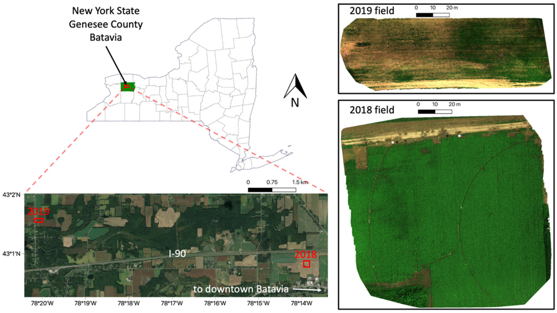
The Rochester Institute of Technology UAS and Cornell University agronomy teams collected multispectral imagery and ground truth agronomic data from table beet fields located in Batavia, New York, USA during July and August of 2018 and 2019 (see Figure 1). The commercial fields contained table beet cv. Merlin, planted in accordance with typical industry management practices, i.e., twin rows with approximately 10 cm between-plant spacing and ~60 cm between-row spacing.
2.2. Data Collection
Fifty 3 m long plots were marked soon after crop emergence (5 July 2018), as well as 20, 1.5 m long plots during the following season (15 July 2019). Four and two data collections of agronomic ground truth and UAS canopy reflectance data were collected in 2018 and 2019, respectively. An additional ground truth harvest collection, without imagery, was also conducted in 2019. Crop stands were assessed for both years by counting the plants in the entire length of each of the double-row plots on each occasion. Canopy reflectance imagery were obtained as close as possible to the ground truth collection dates via a DJI Matrice 100 UAS vehicle, mounted with a MicaSense RedEdge-M five-band multispectral visible-near-infrared (VNIR) camera system. Due to instrument availability, canopy reflectance imagery was obtained using a DJI Matrice 600 UAS equipped with a Headwall Photonics Nano-Hyperspec imaging spectrometer (272 spectral bands; 400–1000 nm) for the second observation in 2018, in lieu of the multispectral imagery. At harvest, in addition to plant/root counts, a number of yield parameters were collected in the 2018 season by hand removal of all plants within the plots (Table 1). These included root number, root mass (kg), root shoulder diameters (mm), and the dry weight of the foliage separated from the roots. Foliage was weighed in the field and a subsample (approximately 10% of the total weight) was dried at 60 °C for 48 h to calculate dry weight. Roots over 20 mm in diameter were counted and weighed, and returned to Geneva, NY for storage at 10 °C for up to 10 days, until shoulder diameters were measured using digital calipers (Mitutoyo, USA). Only root count was conducted for the 2019 harvest.
The MicaSense RedEdge-M camera captured images in five narrowband spectral channels (blue, green, red, red edge, and near-infrared [26]; Table 2). The flight ground sample distances ranged from 0.5 to 10 cm/pixel. We down-sampled the hyperspectral imaging canopy reflectance spectra for each pixel to simulate the standard multispectral imagery for the second observation in 2018. We integrated the pixel spectra, multiplied with a Gaussian of peak central wavelength and full width at half maximum (FWHM) to down-sample the spectra (Table 2).
2.3. Data Preprocessing
We registered, orthorectified, and calibrated all UAS multispectral imagery obtained with the MicaSense camera using the Pix4D software (V.4.4.12) [27]. The software processing ingests the raw frames from each spectral band and outputs co-registered and radiometrically-corrected reflectance orthomosaics. GPS ground control points were deployed in the fields for manual identification of tie-points to verify and improve band and image registration.
The calibration procedure for the MicaSense camera uses sensor and image specific metadata parameters for conversion from raw digital counts to radiance (W/m2/sr/nm). These include parameters for a vignette correction function, radiometric calibration coefficients, sensor gain, exposure time, and black level values [28,29]. Additionally, the MicaSense camera was paired with a 5-band downwelling light sensor (DLS 2) to capture the downwelling radiance in sync with the radiance imagery of the crop canopy [30]. The Pix4D software uses the primary camera parameters, sun irradiance measured with DLS, and sun angle from the DLS inertial measurement unit for radiometric correction [29]. We then stacked the resulting reflectance mosaics for each band into one multispectral image, using ENVI software (V.5.5) [31].
The 2018 observations with hyperspectral imagery were pre-processed for orthorectification and radiance calibration/conversion using Headwall’s Hyperspec III SpectralView software [32]. The spectral imagery captured black, dark gray, light gray, and white calibration panels deployed on the north side of the 2018 site. We extracted the calibration panel spectra using ENVI (V.5.5 [31]). The panels have well-characterized ground truth reflectance spectra that were used to convert the pre-processed radiance flight imagery into reflectance. We used the Empirical Line Method (ELM) tool in ENVI [33] to determine the relationship between the calibration panel UAS radiance spectra and their true reflectance spectra and determined linear coefficients to convert between radiance and reflectance at each wavelength. This process removes both solar irradiance and atmospheric path radiance.
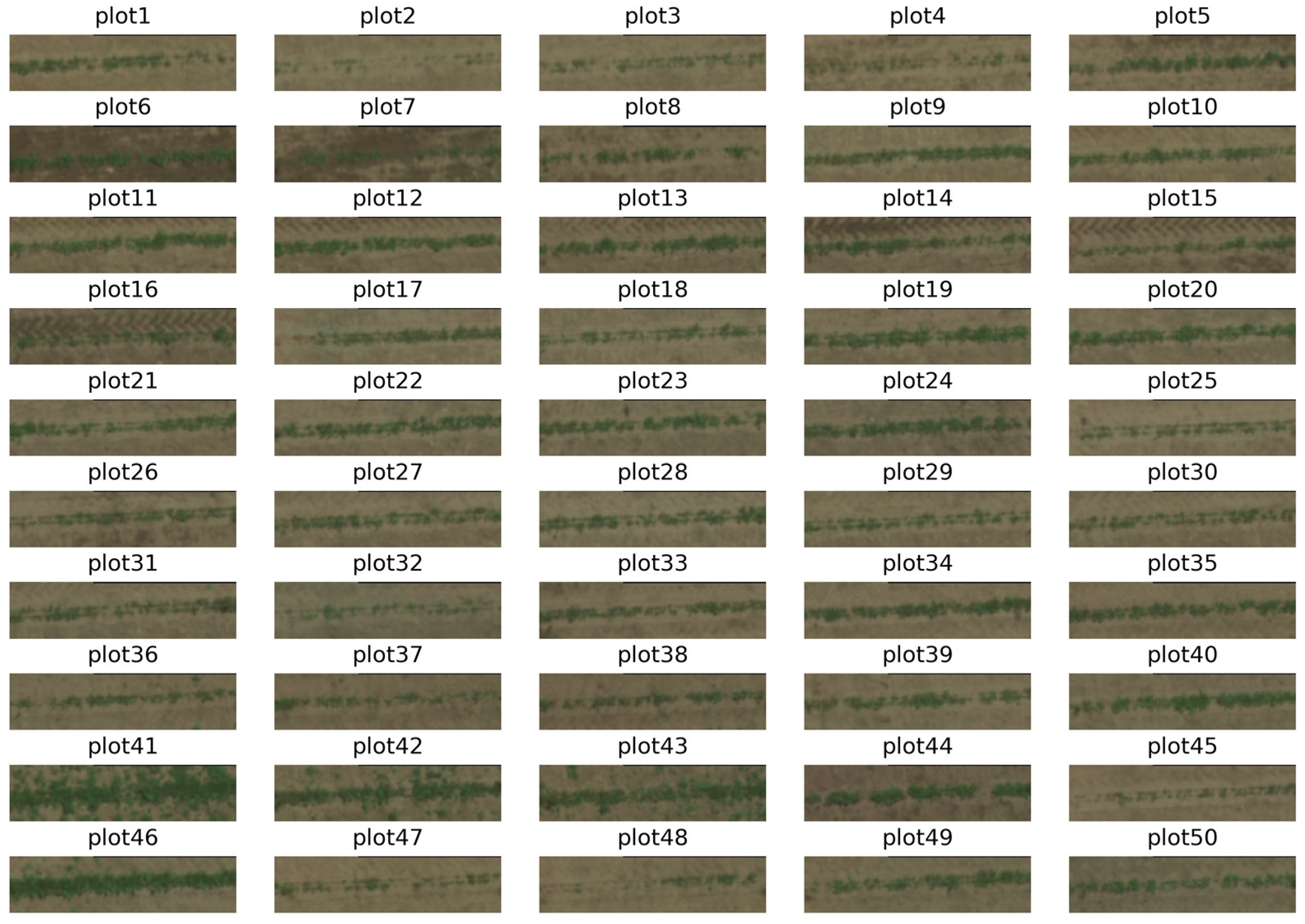
Plots in the field were marked with red plates to rapidly locate and define regions of interest (ROIs) for each plot using ENVI. The plots differ in pixel dimensions for each set of imagery, depending on the ground sample distance of the UAS-based MicaSense imagery. We extracted 5-band plot images from each of the ROIs and used the Spectral Python library SPy (V.0.20) [34] to import the ENVI-formatted plot images to NumPy Arrays in Python for further analysis. Figure 2 displays a sample of the extracted plot imagery from the 9 July 2018 flight (shortly following crop emergence). We noted that plots 41, 42, 43, and 46 exhibited substantial weed growth at this stage and were removed from the analysis. Additionally, plot 27 had an anomalously high recorded foliage mass (>2× of other plots) and was removed as an outlier/erroneous recording. The next step required accurate identification of vegetation pixels for further analysis.
2.4. Canopy Pixel Segmentation
Several methods may be used to identify the pixels containing vegetation in plot imagery. We clearly distinguished the crop canopy from background soil, prior to the growth reaching a state of overlapped row canopies, due to the high spatial resolution of the UAS imagery. Common classification practices include applying an appropriate threshold to the spectral angle map (SAM) of an endmember spectrum [35] or using k-means clustering to identify and classify spectral endmembers [36]. However, band reflectance can change substantially with canopy growth, causing these methods to provide inconsistent results amongst the various datasets. We thus opted for a relatively simple VI threshold to identify vegetation pixels in each plot. Similar to Barzin et al. [16], we determined that while a Normalized Difference Vegetation Index (NDVI) threshold is commonly used for soil masking [37,38], it is not capable of producing a consistent result amongst the imagery from varying growth stages using a single threshold value. We used the triangular vegetation index (TVI), because the TVI of the canopy exhibited a limited variation over the cropping season compared to NDVI.
The traditional formula for TVI, introduced by Broge and Leblanc [39], incorporates the green, red, and NIR bands as:
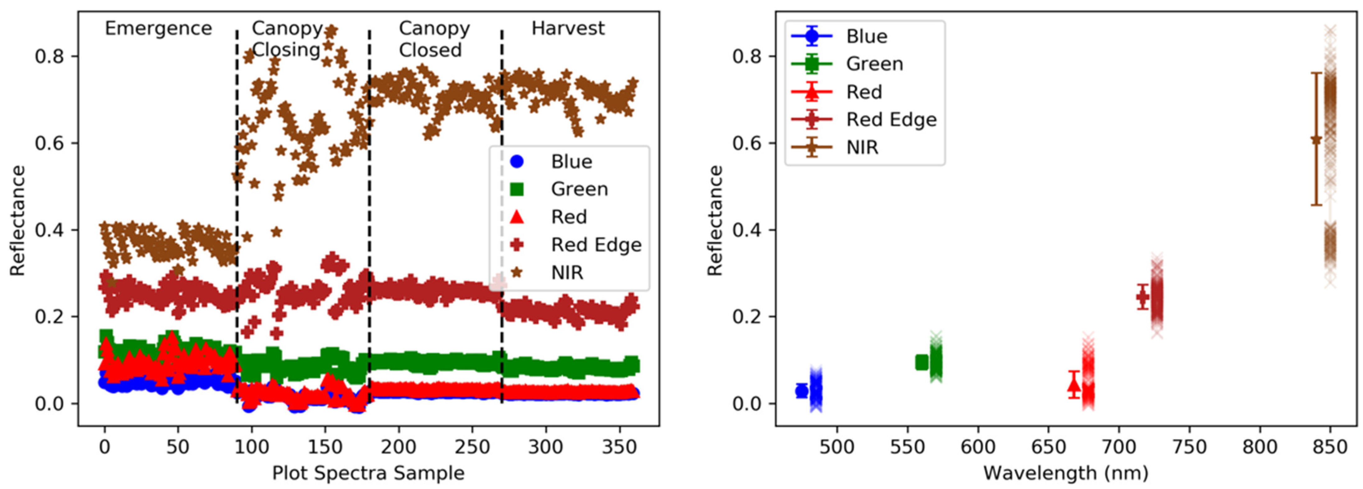
with reflectances = 550 nm, = 670 nm, and = 750 nm. This index essentially measures the area of the triangle, as defined by the peak green and red absorption trough, due to chlorophyll absorption, and the NIR plateau (inter-cellular leaf structure) in vegetation spectra [39]. We used the green, red, and red edge bands for vegetation classification (Table 2). The traditional TVI values are, therefore, expected to represent an increase in the triangular area as the canopy grows and NIR reflectance increases with more layers of vegetation. We chose to use the red edge band, instead of NIR, in order to limit the difference in the index between growth stages. The median reflectance for each band in all plot canopy imagery from 2018 are shown in Figure 3 (left) along with the complete average spectra (right). The canopy near-infrared reflectance is clearly the most variable throughout the growing season. The red edge band reflectance observed here only decreases slightly over the cropping season, as the red edge inflection point shifts to longer wavelengths with an increase in vegetation density [40]. This choice is convenient for the purpose of classification, since it allows use of a consistent threshold for every dataset. Other common indices, like NDVI, increase for canopy-level sensing throughout the growing season and require an adjustment to the threshold for each dataset to consistently classify all vegetation appropriately.
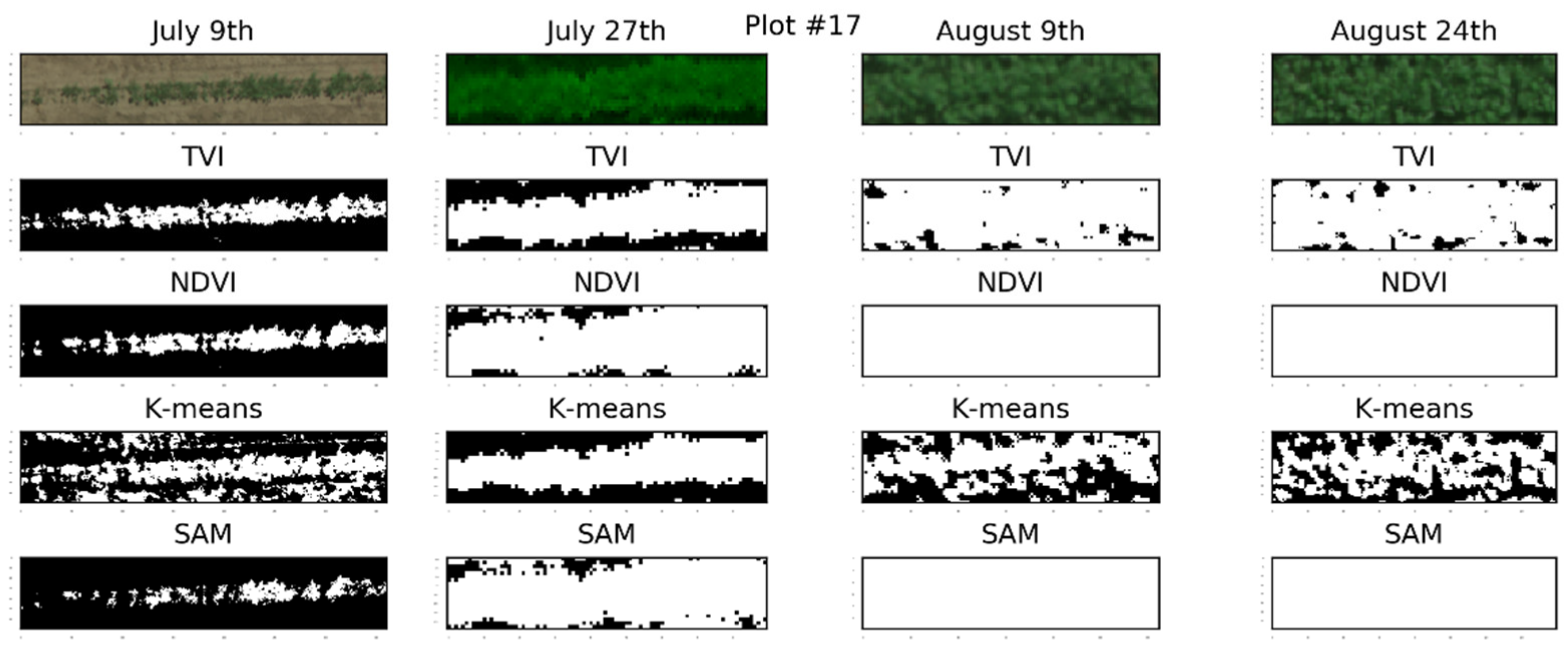
We included a comparison of the TVI threshold, SAM, k-means, and NDVI threshold methods on a sample plot over the course of the 2018 season to further reinforce our choice of the modified TVI for classification (Figure 4). The plot’s RGB composite and vegetation classification masks of each method are shown for each growth stage. The k-means and SAM masks were determined using the kmeans and msam [35] functions in the SPy library. The NDVI and SAM methods both classified the entire plot image as vegetation in the two final observations, but a stricter (higher) threshold for either method failed to classify the first observation’s vegetation pixels, due to the less-developed canopy. The k-means method is strongly dependent on the number of clusters chosen. In the later observations, it was optimal to use fewer clusters, because vegetation covered nearly the entire plot area, resulting in less spectral diversity. However, in early observations there was more variation in the plot image due to increased soil visibility. The image from 9 July 2018 required at least three clusters to properly classify only vegetation cover as actual vegetation. Thus, these three methods failed to classify the plot imagery of all four growth stages using a standard set of method parameters. Only the TVI threshold effectively classified all four growth stage images with a single threshold value for all four sets of imagery.
2.5. Feature Choice
Using the vegetation classification masks for each plot, we calculated a range of statistical and morphological features. To avoid overfitting issues caused by small sample sizes with high dimensionality [41], we limited our study to individual reflectance bands or biophysically-sensible VI features and single radiometric features paired with canopy area. We tested only VIs known to exhibit a priori phenological correlations with crop vigor, and from these constructed our final models only with those features exhibiting optimal posteriori correlations.
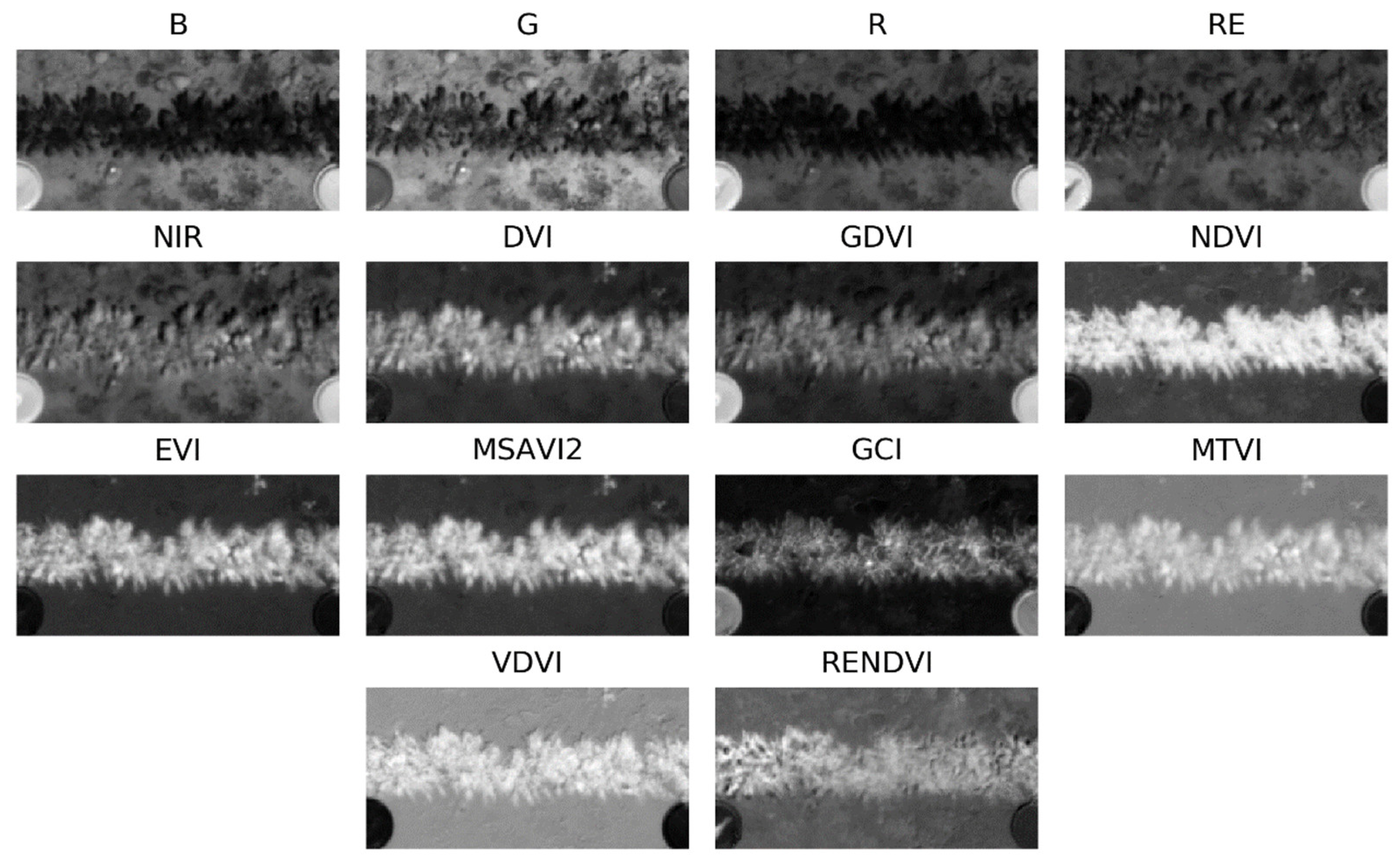
In addition to the five-band multispectral imagery, we calculated several VI images for each plot (Table 3; Figure 5). The indices used here were specifically chosen to capture different aspects of the plots’ spectra via incorporation of different combinations of the five camera bands. The basic Difference Vegetation Index (DVI) effectively separates the vegetation from the soil, but is sensitive to background soil reflectance [42]. We also included the similar Green Difference Vegetation Index (GDVI), designed for predicting nitrogen requirements in corn [43]. The most commonly-used vegetation index, NDVI, is related to canopy structure, Leaf Area Index (LAI), and photosynthesis [44], but is adversely sensitive to the background soil, atmospheric conditions, and shadowing. The Enhanced Vegetation Index (EVI) [45] attempts to correct for the soil and atmospheric effects in NDVI and offers more contrast in developed canopies, where NDVI may saturate due to a higher Leaf Area Index (LAI). The Modified Soil Adjusted Vegetation Index 2 (MSAVI2) [46] reduces noise due to soil and increases the dynamic range of the canopy signal, while the Green Chlorophyll Index (GCI) provides a better relation to chlorophyll content than NDVI [47]. The Modified Triangular Vegetation Index (MTVI), used for LAI estimation [48], is slightly different from the TVI we used earlier for vegetation classification, effectively swapping the NIR band for the red edge. We included the Visible-Band Difference Vegetation Index (VDVI) [49], which incorporates the blue, green, and red channels, to assess the effectiveness of using only visible channels. Finally, we included the Red Edge Normalized Difference Vegetation Index (RENDVI) [50] to capture variation in the vegetation spectra along the red edge.
We next determined the median reflectance of each band and median value of each VI for the vegetation-classified pixels in each plot. Although the pixel reflectance of each band did not deviate significantly from a Gaussian distribution, we used the median in lieu of the mean to eliminate the potential of an anomalous pixel skewing a plot’s reflectance or index values. We calculated the physical area of vegetation pixels for each plot, by multiplying the number of TVI > 7.5 threshold vegetation-classified pixels by the squared ground sampling distance. This yielded 15 total features (five bands, nine indices, and one area) for each plot to be used in data analysis for each growth stage imagery set.
2.6. Data Analysis
We investigated multiple linear regression (MLR) models using individual radiometric features combined with canopy area to model the various yield parameters with datasets from each growth stage. We used leave-one-out cross-validation (LOOCV) and for each MLR model (scikit-learn version 0.21.3) to determine the best-performing growth stage and radiometric feature for each yield component. We also summarize LOOCV results for individual feature linear models of canopy area and the best-performing radiometric feature for comparison with the optimal MLR model. Finally, we built upon the most promising growth stage models by including additional augmented plots with larger areas.
We created augmented area plots for the emergence and canopy closing growth stages using the original plots. An additional plots (the double set) consisted of two randomly-chosen and combined plots from the original set, and a third set of plots (the triple set) consisted of a randomly-chosen combination of three original plots. This yielded three times as many plots at each growth stage, with enhanced canopy area variability. The radiometric data were extracted from these double and triple plots in the same manner as the original plot data. While the original plot models naturally favored canopy area in some cases, the use of augmented area plots forced the area feature to be most important. We repeated the LOOCV assessment of individual radiometric features paired with canopy area using the area-augmented models for the previously identified optimal growth stage. We applied the final root count model to the 2019 plots nearest in growth stage for direct testing and the root mass model to the whole field for a final coarse assessment of the model’s performance on unseen data, comparing the outcome to a standard yield estimate in terms of kg/ha for this region.
Prior to using MLR, we centered and scaled the dataset by removing the mean and scaling to unit variance, so that the variety of scalar value ranges of the individual input features did not skew the model coefficients higher for certain features [52]. In addition to reporting LOOCV we provided visual assessments of model performance (measurements vs. predictions) by training models with the optimal feature combination using 90% of the plot samples in the selected dataset. We also report for the 10% testing data prediction of these models.
3. Results
3.1. Table Beet Root Count
The LOOCV scores for root count modeled with the standard plot imagery from each growth stage are compiled in Table 4. The highest R2 and lowest RMSE were found for the emergence imagery. The canopy area ( roots) alone was only slightly informative at this growth stage and did not improve the predictive ability of the NIR band ( roots) when combined in the MLR model ( roots). The optimal of 22 roots is 13% of the mean root count across all plots.
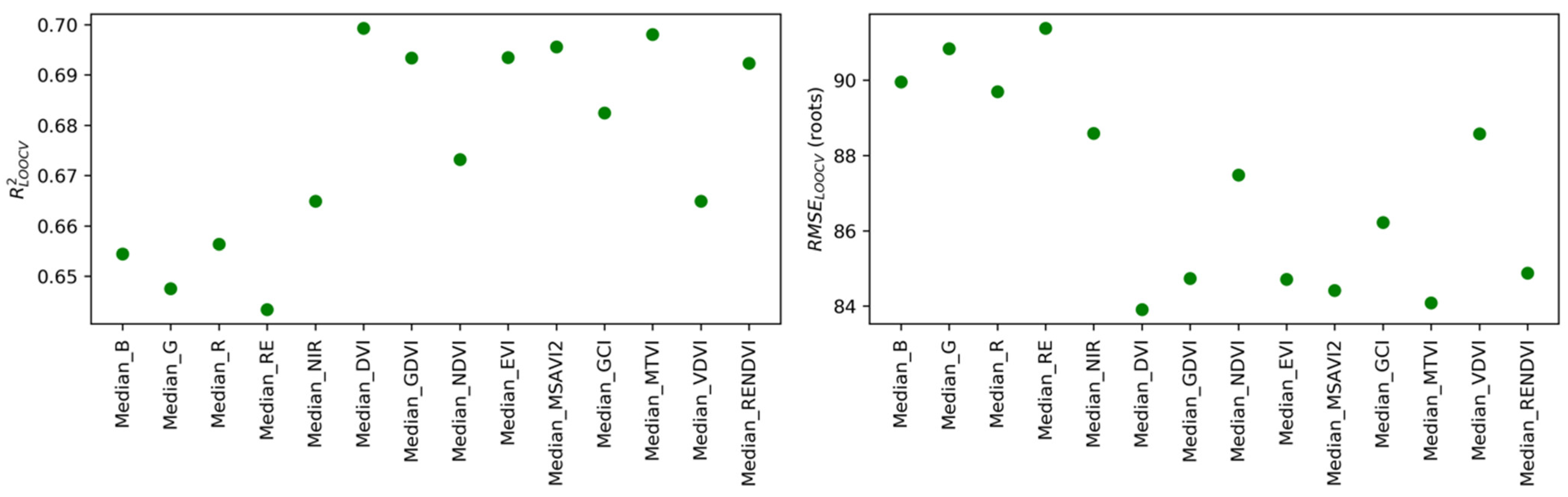
The LOOCV scores for each band and VI paired with canopy area are shown in Figure 6 for the area-augmented emergence imagery. The VIs generally outperformed the individual reflectance bands, and nearly all combinations provided an improvement to the canopy area alone ( roots). The best pair was DVI and canopy area with and roots (24% of the mean root count for all area-augmented plots). A sample of DVI + Area prediction vs. measured root counts is shown in the left panel of Figure 7 using 90% training and 10% testing data. While the radiometric features individually provided little predictive ability for the area-augmented dataset, their combination with canopy area clearly provides an improvement on area alone. The predictions for larger augmented plots are promising and distributed normally, but the predictions of the original plots are skewed to overpredicting in the majority of cases.
We further trained the DVI + Area model using the 2018 area-augmented emergence imagery and tested on the area-augmented imagery from 2019 obtained on 16 July, closest to emergence for that season. The predictions for this model are shown in the right panel of Figure 7. The model underpredicts several of the larger augmented plots with an roots or 35% of the mean root count for the 2019 area-augmented plots.
3.2. Beet Root Mass 2018
The LOOCV scores for root mass modeled with the standard plot imagery from each growth stage are compiled in Table 5. The highest R2 and lowest RMSE were found for the canopy closing imagery. However, the improvements to between growth stages were minimal. The canopy area ( kg) alone was most informative at the canopy closing growth stage while VDVI ( kg) when combined in the MLR model ( kg) provided meager improvement. The optimal of 0.9 kg is 10% of the mean root mass for all plots (or approximately 4800 kg/hectare).
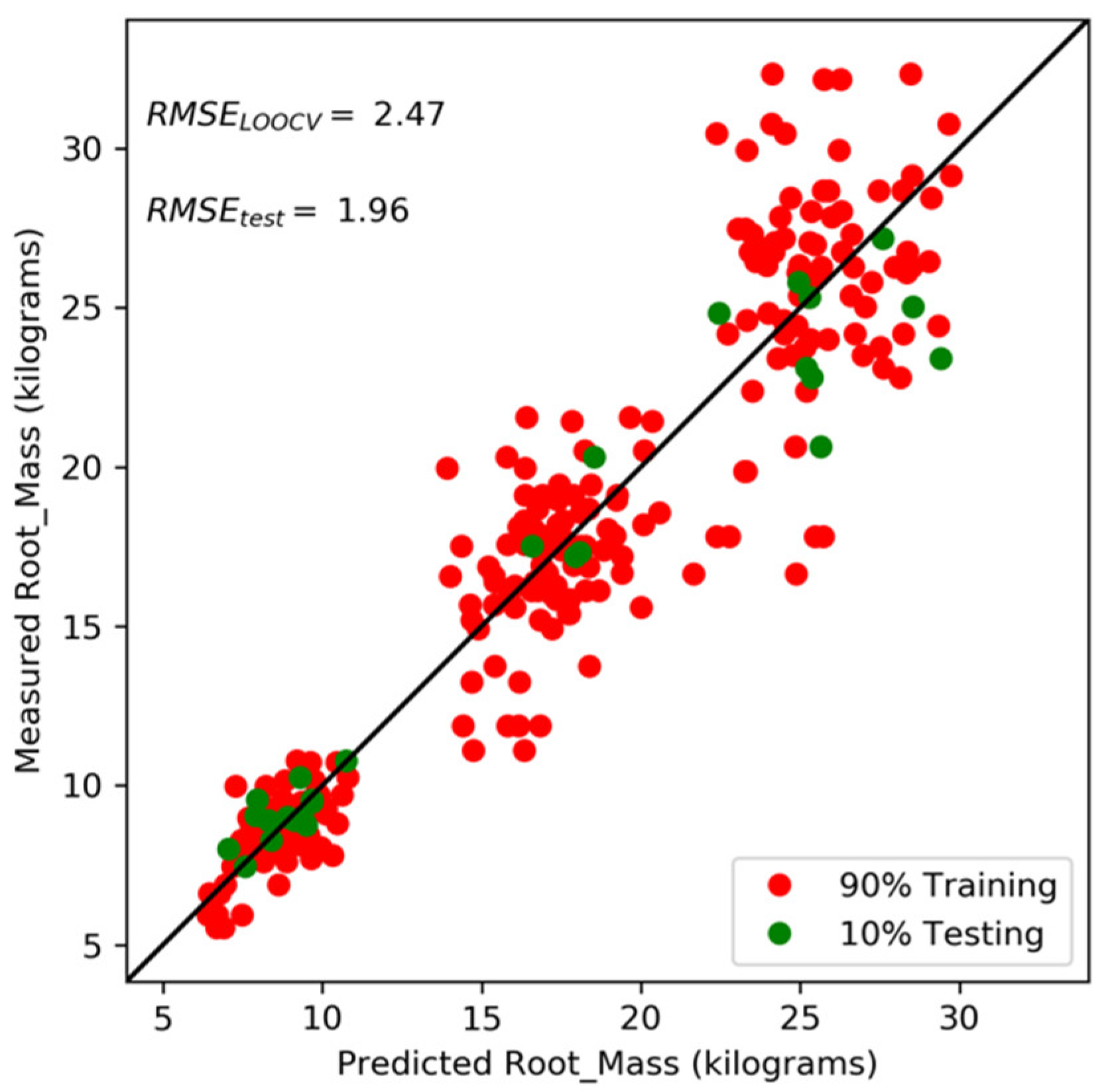
The LOOCV scores for each band and VI paired with canopy area are shown in Figure 8 for the area-augmented canopy closing imagery. The best pairing was VDVI and canopy area, but all reflectance bands and VIs offered no improvement to canopy area alone ( kg per area-augmented plot or approximately 6700 kg/hectare). The total root mass amongst the plots exhibited less variation than the root count and appear as three distinct clusters after augmentation-original plots, double combo-plots, and triple-combo plots (Figure 9). Capturing the relationship between radiometric data and root mass may require plots with a broader range of root mass.
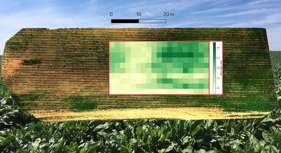
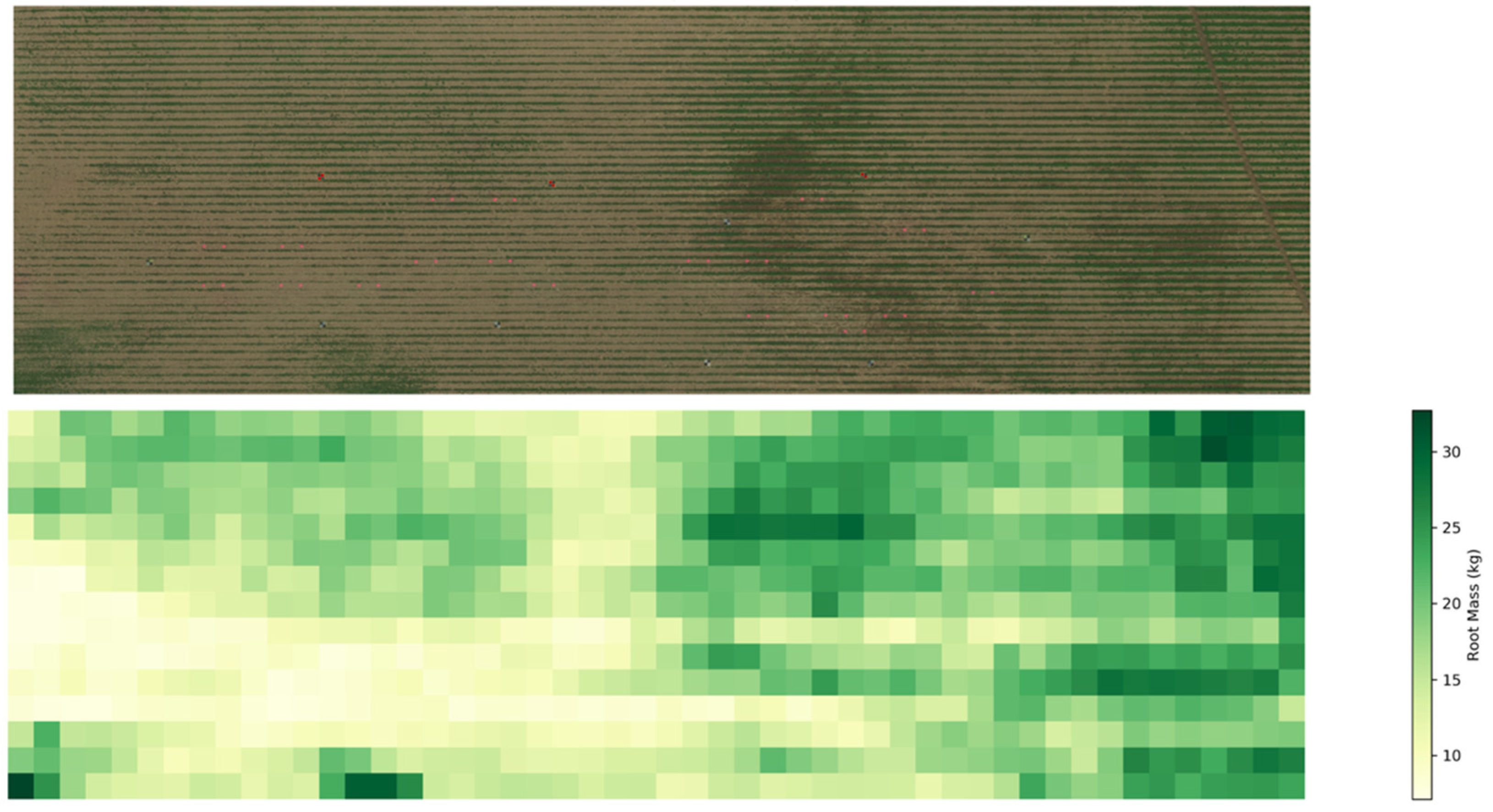
The average attainable table beet root yield in New York is estimated at 40,000 kg/hectare (J. Henderson, personal communication). We, therefore, applied our area-augmented table beet root mass model to new data for a large section (~0.3 ha) of the 2019 field imagery to assess the yield for the entire image coverage. Again, the 2019 data used here did not coincide with the exact growth stage of the 2018 canopy closing dataset used to build the area-augmented beet root mass model. Regardless, the results of our model applied to the 2019 field are shown in Figure 10. We predicted a total yield of 41,000 kg/ha, where the average grid cell (~4 m2) had table beet roots totaling kg, by tallying the root mass from each grid cell and dividing by the total area. Considering the differences in the canopy growth used to construct and test the model, this performance should merely be taken as a moderate prediction, rather than proof of concept.
3.3. Beet Root Diameter 2018
The LOOCV scores for root mass modeled with the standard plot imagery from each growth stage are compiled in Table 6. While the emergence data had the highest correlations to root diameter the correlations were lower than for root count and mass. The NIR band was most correlated with root diameter ( mm), but the canopy area ( mm) offered no improvement in the combined MLR model ( mm). The average root diameter was not explored further in this study with area-augmented imagery because the average root diameter does not scale in the same manner as table beet root count and mass.
The average root diameter exhibited poor correlation with radiometric features and the canopy area. However, when we separate the table root counts into standard diameter ranges (John Henderson, private communication), the three diameter ranges nearest the center of the diameter distribution (10–25 mm, 25–44 mm, and 44–63 mm), had the highest NIR + Area MLR model correlations (LOOCV and , respectively) with emergence plot imagery. This is expected, as they make up the largest percentages of the total root count. We show the percentage of roots falling in each of the processing diameter ranges in Figure 11, along with target percentages. The actual numbers from the test plots indicated over-production of smaller diameter and less production of larger diameter beets. Additional emergence data may be used to develop a root size distribution model in the future, but currently the low numbers for the 63–75 mm range prevent meaningful size distribution modeling in the three ranges that are key to a typical grower target.
3.4. Foliage Mass 2018
The LOOCV scores for root mass modeled with the standard plot imagery from each growth stage are compiled in Table 7. The harvest growth stage provided the best correlation with the dry weight of foliage. The combination of VIs and canopy area produced the best MLR model ( g), but neither the individual RENDVI ( g) or canopy area ( g) model had comparable performance.
The canopy area for all plots varied by the smallest margin at harvest (0.35 m2). Ultimately, all plots from 2018 reached maximum canopy area by the canopy-closed growth stage. Therefore, the canopy area loses value for predicting yield components. Moreover, any variation explained by canopy area at later growth stages is likely due to differences in pixel shading of the plots, rather than actual area. Later growth stage models should rely most heavily on the radiometric features, but these also reach a point of saturation or lack of variation between plots in most cases, as a function of closed-canopy table beets. It has been shown that typical red-near-infrared vegetation indices, such as NDVI, saturate at high Leaf Area Index (LAI) values [53]. Although we did not measure LAI explicitly, it is likely that closed canopies result in a reduction in predictive power for such red-near-infrared vegetation indices.
We did not test foliage models on the 2019 data, because we did not obtain imagery of the canopy-closed and harvest growth stages or gather the foliage mass ground truth for that year. Additionally, measured foliage mass was only modestly correlated with root mass and root count (R2 = 0.38 and 0.23, respectively). We see limited value in the development of a precise foliar biomass model without first expanding our dataset to more clearly exploit any potential relationship between foliar biomass and root yield.
4. Discussion
The performance of the 2018 area-augmented root count and mass models assessed on the 2019 data is promising, especially considering the slight differences in growth stages, in both cases. In fact, the median DVI values for the 2019 plots ranged from 0.28 to 0.49 compared to 0.20 to 0.32 in 2018, indicating that the earliest 2019 imagery captured a more advanced stage of canopy growth than the 2018 emergence data used to develop the root count model. Additionally, the smallest plots used to construct the model were twice as long as the 2019 plots. We thus recommend that additional imagery, collected on several days following emergence, could help pinpoint an optimal time to capture imagery for table beet root count predictions. Alternatively, more data may allow the use of a temporal feature representing the growth stage in our prediction model.
Similarly, there is significant potential to develop improved root mass models with additional data collected at different days during the emergence and canopy closing growth stages. Even though the Band/VI + Area root mass models did not improve upon the Area-only model, using the radiometric properties of the canopy to quantify area before closure is an effective method to predict table beet root yield.
The physical size of the canopy growth arguably should have the strongest correlation with yield, when measured close to harvest. However, by the canopy-closed growth stage observations in 2018, every plot canopy had merged with neighboring rows, thereby resulting in virtually identical canopy area. The radiometric (image) data also lacked the significant variability needed to predict a variety of root yield components for the plots by the canopy-closed growth stage. In other words, it appears that eventually the plots reach a state of maturity where they become less distinguishable in terms of vegetated area and their radiometric properties. This finding also has been demonstrated in previous studies, where especially red-NIR vegetation indices saturate and thus become less sensitive under high Leaf Area Index (LAI) or canopy-closed scenarios [53,54].
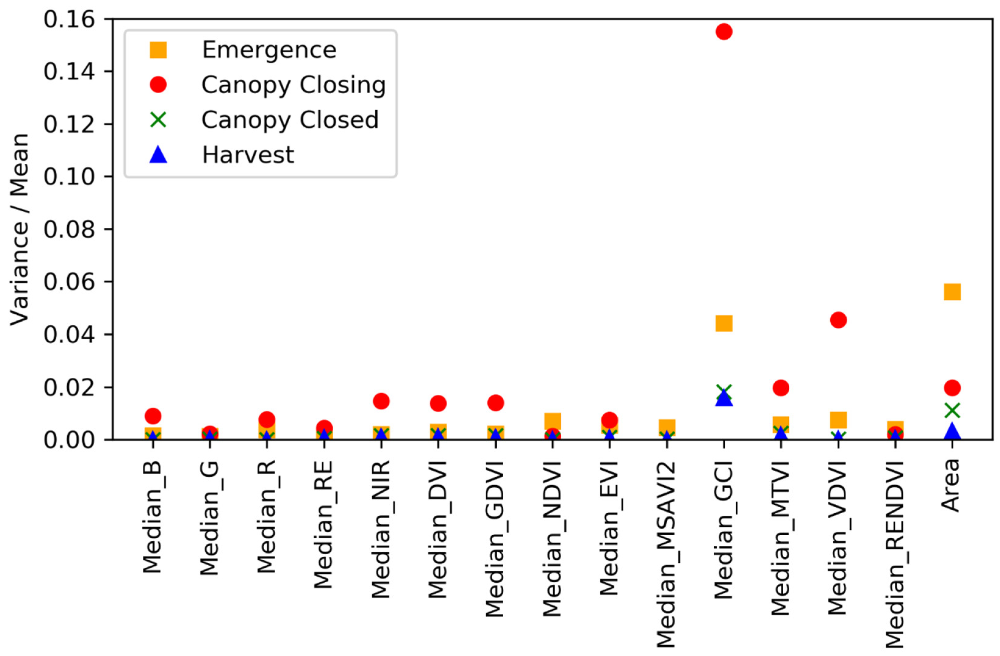
The need for early growth stage imagery is highlighted by Figure 12, where we show the radiometric variance of each input feature for the 2018 study, divided by the mean of the feature for each of the growth stages. The emergence and canopy closing growth stages exhibited the highest ratio of feature variance, normalized by the mean. Many of the radiometric features showed minimal variance (<2%) across plots. All of the canopy-closed and harvest stage radiometric features exhibited minimal variation amongst the plots. The canopy area showed the clearest trend of decreasing variation as the canopy grew into the between-row space. We, therefore, contend that monitoring the early growth stages more closely and determining when each plot reaches maturity may be more relevant to root development and ultimately, yield component prediction.
The inclusion of 3D structural features, such as canopy heights from either light detection and ranging (LiDAR) or via image-based structure-from-motion (photogrammetry) may improve predictions for future studies. We might effectively exploit the imaging data to determine both canopy area and height, supplemented with the radiometric data when it is most variable early in the season to provide early predictions. Even if the canopy area and vegetation indices have reached saturation, canopy height may continue to exhibit variability between plots at the later growth stages and provide a more direct measure of the foliar biomass.
In addition to acquiring imagery more frequently, ground truth data should be obtained from a larger sample size. A larger number of smaller scale samples covering an identical area could be accomplished with equivalent sampling labor to reach a higher base sample size. The area-augmented procedure used here could then be applied to model scalable yield components. A future study may also use hyperspectral data derived from an UAS or handheld spectrometer, with the goal of determining a set of spectral bands that exhibit optimal association with yield components [55], thereby improving upon the multispectral bands used in this study.
Plots with obvious visual evidence of weeds were removed as outliers before regression modeling. We, therefore, would need to incorporate a method for identifying and mapping weeds between rows in the early growth stages, as implemented by Pérez-Ortiz et al. [56] for sunflower crops, if we were to apply our models to a table beet field. An early, targeted elimination of weeds in problem areas may prevent the low root yields that we observed in four test plots that contained obvious examples of weed growth between rows in the emergence 2018 imagery (i.e., plots 41–43 and 46; Figure 2).
5. Conclusions
We evaluated the use of five-band visible-near-infrared UAS imagery to assess New York table beet root yield (root count and mass) across four airborne campaigns spanning the 2018 cropping season. Overall, our investigations of table beet root yield uncovered the need to obtain additional data, at different times throughout the early growth stages, and to prioritize flight plans for also obtaining canopy heights from our imagery using structure-from-motion (photogrammetry) or LiDAR data. We observed modest predictive ability for both the root count ( roots) and root mass models ( kg) using UAS multispectral imagery. However, extending 2018 single-year models to independent data, e.g., full 2019 field or 2019 plot-level imagery, was successful after incorporating area-augmented plots (vegetation coverage/plot). These models took advantage of the obvious relationship between canopy area and root yield/count.
In reality, any application of a crop yield model based on radiometric information from satellites, UAS, or over-the-row tractor equipment needs to be robust to a multitude of scales and conditions. A model developed solely from radiometric data of a standard plot size likely will not be ideal if the goal is to apply these results in the field. Our area-augmented modeling demonstrates potential to create a model robust to this shortcoming by using a combination of radiometric and spatial (coverage or structural) data. We thus recommend that more data from an array of growth stages and seasons be included in future studies to develop more confidence in the operational UAS-based yield modeling applications.
Author Contributions
Conceptualization, R.C., J.v.A., S.P., D.C. and J.H.; data curation, R.C. and J.v.A.; formal analysis, R.C. and J.v.A.; funding acquisition, J.v.A., S.P., D.C. and J.H.; investigation, R.C. and J.v.A.; methodology, R.C. and J.v.A.; project administration, J.v.A.; resources, S.P., D.C. and J.H.; supervision, J.v.A.; validation, R.C. and J.v.A.; visualization, R.C.; writing—original draft, R.C.; writing—review and editing, J.v.A., S.P., D.C. and J.H. All authors have read and agreed to the published version of the manuscript.
Funding
This research was supported by Love Beets USA, and the United States Department of Agriculture, National Institute of Food and Agriculture Health project NYG-625424, managed by Cornell AgriTech at the New York State Agricultural Experiment Station (NYSAES), Cornell University, Geneva, New York. R.C. and J.v.A. were supported by National Science Foundation, Partnerships for Innovation Award No. 1827551.
Institutional Review Board Statement
Not applicable.
Informed Consent Statement
Not applicable.
Data Availability Statement
Not applicable.
Acknowledgments
We credit Tim Bauch and Nina Raqueno of the RIT drone team who were responsible for capturing the UAS imagery used for this study, with the direction of Ethan Hughes and Jan van Aardt. Thanks also to Carol Bowden and Sean Murphy, Cornell AgriTech, for assistance with collecting agronomic data, and growers for access to their fields. We would also like to thank Love Beets USA for sharing standard production information for the New York table beet industry.
Conflicts of Interest
The authors declare no conflict of interest.
References
- USDA. National Agricultural Statistics Service 2012 Census of Agriculture; USDA: Washington, DC, USA, 2014.
- Clifford, T.; Howatson, G.; West, D.J.; Stevenson, E.J. The Potential Benefits of Red Beetroot Supplementation in Health and Disease. Nutrients 2015, 7, 2801–2822. [Google Scholar] [CrossRef]
- Gilchrist, M.; Winyard, P.G.; Fulford, J.; Anning, C.; Shore, A.C.; Benjamin, N. Dietary Nitrate Supplementation Improves Reaction Time in Type 2 Diabetes: Development and Application of a Novel Nitrate-Depleted Beetroot Juice Placebo. Nitric Oxide Biol. Chem. 2014, 40, 67–74. [Google Scholar] [CrossRef]
- Hobbs, D.A.; Kaffa, N.; George, T.W.; Methven, L.; Lovegrove, J.A. Blood Pressure-Lowering Effects of Beetroot Juice and Novel Beetroot-Enriched Bread Products in Normotensive Male Subjects. Br. J. Nutr. 2012, 108, 2066–2074. [Google Scholar] [CrossRef] [Green Version]
- Georgiev, V.G.; Weber, J.; Kneschke, E.M.; Denev, P.N.; Bley, T.; Pavlov, A.I. Antioxidant Activity and Phenolic Content of Betalain Extracts from Intact Plants and Hairy Root Cultures of the Red Beetroot Beta Vulgaris cv. Detroit Dark Red. Plant Foods Hum. Nutr. 2010, 65, 105–111. [Google Scholar] [CrossRef] [PubMed]
- Vanhatalo, A.; Bailey, S.J.; Blackwell, J.R.; DiMenna, F.J.; Pavey, T.G.; Wilkerson, D.P.; Benjamin, N.; Winyard, P.G.; Jones, A.M. Acute and Chronic Effects of Dietary Nitrate Supplementation on Blood Pressure and the Physiological Responses to Moderate-Intensity and Incremental Exercise. Am. J. Physiol. Regul. Integr. Comp. Physiol. 2010, 299, 1121–1131. [Google Scholar] [CrossRef] [PubMed] [Green Version]
- Szalaty, M. Physiological Roles and Availability of Betacyanins. Adv. Phytother. 2008, 1, 20–25. [Google Scholar]
- Weiss, M.; Jacob, F.; Duveiller, G. Remote Sensing for Agricultural Applications: A Meta-Review. Remote Sens. Environ. 2020. [Google Scholar] [CrossRef]
- Mulla, D.J. Twenty Five Years of Remote Sensing in Precision Agriculture: Key Advances and Remaining Knowledge Gaps. Biosyst. Eng. 2013, 114, 358–371. [Google Scholar] [CrossRef]
- Pierpaoli, E.; Carli, G.; Pignatti, E.; Canavari, M. Drivers of Precision Agriculture Technologies Adoption: A Literature Review. Procedia Technol. 2013, 8, 61–69. [Google Scholar] [CrossRef] [Green Version]
- Atzberger, C. Advances in Remote Sensing of Agriculture: Context Description, Existing Operational Monitoring Systems and Major Information Needs. Remote Sens. 2013, 5, 949–981. [Google Scholar] [CrossRef] [Green Version]
- Schimmelpfennig, D. Farm Profits and Adoption of Precision Agriculture; USDA: Washington, DC, USA, 2016.
- Stroppiana, D.; Migliazzi, M.; Chiarabini, V.; Crema, A.; Musanti, M.; Franchino, C.; Villa, P. Rice Yield Estimation Using Multispectral Data from UAV: A Preliminary Experiment in Northern Italy. In Proceedings of the 2015 IEEE International Geoscience and Remote Sensing Symposium (IGARSS), Milan, Italy, 26–31 July 2015; pp. 4664–4667. [Google Scholar]
- Duan, B.; Fang, S.; Zhu, R.; Wu, X.; Wang, S.; Gong, Y.; Peng, Y. Remote Estimation of Rice Yield with Unmanned Aerial Vehicle (UAV) Data and Spectral Mixture Analysis. Front. Plant Sci. 2019, 10, 204. [Google Scholar] [CrossRef] [PubMed] [Green Version]
- Maresma, Á.; Lloveras, J.; Martinez-Casasnovas, J.A. Use of Multispectral Airborne Images to Improve In-Season Nitrogen Management, Predict Grain Yield and Estimate Economic Return of Maize in Irrigated High Yielding Environments. Remote Sens. 2018, 10, 543. [Google Scholar] [CrossRef] [Green Version]
- Barzin, R.; Pathak, R.; Lotfi, H.; Varco, J.; Bora, G.C. Use of UAS Multispectral Imagery at Different Physiological Stages for Yield Prediction and Input Resource Optimization in Corn. Remote Sens. 2020, 12, 2392. [Google Scholar] [CrossRef]
- Hassan, M.A.; Yang, M.; Rasheed, A.; Yang, G.; Reynolds, M.; Xia, X.; Xiao, Y.; He, Z. A Rapid Monitoring of NDVI across the Wheat Growth Cycle for Grain Yield Prediction Using a Multi-Spectral UAV Platform. Plant Sci. 2019, 282, 95–103. [Google Scholar] [CrossRef] [PubMed]
- Zhou, X.; Zheng, H.B.; Xu, X.Q.; He, J.Y.; Ge, X.K.; Yao, X.; Cheng, T.; Zhu, Y.; Cao, W.X.; Tian, Y.C. Predicting Grain Yield in Rice Using Multi-Temporal Vegetation Indices from UAV-Based Multispectral and Digital Imagery. ISPRS J. Photogramm. Remote Sens. 2017, 130, 246–255. [Google Scholar] [CrossRef]
- Olson, D.; Chatterjee, A.; Franzen, D.W.; Day, S.S. Relationship of Drone-Based Vegetation Indices with Corn and Sugarbeet Yields. Agron. J. 2019, 111, 2545–2557. [Google Scholar] [CrossRef]
- Olson, D.; Chatterjee, A.; Franzen, D.W. Can We Select Sugarbeet Harvesting Dates Using Drone-based Vegetation Indices? Agron. J. 2019, 111, 2619–2624. [Google Scholar] [CrossRef]
- Bu, H.; Sharma, L.K.; Denton, A.; Franzen, D.W. Comparison of Satellite Imagery and Ground-Based Active Optical Sensors as Yield Predictors in Sugar Beet, Spring Wheat, Corn, and Sunflower. Agron. J. 2017, 109, 299–308. [Google Scholar] [CrossRef] [Green Version]
- Wanjura, D.F.; Hudspeth, E.B.; Bilbro, J.D. Emergence Time, Seed Quality, and Planting Depth Effects on Yield and Survival of Cotton (Gossypium hirsutum L.). Agron. J. 1969, 61, 63–65. [Google Scholar] [CrossRef]
- Virk, G.; Pilon, C.; Snider, J.L. Impact of First True Leaf Photosynthetic Efficiency on Peanut Plant Growth under Different Early-Season Temperature Conditions. Peanut Sci. 2019, 46, 162–173. [Google Scholar] [CrossRef]
- Raun, W.R.; Solie, J.B.; Johnson, G.V.; Stone, M.L.; Lukina, E.V.; Thomason, W.E.; Schepers, J.S. In-Season Prediction of Potential Grain Yield in Winter Wheat Using Canopy Reflectance. Agron. J. 2001, 93, 131–138. [Google Scholar] [CrossRef] [Green Version]
- Al-Gaadi, K.A.; Hassaballa, A.A.; Tola, E.; Kayad, A.G.; Madugundu, R.; Alblewi, B.; Assiri, F. Prediction of Potato Crop Yield Using Precision Agriculture Techniques. PLoS ONE 2016, 11, e0162219. [Google Scholar] [CrossRef]
- MicaSense RedEdge-M User Manual. Available online: https://support.micasense.com/hc/en-us/articles/115003537673-RedEdge-M-User-Manual-PDF- (accessed on 11 March 2021).
- Pix4D Pix4D Mapper. Available online: https://www.pix4d.com/product/pix4dmapper-photogrammetry-software (accessed on 11 March 2021).
- Mamaghani, B.; Salvaggio, C. Multispectral Sensor Calibration and Characterization for SUAS Remote Sensing. Sensors 2019, 19, 4453. [Google Scholar] [CrossRef] [Green Version]
- Pix4Dmapper Support: Radiometric Corrections. Available online: https://support.pix4d.com/hc/en-us/articles/202559509-Radiometric-corrections (accessed on 18 May 2021).
- MicaSense DLS 2 Integration Guide. Available online: https://support.micasense.com/hc/en-us/articles/360011569434-DLS-2-Integration-Guide (accessed on 18 May 2021).
- L3Harris ENVI. Available online: https://www.l3harrisgeospatial.com/Software-Technology/ENVI (accessed on 11 March 2021).
- Photonics, H. Hyperspectral Software Headwall Photonics Software. Available online: https://www.headwallphotonics.com/software (accessed on 19 May 2021).
- Using ENVI: Atmospheric Correction—Empirical Line Correction. Available online: https://www.l3harrisgeospatial.com/docs/atmosphericcorrection.html#empirical_line_calibration (accessed on 24 May 2021).
- Boggs, T. Spectral Python (SPy). Available online: http://www.spectralpython.net/ (accessed on 11 March 2021).
- Oshigami, S.; Yamaguchi, Y.; Uezato, T.; Momose, A.; Arvelyna, Y.; Kawakami, Y.; Yajima, T.; Miyatake, S.; Nguno, A. Mineralogical Mapping of Southern Namibia by Application of Continuum-Removal MSAM Method to the HyMap Data. Int. J. Remote Sens. 2013, 34, 5282–5295. [Google Scholar] [CrossRef]
- Tichy, L.; Chutry, M.; Botta-Dukát, Z. Semi-Supervised Classification of Vegetation: Preserving the Good Old Units and Searching for New Ones. J. Veg. Sci. 2014, 25, 1504–1512. [Google Scholar] [CrossRef] [Green Version]
- Sader, S.A.; Winne, J.C. RGB-NDVI Colour Composites for Visualizing Forest Change Dynamics. Int. J. Remote Sens. 1992, 13, 3055–3067. [Google Scholar] [CrossRef]
- Gallo, B.C.; Demattê, J.A.M.; Rizzo, R.; Safanelli, J.L.; de Mendes, W.S.; Lepsch, I.F.; Sato, M.V.; Romero, D.J.; Lacerda, M.P.C. Multi-Temporal Satellite Images on Topsoil Attribute Quantification and the Relationship with Soil Classes and Geology. Remote Sens. 2018, 10, 1571. [Google Scholar] [CrossRef]
- Broge, N.H.; Leblanc, E. Comparing Prediction Power and Stability of Broadband and Hyperspectral Vegetation Indices for Estimation of Green Leaf Area Index and Canopy Chlorophyll Density. Remote Sens. Environ. 2001, 76, 156–172. [Google Scholar] [CrossRef]
- Gitelson, A.A.; Merzlyak, M.N.; Lichtenthaler, H.K. Detection of Red Edge Position and Chlorophyll Content by Reflectance Measurements near 700 Nm. J. Plant Physiol. 1996, 148, 501–508. [Google Scholar] [CrossRef]
- Trunk, G.V. A Problem of Dimensionality: A Simple Example. IEEE Trans. Pattern Anal. Mach. Intell. 1979, 3, 306–307. [Google Scholar] [CrossRef] [PubMed]
- Tucker, C.J. Red and Photographic Infrared Linear Combinations for Monitoring Vegetation. Remote Sens. Environ. 1979, 8, 127–150. [Google Scholar] [CrossRef] [Green Version]
- Sripada, R.P. Determining in-Season Nitrogen Requirements for Corn Using Aerial Color-Infrared Photography. Ph.D. Thesis, North Carolina State University, Raleigh, NC, USA, 2005. [Google Scholar]
- Gamon, J.A.; Field, C.B.; Goulden, M.L.; Griffin, K.L.; Hartley, A.E.; Joel, G.; Peñuelas, J.; Valentini, R. Relationships between NDVI, Canopy Structure, and Photosynthesis in Three Californian Vegetation Types. Ecol. Appl. 1995, 5, 28–41. [Google Scholar] [CrossRef] [Green Version]
- Huete, A.; Didan, K.; Miura, T.; Rodriguez, E.P.; Gao, X.; Ferreira, L.G. Overview of the Radiometric and Biophysical Performance of the MODIS Vegetation Indices. Remote Sens. Environ. 2002, 83, 195–213. [Google Scholar] [CrossRef]
- Qi, J.; Chehbouni, A.; Huete, A.R.; Kerr, Y.H.; Sorooshian, S. A Modified Soil Adjusted Vegetation Index. Remote Sens. Environ. 1994, 48, 119–126. [Google Scholar] [CrossRef]
- Gitelson, A.A.; Gritz, Y.; Merzlyak, M.N. Relationships between Leaf Chlorophyll Content and Spectral Reflectance and Algorithms for Non-Destructive Chlorophyll Assessment in Higher Plant Leaves. J. Plant Physiol. 2003, 160, 271–282. [Google Scholar] [CrossRef]
- Haboudane, D.; Miller, J.R.; Pattey, E.; Zarco-Tejada, P.J.; Strachan, I.B. Hyperspectral Vegetation Indices and Novel Algorithms for Predicting Green LAI of Crop Canopies: Modeling and Validation in the Context of Precision Agriculture. Remote Sens. Environ. 2004, 90, 337–352. [Google Scholar] [CrossRef]
- Xiaoqin, W.; Miaomiao, W.; Shaoqiang, W.; Yundong, W. Extraction of Vegetation Information from Visible Unmanned Aerial Vehicle Images. Trans. Chin. Soc. Agric. Eng. 2015, 31, 152–159. [Google Scholar]
- Sims, D.A.; Gamon, J.A. Relationships between Leaf Pigment Content and Spectral Reflectance across a Wide Range of Species, Leaf Structures and Developmental Stages. Remote Sens. Environ. 2002, 81, 337–354. [Google Scholar] [CrossRef]
- Louhaichi, M.; Borman, M.M.; Johnson, D.E. Spatially Located Platform and Aerial Photography for Documentation of Grazing Impacts on Wheat. Geocarto Int. 2001, 16, 65–70. [Google Scholar] [CrossRef]
- Afifi, A.; May, S.; Donatello, R.; Clark, V. Practical Multivariate Analysis, 6th ed.; CRC Press: New York, NY, USA, 2019. [Google Scholar]
- Gu, Y.; Wylie, B.K.; Howard, D.M.; Phuyal, K.P.; Ji, L. NDVI Saturation Adjustment: A New Approach for Improving Cropland Performance Estimates in the Greater Platte River Basin, USA. Ecol. Indic. 2013, 30, 1–6. [Google Scholar] [CrossRef]
- Prabhakara, K.; Hively, W.D.; McCarty, G.W. Evaluating the Relationship between Biomass, Percent Groundcover and Remote Sensing Indices across Six Winter Cover Crop Fields in Maryland, United States. Int. J. Appl. Earth Obs. Geoinf. 2015, 39, 88–102. [Google Scholar] [CrossRef] [Green Version]
- Hassanzadeh, A.; van Aardt, J.; Murphy, S.P.; Pethybridge, S.J. Yield Modeling of Snap Bean Based on Hyperspectral Sensing: A Greenhouse Study. JARS 2020, 14, 024519. [Google Scholar] [CrossRef]
- Pérez-Ortiz, M.; Peña, J.M.; Gutiérrez, P.A.; Torres-Sánchez, J.; Hervás-Martinez, C.; López-Granados, F. A Semi-Supervised System for Weed Mapping in Sunflower Crops Using Unmanned Aerial Vehicles and a Crop Row Detection Method. Appl. Soft Comput. 2015, 37, 533–544. [Google Scholar] [CrossRef]
Figure 1.
The 2018 and 2019 table beet field site locations in Batavia, New York, USA. Lower left map data: Google, Maxar Technologies.
Figure 1.
The 2018 and 2019 table beet field site locations in Batavia, New York, USA. Lower left map data: Google, Maxar Technologies.

Figure 2.
RGB (color) bands of MicaSense plot imagery from 9 July 2018 at 11:00. Note the broad range in crop emergence at this early season observation. Each plot is 3 × 0.6 m in dimension and has a 0.02 m ground sampling distance.
Figure 2.
RGB (color) bands of MicaSense plot imagery from 9 July 2018 at 11:00. Note the broad range in crop emergence at this early season observation. Each plot is 3 × 0.6 m in dimension and has a 0.02 m ground sampling distance.

Figure 3.
(Left) Median blue, green, red, red edge, and near-infrared reflectance of each plot’s canopy pixels (background soil masked out) from table beet plots in New York in 2018. The vertical dashed lines separate the data in terms of the growth epochs observed in the 2018 season. (Right) The average and standard deviation of all individual plot median reflectance measurements are shown alongside the range of the individual measurements (X’s).

Figure 4.
Table beet vegetation classification for four observations of the 2018 plot # 17 using TVI > 7.5 threshold, k-means (two clusters), vegetation-endmember (average of all plot vegetation spectra) SAM > 0.85 threshold (normalized between 0 and 1, where 1 corresponds to a perfect match), and NDVI > 0.5 threshold. The binary vegetation classification masks display vegetation pixels as white and the background soil and shadow as black.

Figure 5.
Grayscale multispectral bands and vegetation indices for imagery collected in a table beet field on 16 July 2019 (example plot 16) in Batavia, New York.
Figure 5.
Grayscale multispectral bands and vegetation indices for imagery collected in a table beet field on 16 July 2019 (example plot 16) in Batavia, New York.

Figure 6.
The area-augmented table beet root count (left) and (right) leave-one-out cross-validation performance (y-axis) for individual multiple linear regression models. Each model consists of one reflectance band or vegetation index shown on the x-axis combined with canopy area. The DVI paired with table beet canopy area was the best-performing model with and roots.

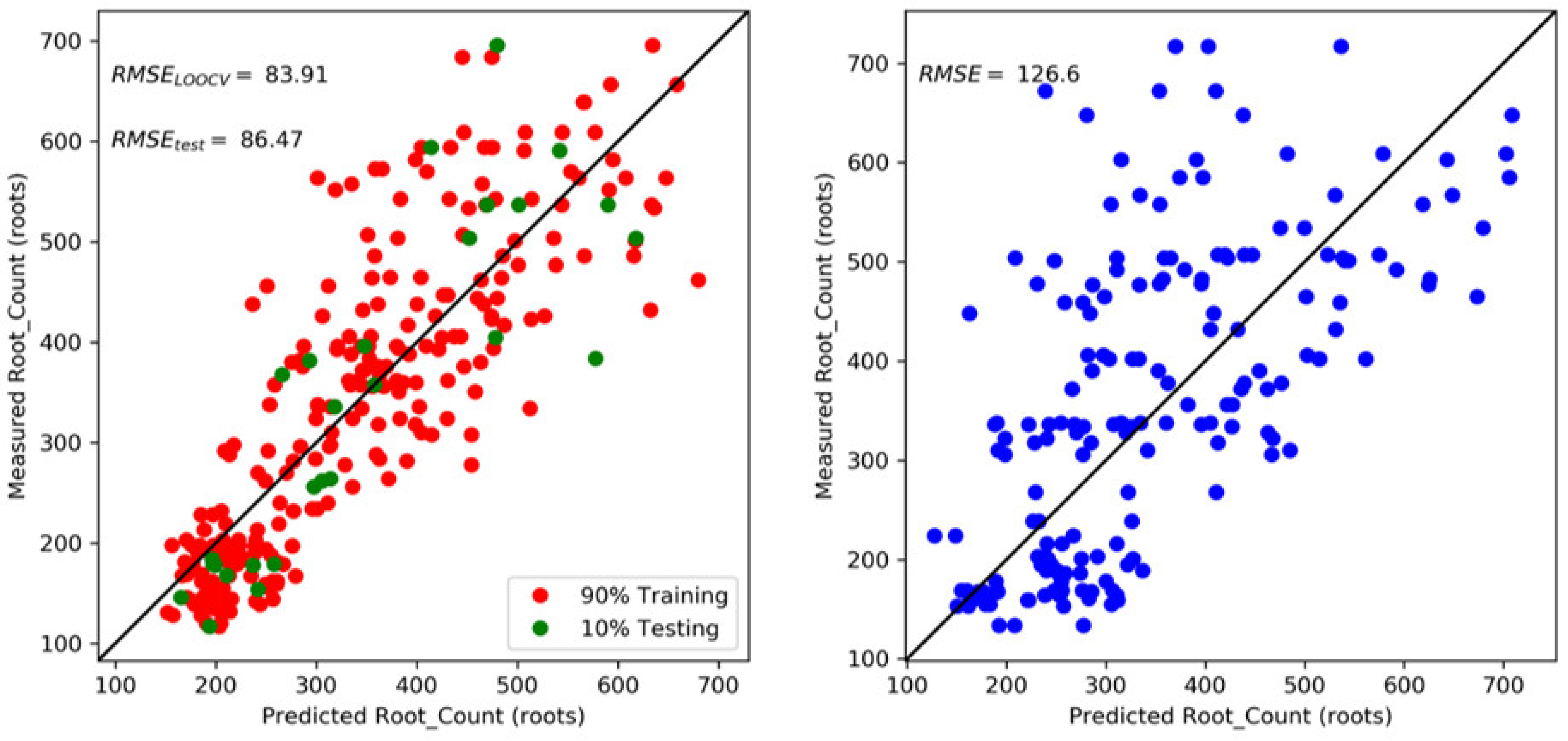
Figure 7.
Measured vs. predicted table beet root count for the 2018 emergence DVI + Area multiple linear regression model, based on area-augmented imagery (left). The model is trained with 90% (red) and tested with the remaining 10% (green) area augmented study plot imagery. RMSE are displayed for the training data using leave-one-out cross-validation and for the unseen test data. The DVI + Area model is trained with 100% of the 2018 emergence imagery and tested to predict the root count (blue) for 100% of the 2019 area-augmented study plot imagery occurring closest to emergence (right).

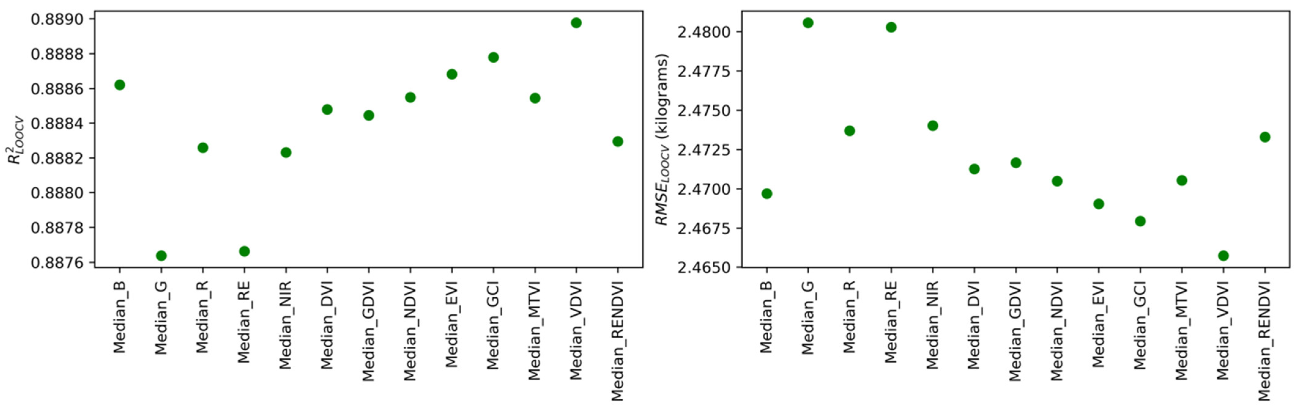
Figure 8.
The area-augmented table beet root mass (left) and (right) leave-one-out cross-validation performance (y-axis) for individual multiple linear regression models. Each model consists of one reflectance band or vegetation index shown on the x-axis combined with canopy area. The VDVI paired with canopy area was the best-performing model with and kg. However, the vertical axis scaling shown for both plots indicates that the radiometric data provide no significant improvement to the table beet root mass model derived from the area-augmented imagery.

Figure 9.
Measured vs. predicted table beet root mass for the 2018 canopy closing VDVI + Area multiple linear regression model based on area-augmented plot imagery. The model is trained with 90% (red) and tested with the remaining 10% (green) area-augmented study plot imagery. RMSE are displayed for the training data using leave-one-out cross-validation and for the unseen test data.

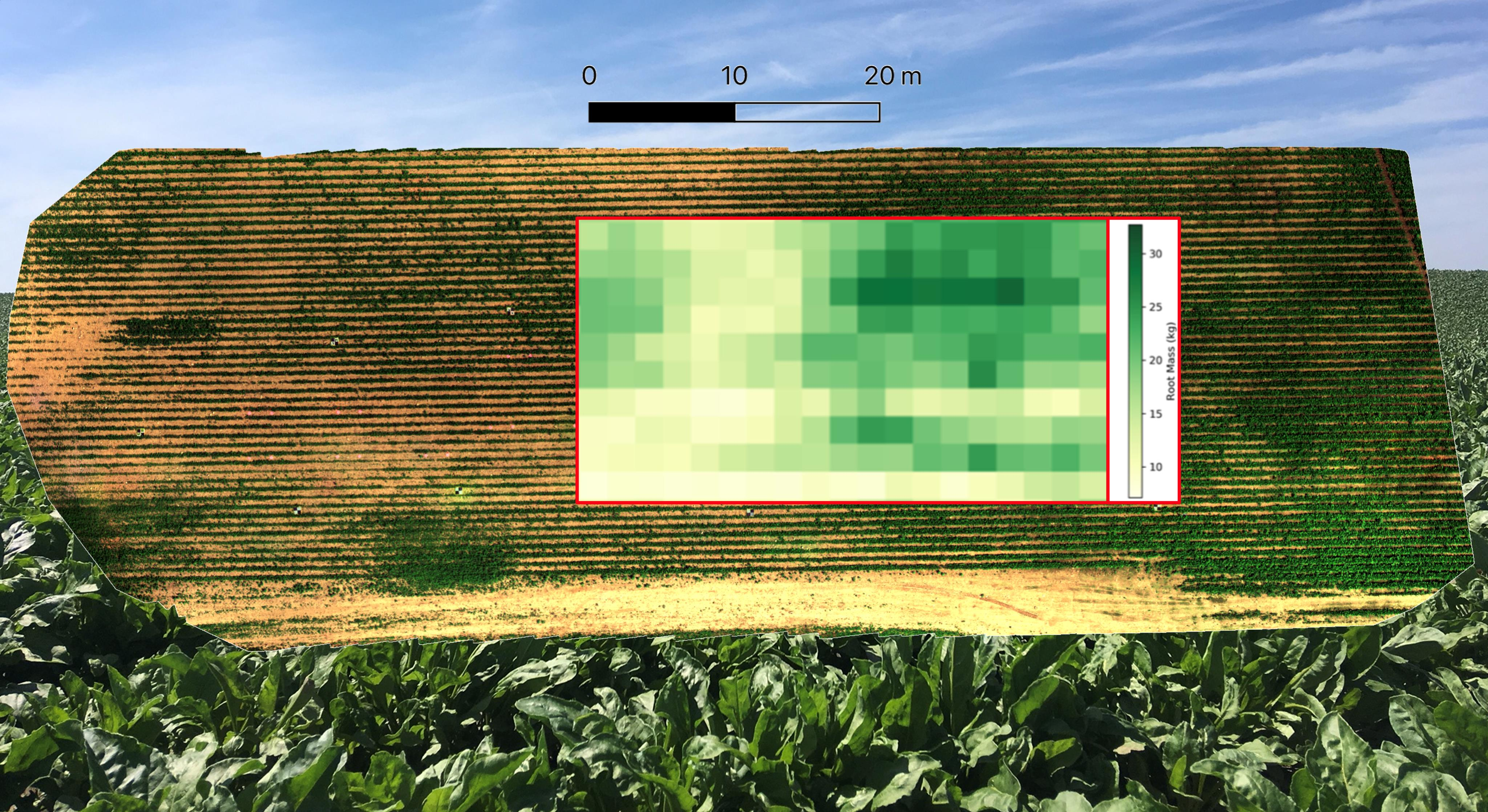
Figure 10.
An evaluation of the area-augmented 2018 table beet root mass model on the independent augmented area plot imagery, taken on 16 July 2019. Since we do not have ground truth root mass data for the 2019 plots, we applied the model to the whole field for an approximate assessment. An RGB composite (top) of a large portion of the 2019 field serves as context for the 2 × 2 m grid of the field with the table beet root mass model.

Figure 11.
The median percentage of all 2018 plots’ table beet roots, falling in each diameter range, are plotted in green inside of a box spanning the inter quantile range (IQR). Outliers are marked with black open circles and fall outside the error bars located at Quantile 3 + 1.5 IQR (above) and Quantile 1–1.5 IQR (below). The optimal percentages of table beet roots falling in each range, as provided by Love Beets USA (a commercial beet grower), is plotted with red filled circles.

Figure 12.
There was limited radiometric variability for each New York table beet growth stage in 2018. The cumulative experimental plot variance is divided by the mean of each radiometric feature and canopy area. The emergence and canopy closing growth stages exhibited the most variable features amongst the full set of plots, reinforcing the modeling results.


Table 1.
Temporal sequence of data collection in the table beet fields in New York, USA in 2018 and 2019.
Table 1.
Temporal sequence of data collection in the table beet fields in New York, USA in 2018 and 2019.
| Year/Assessment | Ground Truth | UAS Canopy Reflectance | Altitude 1 (m) | GSD 2 (cm) |
|---|---|---|---|---|
| 2018: | ||||
| 1—Emergence | Stand Count (July 5) | 2 Multispectral (July 9) | 14, 27 | 1, 2 |
| 2—Canopy Closing | Stand Count (July 20–22) | 2 Hyperspectral (July 27) | 57, 49 | 3.5, 2.5 |
| 3—Canopy Closed | Stand Count (August 6) | 2 Multispectral (August 9) | 22, 35 | 1.5, 2.5 |
| 4—Harvest | Stand Count (August 20) and Yield Data (August 24) | 2 Multispectral (August 24) | 30, 45 | 2, 3 |
| 2019: | ||||
| 1—Emergence | Stand Count (July 15) | 3 Multispectral (July 16) | 14, 12, 7 | 1, 0.75, 0.5 |
| 2—Canopy Closing | Stand Count (July 24) | 3 Multispectral (July 24) | 14, 12, 7 | 1, 0.75, 0.5 |
| 3—Harvest | Stand Count (August 16) | None | ||
1 Altitude for individual flights. 2 Ground sample distance (GSD) for individual flights.
Table 2.
MicaSense RedEdge-M camera spectral bands used for quantifying reflectance from table beet canopies in New York, USA, 2018 and 2019.
Table 2.
MicaSense RedEdge-M camera spectral bands used for quantifying reflectance from table beet canopies in New York, USA, 2018 and 2019.
| Band Name | Center Wavelength (nm) | Bandwidth FWHM 1 (nm) |
|---|---|---|
| Blue | 475 | 20 |
| Green | 560 | 20 |
| Red | 668 | 10 |
| Red Edge | 717 | 10 |
| Near Infrared | 840 | 40 |
1 Full width at half maximum—FWHM.
Table 3.
Select vegetation indices used in this study.
| Index | Name | Formula |
|---|---|---|
| DVI | Difference Vegetation Index [42] | |
| GDVI | Green Difference Vegetation Index [43] | |
| NDVI | Normalized Difference Vegetation Index [44] | |
| EVI | Enhanced Vegetation Index [45] | |
| MSAVI2 | Modified Soil Adjusted Vegetation Index 2 [46] | |
| GCI | Green Chlorophyll Index [47] | |
| MTVI | Modified Triangular Vegetation Index [48] | |
| VDVI | Visible-Band Difference Vegetation Index [51] | |
| RENDVI | Red Edge Normalized Difference Vegetation Index [50] |
Table 4.
Table beet root count growth stage and band/VI assessment report with leave-one-out cross-validation R2 and root mean squared error (RMSE) for the best pairing of a radiometric feature with canopy area MLR model and the linear regression scores of the individual features in 2018.
Table 4.
Table beet root count growth stage and band/VI assessment report with leave-one-out cross-validation R2 and root mean squared error (RMSE) for the best pairing of a radiometric feature with canopy area MLR model and the linear regression scores of the individual features in 2018.
| Band/VI + Area | Area | Band/VI | |||||
|---|---|---|---|---|---|---|---|
| Growth Stage | Best Band/VI | (Roots) | (Roots) | (Roots) | |||
| Emergence | NIR | 0.38 | 22 | 0.23 | 25 | 0.4 | 22 |
| Closing | NIR | 0.03 | 28 | −0.04 | 29 | 0.04 | 28 |
| Closed | VDVI | 0.11 | 27 | −0.02 | 29 | 0.11 | 27 |
| Harvest | NIR | 0.26 | 24 | 0.23 | 25 | 0.14 | 26 |
Table 5.
Table beet root mass growth stage and band/VI assessment report with leave-one-out cross-validation R2 and root mean squared error (RMSE) for the best pairing of a radiometric feature with canopy area MLR model and the linear regression scores of the individual features in New York in 2018.
| Band/VI + Area | Area | Band/VI | |||||
|---|---|---|---|---|---|---|---|
| Growth Stage | Best Band/VI | (kg) | (Roots) | (Roots) | |||
| Emergence | RE | 0.20 | 1.0 | 0.16 | 1.1 | −0.01 | 1.2 |
| Closing | VDVI | 0.37 | 0.9 | 0.36 | 0.9 | −0.03 | 1.2 |
| Closed | MSAVI2 | 0.22 | 1.0 | 0.0 | 1.1 | 0.24 | 1.0 |
| Harvest | R | 0.18 | 1.0 | −0.01 | 1.2 | 0.11 | 1.1 |
Table 6.
Table beet root diameter growth stage and band/VI assessment report with leave-one-out cross-validation R2 and root mean squared error (RMSE) for the best pairing of a radiometric feature with canopy area MLR model and the linear regression scores of the individual features in New York in 2018.
| Band/VI + Area | Area | Band/VI | |||||
|---|---|---|---|---|---|---|---|
| Growth Stage | Best Band/VI | (mm) | (mm) | (mm) | |||
| Emergence | NIR | 0.22 | 3.2 | 0.02 | 3.5 | 0.22 | 3.2 |
| Closing | NIR | 0.08 | 3.4 | 0.0 | 3.6 | −0.01 | 3.6 |
| Closed | VDVI | −0.04 | 3.6 | −0.05 | 3.7 | −0.01 | 3.6 |
| Harvest | R | 0.18 | 3.2 | 0.14 | 3.3 | 0.08 | 3.4 |
Table 7.
Table beet growth stage and band/VI assessment report with leave-one-out cross-validation R2 and root mean squared error (RMSE) for the best pairing of a radiometric feature with canopy area MLR model and the linear regression scores of the individual features in New York in 2018.
Table 7.
Table beet growth stage and band/VI assessment report with leave-one-out cross-validation R2 and root mean squared error (RMSE) for the best pairing of a radiometric feature with canopy area MLR model and the linear regression scores of the individual features in New York in 2018.
| Band/VI + Area | Area | Band/VI | |||||
|---|---|---|---|---|---|---|---|
| Growth Stage | Best Band/VI | (g) | (g) | (g) | |||
| Emergence | NDVI | 0.18 | 69 | 0.19 | 68 | 0.09 | 73 |
| Closing | VDVI | 0.26 | 65 | 0.21 | 68 | 0 | 76 |
| Closed | EVI | 0.2 | 68 | 0.03 | 75 | 0.21 | 67.4 |
| Harvest | RENDVI | 0.32 | 63 | 0.13 | 71 | 0.06 | 74 |
Publisher’s Note: MDPI stays neutral with regard to jurisdictional claims in published maps and institutional affiliations. |
© 2021 by the authors. Licensee MDPI, Basel, Switzerland. This article is an open access article distributed under the terms and conditions of the Creative Commons Attribution (CC BY) license (https://creativecommons.org/licenses/by/4.0/).
Share and Cite
MDPI and ACS Style
Chancia, R.; van Aardt, J.; Pethybridge, S.; Cross, D.; Henderson, J. Predicting Table Beet Root Yield with Multispectral UAS Imagery. Remote Sens. 2021, 13, 2180. https://0-doi-org.brum.beds.ac.uk/10.3390/rs13112180
AMA Style
Chancia R, van Aardt J, Pethybridge S, Cross D, Henderson J. Predicting Table Beet Root Yield with Multispectral UAS Imagery. Remote Sensing. 2021; 13(11):2180. https://0-doi-org.brum.beds.ac.uk/10.3390/rs13112180
Chicago/Turabian StyleChancia, Robert, Jan van Aardt, Sarah Pethybridge, Daniel Cross, and John Henderson. 2021. "Predicting Table Beet Root Yield with Multispectral UAS Imagery" Remote Sensing 13, no. 11: 2180. https://0-doi-org.brum.beds.ac.uk/10.3390/rs13112180
Note that from the first issue of 2016, this journal uses article numbers instead of page numbers. See further details here.