
The Use of InSAR Phase Coherence Analyses for the Monitoring of Aeolian Erosion


1
Department of Geoinformatics, University of Seoul, Seoulsiripdaero 163, Dongdaemum-gu, Seoul 02504, Korea
2
Sinotech Engineering Consultants, Geotechnical Engineering Research Center, Taipei 114, Taiwan
3
Department of Land Economics, National Chengchi University, No.64, Sec. 2, Zhinan Rd., Wenshan Dist., Taipei 116, Taiwan
*
Author to whom correspondence should be addressed.
Remote Sens. 2021, 13(12), 2240; https://0-doi-org.brum.beds.ac.uk/10.3390/rs13122240
Submission received: 3 May 2021
/
Revised: 4 June 2021
/
Accepted: 6 June 2021
/
Published: 8 June 2021
(This article belongs to the Special Issue Integrated Applications of Geo-Information in Environmental Monitoring)
Abstract
:Aeolian erosion occurring in sand deserts causes significant socio-economical threats over extensive areas through mineral dust storm generation and soil degradation. To monitor a sequence of aeolian erosion in a sand desert area, we developed an approach fusing a set of remote sensing data. Vegetation index and Interferometric Synthetic Aperture Radar (InSAR) phase coherence derived from space-borne optical/SAR remote sensing data were used. This scheme was applied to Kubuqi Desert in Inner Mongolia where the effects of activity to combat desertification could be used to verify the outcome of the approach. We first established time series phase coherence and conducted a functional operation based on principal component analysis (PCA) to remove uncorrelated noise. Then, through decomposition of vegetation effect, where a regression model together with the Enhanced Vegetation Index (EVI) was employed, we estimated surface migration caused by aeolian interaction, that is, the aeolian erosion rate (AER). AER metrics were normalized and validated by additional satellite and ground data. As a result, the spatiotemporal migration of the target environment, which certainly induced dust storm generation, was traced and analyzed based on the correlations among surface characteristics. It was revealed that the derived AER successfully monitored the surface changes that occurred before and after the activities to combat desertification in the target area. Employing the established observation scheme, we expect a better understanding of the aeolian process in sand deserts with enhanced spatio-temporal resolution. In addition, the scheme will be beneficial for the evaluation of combating desertification activities and early warning of dust storm generations.
1. Introduction
Dust storms are now emerging as a major threat affecting public health and social activities worldwide, including northeastern Asian countries. Since most dust originates from the arid desert, desert expansion caused by climate change results in increased dust levels. For instance, Tegen and Fung (1995) [1] estimated that 30–50% of aerosol in the global atmosphere originates from regolith over arid areas. From a regional point of view, a dust storm from Inner Mongolia and the Tarim Basin, where arid climate conditions interact with the surrounding environment, is now regarded as a disastrous environmental hazard in northeastern Asia [2,3,4,5]. It imposes significant ill effects on surrounding areas; for example, the occurrence of dust storms in South Korea has increased from four times between 1985 and 1989 to 26 times between 2000 and 2004 and caused significant socio-economic problems [6]. Therefore, dust source monitoring has attracted lots of research interest. However, there is still not yet an effective and accurate monitoring method of the aeolian activity over arid desert because of the difficult accessibility to such regions and the time requirements for the full range of data collection. Remote sensing, especially for space-borne data, can be a powerful solution for such difficulties. A few studies that employ medium resolution satellite products such as Total Ozone Mapping Spectrometer (TOMS) [7,8] and Moderate Resolution Imaging Spectroradiometer (MODIS) [9,10] have been conducted to tackle the technical issues of the dust source mapping using aerosol optical depth (AOD). However, the most significant aspects of the aeolian process in the arid desert, including the propagation of the transition region between the desert and soil-rich areas, and the aeolian surface migration speed and tendency, cannot be observed properly using the typical medium resolution AOD products. This is because the primary interest if we focus on the environment in the dust source area of an arid desert, is in the change in the topographic conditions rather than the dust aerosol trail. The generation of dust, especially over the sandy desert, was induced mainly by a process called saltation. The particles caused by saltation are suspended into the air and transported. It is why sandy deserts are considered as a dust source by the United Nations Convention to Combat Desertification (UNCCD) [11]. Hence, it is necessary to define the degree of surface change consequence into dust generation interacting with the wind. In further discussions, we will use “aeolian erosion” as a term encompassing all topographic migration processes such as transportation and deposition inducing saltation and subsequent removal of minerals. The rate of aeolian erosion in the following is defined as the aeolian erosion rate (AER), which can be measured by observation methods including the proposed phase coherence time-series analysis used in this study. It should be noted that there is no universal approach to measure the strength of aeolian erosion. Therefore, we use AER as an index to identify the relative (dimensionless) strength of aeolian erosion within an independent observation system. Furthermore, if we compare the AERs derived from different observations, it is necessary to adjust their data range into cross-comparable quantities. Such adjusted AERs are referred to as normalized AERs (n-AER) in this study. Once n-AERs are converted into physically meaningful values, for instance, a changed weight per unit time and area with a certain level of calibration, they can be treated as a quantified AER. Except in very particular cases where high-resolution volumetric tracing is used, the quantified AER is not directly measurable by a remote sensing approach.
Recently, very high-resolution satellite image products enable detection of a subtle surface change caused by dust generation—especially sand dune migration with 2D projected migration. In spite of such merit, the very high-resolution satellite observation has been rarely used for desertification monitoring because of their technical problems, for example, the dependence on the climate factors, the revisiting time, and the inability to trace continuous topographic conditions. The technical barriers are more obvious, as the task requires the observation of external environmental factors governing the aeolian surface migration as well as the migration itself. Hence, a sophisticated monitoring system that applies remote sensing techniques is required to monitor the origin and consequences of the AER on arid deserts using various recent satellite images. Considering that the most significant identifier of aeolian processes over the arid desert is aeolian topographic erosion such as sand dune migration inducing saltation and suspension of particles, the full aeolian interactions that induce dust storms can be reconstructed by observing topographic changes in the arid desert and surrounding areas affected by surface erosion. However, conventional image analysis by visual inspection cannot directly measure the aeolian process and its governing factors.
To tackle such problems, we developed a monitoring system to observe and model the progress of desertification and the aeolian activity using a synergistic fusion of remotely sensed data, including the Synthetic Aperture Radar (SAR) and medium resolution optical image. The constructed approach was tested over the Kubuqi Desert located in Northeast China for two reasons. Firstly, it is considered a major contributor to dust storms over the surrounding areas in eastern Asian countries [12,13]. Secondly, the test area has been managed by well-organized international organizations through a series of combating desertification activities for a decade. Hence, the environmental evolution was expected to be observed using satellite images, verifiable by the on-ground observations over a long time period, and to be converted into quantified AERs. Moreover, it was expected that the governing parameters of aeolian interaction and consequent AERs in the target area were extracted within the observation capabilities of the proposed scheme.
The target area is described in Section 2. The processing methodologies for Interferometric Synthetic Aperture Radar (InSAR) and auxiliary data sets are given in Section 3, and the results are demonstrated in Section 4. A discussion on the detected aeolian migration and the inter-comparison work validating the InSAR observations is presented in Section 5.
2. Test Site
In past decades, the Chinese Loess Plateau and arid Gobi Deserts of Inner Mongolia have been observed as a source of mineral dust [14]. However, recent research (Zhang et al., 2008) [15] identified few deserts in northern China, such as Badain Jaran, Kubuqi, and Taklamakan, as the more prominent sources of mineral dust. Although Wang et al. (2007, 2009) [16,17] reported that dune activities in deserts in China ceased after the 1990s, northern China still suffers from undergoing desertification. Therefore, the observation of aeolian processes, especially dune migration in the deserts of northern China, is key to reconstructing the dust storm generation process, as the sand dune activity is the most obvious consequence and the index of aeolian activities over the sand desert. The deserts in northern China, one of the largest arid desert areas on Earth, extend from the Tarim Basin to Inner Mongolia as shown in Figure 1a. Among them, the Kubuqi Desert’s expanse threatens the highly densified residential areas in Inner Mongolia and Shanxi province [18]. In addition, considering the land cover types, Kubuqi Desert has a highly peculiar pattern in which the barren fields, moving sand dunes, forests, and built-up urban center complicatedly coexist. Such a landscape provides an optimal location to conduct comparative observations of erosion over different surface characteristics; thus, this area was selected as the test site of our monitoring system. Liu et al. (2005) [19] once tried to identify the influence of wind factor over sand dune movement mainly using ground survey data on Kubuqi Desert. Our purposes are quite similar to that, but this study was performed to build a comprehensive and universal monitoring scheme to identify the effects of wind-topographic interactions using remote sensing data fusion.
Kubuqi Desert is well confined by the riverside and Ordos plateau as shown in Figure 1b and the weakly connected Southern Mu-Us Desert. Thus, the environments between the arid desert and background vegetated fields are well distinguished, compared to the background Ordos plateau. It should be noted that the area’s contribution as a dust source is significant. Analysis conducted using MODIS satellite image and atmospheric circulatory simulation confirmed that a large amount of sand dust (66% probability of generated dust storm) in the Kubuqi Desert region migrated to the Korean peninsula (Yun et al., 2011) [20]. This value is higher than that in the Gobi Desert (55%), a known source of dust, which indicates that it is demanding to conduct detailed monitoring of the Kubuqi Desert region to understand the sand dust erosion process in Northern China. Additionally, due to the severe threats that occurred in this region, in the last decade, NGOs and Chinese local governments have conducted activities to combat desertification in the Kubuqi Desert and the surrounding areas. Since those efforts have dramatically changed the desert environment in Kubuqi (Figure 1c,d), the region became an ideal test site to develop the monitoring system. Furthermore, it provided a study case where comprehensive validation by in-field observation was feasible, allowing all outcomes of this study to be validated using long-term on-site observations. The origin and morphological characteristics of the Kubuqi Desert were reported in Yang et al. (2016) [21].
Regarding climate conditions over the target area, it should be noted that the annual precipitation in Kubuqi is 300 mm/year and concentrates on the period from July to August according to the local government information (http://www.baotou.gov.cn/ (accessed on 1 January 2021). Thus, dust generation usually occurs from March to May before the seasonal precipitation. Such seasonal concentration of the aeolian process is a reason why we adopted the long-term time-series analysis of phase coherence.
3. Method and Data Sets
To achieve the objectives of this study, satellite data sets covering sufficient temporal and spatial domains, including InSAR and auxiliary data sets, were extensively employed. Then, we were able to evaluate both the progress of aeolian erosion and the effects of anti-desertification activities. InSAR phase coherence was chosen as a prime observation. Meanwhile, a series of InSAR observations were necessary for measuring surface changes. We first established the time-series approach on the target domain and then developed a further processing scheme to decompose the components which were not involved in the surface changes. Consequently, the progress of desertification and the effects of activities to combat desertification were properly measured. Then, the driving factors of surface changes and their consequences could be inferred. The data indices and processing approaches, which are capable of measuring the cause and consequence of aeolian erosion, were based on the backgrounds as follows.
3.1. Erosion Measurement with InSAR Phase Decorrelation
Since the target area is an arid desert, it was presumed that dune mobility is the most obvious representative of aeolian surface erosion. Monitoring of dune mobility on certain spatial domains is feasible by the following methods:
- (1)
- 2D transition vector derivation by high-resolution satellite/Unmanned Aerial Vehicle (UAV) orthographic image comparison [22,23,24]: This approach has the advantage of obtaining accurate dune mobility only by acquiring a pair of satellite images. However, it is limited to only measuring 2D projected dune mobility on ortho-image space.
- (2)
- Observation of 3D volumetric change based on high-resolution Laser Detection and Ranging (LIDAR)/UAV continuous stereo observations [25,26,27]: Digital Elevation Models (DEMs) generated from precisely registered stereo/LIDAR observations at two observation times allows the calculation of volumetric change. However, the possibilities of consecutive 3D observations are even more restricted.
Our target area covered a 200 by 150 km spatial domain and more than a decadal time period. In terms of data availability and accuracy of remote sensing measurements, the employment of 2D/3D dune mobility tracing is practically impossible. Hence, the application of InSAR techniques was proposed as an alternative way to cover the spatio-temporal domain of the target area. Although InSAR was developed for the measurement of topographic deformation, phase angle analyses, which is a conventional approach of InSAR, are not adequate to trace severely ongoing topographic changes such as sand dune migrations. This is because the large change of base topography by saltation processes on desert dune fields causes a temporal decay of phase coherence (Liu et al., 2001) [28], called decorrelation. However, it also represents that phase coherence is strongly correlated with the strength of dune migrations, as shown in studies such as Wegmuller et al. (2000) [29]. Phase coherence represents cross-correlation between two SAR images derived from the InSAR technique and can be described in the following relationship.
where Smi and S*si are the complex conjugated signals of master and slave SAR images, N is the total number of InSAR pixels within the estimated window, and <> assigns an average operation.
Nowadays, some studies have established methods for monitoring sand dune dynamics and aeolian migrations by the InSAR phase coherence footprint as shown by Gomez et al. (2018) [30], Havivi et al. (2018) [31], and Ullmann et al. (2019) [32]. However, decorrelation is not only a function of dune migration rate, it is also involved with multiple other components such as vegetation [33,34,35], InSAR geometry [33,36], and climate effects [37,38]. Thus, in order to extend phase coherence monitoring on the extensive desert environment, it is essential to decompose the decorrelation part contributed by the other factors.
The overall InSAR phase coherence can be expressed by the aggregation of the following components [39].
where thermal coherence cohthermal can be expressed as follows [40]:
where SNRm_image is the signal to noise of the master SAR image and SNRs_image is the signal to noise of the slave SAR image. Thermal phase coherence can be negligible due to the high signal to noise values of the target InSAR systems in this study. Tamm et al. (2016) [41] proved it using range-dependent noise parameters in SAR metadata.
Spatial coherence cohspatial can be expressed as follows [42]:
where Bp is the perpendicular baseline, Ry is the range resolution, θ is the incidence angle, λ is the wavelength range of SAR, and α is the local surface slope and ρ is the distance between the sensor and the object [36]. To understand the characteristics of spatial coherence, we herein introduced the SAR data used in this study. We employed two different InSAR data sets, including the Advanced Land Observing Satellite (ALOS) and the Phased Array type L-band Synthetic Aperture Radar (PALSAR) 1/2 [43,44] over a 10-year period by the combined observations by PALSAR 1 and 2, and C-band Sentinel-1 [45,46], collected from 2016 to 2020 (see Table 1 and Table 2). Spatial coherence, especially with short perpendicular baselines such as Sentinel-1 and PALSAR1/2, was very close to 1.0 as shown in Table 1 and Table 2. Moreover, the effects of local surface slope on spatial coherence, as shown in Equation (4), was tiny. This was because the terrain slopes in the test area were only a few degrees or less; thus the variations of spatial coherence were not high (refer to Spatial coh1 and 2 values in Table 1 and Table 2 whose maximum differences were only 0.03 to 0.05 in the cases of PALSAR-1/2 and Sentinel-1) and were alternatively managed by the consequent functional analysis. In addition, the window size for phase coherence calculations was chosen to optimize the minimize noise and to prevent over-sampling of phase coherence. The empirical or typical optimal window sizes are 5 in Sentinel-1, 5 in PALSAR-1, and 3 in PALSAR-2.
Thermal and spatial coherences are related to the system characteristics or InSAR observation conditions, whereas temporal coherence is a major parameter to observe surface migration. Lee et al. (2012) [47] described the phase coherence in the time domain as shown below:
where Ct is the decay constant of temporal coherence, which is determined based on the physical and geometric characteristics of the target surface, and ΔT is the time period of InSAR pair observations.
Once these have been addressed, it is possible to express the phase decorrelation, i.e., the decrease of phase coherence over a certain period, especially over the arid desert, as follows:
where Decorr(AER) is the decorrelation induced by the aeolian erosion rate, Decorr(Vege) is the decorrelation induced by vegetation, Decorr(MO) is the decorrelation induced by soil moisture and other climatic factors, and Decorr(System) is the remnants of systematic effects.
However, considering the vegetation and its interaction with wind and moisture (Yun et al., 2019) [48], it is almost impossible to precisely model the decorrelation components indicated by the temporal baseline between InSAR pairs. As such, random and systematic effects are difficult to predict, and the application of a time series analysis of phase coherences was a potential approach to address the issues. Based on the phase coherence time-series results, the principal component analysis (PCA) was applied to extract the major component. To extract the trending component along the mean direction for further decomposition (see Gallagher et al., 2020 [49] for more details of centering effects in PCA), the centering of each phase coherence was not applied. The temporal outliers, e.g., temporal wind, moisture variations, and the remnants of systematic components as shown in Kim et al. (2020) [50], were expected to be excluded. Note that the decorrelation by the AER might have a directional trend. Thus, it will remain even in the first component of PCA. However, the decorrelation by vegetation is very strong and also has directional trends with seasonal change and growth of vegetation. To handle the decorrelation in the AER, a decomposition was further conducted through modeling.
3.2. Decomposition by Vegetation Decomposition and Overall Decomposition Procedure
Even though PCA analysis can effectively suppress the random change of phase coherence, we have to address the decorrelation by vegetation. Our approach was to model decorrelation with the vegetation indices. Based on Equation (5) and Santoro et al. (2009)’s temporal coherence approximation [51], we proposed phase coherence decomposition by introducing an external vegetation index:
where Cm is the dependent constant on surface vegetation, and VI is the vegetation index.
Corresponding to the insensitivity of desert dune that occurred in the measurements, it was observed that the Normalized Vegetation Difference Index (NDVI) and other vegetation indices were not optimally presented in the temporal and spatial migrations. Particularly, NDVI had a problem presenting actual vegetation metrics [52,53]. Therefore, the Enhanced Vegetation Index (EVI) was applied in the analysis. We tackled the regression model by introducing LANDSAT-5/8 EVI to our target area. Two regression models between decorrelation and the vegetation index computed from the two SAR image acquisition times were proposed as follows.
We tested two models and found that it was difficult to establish two variable regression models as listed in Equation (8) and, therefore, employed Equation (9) as a default model instead. Noted that we used long-term (monthly or yearly) average EVIs of time InSAR image acquisition to avoid short-term variation of the vegetation index and void due to cloud coverage. Once the decorrelation component by vegetation was established, we applied it for decomposition either before or after PCA analysis based on time-series phase coherence. Decomposition is a simple division of decorrelation by vegetation from each phase coherence (Figure 2a) or component 1 of PCA analysis based on the phase coherence time-series as shown in Figure 2b. To distinguish the two processes, we named the procedure in Figure 2a as a prior processor and Figure 2b as a posterior processor.
It was worthwhile noting that the decorrelation model that employs EVI should be established in areas excluding desert as well as urban areas, artificial structures, and water surfaces. The land cover, which has more than a certain proportion of vegetation, would follow the decorrelation model as presented in Equation (9). Therefore, we introduced a land cover classification map for the decorrelation modeling and excluded urban areas, artificial structures, desert, and water surfaces from the EVI-decorrelation model as presented in both Figure 2a,b.
3.3. Inter-Comparison with Protrusion Coefficients (PC)
As demonstrated in Figure 2, we employed the protrusion coefficient (PC) as validation data sets. PC was introduced because the other data sets such as vegetation indices, which supposedly involved the aeolian process, had significant problems being directly compared to AER by InSAR analysis. In an arid desert environment, some rough objects such as leafless vegetation, shrub, and non-vegetation objects are largely effective in reducing the aeolian erosion process; however, unlike non-vegetation, vegetation indices do not reflect the strength of ground obstacles. Therefore, we needed quantity measuring roughness, which consequently represented resistance against aeolian erosion to validate the AER estimated by InSAR analysis. The background for the employment of PC for comparison with InSAR AER is as follows.
One of the crucial parameters governing aeolian erosion is aerodynamic roughness, also called Zo. The smaller the Zo value (mostly covered desert, low vegetation area, etc.), the greater the probability of dust in the topsoil during the saltation process. Therefore, the essential information to identify the feasibility of erosion is the Zo of the target surface and its time-series, specifically the spatiotemporal migration of Zo, expressed by the following function.
where U(z) is the vertical wind profile, Zo is the aerodynamic roughness length, u* is the friction velocity, K is the Vol Karman constant (dimensionless) which defines the logarithmic law in a fluid flow, and d0 is the elevation of displacement plane.
The observation of Zo in an open field is available by the following methods. The first straightforward approach is to analyze high-resolution satellite and airborne DEMs and to identify aerodynamic obstacles such as man-made structures and vegetation on the DEM [54,55,56]. However, it should be noted that the spatio-temporal domains of the target area in this study could not be easily covered by the employment of high-resolution DEM products. The method which regressed Zo from the vegetation index [57,58] was not valid in many practical cases. Since the target area included large urban and artificial structures and some vegetation in the arid desert was not distinguished by the satellite vegetation index, therefore, this approach was not appropriate for our case.
An indirect derivation may be obtained through processing the low-medium resolution image of the Bidirectional Reflectance Distribution Function (BRDF). The BRDF can be obtained from a combination of multiple satellite images over one point [59] and measurements of the reflectivity function depending on the viewing and illuminating of geometry and surface roughness. By a kernel-based approach that has been commonly used for satellite products [60], the BRDF is defined as follows:
where Rsurf is the BRDF of the surface, k0 is an isotropic coefficient, k1, f1 is the volumetric coefficient and kernel while k2, f2 is the geometric coefficient and kernel. The volumetric and isotropic coefficients of the derived BRDFs are the dependent variable of PC and downward relationship with Zo [61,62].
It is known that the PC from the BRDF was involved with the strength of aeolian erosion on the condition that the other governing factors for aeolian erosion such as soil moisture are negligible. Therefore, the inter-comparison of the InSAR AER to PC from the BRDF had merit. Here, we employed MODIS BRDF products to extract PC maps as precedent researches have conducted [63,64].
4. Processing Results
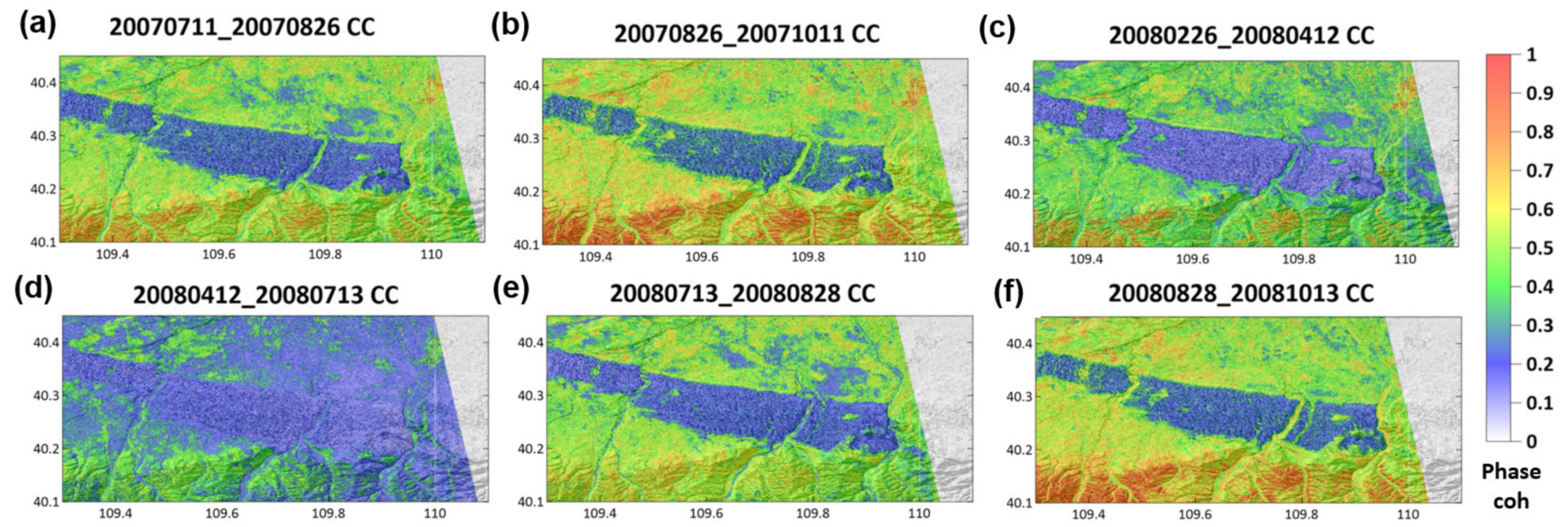
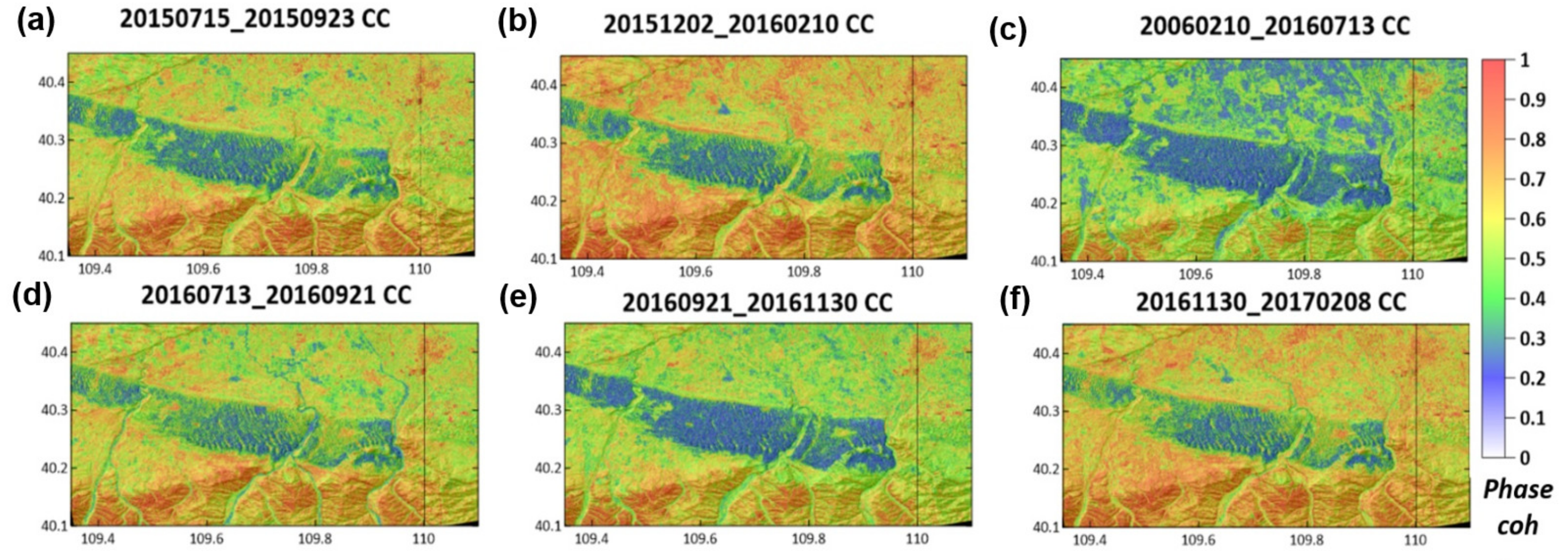
The ALOS PALSAR time series were used for long-term monitoring, while Sentinel-1 imagery tested the availability of short-term AER measurements. Two L-band InSAR image series of PALSAR-1 and -2 were first employed to extract phase coherence maps. A minimum span tree (MST) [65] was formed in which the average of InSAR phase coherence between pairs could be the maximum value, and the InSAR phase coherence between the formed pair was extracted. Phase coherence maps generated by PALSAR-1 InSAR pairs during 2007–2008 represented the decorrelation trend before the activity to combat desertification as shown in Figure 3. On the contrary, Figure 4 generated from the PALSAR-2 InSAR time series in 2016–2017 demonstrated decorrelation status after combating desertification.
Vegetation index EVI derived from the medium resolution (30–50 m/pixel) LANDSAT 5 and 8 data were extracted in the corresponding areas of InSAR observations using Google Earth Engine (GEE), as described later. The scattergrams in Figure 5 demonstrated extremely important results in the correlation between vegetation and phase coherence signals.
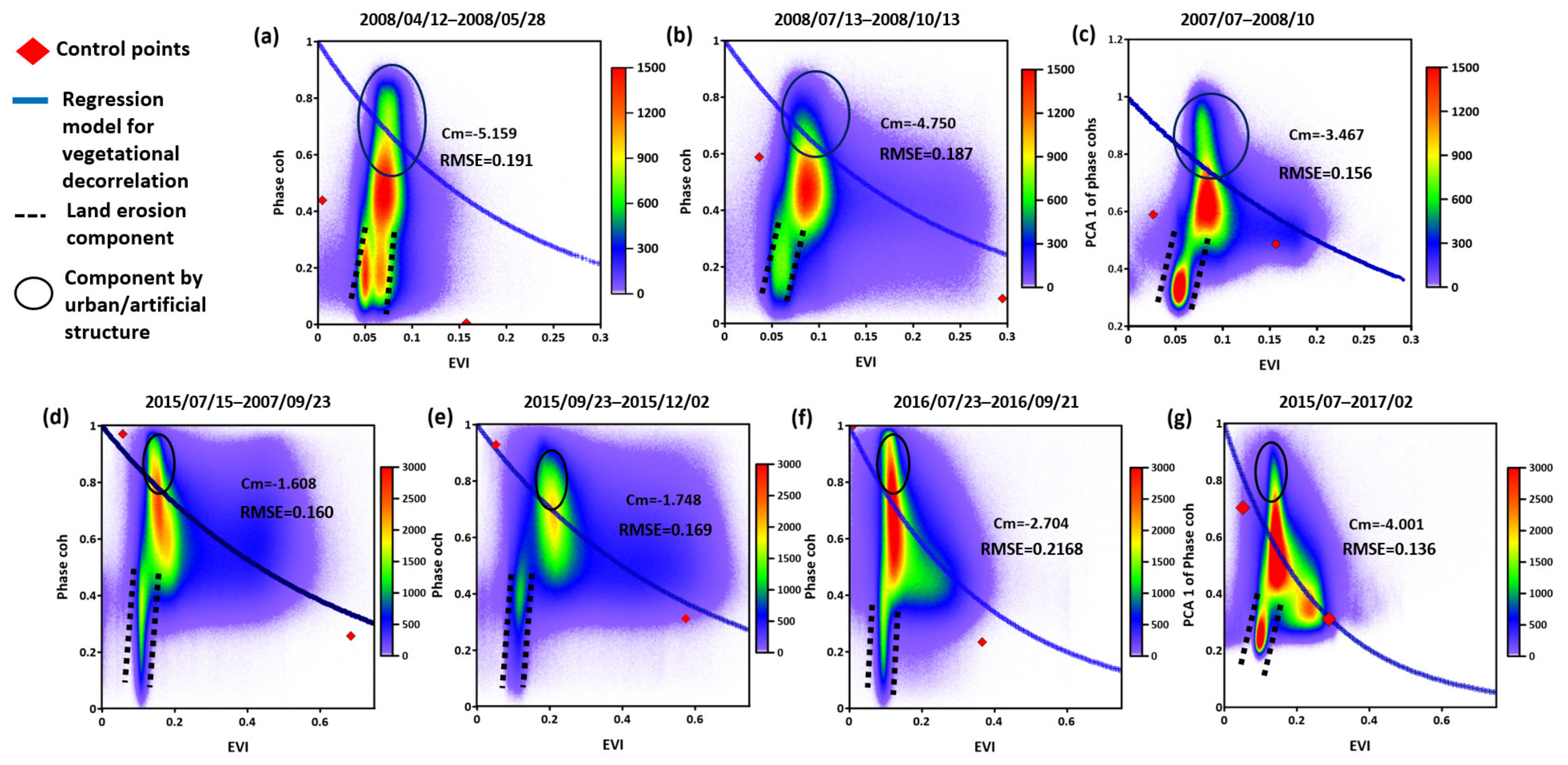
For all the scattergrams illustrated in Figure 5, three components were commonly observed: (1) the component of vegetation which is populated around the decorrelation model (blue lines); (2) elongated part into lower EVI and low phase coherence (black dotted lines); (3) some distribution with low EVI and high phase coherence presented in black ellipses. The components around the modeled decorrelation re clearly vegetated terrains, thus they are decomposed. Elongated components described in (2) with low EVI and low phase coherence assign aeolian erosion, referred to as the erosion component as low vegetation and low phase coherence can only be presented as the erosional surface by the decrease of Zo which induces more aeolian erosion as stated in Section 3.3. Components described in (3) are mainly artificial structures or bare terrain covered by very weak vegetation. The problem we observed here is that the decorrelation model of vegetation was frequently inclined in the component 3 direction when there was no consideration to exclude it from the modeling. Thus, we employed two ways to clarify the findings: (1) processing together with land cover maps, excluding from the modeling some specific land cover types such as water surface, desert, and urban area, which may distort the decorrelation model on vegetation; (2) further introducing two control points in regression modeling, one with low EVI and high phase coherence and the other with high EVI and low phase coherence. Both points were clearly located in natural vegetation, and the value was assigned within a sufficient surrounding buffer zone. These two control points were introduced in the regression with high weighting values. The effects of the control points may not have been significant, but they enabled us to observe the controllability of the regression model. We observed that the regression model of vegetation decorrelation through the posterior process was better established as it was not inclined towards artificial/urban components compared to other cases by a prior processor (refer to Figure 5c,g). Moreover, it is worthwhile highlighting that the erosion components assigned by black dotted lines, which was our main object to measure, were all better distinguished in the results by a posterior process, as shown in Figure 5c,g. The erosion components characterized the inverse relationship between the EVI and phase coherences, which were also observed in precedent studies regarding surface migration on arid sandy desert using phase coherence [28,29,31,32,33]. We measured and presented root mean square errors (RMSEs) between regression models by Equation (5) and observations. Those values demonstrated that the posterior processor was more effective to eradicate uncorrelated components of time-series phase coherence. Which corresponded to the precedent phase coherence analysis by Kim et al. (2021) [50]. The observations summarized above hence formed the basis of using a posterior process to extract AER as the default method.
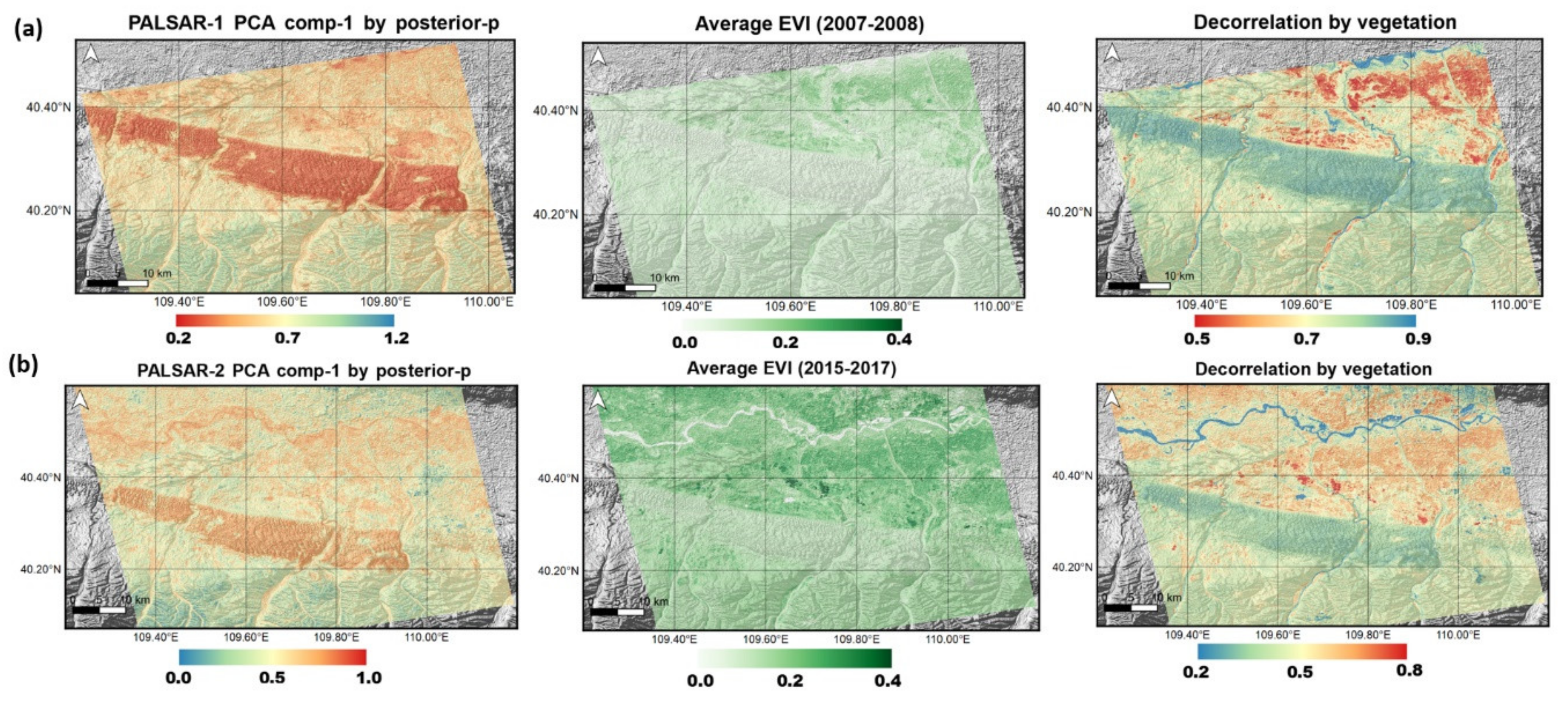
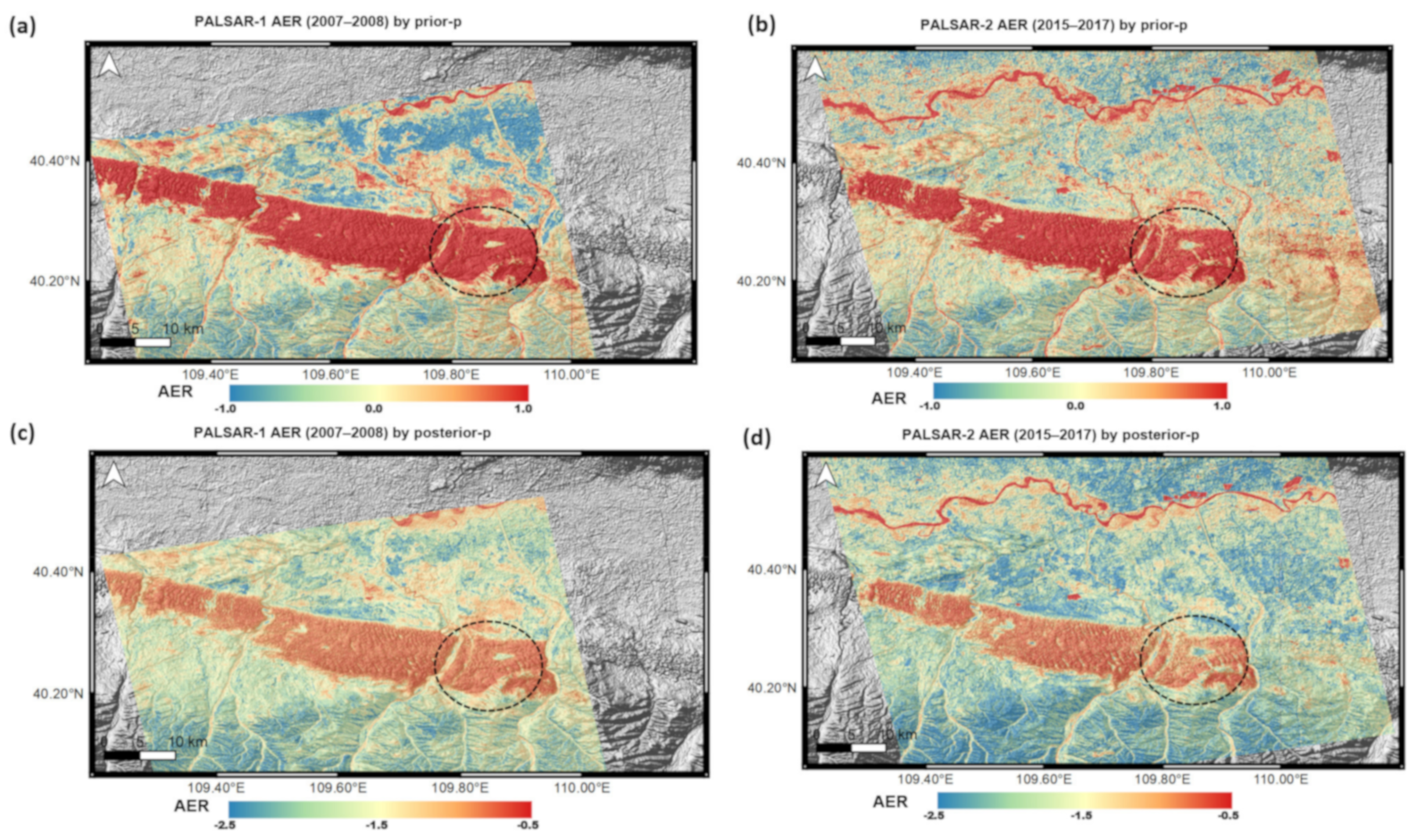
In order to extract the decorrelation component by vegetation, we established a decorrelation map using an established regression model and EVI, as shown in Figure 6. Therefore, we were able to decompose the decorrelation map from phase coherence or the PCA 1st component of the phase coherence time-series, as demonstrated in Figure 7. It should be noted that the AER in Figure 7 is the relative strength of aeolian erosion between the maximum to minimum values after decomposition. Thus, the minimum AER value in an InSAR time-series analysis presents the minimum change of topography while the maximum AER value is the maximum change of topography in each time-series analysis. As we inferred from the Figure 5 cases, the results from a posterior processor showed the outcomes better distinguished the before (see Figure 7c) and after activities to combat desertification (Figure 7d), which were intensively conducted in the mid-2010s.
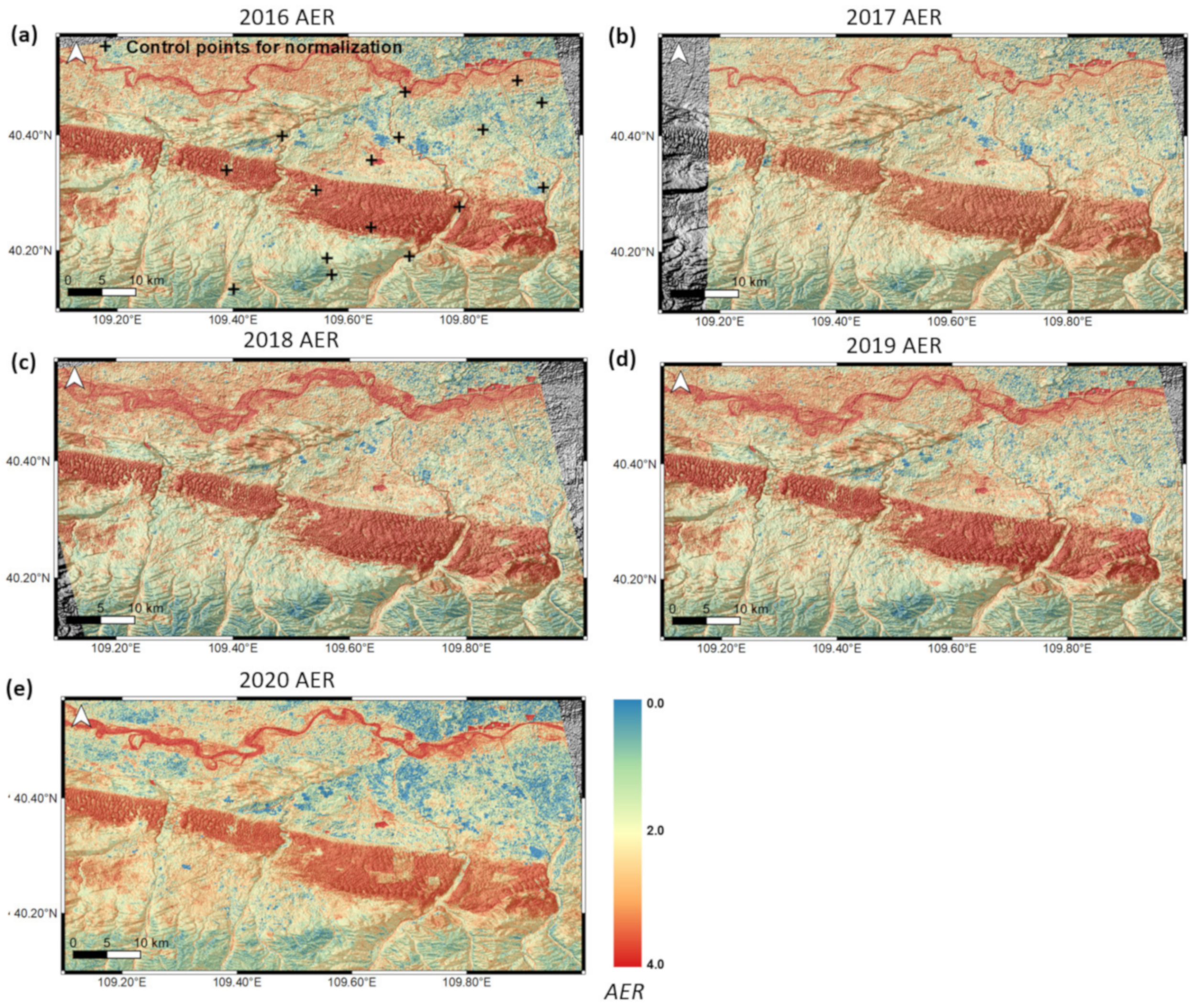
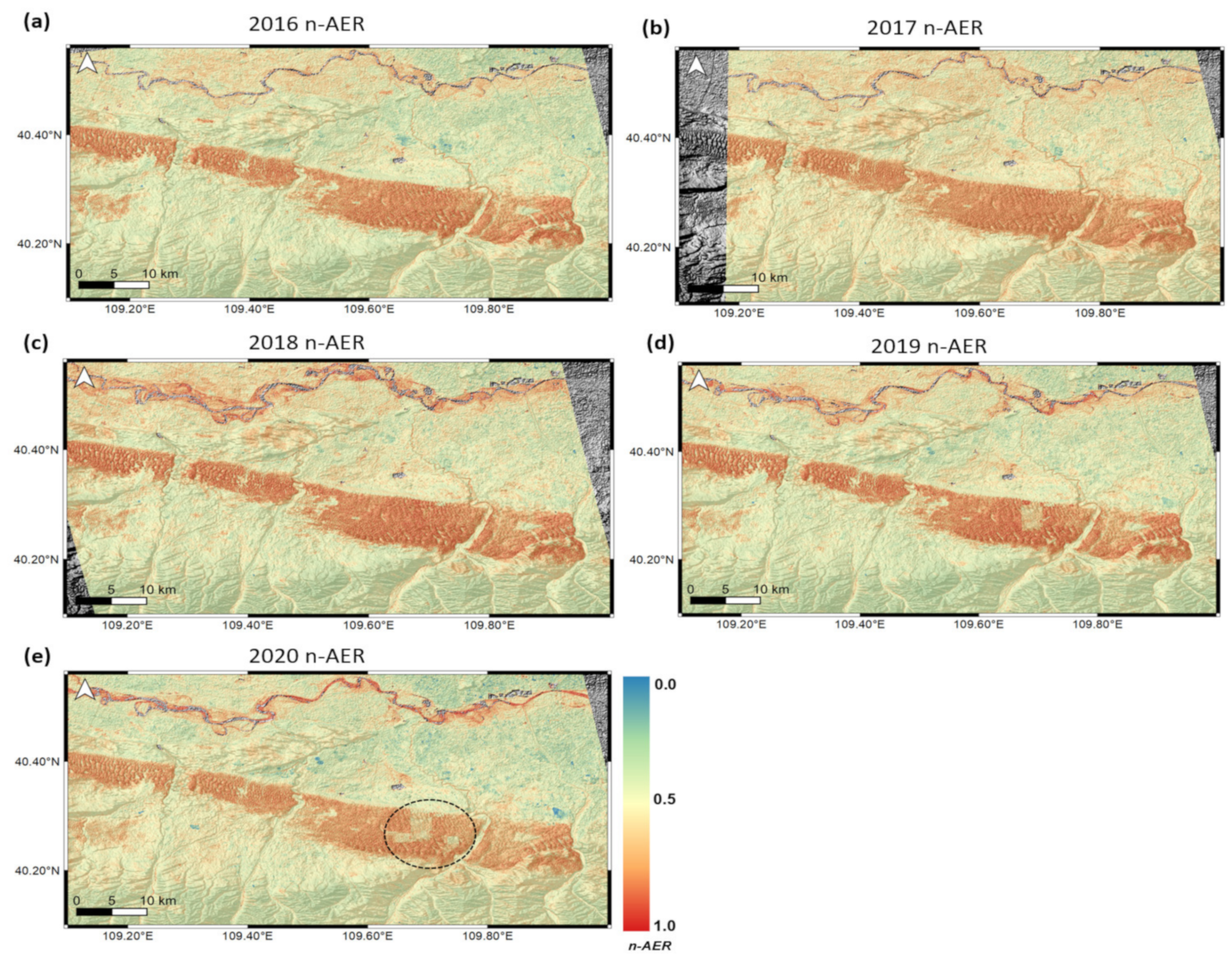
Sentinel-1 InSAR phase coherence time-series covering the 2016–2020 period were constructed in consecutive InSAR pairs. We established short-term time series for each year from 2016 to 2020. After the decomposition of vegetation, surface erosion components in each year were established (Figure 8). Since the erosion map created by a prior processor presented more noise because of temporal variation of the EVI and phase coherence, our default approach followed a posterior decomposition processor in all Sentinel-1 cases. The AER time-series analysis is for the inter-comparison of short-term aeolian erosion using the high temporal density of Sentinel-1 InSAR image acquisitions. Thus, a normalization procedure was necessary to convert all AER metrics in the same data range. The details of validation employing normalized Sentinel-1 AER are described in the next section.
5. Discussion
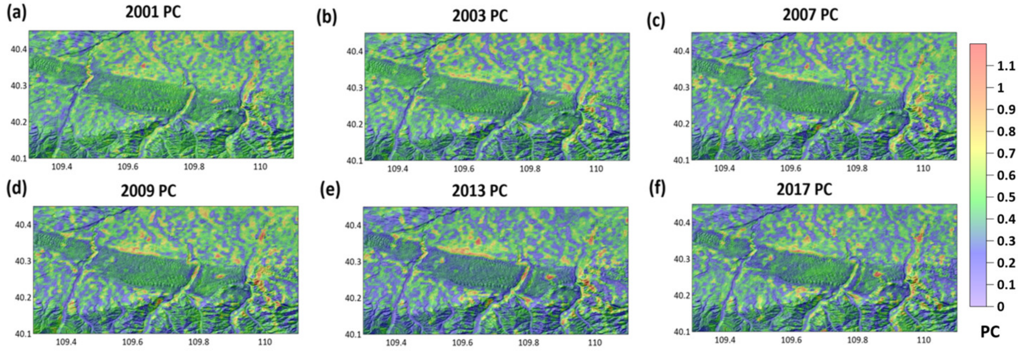
Since the decomposition procedure was conducted based on the vegetation index, it is not ideal to employ other vegetation indicators to assess extracted AER. Thus, we employed the PC for this purpose. The PC time-series representing the surface characteristics in the target area from 2000 to 2017 were reconstructed based on MODIS 43 BRDF products as shown in Figure 9 [66] in which the relatively clear discrimination between sand dune and other land cover types can be clearly observed. Thus, it is worth noting that the PC to InSAR erosion map comparison was effective for validating our approach.
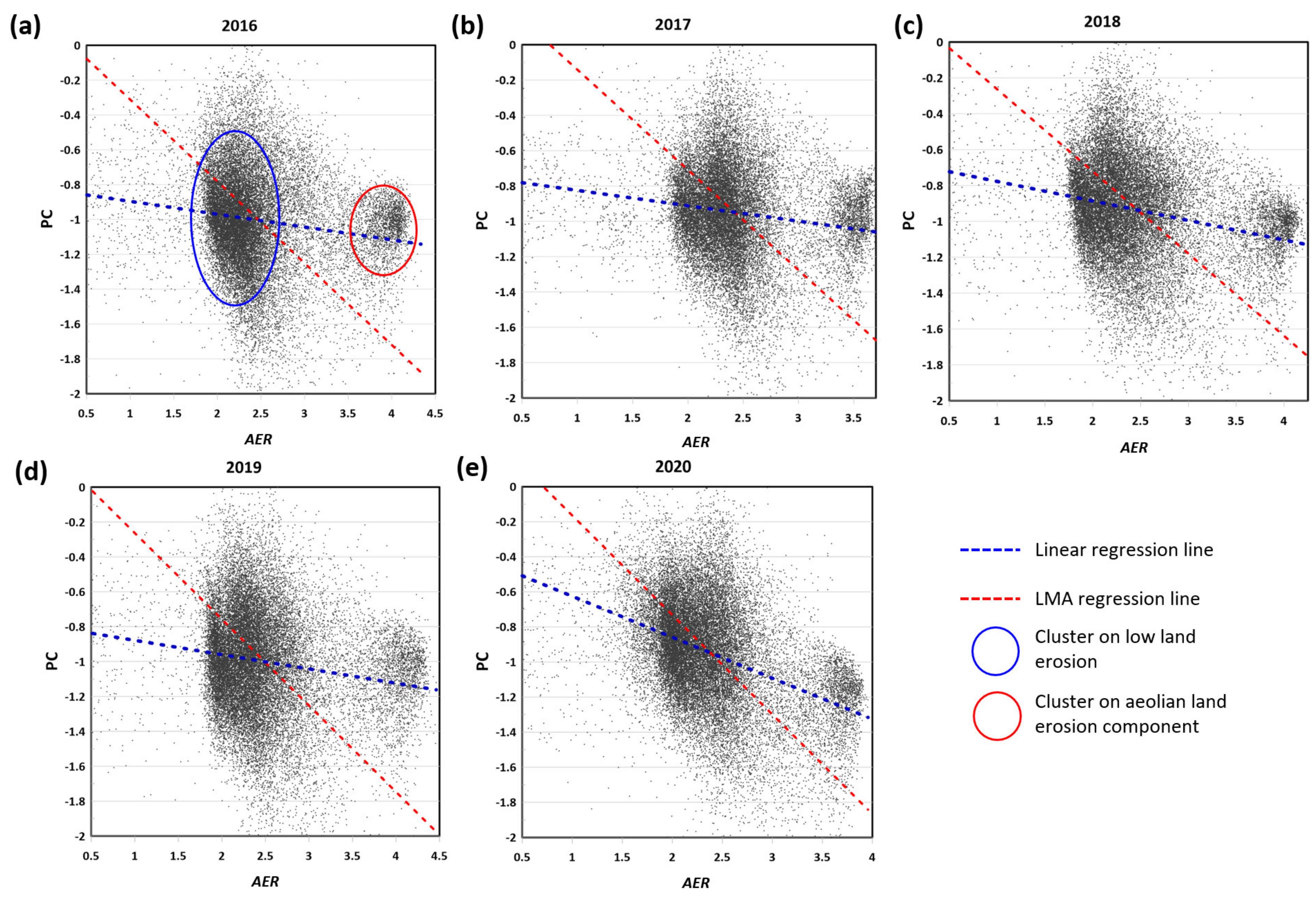
The scattergrams between the PCs and AERs extracted from Sentinel-1 in the 2016–2020 period, together with the established regression models, are shown in Figure 10 and Table 3. It is noted that there are commonly two data clusters (see blue and red ellipses in Figure 10a) together with the inverse proportional relationship in PC-AER distributions. The part encircled by the red ellipse is the aeolian land degradation component, and the part outlined in the blue ellipse represents the weak erosion components with low-to-high rough surfaces, such as vegetation and urban areas. The dispersions in PCs in both distributions mainly originated from resolution differences of the PC (500 m) and the AER (30 m) as aggregated land cover types in one PC pixel which induced a large dispersion. However, parts of the dispersion in the aeolian erosion ellipse can be attributed to the influences of other control factors of aeolian erosion, such as soil moisture, condensation, and clay ratio. The lower half part of the high roughness ellipse, i.e., the lower part in the blue ellipse, is certainly formed by the relatively flat but robust surface to aeolian erosion in rocky areas, concrete pavements, and the roadside; thus they have low PC and low AER values. Other upper parts of the low erosion ellipse can be explained as high roughness in surfaces found in forest and urban structures.
Therefore, the regression models of the AER and PC were not clear in both the least mean squares (LMA) and linear regression approaches as listed in Table 3. Considering the dispersion in low erosion and high erosion ellipses, we estimated that the PC-AER on the natural surface was similar to the linear regression model, which was actually the first-order polynomial presented in Table 3 rather than the high order polynomial cases. High data dispersion in the PC to AER regression showed the extra effects on surface changes such as soil moisture, wind strength, and human activities which induced aeolian erosion. The introduction of advanced biomass metrics that can be extracted from a sequence of new algorithms [67,68] or from new sensing systems [69,70] will be helpful for a precise validation of the AER in future studies. Thus, the developed AER tracing scheme will be useful for the activities to combat desertification as well as the early warning of dust storm generations after applying such precise validation processing.
A further step applied was to normalize all derived AER measurements by different InSAR time-series analyses in the same standardized range. The processed outcomes can be comparable to each so it is referred to as n-AER as stated in Section 1. Regarding normalization, a linear regression model assuming a linear relationship between the values of the reference and subject images for points of the same land cover types as those reported in Sadeghi et al. (2017) [71] was applied in this study. Based on the dark set-bright set (DB) method developed by Hall et al. (1991) [72], a total of 16 erosional ground control points (EGCPs) appearing unchanged as settlement, river, and road were manually selected to derive the normalization coefficients (refer to Figure 8a to see the location of the selected points). Given the pattern of exponential decay in phase coherence presented in Equation (5), a linear relationship can be established:
where G is the gain value, off is offset to deploy logarithmic AER value into a normalized data range, and I is ith target InSAR time series observation. The G and off_set can be extracted from the linear system in Equation (13) and EGCPs were assigned to 0.0 with zero migration over settlement and road and 1.0 with full decorrelation over the water surface. The values of the potential EGCPs in the InSAR AER images over the whole observation period were recorded respectively and chosen carefully only in the case that there were no significant changes. Based on the coefficients, i.e., Gi and off_seti derived through ordinary least squares estimation, the AER images were normalized through a linear transformation. The extracted n-AERs are demonstrated in Figure 11 for ALOS PALSAR 1/2 and in Figure 12 for Sentinel-1.
n-AERi = GiXlog(AERi) + off_seti
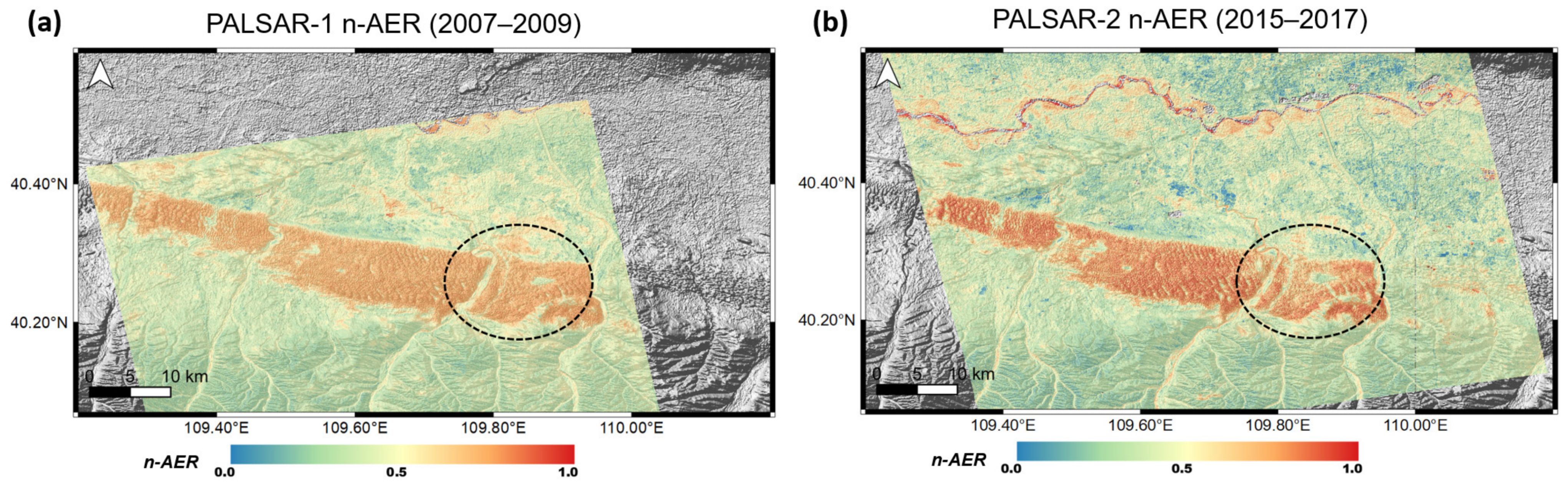
Therefore the n-AER maps produced by independent phase coherence time-series analysis over the Kubuqi Desert demonstrated how the change in surface characteristics caused the mitigation of erosions. A further procedure for assessment of InSAR n-AER products was performed based on the inter-comparison to vegetation information and ground truth regarding activities to combat desertification. The n-AER covering a decadal period in comparison to the EVI of LANDSAT 5/8 and MODIS is presented in Table 4. It was observed that commonly in LANDSAT and MODIS EVIs, the low EVI area (<0.2, 0.15, and 0.1, respectively) was dramatically reduced in the 2016 observations compared to the 2007 observations. For instance, the area with an EVI lower than 0.1 changed from 77% in 2006 to 6.6% in 2016. When the MODIS EVIs were employed to address different sensor issues in the use of LANDSAT 5 and 8, low EVI areas were considerably reduced, especially in areas where the EVI was smaller than 0.1. More importantly, n-AER values in low EVI areas showed no differences, or worse, in the 2007 and 2016 observations. Thus, the values in Table 4 represented that the overall changes in n-AER were due to the increasing vegetation coverages in the entire Kubuqi area. However, natural conditions that induce aeolian land degradation were still severe. Conclusively, it has been proven that the main drivers of mitigating sand dune activities and aeolian land degradation for the last decade have been anthropogenic factors, including activities to combat desertification in this area.
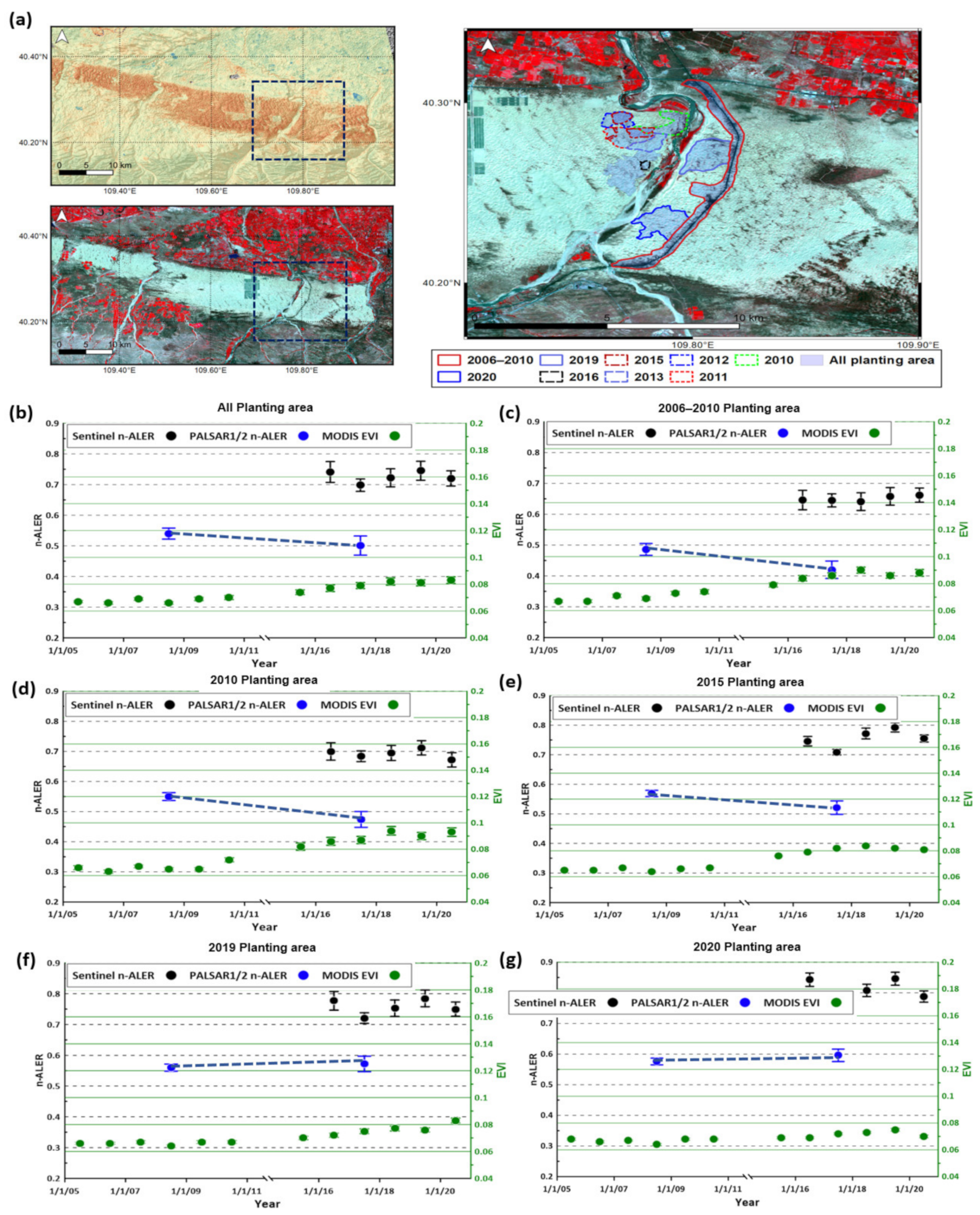
These observations can be proved again by employing ground truth regarding activities to combat desertification. Figure 13a showed the extent of yearly planting areas brought about by efforts to combat desertification conducted by international NGOs and Chinese local government from 2006 to 2020. Figure 13b demonstrated the organized planting efforts that resulted in noticeable changes in both EVI and n-AER values as observed in PALSAR 1/2 time-series analyses covering the 10-year period. On the contrary, the short-term n-AERs by Sentinel-1 from 2016 to 2020 did not make significant changes. Obviously, old planting areas (2006–2010 and 2010) in Figure 13c,d were most successful in reducing aeolian erosion in the decadal period. Compared to the recent planting activities and their relatively weak anti-AER effects presented in Figure 13e–g, it is concluded that the activities to combat desertification during 2006–2010 successfully built a high aerodynamic surface roughness wall crossing Kubuqi Desert, which prevented aeolian saltation.
All these results support that the phase coherence time-series analysis developed in this study is effective in tracing erosion. It has also shown great potential for identifying sources of dust and ongoing erosion by replacing existing approaches such as AOD analysis. Compared to 25 km resolution dust source tracing using AOD analysis, the InSAR phase coherence method provided an improved opportunity to directly observe erosion with a few decameters spatial resolution and better temporal resolution regardless of climate condition. However, it should be noted that the limitations of the phase coherence time-series analysis for dust source mapping are also clear. As mentioned above, the values observed by phase coherence time-series analysis are only relative intensities. Therefore, a calibration process between erosion maps in each epoch using land control points is necessary. Another significant problem of phase coherence analysis is the reliability of the decomposition of the phase coherence contribution by other factors such as vegetation, soil moisture, snow cover, and other land changes. In this respect, we propose a more detailed interpretation of phase coherence time-series that combines high-resolution remote sensing data products such as drone and space-borne ultra-high-resolution products. Cross-comparison studies using climatic factors such as soil moisture, wind speed, and precipitation will provide insight into the improvement of the phase coherence AER.
6. Conclusions and Future Work
This study proved that precise long-term monitoring of aeolian erosion and progress of involved surface condition is feasible using time series InSAR and medium resolution vegetation index products. A scheme employing InSAR phase coherence time-series successfully traced a temporal consequence in which activity to combat desertification caused the increase of aerodynamic roughness length and the decrease of sand dune mobility. In spite of the favorable natural environment for intensive aeolian land degradation in N.W Chinese deserts, the efforts to combat desertification and other anthropogenic factors led to the overall reduction of erosion in Kubuqi during the period 2000–2020. Our scheme successfully reconstructed such a long-term and steady-going combating desertification consequence on the establishment of a blocking wall leading to the effective mitigation of aeolian erosion. Thus, the effectiveness of the phase coherence approach for erosion monitoring was well verified in both aspects of precision and spatio-temporal resolution.
However, it has appeared that a few issues remained to be solved in the proposed scheme before it is to be employed as a standard approach for AER measurement. First, the driven InSAR AER only extracted the relative strength of aeolian erosion; thus, it should be calibrated compared to the metrics of quantitative erosion. On the other hand, the InSAR signal still needs to be further inspected to decompose other governing factors of erosion, such as climatic factors and the footprints of the urban area, rock surface, and concrete resistant land cover that exists against erosion. It means the procedure needs to be more updated considering how surface conditions for erosion are very complicated.
For future work, in order to carry out the quantitative analysis which is more generally applicable for erosion monitoring in major sand dust source areas, it is essential to perform additional measurement over the target area, such as UAV stereo, high-resolution satellite analysis, and close-range photogrammetry. Improved time-series data analysis together with high-resolution products will be of great help for the planning of more effective activity to combat desertification and better prediction and observation of erosion in the arid desert. Future space-borne sensors such as NASA-ISRO Synthetic Aperture Radar (NiSAR) [73], Geostationary Ocean Color Imager-2 (GOCI-2) [74], and Panchromatic Remote-sensing Instrument for Stereo Mapping-2 (PRISM-2) will provide highly valuable data sets to update or precisely validate proposed algorithms.
Author Contributions
J.-R.K. developed algorithms and wrote major part of draft. C.-W.L. conducted InSAR processing and time series analysis of other data sets. S.-Y.L. was charge of normalization and corresponding writing together with summarizing of draft. All authors have read and agreed to the published version of the manuscript.
Funding
The authors acknowledge support by the Ministry of Science and Technology (MOST) in Taiwan. This research received partial funding for S.-Y.L. under grant number MOST 110-2119-M-004-001 to support APC.
Data Availability Statement
The data in this study are available on request from the corresponding author.
Acknowledgments
This study was conducted by the support of Korean Forest service. The research activities in the target area were kindly supported by Future Forest (http://www.futureforest.org/ (accessed on 1 June 2021)), United Nations Convention to Combat Desertification (UNCCD) and China Youth League. ALOS PALSAR data is kindly provided by 6th Research Announcement of Japan Aerospace Exploration Agency (JAXA).
Conflicts of Interest
The authors declare no conflict of interest. The funders had no role in the design of the study; in the collection, analyses, or interpretation of data; in the writing of the manuscript, or in the decision to publish the results.
References
- Tegen, I.; Fung, I. Contribution to the atmospheric mineral aerosol load from land surface modification. J. Geophys. Res. Atmos. 1995, 100, 18707–18726. [Google Scholar] [CrossRef]
- Xuan, J.; Sokolik, I.N.; Hao, J.; Guo, F.; Mao, H.; Yang, G. Identification and characterization of sources of atmospheric mineral dust in East Asia. Atmos. Environ. 2004, 38, 6239–6252. [Google Scholar] [CrossRef]
- Wang, X.; Huang, J.; Ji, M.; Higuchi, K. Variability of East Asia dust events and their long-term trend. Atmos. Environ. 2008, 42, 3156–3165. [Google Scholar] [CrossRef]
- Kurosaki, Y.; Mikami, M. Regional difference in the characteristic of dust event in East Asia: Relationship among dust outbreak, surface wind, and land surface condition. J. Meteorol. Soc. Japan. Ser. II 2005, 83, 1–18. [Google Scholar] [CrossRef] [Green Version]
- Zhang, B.; Tsunekawa, A.; Tsubo, M. Contributions of sandy lands and stony deserts to long-distance dust emission in China and Mongolia during 2000–2006. Glob. Planet. Chang. 2008, 60, 487–504. [Google Scholar] [CrossRef]
- Kim, J. Transport routes and source regions of Asian dust observed in Korea during the past 40 years (1965–2004). Atmos. Environ. 2008, 42, 4778–4789. [Google Scholar] [CrossRef]
- Bryant, R.G.; Bigg, G.R.; Mahowald, N.M.; Eckardt, F.D.; Ross, S.G. Dust emission response to climate in southern Africa. J. Geophys. Res. Atmos. 2007, 112. [Google Scholar] [CrossRef] [Green Version]
- Kaskaoutis, D.; Kosmopoulos, P.; Nastos, P.; Kambezidis, H.; Sharma, M.; Mehdi, W. Transport pathways of Sahara dust over Athens, Greece as detected by MODIS and TOMS. Geomat. Nat. Hazards Risk 2012, 3, 35–54. [Google Scholar] [CrossRef]
- Prasad, A.K.; Singh, R.P. Changes in aerosol parameters during major dust storm events (2001–2005) over the Indo-Gangetic Plains using AERONET and MODIS data. J. Geophys. Res. Atmos. 2007, 112. [Google Scholar] [CrossRef] [Green Version]
- Ginoux, P.; Prospero, J.M.; Gill, T.E.; Hsu, N.C.; Zhao, M. Global-scale attribution of anthropogenic and natural dust sources and their emission rates based on MODIS Deep Blue aerosol products. Rev. Geophys. 2012, 50. [Google Scholar] [CrossRef]
- United Nations Convention to Combart Desertification Addressing Sand and Dust Strom in SDG Implementation. Available online: https://knowledge.unccd.int/publications/addressing-sand-and-dust-storms-sdg-implementation (accessed on 1 June 2021).
- Du, H.; Wang, T.; Xue, X.; Li, S. Modelling of sand/dust emission in Northern China from 2001 to 2014. Geoderma 2012, 330, 162–176. [Google Scholar] [CrossRef]
- Du, H.; Xue, X.; Wang, T. Estimation of saltation emission in the Kubuqi Desert, North China. Sci. Total Environ. 2014, 479, 77–92. [Google Scholar] [CrossRef]
- Sun, J.; Zhang, M.; Liu, T. Spatial and temporal characteristics of dust storms in China and its surrounding regions, 1960–1999: Relations to source area and climate. J. Geophys. Res. Atmos. 2001, 106, 10325–10333. [Google Scholar] [CrossRef]
- Zhang, B.; Tsunekawa, A.; Tsubo, M. Identification of dust hot spots from multi-resolution remotely sensed data in eastern China and Mongolia. Water Air Soil Pollut. 2015, 226, 117. [Google Scholar] [CrossRef]
- Wang, X.; Eerdun, H.; Zhou, Z.; Liu, X. Significance of variations in the wind energy environment over the past 50 years with respect to dune activity and desertification in arid and semiarid northern China. Geomorphology 2007, 86, 252–266. [Google Scholar] [CrossRef]
- Wang, X.; Yang, Y.; Dong, Z.; Zhang, C. Responses of dune activity and desertification in China to global warming in the twenty-first century. Glob. Planet. Chang. 2009, 67, 167–185. [Google Scholar] [CrossRef]
- Yu, X.; Zhuo, Y.; Liu, H.; Wang, Q.; Wen, L.; Li, Z.; Liang, C.; Wang, L. Degree of desertification based on normalized landscape index of sandy lands in inner Mongolia, China. Glob. Ecol. Conserv. 2020, 23, e01132. [Google Scholar] [CrossRef]
- Liu, L.; Skidmore, E.; Hasi, E.; Wagner, L.; Tatarko, J. Dune sand transport as influenced by wind directions, speed and frequencies in the Ordos Plateau, China. Geomorphology 2005, 67, 283–297. [Google Scholar] [CrossRef]
- Yun, J.; Kim, J.; Choi, Y.; Yun, H. Monitoring of desert dune topography by multi angle sensors. AGUFM 2011, 2011, EP31A-0794. [Google Scholar]
- Yang, X.; Forman, S.; Hu, F.; Zhang, D.; Liu, Z.; Li, H. Initial insights into the age and origin of the Kubuqi sand sea of northern China. Geomorphology 2016, 259, 30–39. [Google Scholar] [CrossRef]
- Hermas, E.; Leprince, S.; Abou El-Magd, I. Retrieving sand dune movements using sub-pixel correlation of multi-temporal optical remote sensing imagery, northwest Sinai Peninsula, Egypt. Remote Sens. Environ. 2012, 121, 51–60. [Google Scholar] [CrossRef]
- Yao, Z.; Wang, T.; Han, Z.; Zhang, W.; Zhao, A. Migration of sand dunes on the northern Alxa Plateau, Inner Mongolia, China. J. Arid Environ. 2007, 70, 80–93. [Google Scholar] [CrossRef]
- Mahmoud, A.M.A.; Novellino, A.; Hussain, E.; Marsh, S.; Psimoulis, P.; Smith, M. The use of SAR offset tracking for detecting sand dune movement in Sudan. Remote Sens. 2020, 12, 3410. [Google Scholar] [CrossRef]
- Solazzo, D.; Sankey, J.B.; Sankey, T.T.; Munson, S.M. Mapping and measuring aeolian sand dunes with photogrammetry and LiDAR from unmanned aerial vehicles (UAV) and multispectral satellite imagery on the Paria Plateau, AZ, USA. Geomorphology 2018, 319, 174–185. [Google Scholar] [CrossRef]
- Laporte-Fauret, Q.; Marieu, V.; Castelle, B.; Michalet, R.; Bujan, S.; Rosebery, D. Low-Cost UAV for high-resolution and large-scale coastal dune change monitoring using photogrammetry. J. Mar. Sci. Eng. 2019, 7, 63. [Google Scholar] [CrossRef] [Green Version]
- Grohmann, C.H.; Garcia, G.P.; Affonso, A.A.; Albuquerque, R.W. Dune migration and volume change from airborne LiDAR, terrestrial LiDAR and Structure from Motion-Multi View Stereo. Comput. Geosci. 2020, 143, 104569. [Google Scholar] [CrossRef]
- Liu, J.G.; Black, A.; Lee, H.; Hanaizumi, H.; Moore, J.M. Land surface change detection in a desert area in Algeria using multi-temporal ERS SAR coherence images. Int. J. Remote Sens. 2001, 22, 2463–2477. [Google Scholar] [CrossRef]
- Wegmuller, U.; Strozzi, T.; Farr, T.; Werner, C.L. Arid land surface characterization with repeat-pass SAR interferometry. IEEE Trans. Geosci. Remote Sens. 2000, 38, 776–781. [Google Scholar] [CrossRef]
- Gómez, D.; Salvador, P.; Sanz, J.; Casanova, C.; Casanova, J.L. Detecting Areas Vulnerable to Sand Encroachment Using Remote Sensing and GIS Techniques in Nouakchott, Mauritania. Remote Sens. 2018, 10, 1541. [Google Scholar] [CrossRef] [Green Version]
- Havivi, S.; Amir, D.; Schvartzman, I.; August, Y.; Maman, S.; Rotman, S.R.; Blumberg, D.G. Mapping dune dynamics by InSAR coherence. Earth Surf. Process. Landf. 2018, 43, 1229–1240. [Google Scholar] [CrossRef]
- Ullmann, T.; Sauerbrey, J.; Hoffmeister, D.; May, S.M.; Baumhauer, R.; Bubenzer, O. Assessing Spatiotemporal Variations of Sentinel-1 InSAR Coherence at Different Time Scales over the Atacama Desert (Chile) between 2015 and 2018. Remote Sens. 2019, 11, 2960. [Google Scholar] [CrossRef] [Green Version]
- Santoro, M.; Askne, J.I.; Wegmuller, U.; Werner, C.L. Observations, modeling, and applications of ERS-ENVISAT coherence over land surfaces. IEEE Trans. Geosci. Remote Sens. 2007, 45, 2600–2611. [Google Scholar] [CrossRef]
- Askne, J.I.; Dammert, P.B.; Ulander, L.M.; Smith, G. C-band repeat-pass interferometric SAR observations of the forest. IEEE Trans. Geosci. Remote Sens. 1997, 35, 25–35. [Google Scholar] [CrossRef]
- Askne, J.; Santoro, M. Multitemporal repeat pass SAR interferometry of boreal forests. IEEE Trans. Geosci. Remote Sens. 2005, 43, 1219–1228. [Google Scholar] [CrossRef]
- Wang, T.; Liao, M.; Perissin, D. InSAR coherence-decomposition analysis. IEEE Geosci. Remote Sens. Lett. 2009, 7, 156–160. [Google Scholar] [CrossRef]
- Zalite, K.; Antropov, O.; Praks, J.; Voormansik, K.; Noorma, M. Monitoring of agricultural grasslands with time series of X-band repeat-pass interferometric SAR. IEEE J. Sel. Top. Appl. Earth Obs. Remote Sens. 2015, 9, 3687–3697. [Google Scholar] [CrossRef]
- Ahmed, R.; Siqueira, P.; Hensley, S.; Chapman, B.; Bergen, K. A survey of temporal decorrelation from spaceborne L-Band repeat-pass InSAR. Remote Sens. Environ. 2011, 115, 2887–2896. [Google Scholar] [CrossRef]
- Zebker, H.A.; Villasenor, J. Decorrelation in interferometric radar echoes. IEEE Trans. Geosci. Remote Sens. 1992, 30, 950–959. [Google Scholar] [CrossRef] [Green Version]
- Just, D.; Bamler, R. Phase statistics of interferograms with applications to synthetic aperture radar. Appl. Opt. 1994, 33, 4361–4368. [Google Scholar] [CrossRef]
- Tamm, T.; Zalite, K.; Voormansik, K.; Talgre, L. Relating Sentinel-1 interferometric coherence to mowing events on grasslands. Remote Sens. 2016, 8, 802. [Google Scholar] [CrossRef] [Green Version]
- Wei, M.; Sandwell, D.T. Decorrelation of L-band and C-band interferometry over vegetated areas in California. IEEE Trans. Geosci. Remote Sens. 2010, 48, 2942–2952. [Google Scholar]
- Rosenqvist, A.; Shimada, M.; Ito, N.; Watanabe, M. ALOS PALSAR: A pathfinder mission for global-scale monitoring of the environment. IEEE Trans. Geosci. Remote Sens. 2007, 45, 3307–3316. [Google Scholar] [CrossRef]
- Rosenqvist, A.; Shimada, M.; Suzuki, S.; Ohgushi, F.; Tadono, T.; Watanabe, M.; Tsuzuku, K.; Watanabe, T.; Kamijo, S.; Aoki, E. Operational performance of the ALOS global systematic acquisition strategy and observation plans for ALOS-2 PALSAR-2. Remote Sens. Environ. 2014, 155, 3–12. [Google Scholar] [CrossRef]
- Geudtner, D.; Torres, R.; Snoeij, P.; Davidson, M.; Rommen, B. Sentinel-1 system capabilities and applications. In Proceedings of the 2014 IEEE Geoscience and Remote Sensing Symposium, Quebec City, QC, Canada, 13–18 July 2014; pp. 1457–1460. [Google Scholar]
- Torres, R.; Snoeij, P.; Geudtner, D.; Bibby, D.; Davidson, M.; Attema, E.; Potin, P.; Rommen, B.; Floury, N.; Brown, M. GMES Sentinel-1 mission. Remote Sens. Environ. 2012, 120, 9–24. [Google Scholar] [CrossRef]
- Lee, C.-W.; Lu, Z.; Jung, H.-S. Simulation of time-series surface deformation to validate a multi-interferogram InSAR processing technique. Int. J. Remote Sens. 2012, 33, 7075–7087. [Google Scholar] [CrossRef]
- Yun, H.-W.; Kim, J.-R.; Choi, Y.-S.; Lin, S.-Y. Analyses of Time Series InSAR Signatures for Land Cover Classification: Case Studies over Dense Forestry Areas with L-Band SAR Images. Sensors 2019, 19, 2830. [Google Scholar] [CrossRef] [Green Version]
- Gallagher, N.B.; O’Sullivan, D.; Palacios, M. The Effect of Data Centering on PCA Models. 2020. Available online: https://eigenvector.com/ (accessed on 1 June 2021).
- Kim, J.; Dorjsuren, M.; Choi, Y.; Purevjav, G. Reconstructed Aeolian Surface Erosion in Southern Mongolia by Multi-Temporal InSAR Phase Coherence Analyses. Front. Earth Sci 2020, 8, 531104. [Google Scholar] [CrossRef]
- Santoro, M.; Wegmuller, U.; Askne, J.I. Signatures of ERS–Envisat interferometric SAR coherence and phase of short vegetation: An analysis in the case of maize fields. IEEE Trans. Geosci. Remote Sens. 2009, 48, 1702–1713. [Google Scholar] [CrossRef]
- Zhengxing, W.; Chuang, L.; Alfredo, H. From AVHRR-NDVI to MODIS-EVI: Advances in vegetation index research. Acta Ecol. Sin. 2003, 23, 979–987. [Google Scholar]
- Huete, A.R.; Liu, H.; van Leeuwen, W.J. The use of vegetation indices in forested regions: Issues of linearity and saturation. In Proceedings of the IGARSS’97, 1997 IEEE International Geoscience and Remote Sensing Symposium Proceedings. Remote Sensing-A Scientific Vision for Sustainable Development, Singapore, 3–8 August 1997; pp. 1966–1968. [Google Scholar]
- Tian, X.; Li, Z.; Van der Tol, C.; Su, Z.; Li, X.; He, Q.; Bao, Y.; Chen, E.; Li, L. Estimating zero-plane displacement height and aerodynamic roughness length using synthesis of LiDAR and SPOT-5 data. Remote Sens. Environ. 2011, 115, 2330–2341. [Google Scholar] [CrossRef]
- Faivre, R.; Colin, J.; Menenti, M. Evaluation of methods for aerodynamic roughness length retrieval from very high-resolution imaging lidar observations over the Heihe Basin in China. Remote Sens. 2017, 9, 63. [Google Scholar] [CrossRef] [Green Version]
- Colin, J.; Faivre, R. Aerodynamic roughness length estimation from very high-resolution imaging LIDAR observations over the Heihe basin in China. Hydrol. Earth Syst. Sci. Discuss. 2010, 7, 2661–2669. [Google Scholar] [CrossRef] [Green Version]
- Bastiaanssen, W.G.; Menenti, M.; Feddes, R.; Holtslag, A. A remote sensing surface energy balance algorithm for land (SEBAL). 1. Formulation. J. Hydrol. 1998, 212, 198–212. [Google Scholar] [CrossRef]
- Choudhury, B.J.; Monteith, J. A four-layer model for the heat budget of homogeneous land surfaces. Q. J. R. Meteorol. Soc. 1988, 114, 373–398. [Google Scholar] [CrossRef]
- Hautecœur, O.; Leroy, M.M. Surface bidirectional reflectance distribution function observed at global scale by POLDER/ADEOS. Geophys. Res. Lett. 1998, 25, 4197–4200. [Google Scholar] [CrossRef] [Green Version]
- Wanner, W.; Li, X.; Strahler, A. On the derivation of kernels for kernel-driven models of bidirectional reflectance. J. Geophys. Res. Atmos. 1995, 100, 21077–21089. [Google Scholar] [CrossRef]
- Lucht, W.; Roujean, J.L. Considerations in the parametric modeling of BRDF and albedo from multiangular satellite sensor observations. Remote Sens. Rev. 2000, 18, 343–379. [Google Scholar] [CrossRef]
- Marticorena, B.; Chazette, P.; Bergametti, G.; Dulac, F.; Legrand, M. Mapping the aerodynamic roughness length of desert surfaces from the POLDER/ADEOS bi-directional reflectance product. Int. J. Remote Sens. 2004, 25, 603–626. [Google Scholar] [CrossRef]
- Chappell, A.; Webb, N.P.; Guerschman, J.P.; Thomas, D.T.; Mata, G.; Handcock, R.N.; Leys, J.F.; Butler, H.J. Improving ground cover monitoring for wind erosion assessment using MODIS BRDF parameters. Remote Sens. Environ. 2018, 204, 756–768. [Google Scholar] [CrossRef]
- Waggoner, D.G.; Sokolik, I.N. Seasonal dynamics and regional features of MODIS-derived land surface characteristics in dust source regions of East Asia. Remote Sens. Environ. 2010, 114, 2126–2136. [Google Scholar] [CrossRef]
- Refice, A.; Bovenga, F.; Nutricato, R. MST-based stepwise connection strategies for multipass radar data, with application to coregistration and equalization. IEEE Trans. Geosci. Remote Sens. 2006, 44, 2029–2040. [Google Scholar] [CrossRef]
- Strahler, A.H.; Muller, J.; Lucht, W.; Schaaf, C.; Tsang, T.; Gao, F.; Li, X.; Lewis, P.; Barnsley, M.J. MODIS BRDF/albedo product: Algorithm theoretical basis document version 5.0. MODIS Doc. 1999, 23, 42–47. [Google Scholar]
- Lee, S.J.; Kim, J.R.; Choi, Y.S. The extraction of forest CO2 storage capacity using high-resolution airborne LiDAR data. GIScience Remote Sens. 2013, 50, 154–171. [Google Scholar] [CrossRef]
- Li, M.; Im, J.; Quackenbush, L.J.; Liu, T. Forest biomass and carbon stock quantification using airborne LiDAR data: A case study over Huntington Wildlife Forest in the Adirondack Park. IEEE J. Sel. Top. Appl. Earth Obs. Remote Sens. 2014, 7, 3143–3156. [Google Scholar] [CrossRef]
- Narine, L.L.; Popescu, S.; Neuenschwander, A.; Zhou, T.; Srinivasan, S.; Harbeck, K. Estimating aboveground biomass and forest canopy cover with simulated ICESat-2 data. Remote Sens. Environ. 2019, 224, 1–11. [Google Scholar] [CrossRef]
- Duncanson, L.; Neuenschwander, A.; Hancock, S.; Thomas, N.; Fatoyinbo, T.; Simard, M.; Silva, C.A.; Armston, J.; Luthcke, S.B.; Hofton, M. Biomass estimation from simulated GEDI, ICESat-2 and NISAR across environmental gradients in Sonoma County, California. Remote Sens. Environ. 2020, 242, 111779. [Google Scholar] [CrossRef]
- Sadeghi, V.; Ahmadi, F.F.; Ebadi, H. A new automatic regression-based approach for relative radiometric normalization of multitemporal satellite imagery. Comput. Appl. Math. 2017, 36, 825–842. [Google Scholar] [CrossRef]
- Hall, F.G.; Strebel, D.E.; Nickeson, J.E.; Goetz, S.J. Radiometric rectification: Toward a common radiometric response among multidate, multisensor images. Remote Sens. Environ. 1991, 35, 11–27. [Google Scholar] [CrossRef]
- Rosen, P.; Hensley, S.; Shaffer, S.; Edelstein, W.; Kim, Y.; Kumar, R.; Misra, T.; Bhan, R.; Sagi, R. The NASA-ISRO SAR (NISAR) mission dual-band radar instrument preliminary design. In Proceedings of the 2017 IEEE international geoscience and remote sensing symposium (IGARSS), Fort Worth, TX, USA, 23–28 July 2017; pp. 3832–3835. [Google Scholar]
- Kim, J.; Jeong, U.; Ahn, M.-H.; Kim, J.H.; Park, R.J.; Lee, H.; Song, C.H.; Choi, Y.-S.; Lee, K.-H.; Yoo, J.-M. New era of air quality monitoring from space: Geostationary Environment Monitoring Spectrometer (GEMS). Bull. Am. Meteorol. Soc. 2020, 101, E1–E22. [Google Scholar] [CrossRef] [Green Version]
Figure 1.
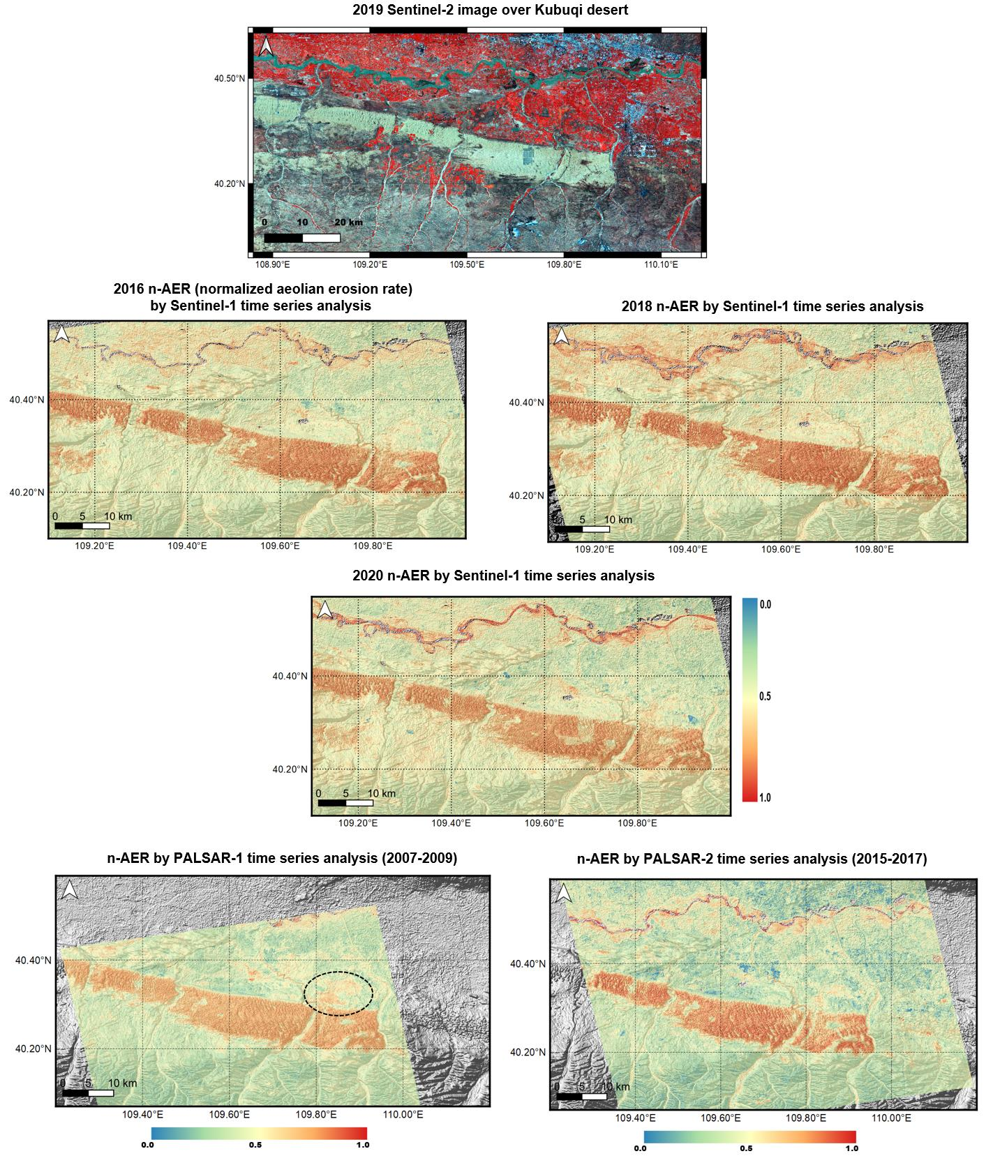
(a) North-Eastern deserts in China. Kubuqi is located on the eastern side. (b) Location and geological context of the target area over Kubuqi. (c) 17 July 2007 (Near-IR-G-B) LANDSAT-5 image and land cover classification. (d) 12 September 2019 (Near-IR-G-B) Sentinel-2 multispectral image and the associated land cover classification. Land cover classification was performed by a maximum likelihood algorithm. The changes in land cover around desert areas were noticed. The land cover classification results were employed in the aeolian erosion rate (AER) extraction process (see Section 3).
Figure 1.
(a) North-Eastern deserts in China. Kubuqi is located on the eastern side. (b) Location and geological context of the target area over Kubuqi. (c) 17 July 2007 (Near-IR-G-B) LANDSAT-5 image and land cover classification. (d) 12 September 2019 (Near-IR-G-B) Sentinel-2 multispectral image and the associated land cover classification. Land cover classification was performed by a maximum likelihood algorithm. The changes in land cover around desert areas were noticed. The land cover classification results were employed in the aeolian erosion rate (AER) extraction process (see Section 3).

Figure 2.
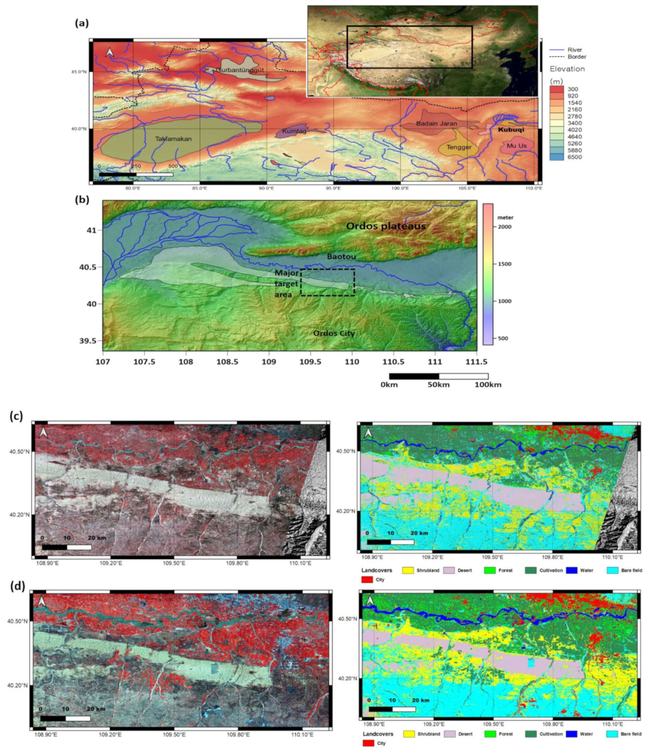
(a) Processing flow of phase coherence analyses for the establishment of the AER map using decomposed phase coherence, which is called a prior processor, (b) Processing flow of phase coherence analyses for the establishment of the AER map using the 1st principal component analysis (PCA) component and its decomposition, which is hereafter referred to as the posterior processor.
Figure 2.
(a) Processing flow of phase coherence analyses for the establishment of the AER map using decomposed phase coherence, which is called a prior processor, (b) Processing flow of phase coherence analyses for the establishment of the AER map using the 1st principal component analysis (PCA) component and its decomposition, which is hereafter referred to as the posterior processor.

Figure 3.
Interferometric Synthetic Aperture Radar (InSAR) phase coherence using PALSAR-1 during the 2007–2008 period, including (a) 11 July 2007–26 August 2007, (b) 26 August 2007–11 October 2007, (c) 26 February 2008–12 April 2008, (d) 12 April 2008–13 July 2008, (e) 13 July 2008–28 August 2008, and (f) 28 August 2008–13 October 2008. Note the dust storm season is usually from February to May, but mainly in March and April.

Figure 4.
InSAR phase coherence using PALSAR-2, including pairs of (a) 15 July 2015–23 September 2015, (b) 2 December 2015–10 February 2016, (c) 10 February 2016–13 July 2016, (d) 13 July 2016–21 September 2016, (e) 21 September 2016–30 November 2016, and (f) 30 November 2016–8 February 2017.
Figure 4.
InSAR phase coherence using PALSAR-2, including pairs of (a) 15 July 2015–23 September 2015, (b) 2 December 2015–10 February 2016, (c) 10 February 2016–13 July 2016, (d) 13 July 2016–21 September 2016, (e) 21 September 2016–30 November 2016, and (f) 30 November 2016–8 February 2017.

Figure 5.
(a,b) The scattergram between the Enhanced Vegetation Index (EVI) and its corresponding single-phase coherence from the PALSAR-1 InSAR pair by a prior processor, (c) The scattergram between the EVI and PCA 1st component from the PALSAR-1 phase coherence time-series by a posterior processor, (d–f) The scattergram between the EVI and its corresponding single-phase coherence from the PALSAR-2 InSAR pair by a prior processor, (g) The scattergram between the EVI and PCA 1st component from the PALSAR-2 phase coherence time-series by a posterior processor. The corresponding regression models were presented as blues lines. Control points indicating high EVI, low phase coherence, and low EVI and high phase coherence were indicated by red points. The color represents the cumulative pixel number of the corresponding EVI-PCA bin. RMSEs were measured over the upper area of the land erosion component and demonstrated with the regression model constant Cm of Equation (1).

Figure 6.
(a) Pre-decomposition stage in PALSAR-1 (2007–2008 period) by a posterior processor. (b) Pre-decomposition stage in PALSAR-2 (2015–2017 period) by a posterior processor with LANDSAT-8 EVI average. The left is the PCA component 1 of PALSAR-1/2 phase coherence, the middle corresponds to the LANDSAT-5/8 EVI average over the InSAR observation time period, and the right is the simulated decorrelation map by vegetation decorrelation model and the EVI map.

Figure 7.
AER maps using ALOS PALSAR-1/2 during 2007–2008 and 2015–2017 periods using a prior processor in (a,b) and a posterior processor in (c,d). Noted that the effects of combating desertification activities are obvious in the posterior processor cases.
Figure 7.
AER maps using ALOS PALSAR-1/2 during 2007–2008 and 2015–2017 periods using a prior processor in (a,b) and a posterior processor in (c,d). Noted that the effects of combating desertification activities are obvious in the posterior processor cases.

Figure 8.
(a–e) Surface erosion map using Sentinel-1 during the 2016–2020 period. Noted that all AER maps were constructed by a posterior processor. The crosshairs in (a) indicate the location of ground control points for normalization. See the next section for the detailed normalization process. AERs of data sets are not controlled by each other’s data ranges. See the next section for the detailed normalization process to assign controlled data ranges using ground control points.

Figure 9.
Time-series representations of protrusion coefficients (PCs) in 2001 (a), 2003 (b), 2007 (c), 2009 (d), 2013 (e), and 2017 (f) using MODIS BRDF MOD 42 products (the resolution is 500 m/pixel).
Figure 9.
Time-series representations of protrusion coefficients (PCs) in 2001 (a), 2003 (b), 2007 (c), 2009 (d), 2013 (e), and 2017 (f) using MODIS BRDF MOD 42 products (the resolution is 500 m/pixel).

Figure 10.
PC vs. InSAR AER in 2016 (a), 2017 (b), 2018 (c), 2019 (d), and 2020 (e). Note that the regression models between the PC and AER were built by an ordinal linear regression model (blue dotted lines) and a least mean squares (LMA) regression model (red dotted lines).
Figure 10.
PC vs. InSAR AER in 2016 (a), 2017 (b), 2018 (c), 2019 (d), and 2020 (e). Note that the regression models between the PC and AER were built by an ordinal linear regression model (blue dotted lines) and a least mean squares (LMA) regression model (red dotted lines).

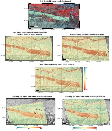
Figure 11.
Normalized aeolian erosion (n-AER) maps using ALOS PALSAR-2 pairs of 2007–2009 (a) and 2015–2017 (b). Two n-AER maps now can be assessed against each other as the data ranges of the two maps used the process of employing control points (see Figure 8a). The effects of activities to combat desertification are evident as presented in circled areas.

Figure 12.
n-AER maps using Sentinel-1 in 2016 (a), 2017 (b), 2018 (c), 2019 (d), and 2020 (e). See the dotted ellipses where n-AER successfully detects the effect of ground compaction around solar panels. Note the range of n-AER is now adjusted between 0.0 to 1.0.
Figure 12.
n-AER maps using Sentinel-1 in 2016 (a), 2017 (b), 2018 (c), 2019 (d), and 2020 (e). See the dotted ellipses where n-AER successfully detects the effect of ground compaction around solar panels. Note the range of n-AER is now adjusted between 0.0 to 1.0.

Figure 13.
n-AER values using Sentinel-1 and PALSAR-1/2 over combat desertification areas (outlined by black dash line in (a)). The performance over all planting areas are shown in (b). Note the effects of combat desertification activities are highly obvious in the observations of very early planting such as 2006–2010 in (c), 2010 in (d) and possibly 2015 (e) employing PALSAR-1 and 2. However, the n-AER changes after 2016 measured by Sentinel-1 observations, such as 2019 (f) and 2020 (g), are not clear.


Table 1.
Employed PALSAR 1 (left part)/2 (right part) InSAR pairs and their acquisition conditions together with spatial phase coherences (Bp: perpendicular baseline (m), Bt: temporal baseline (day), Spatial coh1: spatial phase coherences in mean topographic slope angle (3.34 °). Spatial coh2: spatial phase coherences in mean topographic slope angle (28.3 °). The samples of topographies to calculate Spatial coh1 and 2 were taken from a low sloped plain and high-relief dune field.
| Master Date | Slave Date | Bp | Bt | Spatial Coh1 | Spatial Coh2 | Master Date | Slave Date | Bp | Bt | Spatial Coh1 | Spatial Coh2 |
|---|---|---|---|---|---|---|---|---|---|---|---|
| 11 July 2007 | 26 August 2007 | 251 | 46 | 0.955 | 0.967 | 18 July 2015 | 23 September 2015 | 85 | 70 | 0.985 | 0.987 |
| 26 August 2007 | 11 October 2007 | 389 | 46 | 0.931 | 0.948 | 15 July 2015 | 02 December 2015 | −1.6 | 140 | 1.000 | 1.000 |
| 11 October 2007 | 26 February 2007 | 1209 | 138 | 0.785 | 0.839 | 23 September 2015 | 02 December 2015 | −83 | 70 | 0.985 | 0.988 |
| 26 February 2008 | 12 April 2008 | 437 | 46 | 0.922 | 0.942 | 10 February 2016 | 13 July 2016 | 95 | 154 | 0.983 | 0.986 |
| 26 February 2008 | 28 May 2008 | 274 | 92 | 0.951 | 0.964 | 10 February 2016 | 23 September 2015 | 25 | −140 | 0.995 | 0.996 |
| 12 April 2008 | 28 May 2008 | −163 | 46 | 0.971 | 0.978 | 13 July 2016 | 10 February 2016 | −94.9 | −154 | 0.983 | 0.986 |
| 28 August 2008 | 13 October 2008 | 955 | 46 | 0.830 | 0.873 | 13 July 2016 | 21 September 2016 | 53.9 | 70 | 0.990 | 0.992 |
| - | - | - | - | - | - | 13 July 2016 | 30 November 2016 | −141.8 | 140 | 0.974 | 0.979 |
| - | - | - | - | - | - | 21 September 2016 | 30 November 2016 | −88 | 70 | 0.984 | 0.987 |
| - | - | - | - | - | - | 21 September 2016 | 08 February 2017 | 69.8 | 140 | 0.987 | 0.990 |
| - | - | - | - | - | - | 30 November 2016 | 08 February 2017 | 157.8 | 70 | 0.971 | 0.976 |
Table 2.
Employed Sentinel-1 pairs and their acquisition conditions together with spatial phase coherences (Bp: perpendicular baseline (m), Bt: temporal baseline (day), Spatial coh1: spatial phase coherences in mean topographic slope angle (3.34 °), Spatial coh2: spatial phase coherences in mean topographic slope angle (28.3 °)).
| 2016/2017 | |||||||||||
| Master Date | Slave Date | Bp | Bt | Spatial Coh1 | Spatial Coh2 | Master Date | Slave Date | Bp | Bt | Spatial Coh1 | Spatial Coh2 |
| 16 May 2016 | 09 June 2016 | 17 | 25 | 0.988 | 0.992 | 12 March 2017 | 05 April 2017 | 63 | 24 | 0.954 | 0.968 |
| 09 June 2016 | 03 July 2016 | 7 | 25 | 0.995 | 0.997 | 05 April 2017 | 11 May 2017 | 12 | 36 | 0.991 | 0.994 |
| 03 July 2016 | 20 August 2016 | 3 | 47 | 0.998 | 0.999 | 11 May 2017 | 04 June 2017 | 38 | 24 | 0.972 | 0.981 |
| 20 August 2016 | 07 October 2016 | 49 | 48 | 0.965 | 0.978 | 04 June 2017 | 10 July 2017 | 110 | 36 | 0.919 | 0.944 |
| 25 September 2016 | 07 October 2016 | 75 | 13 | 0.947 | 0.967 | 10 July 2017 | 03 August 2017 | 74 | 24 | 0.945 | 0.963 |
| 07 October 2016 | 12 November 2016 | 111 | 37 | 0.921 | 0.951 | 03 August 2017 | 08 September 2017 | 81 | 37 | 0.940 | 0.959 |
| 12 November 2016 | 06 December 2016 | 35 | 25 | 0.975 | 0.984 | 08 September 2017 | 02 October 2017 | 78 | 24 | 0.943 | 0.961 |
| 06 December 2016 | 11 January 2017 | 179 | 37 | 0.873 | 0.920 | 02 October 2017 | 07 November 2017 | 5 | 48 | 0.996 | 0.997 |
| - | - | - | - | - | - | 07 November 2017 | 01 December 2017 | 52 | 24 | 0.962 | 0.974 |
| 2018/2019 | |||||||||||
| Master Date | Slave Date | Bp | Bt | Spatial Coh1 | Spatial Coh2 | Master Date | Slave Date | Bp | Bt | Spatial Coh1 | Spatial Coh2 |
| 06 January 2018 | 11 February 2018 | 13 | 36 | 0.990 | 0.993 | 02 December 2018 | 01 January 2019 | 26 | 24 | 0.981 | 0.987 |
| 11 February 2018 | 07 March 2018 | 11 | 24 | 0.992 | 0.994 | 01 January 2019 | 06 February 2019 | 5 | 48 | 0.996 | 0.997 |
| 07 March 2018 | 12 April 2018 | 52 | 36 | 0.962 | 0.974 | 06 February 2019 | 02 March 2019 | 143 | 24 | 0.895 | 0.928 |
| 12 April 2018 | 06 May 2018 | 49 | 24 | 0.964 | 0.975 | 02 March 2019 | 07 April 2019 | 28 | 36 | 0.979 | 0.986 |
| 06 May 2018 | 11 June 2018 | 3 | 37 | 0.998 | 0.998 | 07 April 2019 | 01 May 2019 | 64 | 24 | 0.953 | 0.968 |
| 11 June 2018 | 05 July 2018 | 41 | 48 | 0.970 | 0.979 | 01 May 2019 | 06 June 2019 | 83 | 36 | 0.939 | 0.958 |
| 05 July 2018 | 10 August 2018 | 83 | 93 | 0.939 | 0.958 | 06 June 2019 | 12 July 2019 | 27 | 36 | 0.980 | 0.986 |
| 10 August 2018 | 03 September 2018 | 173 | 24 | 0.873 | 0.913 | 12 July 2019 | 05 August 2019 | 34 | 24 | 0.975 | 0.983 |
| 03 September 2018 | 09 October 2018 | 174 | 36 | 0.872 | 0.912 | 05 August 2019 | 10 September 2019 | 45 | 48 | 0.967 | 0.977 |
| 09 October 2018 | 02 November 2018 | 94 | 24 | 0.931 | 0.953 | 10 September 2019 | 04 October 2019 | 104 | 24 | 0.923 | 0.948 |
| - | - | - | - | - | - | 04 October 2019 | 09 November 2019 | 123 | 36 | 0.909 | 0.938 |
| - | - | - | - | - | - | 09 November 2019 | 03 December 2019 | 10 | 24 | 0.993 | 0.995 |
| - | - | - | - | - | - | 03 December 2019 | 08 January 2020 | 79 | 36 | 0.942 | 0.960 |
| 2020 | |||||||||||
| Master Date | Slave Date | Bp | Bt | Spatial Coh1 | Spatial Coh2 | Master Date | Slave Date | Bp | Bt | Spatial Coh1 | Spatial Coh2 |
| 08 January 2020 | 01 February 2020 | 71 | 4 | 0.948 | 0.964 | 18 July 2020 | 11 August 2020 | 116 | 24 | 0.915 | 0.941 |
| 01 February 2020 | 08 March 2020 | 5 | 36 | 0.996 | 0.997 | 11 August 2020 | 04 September 2020 | 148 | 24 | 0.891 | 0.925 |
| 08 March 2020 | 01 April 2020 | 54 | 24 | 0.960 | 0.973 | 04 September 2020 | 10 October 2020 | 99 | 28 | 0.927 | 0.950 |
| 01 April 2020 | 18 July 2020 | 102 | 108 | 0.925 | 0.949 | - | - | - | - | - | - |
Table 3.
The metrics of linear and LMA regression models between the PC and Sentinel-1 AER (R2: coefficient of determination).
Table 3.
The metrics of linear and LMA regression models between the PC and Sentinel-1 AER (R2: coefficient of determination).
| 2016 | Model | R2 | RMSE | 2017 | Model | R2 | RMSE | 2018 | Model | R2 | RMSE |
| Linear | Y = −0.074 × X − 0.822 | 0.024 | 0.079 | Linear | Y = −0.087 × X − 0.737 | 0.023 | 0.072 | Linear | Y = −0.108 × X − 0.668 | 0.056 | 0.074 |
| RMA | Y = −0.469 × X + 0.157 | 0.372 | 0.137 | RMA | Y = −0.567 × X + 0.426 | 0.371 | 0.126 | RMA | Y = −0.458 × X + 0.195 | 0.396 | 0.12 |
| 2019 | Model | R2 | RMSE | 2020 | Model | R2 | RMSE | - | - | - | - |
| Linear | Y = −0.081 × X − 0.796 | 0.027 | 0.088 | Linear | Y = −0.213 × X − 0.421 | 0.152 | 0.084 | - | - | - | - |
| RMA | Y = −0.495 × X + 0.231 | 0.375 | 0.151 | RMA | Y = −0.547 × X + 0.392 | 0.45 | 0.671001 | - | - | - | - |
Table 4.
Distribution of low EVI areas and their n-AER values.
| EVI Threshold (<EVI) | 2007 LANDSAT 5 EVI | 2016 LANDSAT 8 EVI | ||||
| Ratio * in 2007 | Mean n-AER Value in 2007 | n-AER Stdev in 2007 | Ratio in 2016 | Mean n-AER Value in 2016 | n-AER Stdev in 2016 | |
| 0.2 | 99.34 | 0.355 | 0.122 | 81.96 | 0.349 | 0.148 |
| 0.15 | 92.26 | 0.363 | 0.122 | 50.7 | 0.396 | 0.161 |
| 0.1 | 76.88 | 0.377 | 0.126 | 6.56 | 0.6 | 0.095 |
| EVI Threshold (<EVI) | 2007 MODIS EVI | 2016 MODIS EVI | ||||
| Ratio in 2007 | Mean n-AER Value in 2007 | n-AER Stdev in 2007 | Ratio in 2016 | Mean n-AER Value in 2016 | n-AER Stdev in 2016 | |
| 0.2 | 98.48 | 0.356 | 0.122 | 95.2 | 0.337 | 0.144 |
| 0.15 | 87.29 | 0.365 | 0.123 | 80 | 0.348 | 0.15 |
| 0.1 | 43.8 | 0.428 | 0.135 | 30.4 | 0.467 | 0.162 |
* Percentage of the area where EVI value less than EVI threshold.
Publisher’s Note: MDPI stays neutral with regard to jurisdictional claims in published maps and institutional affiliations. |
© 2021 by the authors. Licensee MDPI, Basel, Switzerland. This article is an open access article distributed under the terms and conditions of the Creative Commons Attribution (CC BY) license (https://creativecommons.org/licenses/by/4.0/).
Share and Cite
MDPI and ACS Style
Kim, J.-R.; Lin, C.-W.; Lin, S.-Y. The Use of InSAR Phase Coherence Analyses for the Monitoring of Aeolian Erosion. Remote Sens. 2021, 13, 2240. https://0-doi-org.brum.beds.ac.uk/10.3390/rs13122240
AMA Style
Kim J-R, Lin C-W, Lin S-Y. The Use of InSAR Phase Coherence Analyses for the Monitoring of Aeolian Erosion. Remote Sensing. 2021; 13(12):2240. https://0-doi-org.brum.beds.ac.uk/10.3390/rs13122240
Chicago/Turabian StyleKim, Jung-Rack, Cheng-Wei Lin, and Shih-Yuan Lin. 2021. "The Use of InSAR Phase Coherence Analyses for the Monitoring of Aeolian Erosion" Remote Sensing 13, no. 12: 2240. https://0-doi-org.brum.beds.ac.uk/10.3390/rs13122240
Note that from the first issue of 2016, this journal uses article numbers instead of page numbers. See further details here.