
Statistically-Based Trend Analysis of MTInSAR Displacement Time Series


National Research Council of Italy, Institute for Electromagnetic Sensing of the Environment (IREA), Via Amendola, 122/d, 70126 Bari, Italy
*
Author to whom correspondence should be addressed.
Remote Sens. 2021, 13(12), 2302; https://0-doi-org.brum.beds.ac.uk/10.3390/rs13122302
Submission received: 19 May 2021
/
Revised: 8 June 2021
/
Accepted: 10 June 2021
/
Published: 11 June 2021
(This article belongs to the Special Issue SAR Interferometry: Methods and Applications for Earth Science and Environmental Monitoring)
Abstract
:Current multi-temporal interferometric Synthetic Aperture Radar (MTInSAR) datasets cover long time periods with regular temporal sampling. This allows high-rate and non-linear trends to be observed, which typically characterize pre-failure warning signals. In order to fully exploit the content of MTInSAR products, methods are needed for the automatic identification of relevant changes along displacement time series and the classification of the targets on the ground according to their kinematic regime. This work reviews some of the classical procedures for model ranking, based on statistical indices, which are applied to the characterization of MTInSAR displacement time series, and introduces a new quality index based on the Fisher distribution. Then, we propose a procedure to recognize automatically the minimum number of parameters needed to model a given time series reliably within a predefined confidence level. The method, though general, is explored here for polynomial models, which can be used in particular to approximate satisfactorily and with computational efficiency the piecewise linear trends that are generally used to model warning signals preceding the failure of natural and artificial structures. The algorithm performance is evaluated under simulated scenarios. Finally, the proposed procedure is also demonstrated on displacement time series derived by the processing of Sentinel-1 data.
1. Introduction
Multi-temporal SAR interferometry (MTInSAR) techniques have been used for the last two decades to derive displacement maps and displacement time series over coherent objects on the Earth and thus to monitor geophysical ground deformations or infrastructural instabilities [1,2]. Several datasets are currently available at different wavelengths, spatial resolutions, and revisit times, spanning national [3,4,5] or continental [6] areas, and collectively covering long time periods (even more than 20 years). In particular, the short revisit times (e.g., from the European Sentinel-1 and the Italian COSMO-SkyMed constellations) achieved by improving the temporal sampling make it theoretically possible to catch the high-rate and non-linear kinematics that typically characterize warning signals related to, for instance, landslides or the pre-failure of artificial infrastructures.
Despite the early recognition of the importance of nonlinear analysis [7], displacement signals in MTInSAR time series are still often treated by using a linear model, which is computationally convenient and also more robust than higher-order models with regard to the errors affecting the InSAR phase. In fact, the spatial analysis of MTInSAR products is often performed by only considering the mean displacement rate, computed over the entire monitoring period, which is the information typically displayed on displacement maps.
To fully exploit the content of MTInSAR products, methods are needed to automatically identify relevant changes in displacement time series and to classify the targets on the ground according to their kinematic regime. This would also allow a more reliable ground deformation spatial analysis to be conducted by distinguishing between spatial patterns of different types (linear, bi-linear, quadratic, discontinuous, periodic, etc.).
Recently, approaches have been proposed to tackle this problem that use different strategies based, e.g., on Principal Component Analysis [8], statistical tests [9], or more sophisticated probabilistic multiple hypothesis testing [10]. Mostly, these approaches consider a finite number of models and use statistical methods to discriminate the model that best fits each time series. Many works add a subsequent spatial analysis to better define areas that are subject to homogeneous displacement regimes. This mainly stems from the fact that assigning a certain displacement model to a single time series independently of any other information is extremely difficult for MTInSAR data. This is due to several factors, such as the presence of noise coming from the incomplete removal of signal components such as atmospheric artifacts or topographic errors, which reduces the identification performance, and also the intrinsic requirements of MTInSAR algorithms, which must postulate some form of regularity in time to identify stable scatterers in the first place. This regularity constraint is in most cases implemented in a linear manner, or through a limited library of simple models, and such assumptions may “leak” into the posterior modeling operations.
Maintaining independence among individual stable target MTInSAR time series has some advantages, especially in applications with complex environments such as urbanized areas, where—at least with the current SAR sensor resolutions that reach at most a few meters—deformation processes, causes, and models can vary drastically from pixel to pixel. In this sense, in [11], a method is proposed to characterize the regularity of each individual time series independently and without any assumption of the displacement model. Based on the index known as Fuzzy Entropy, the method identifies, with good efficiency, time series characterized by low noise and temporal regularity for at least a part of their length.
However, discriminating among a library of different parametric kinematic models remains a useful objective, as often recognizing abrupt discontinuities [12] or the triggering of nonlinear trends [13], for example, may allow researchers to efficiently monitor vast areas for various hazards. Although these considerations are in principle applicable to any parametric function, we focus here on the application to polynomials, which allow a large class of different temporal trends to be modeled. In fact, polynomial fits can be used, e.g., to reliably discern nonlinear trends (degree > 1) from linear trends. They can also accommodate various types of discontinuities, such as impulsive changes of linear rates (e.g., first-order discontinuities, or piecewise linear trends), with the advantage of avoiding the determination of critical parameters such as the position of the discontinuities on the time axis, which is not easy and requires considerable computational resources [14,15].
Some classical indices have traditionally been used to score the goodness of fit of parametric models according to confidence intervals [16], or more generally to rank different models [17,18] by taking into account the obvious increase of fitting performances due to the increase of the number of model parameters. These indices seem to have been rarely used [9] in applications involving MTInSAR data.
In this article, we study the reliability of such classical tests—namely the Fisher test [16], the Akaike Information Criterion [17], and the Bayesian Information Criterion [18]—for comparing different polynomial models. We then introduce a new statistical test based on the Fisher distribution with the aim of evaluating the reliability of a parametric displacement model fit with a determined statistical confidence. We also propose a new set of rules based on the statistical characterization of displacement time series, which allows, under certain constraints, different polynomial approximations for MTInSAR time series to be ranked, and thus allows the minimum set of relevant parameters useful for target characterization to be estimated.
Our performance analysis is carried out by simulating time series with piecewise linear temporal trends, with different breakpoints and velocities, levels of noise, signal lengths, and temporal sampling. In fact, piecewise linear trends are another rather general type of model that may be chosen to interpret several phenomena of incipient displacements; e.g., for landslides or infrastructures such as dams or bridge pillars. As mentioned, velocity breaks can be approximated by polynomial trends with a degree >1, and thus a method to reliably detect the most appropriate minimum polynomial degree approximating a time series can be used to isolate “problematic” targets.
Finally, we illustrate the method performance over a selected set of real data derived from the Sentinel-1 SAR constellation.
2. Problem Formulation
Suppose a MTInSAR time series composed by estimations of the displacement signal sampled at time :
where is the noise affecting the MTInSAR estimation, which depends both on the intrinsic scattering characteristics of the target and the processing reliability. In all the following considerations, we refer to the time series as the scalar displacement, with real values (e.g., in mm) projected on the line of sight (LOS), as retrieved by a generic MTI processing chain. By assuming that the MTInSAR processing is able to remove all the other components of the InSAR phase signal (e.g., atmospheric artifacts, orbital errors) [2], the noise can be modeled as Gaussian, with standard deviation and zero mean, and can be assumed not to be correlated with the displacement signal: .
The reliability of a target can be evaluated through a quality index calculated from the difference between the time series values and the value predicted by a displacement model. The most used index in MTInSAR applications is the so-called temporal coherence , defined as [19]
where is the standard deviation of the InSAR phase noise: , where is the radar wavelength.
The temporal coherence is model-dependent: if the adopted displacement model is well suited, the temporal coherence is only related to the phase noise affecting the target () [19], and consequently a good-quality target shows a coherence value close to 1, while for noisy targets, the coherence values decrease toward 0. This is no longer true if the adopted model departs from the actual, “true” displacements: in this case, low coherence values could also occur for pixel time series affected by a small Gaussian noise component, but a larger difference could be found between modeled and “true” displacements, thus leading to a failure in the detection of such persistent targets.
High coherence values thus ensure that the target has a low intrinsic noise and its displacement is well approximated by the adopted model. In fact, the selection of pixels corresponding to coherent targets (CT) is performed according to :
where are the pixel coordinates, and is a threshold value that can be computed according to the processing settings [19,20]. Although some recent MTInSAR implementations achieve the modeling of non-linear displacement trends by using polynomial and/or periodic functions (e.g., [21,22]), very often, the linear displacement model is used, at least for automatic large-scale processing, in order to save computational time. This means that, in case a non-linear displacement occurs, the estimation of the target noise content through the temporal coherence is biased and, in order to identify targets showing non-linear displacement trends, pixels with low coherent values should also be considered.
This work aims to develop a set of rules based on both state-of-the-art and innovative indices to identify the model which best approximates the displacement trend of MTInSAR time series. The ideal selection process should allow the identification of non-linearities and for comparisons to be performed between models; furthermore, it should be robust against overfitting (unlike ) and also computationally efficient.
We focus here on polynomial models, and so our goal is to approximate the displacement time series with a polynomial with degree :
As mentioned above, polynomial models can be used to successfully approximate a large class of ground displacement regimes. For instance, polynomial degrees >1 generally characterize discontinuous trends such as instantaneous velocity breaks, so targets requiring polynomial approximations with a degree >1 are immediately worthy of attention. More complex types of trends can also be approximated by polynomials, such as impulsive displacements or creeping.
Several standard absolute indices can be used to estimate the deviation between data and a model function; e.g., the mean error (ME), mean square error (MSE), root mean square error (RMSE), and the coefficient of determination , which can be defined as follows [23]:
The choice of the best model should also take into account the number of degrees of freedom of the problem, which in the case of a polynomial function is the polynomial degree, . In fact, as is well known, the higher the degree used in a fit (or, more generally, the number of parameters), the smaller the deviation of the model from the measured data. In the literature, several methods exist to compare different models by also taking into account their degrees of freedom; e.g., the F test, [16], Akaike’s Information Criterion (AIC) [17], and the Bayesian Information Criterion (BIC) [18].
2.1. F Test
Suppose two polynomials models are defined by (4) with degrees ; then, the F test statistic is defined as follows ([24] pp. 138–142):
This indicator follows the Fisher–Snedecor distribution [16,25] , , and allows the two models to be compared by testing the null hypothesis H0; i.e., that the difference of the residuals between the measured and approximated data using the two polynomials is not significant. In more detail, the null hypothesis is not rejected with a level of significance if
On the contrary, if , then the null hypothesis is rejected, meaning that the displacement trend modeled by the polynomial of higher degree is significantly different than that obtained by the polynomial , with a significance equal to or, equivalently, with a confidence level equal to . is the quantile of order relative to the Fisher distribution, which can be calculated as a function of and [25] (pp. 102–106). The curves in Figure 1 correspond to and a confidence level ranging between 0.90 and 0.99, and these can be used to set in (6). For instance, assuming two nested polynomial models ( with a number of samples , the value corresponding to confidence level 0.95 is roughly 4. If H0 is not satisfied by a certain degree n, we could therefore increase by 1 the degree and perform the test again, until the condition is reached in which an additional degree does not violate the H0 hypothesis, which would correspond to the sought minimum degree.
2.2. Akaike Information Criterion (AIC) and Bayesian Information Criterion (BIC)
The Akaike Information Criterion (AIC) [17] is widely used in non-linear regression problems. This selection criterion is based on the Kullback–Leibler information loss that occurs when data are approximated by a model. The value of the AIC index in the case of a model with parameters and data is calculated as follows [26]:
where the last term is needed only if in order to avoid a bias in the estimation.
Since AIC is related to the information loss, the best model will be the one that minimizes this loss. Therefore, supposing we have M polynomial models , the best polynomial will be that with the minimum AIC value: . Moreover, since the AIC is used to compare different models, AIC values are usually referred to this minimum value by defining the quantity .
A reliable selection should assess whether the difference between two models actually involves a significant loss of information or whether they could be considered equivalent. Rules of thumb for evaluating the significance of the difference between two models are provided in [26], and are reported as follows:
- : both models have substantial support;
- : has considerably less support than ;
- : has no support.
Another criterion used in the literature (e.g., [9]) is the Bayesian Information Criterion (BIC). It is related to the AIC and can be defined as follows [18]:
The BIC index, similarly to the AIC, compares two models and allows the model with the lowest value to be selected; thus, in this case, the differential value is also computed: , where is the model providing the minimum BIC value. Compared to the AIC, the BIC has an additional penalty factor proportional to the number of parameters. In [26], an extensive discussion is presented concerning the reliability of the BIC and AIC indices, and their performances are analyzed in several applicative test cases. In general, the performance of the BIC improves as increases, but no relevant differences are reported between the BIC and AIC. However, unlike for the AIC, there are no rigorous rules for assessing the significance of the difference between BIC values that can be adopted in the process of model selection. This could represent a critical issue in case the BIC is adopted for automatic selection procedures. According to this, the BIC index was excluded from the following performance analysis.
2.3. Index
The indices introduced so far are either absolute measures of a model’s adequacy () but not robust with respect to the noise affecting the time series, or comparative figures, designed to select the best among several models but without assigning a statistical reliability value to that choice. In order to overcome these limitations, a new index is proposed here that is able to estimate the degree to which a polynomial is representative of a data trend and to associate a statistically based degree of significance to this estimate. The robustness of the index is pursued by decoupling the noise affecting the data series from the contribution related to the difference between the actual data trend and the model chosen to approximate the data.
Referring to the displacement time series signal defined by (1), the basic idea is to find a way to evaluate the difference between the true deformation, , and the polynomial defined by (4), and to approximate this signal by avoiding the effect of the noise affecting the data. All the absolute indices introduced above depend on the differences (residuals) between the input and model values ( and thus are related, explicitly or implicitly, to the standard deviation of the noise, .
The aim of the index is to statistically estimate whether these differences are due to noise or to an unreliable polynomial approximation. This is accomplished by comparing the mean squared sum of the differences, , divided by the noise variance , and the squared difference between the means, , divided by the variance affecting the mean, . These two ratios compare the squared difference between the signal and model (and between their means) with respect to the noise variance, thus somehow estimating the percentage of difference between the signal and model that can be explained in terms of noise. Moreover, these ratios are distributed according to the chi-square distribution with and one degree of freedom, respectively. The index is thus defined by dividing these two normalized ratios by their degrees of freedom:
This index has several advantages with respect to the indices introduced before. First, does not depend on , and thus allows the reliability with which the polynomial model approximates the deterministic trend of the data to be estimated, regardless of the contribution of the noise. This is a crucial point since the performances of the previous indices are strongly biased due to noise. Furthermore, as it is derived by the ratio of chi-squared distributed variances, follows the Fisher statistics: . This latter aspect is important because it allows the index to be used to test the reliability of the polynomial model and to quantify the test significance statistically, in the same way as shown in Section 2.1 for the index. In more detail, the null hypothesis ()—that the model is representative of the data—is not rejected with a level of significance if
On the contrary, if , then the representation of the displacements obtained with the polynomial of degree must be rejected with a significance equal to or equivalently with a confidence level equal to . As for , is the quantile of order relative to the Fisher distribution, which can be calculated as a function of and . The numerical values are the same as those computed for and reported in Figure 1: assuming , the value corresponding to a confidence level of 0.95 is about 4.
3. Performance Analysis
In order to compare the reliability of the indices introduced so far, a performance analysis is carried out by using simulated displacement time series. The simulations are set according to the following input parameters: the number of samples of the time series (), the sampling time interval (dt), the wavelength (), the temporal coherence (), which defines the noise level according to Equation (2), and the displacement kinematic model. In particular, a piecewise kinematic model was adopted, constructed with two linear trends with velocities and and a transition at time .
For each simulated time series, a least squares fit is performed by using a polynomial model defined by (4), with the degrees increasing from 1 to 4. Then, the polynomial model most representative of the simulated time series is selected by adopting as a quality figure both the absolute () and relative () proposed indices. The value is computed through (5) with , thus allowing the comparison between polynomials of consecutive degrees.
An example of a simulation is reported in Figure 2a, showing a piecewise linear displacement signal of 100 samples at a constant time interval of 6 days, which is relevant to the case of the European Space Agency (ESA)’s Sentinel-1—the current SAR sensor constellation with the highest revisit frequency and thus the best candidate to provide long time series that are able to detect non-linear ground displacement. Figure 2b shows the polynomial analysis of the time series in (a), and the legend panel reports the values of the quality indices computed for each polynomial model. In this particular case, we highlight the and values, which fall below the 4 threshold for degrees ≥2, thus indicating the parabolic trend to be the most appropriate (minimum degree). This is confirmed by the polynomial curve trends of order 2 to 4, which appear largely superposed.
The performance analysis is carried out by running the simulation scheme described above to compute the index values corresponding to different settings of the input parameters; namely, , and (corresponding to ). Table 1 reports the values of the input parameters explored to assess the reliability of the indices in selecting the best polynomial model. Wherever units are not specified, the parameter is considered adimensional. This work is focused in particular on warning signals related to the pre-failure of natural or artificial structures, which typically show quite high displacement rate values; in particular, during the accelerated phase preceding the failure (e.g., [27,28]). For instance, typical threshold values used to classify a slope as active and susceptible to failure are in the order of 2 cm/year [29,30]. According to this, in our simulations, we explore displacement rate values in the order of centimeters per year.
For each parameter configuration and for each degree of the polynomial model used to fit the time series in the input, we derived the corresponding set of indices and polynomial coefficients . In order to deal with the random nature of the noise, for each parameter configuration, both index and coefficient values are computed by averaging the results corresponding to input signals, obtained by combining the same deterministic displacement trend with different realizations of a Gaussian noise with zero mean and standard deviation . According to this simulation scheme, and are computed for all configurations in Table 1. As stated in Section 2.2, the AIC is normalized with respect to the minimum value by computing the ΔAIC.
In order to analyze the simulation results, we plot the index trends as a function of the simulated velocity change in the time series, , computed for different values of noise level and transition time . An example is reported Figure 3, which shows in each plot the trends of , and ΔAIC as a function of in cm/year, computed for ranging from 1 to 4 (corresponding to different line styles as detailed in the title). The plots along each row refer to different noise levels, decreasing as ranges from 0.5 to 0.9. All the simulated time series have a fixed transition time that occurs at half the timespan ( = T/2). As the velocity difference increases (from 0 to 5 cm/year), the simulated displacement trend increasingly deviates from linearity, and thus the polynomial order needed to approximate the trend should also increase. According to this, the expected trend of the index values is that increasingly high minimum polynomial degrees should be selected as increases; indeed, this is basically what the plots show when comparing the index trends corresponding to different values of . Moreover, the plots show different index change rates as changes, as well as different sensitivities to the noise level. For instance, ΔAIC trends show considerable variations compared to the other indices, while both and show fairly similar trends for different noise levels. Similar behaviors have been observed by simulating displacement trends with different transition times (up to ), which are not shown for brevity.
The performance analysis is carried out by using each of the six indices to select the minimum polynomial model that is representative of the displacement time series in the input: . To this end, we adopt the following selection rules, some of which were introduced in the previous sections and are listed again here for convenience:
- ;
- ;
- ;
- ;
- ;
- .
The threshold values and are derived from Figure 1 according to a confidence level 0.95 and a number of samples of the simulated time series of = 100.
These selection rules were used to process the time series generated by exploring all the configurations that can be derived from Table 1. The polynomial degrees selected according to these rules are then analyzed as a function of the velocity change , the transition time , and the noise level defined by . An example is reported in Figure 4, where each plot shows, as a function of in cm/year, the trends of the polynomial degree selected by using , and ΔAIC, from the top to bottom row of the figure, respectively. As in Figure 3, the plots along each row refer to decreasing noise levels, with ranging from 0.5 to 0.9, and are derived by simulating time series with a transition time . The missing values in the plots correspond to configurations for which no polynomial model fulfills the selection rules.
The ideal index should be able to select the most reliable polynomial model for any value of the nonlinearity degree defined by the velocity change and of the noise level of the input signal. In particular, as the velocity difference increases, the polynomial degree needed to approximate the simulated displacement trend should also increase. Moreover, the index should also be able to catch small velocity changes in order to reliably detect weak precursory displacement signals.
By inspecting the plots in Figure 4, we can conclude that indices , and are neither robust against noise nor able to detect small velocity changes. On the contrary, indices , , and ΔAIC provide a reliable polynomial selection for any velocity change and noise level. In particular, the performances of and ΔAIC are very similar for all the explored configurations; these indices are able to select the polynomial that most likely best approximates the simulated displacement time series.
4. Results and Discussion
The performance analysis presented in the previous section allows the index reliability to be assessed and for us to set definite rules for selecting the polynomial model that best approximates a MTInSAR displacement time series. The analysis indicates that and are the most reliable indices, which show similar performances. However, there is no rigorous criterion for setting the threshold value for (), while follows the well-known Fisher statistics, and thus the threshold value can be computed according to the number of samples () and a required confidence level (p). Thus, appears to be the most suitable index for the polynomial selection. However, it is a relative index and thus only allows the best between two different models to be selected, without providing any estimation of the absolute significance of the result. To this end, the index can be used, which is instead able to estimate the absolute reliability of a polynomial model of degree and is robust against noise. Moreover, even in this case, it is possible to set the threshold value rigorously according to the number of samples and to a required confidence level. Therefore, the final selection rule is defined by coupling and as follows:
Figure 5 shows the processing scheme proposed for the analysis of the MTInSAR displacement time series. The input data are time series derived by a generic MTInSAR algorithm and characterized by temporal coherence () computed according to the displacement model adopted by the algorithm. The outputs of the proposed analysis are the coefficients of the polynomial model selected for describing the time series (4); the proposed Fisher index , which allows the quality of the approximation provided by the selected polynomial model to be evaluated; and the temporal coherence , computed with (2) by using the selected polynomial model.
The output coherence should improve the estimation of the residual noise with respect to the level provided by , which is assumed to be computed using a linear model (as often occurs in MTInSAR processing, at least for large-scale processing). Therefore, a new and more reliable set of coherent targets can be derived through (3) by using .
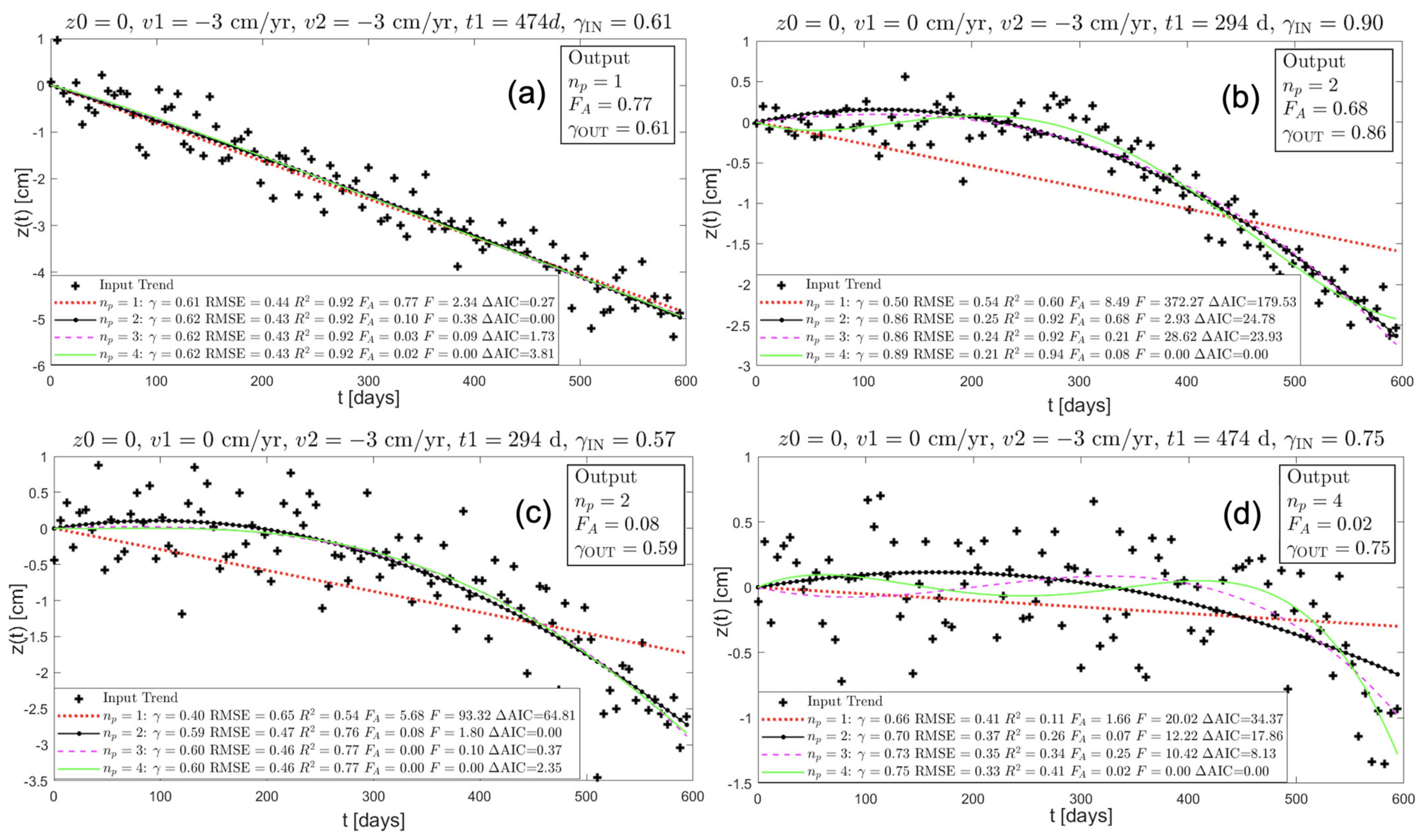
Figure 6 shows four examples of simulated time series of 100 samples each, at a time spacing of 6 days, analyzed with the proposed method. The plot in (a) refers to a relatively noisy linear trend. In this simple case, all the indices are able to select the polynomial model of the first degree. Time series in (b) and (c) consist of piecewise linear trends with velocities = 0 and = −3 cm/year, a transition time , and noise levels corresponding to temporal coherences of 0.9 (low noise) and 0.57 (strong noise), respectively. On the contrary, the temporal coherence, being strongly biased by the noise, would have failed to select the reliable model in the noisy case (c): the value of 0.59 is lower than the threshold (as defined in Section 3). The last plot in (d) refers to a piecewise linear trend with velocities = 0 and = −3 cm/year, and a transition time , which requires a polynomial of higher order to be properly modeled. The proposed method selects a fourth-degree polynomial. The relatively high noise content causes a bias in the temporal coherence, which once again causes a failure to select the proper polynomial model.
Results from Real Data
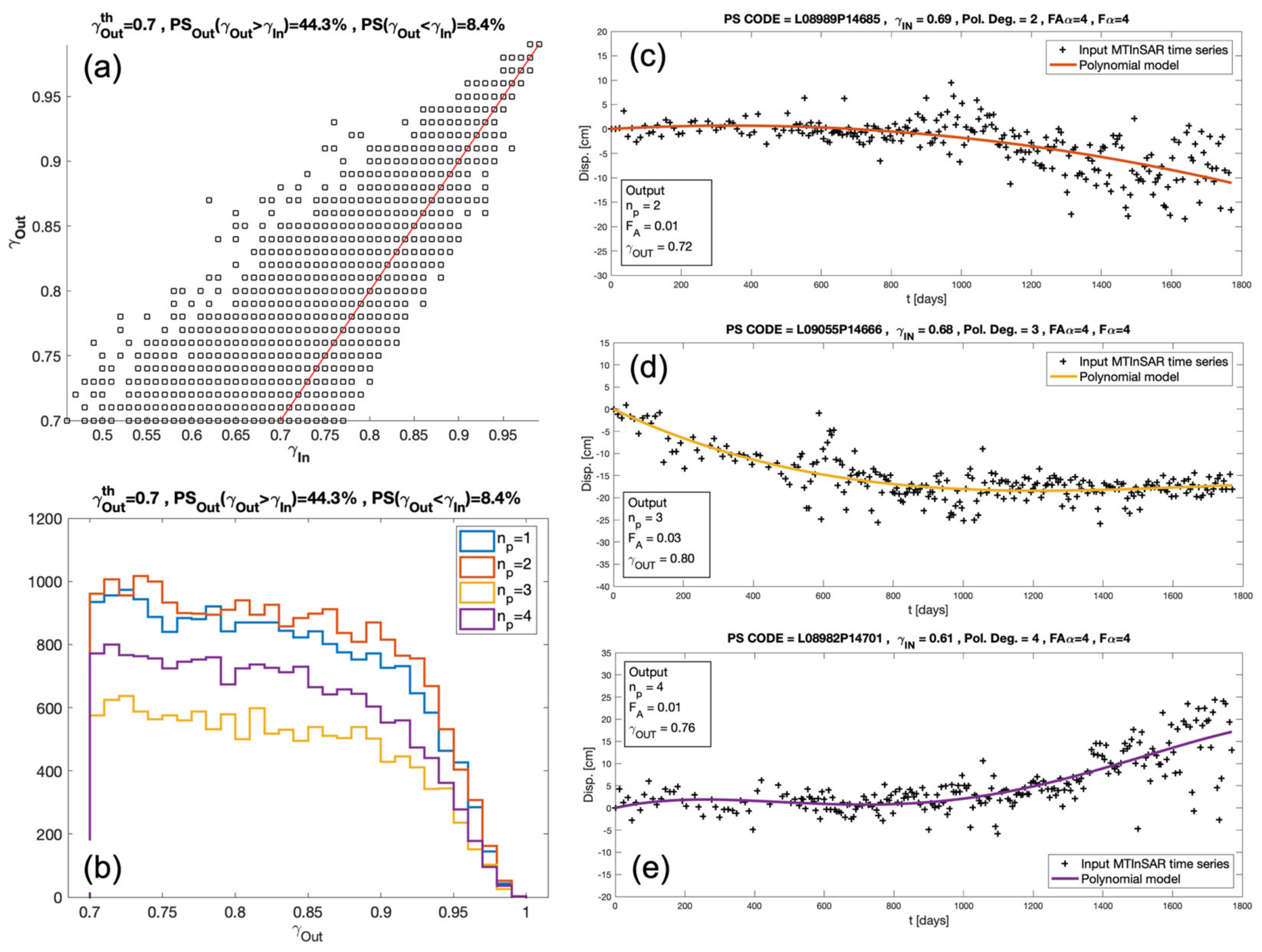
The proposed trend analysis has been run on displacement time series derived by processing real data though a persistent scatterer MTInSAR algorithm [20]. The dataset consists of 245 Sentinel-1 SAR images acquired over an urban area between April 2015 and February 2020. The temporal coherence in the input is computed by adopting a linear displacement model. According to the number of images, and assuming a confidence level of 0.95, the threshold values used for performing the test (11) are .
The values are then used for the CT selection through (3) with = 0.7, resulting in a number of pixels . By comparing this CT set with that derived by using the , we measure an increase of the CT number of about 5.3%. This demonstrates that the proposed trend analysis actually improves the modeling of displacement trends, which in turn leads to an increase in the temporal coherence values. This is clearly visible in Figure 7a, showing the scatterplot of versus : 44.3% of the CTs lay above the main diagonal (red line), meaning that they have . Figure 7b shows the distributions corresponding to polynomial degrees ranging from 1 (linear) to 4, while plots (c), (d), and (e) show examples of nonlinear displacement time series selected according to the output of the proposed trend analysis. The continuous colored lines represent the polynomial functions modeling the MTInSAR displacement values in the input (black crosses). In all cases, the values are below the threshold, thus meaning that these pixels are not selected as CTs in the linear case. The proposed trend analysis was instead able to derive more reliable displacement models that increase the values above the threshold and allow the pixels to be classified as CT.
The proposed procedure can also be used to simplify the analysis of MTInSAR products as it allows the selection of a smaller set of CTs according to a particular displacement kinematic of interest. For instance, if we were interested in analyzing only nonstationary displacement trends, which are interesting for geophysical and geotechnical investigations, by using the original MTInSAR product, we would set a low coherence threshold (e.g., ) to include possible nonlinear trends. This means selecting about 38% of the image pixels, including those strongly affected by noise. On the contrary, by using the products derived from the trend analysis, we are able to select only CTs showing non-linear displacement (), which are about 62% less in number than those selected by using . The analysis of this smaller set of targets to properly interpret their displacement time series is more manageable than analyzing the whole data set. This kind of advantage is expected to be increasingly important as huge quantities of MTInSAR products at a national or continental scale become available [31,32,33].
5. Conclusions
The present work tackles the problem of automatically classifying MTInSAR displacement time series to identify those showing non-linear kinematics. In particular, it focuses on the problem of reliably assigning a minimum degree to a polynomial approximation of each time series, thus automatically detecting nonlinearities (as polynomials with a degree >1) such as piecewiselinear trends, which are typical of warning signals preceding the failure of natural and artificial structures.
We introduced a new statistical test , based on the Fisher distribution, and aimed to evaluate the reliability with which a polynomial model approximates a given trend. We also considered other indices that are commonly used either for comparing different models (F test, the AIC, and the BIC) or for evaluating the residuals between a model and input signal ().
A performance analysis including all these indices has been carried out by simulating piecewise linear time series with different breakpoints, velocities, levels of noise, and signal lengths. Based on this analysis, we proposed a procedure for selecting the polynomial model, which involves computing the and statistics and comparing them to threshold values that can be set rigorously, according to the number of signal samples, to reach a required statistical confidence level.
The proposed methodology was also illustrated on a real InSAR displacement time series dataset from the Sentinel-1 constellation, which, by providing datasets covering long time periods with a regular and short temporal sampling, is well suited for detecting warning signals related to ground instabilities. The procedure was able to classify the time series according to the polynomial order (from 1 to 4) selected to model the displacement trends. This allows a focus to be placed on the geophysical or geotechnical analysis of the MTInSAR products on a smaller set of coherent targets, which are selected according to the displacement kinematic model of interest. The dataset was obtained by using a linear model to identify the stable targets in the first place—a procedure common to many state-of-the-art algorithms, especially when used for large-scale processing—and we adopted a low threshold on the input temporal coherence to keep nonlinear trends. The proposed post-processing procedure, by adaptively identifying the most appropriate polynomial approximation model, led to an increase in the (output) MTInSAR temporal coherence values, thus allowing a more reliable selection of coherent targets, whether linear or nonlinear. Finally, the computational cost of the proposed procedure is low.
This polynomial analysis could be preceded or followed by other specific processing steps aimed at deriving further parameters to classify nonlinear trends, such as the exact time corresponding to a breakpoint [9] or the predicted failure time for landslides [29]. Furthermore, it can be coupled with other procedures tailored to pick targets with temporal trends affected by a periodic signal, such as those caused by structural thermal oscillations [34] or seasonal ground subsidence [8,10], temporal trends different from any “canonical” displacement trend model, or finally, temporal trends showing a partially coherent behavior in time [11]. These interesting developments are the subject of ongoing research.
Author Contributions
Conceptualization, F.B. and G.P.; methodology, F.B. and G.P.; software, F.B.; validation, F.B., A.R. and G.P.; writing—original draft preparation, F.B. and A.R.; writing—review and editing, F.B., A.R. and G.P. All authors have read and agreed to the published version of the manuscript.
Funding
This work was supported in part by the Italian Ministry of Education, University and Research, D.D. 2261 del 6.9.2018, Programma Operativo Nazionale Ricerca e Innovazione (PON R&I) 2014–2020 under Project OT4CLIMA; and in part by Regione Puglia, POR Puglia FESR-FSE204-2020—Asse I—Azione 1.6 under Project DECiSION (p.n. BQS5153).
Acknowledgments
The authors thank GAP srl and Planetek Italia srl for providing MTInSAR time series through the Rheticus® platform. The Sentinel-1 data were provided through the Copernicus Program of the European Union. Finally, the authors thank M. Mottola for her support.
Conflicts of Interest
The authors declare no conflict of interest.
References
- Crosetto, M.; Monserrat, O.; Cuevas-González, M.; Devanthéry, N.; Crippa, B. Persistent Scatterer Interferometry: A review. ISPRS J. Photogramm. Remote Sens. 2015, 115, 78–89. [Google Scholar] [CrossRef] [Green Version]
- Ho Tong Minh, D.; Hanssen, R.; Rocca, F. Radar Interferometry: 20 Years of Development in Time Series Techniques and Future Perspectives. Remote Sens. 2020, 12, 1364. [Google Scholar] [CrossRef]
- Caro Cuenca, M.; Hanssen, R.F.; Hooper, A.J.; Arikan, M. Surface deformation of the whole Netherlands after PSI analysis. In Proceedings of the Fringe 2011 Workshop, Frascati, Italy, 19–23 September 2011; pp. 1–27. [Google Scholar]
- Costantini, M.; Ferretti, A.; Minati, F.; Falco, S.; Trillo, F.; Colombo, D.; Novali, F.; Malvarosa, F.; Mammone, C.; Vecchioli, F.; et al. Analysis of surface deformations over the whole Italian territory by interferometric processing of ERS, Envisat and COSMO-SkyMed radar data. Remote Sens. Environ. 2017, 202, 250–275. [Google Scholar] [CrossRef]
- Dehls, J.F.; Larsen, Y.; Marinkovic, P.; Lauknes, T.R.; Stodle, D.; Moldestad, D.A. INSAR.No: A National Insar Deformation Mapping/Monitoring Service in Norway—From Concept To Operations. In Proceedings of the IGARSS 2019—2019 IEEE International Geoscience and Remote Sensing Symposium, Yokohama, Japan, 28 July–2 August 2019; pp. 5461–5464. [Google Scholar]
- EU-GMS Task Force. European Ground Motion Service (EU-GMS). A Proposed Copernicus Service Element. 2017. Available online: https://land.copernicus.eu/user-corner/technical-library/egms-white-paper (accessed on 11 June 2021).
- Ferretti, A.; Prati, C.; Rocca, F. Nonlinear subsidence rate estimation using permanent scatterers in differential SAR interferometry. IEEE Trans. Geosci. Remote Sens. 2000, 38, 2202–2212. [Google Scholar] [CrossRef] [Green Version]
- Cohen-Waeber, J.; Bürgmann, R.; Chaussard, E.; Giannico, C.; Ferretti, A. Spatiotemporal Patterns of Precipitation-Modulated Landslide Deformation From Independent Component Analysis of InSAR Time Series. Geophys. Res. Lett. 2018, 45, 1878–1887. [Google Scholar] [CrossRef]
- Berti, M.; Corsini, A.; Franceschini, S.; Iannacone, J.P. Automated classification of Persistent Scatterers Interferometry time series. Nat. Hazards Earth Syst. Sci. 2013, 13, 1945–1958. [Google Scholar] [CrossRef] [Green Version]
- Chang, L.; Hanssen, R.F. A Probabilistic Approach for InSAR Time-Series Postprocessing. IEEE Trans. Geosci. Remote Sens. 2016, 54, 421–430. [Google Scholar] [CrossRef] [Green Version]
- Refice, A.; Pasquariello, G.; Bovenga, F. Model-Free Characterization of SAR MTI Time Series. IEEE Geosci. Remote Sens. Lett. 2020, 1–5. [Google Scholar] [CrossRef]
- Aminikhanghahi, S.; Cook, D.J. A survey of methods for time series change point detection. Knowl. Inf. Syst. 2017, 51, 339–367. [Google Scholar] [CrossRef] [Green Version]
- Hussain, E.; Novellino, A.; Jordan, C.; Bateson, L. Offline-Online Change Detection for Sentinel-1 InSAR Time Series. Remote Sens. 2021, 13, 1656. [Google Scholar] [CrossRef]
- Muggeo, V.M.R. Estimating regression models with unknown break-points. Stat. Med. 2003, 22, 3055–3071. [Google Scholar] [CrossRef]
- Lee, T.S. Change-point problems: Bibliography and review. J. Stat. Theory Pract. 2010. [Google Scholar] [CrossRef]
- Fisher, R.R.A. Statistical Methods for Research Workers; Oliver & Boyd: Edinburgh, UK, 1932; ISBN 0050021702. [Google Scholar]
- Akaike, H. A new look at the statistical model identification. IEEE Trans. Automat. Contr. 1974, 19, 716–723. [Google Scholar] [CrossRef]
- Schwarz, G. Estimating the Dimension of a Model. Ann. Stat. 1978, 6, 461–464. [Google Scholar] [CrossRef]
- Colesanti, C.; Ferretti, A.; Novali, F.; Prati, C.; Rocca, F. SAR monitoring of progressive and seasonal ground deformation using the permanent scatterers technique. IEEE Trans. Geosci. Remote Sens. 2003, 41, 1685–1701. [Google Scholar] [CrossRef] [Green Version]
- Bovenga, F.; Nutricato, R.; Refice, A.; Guerriero, L.; Chiaradia, M.T. SPINUA: A flexible processing chain for ERS/ENVISAT long term interferometry. In Proceedings of the 2004 Envisat & ERS Symposium, Salzburg, Austria, 6–10 September 2004; pp. 473–478. [Google Scholar]
- Crosetto, M.; Monserrat, O.; Cuevas-González, M.; Devanthéry, N.; Luzi, G.; Crippa, B. Measuring thermal expansion using X-band persistent scatterer interferometry. ISPRS J. Photogramm. Remote Sens. 2015, 100, 84–91. [Google Scholar] [CrossRef] [Green Version]
- Morishita, Y.; Hanssen, R.F. Deformation Parameter Estimation in Low Coherence Areas Using a Multisatellite InSAR Approach. IEEE Trans. Geosci. Remote Sens. 2015, 53, 4275–4283. [Google Scholar] [CrossRef]
- Draper, N.R.; Smith, H. Applied Regression Analysis; Wiley Series in Probability and Statistics; John Wiley & Sons, Inc.: New York, NY, USA, 1998; ISBN 9780471170822. [Google Scholar]
- Motulsky, H.; Christopoulos, A. Fitting Models to Biological Data Using Linear and Nonlinear Regression. A Practical Guide to Curve Fitting; GraphPad Software: San Diego, CA, USA, 2003; ISBN 0198038348/9780198038344. [Google Scholar]
- Forbes, C.; Evans, M.; Hastings, N.; Peacock, B. Statistical Distributions, 4th ed.; John Wiley & Sons, Inc.: Hoboken, NJ, USA, 2011; ISBN 978-0-470-39063-4. [Google Scholar]
- Burnham, K.P.; Anderson, D.R. Multimodel Inference. Sociol. Methods Res. 2004, 33, 261–304. [Google Scholar] [CrossRef]
- Dai, K.; Peng, J.; Zhang, Q.; Wang, Z.; Qu, T.; He, C.; Li, D.; Liu, J.; Li, Z.; Xu, Q.; et al. Entering the Era of Earth Observation-Based Landslide Warning Systems: A Novel and Exciting Framework. IEEE Geosci. Remote Sens. Mag. 2020, 8, 136–153. [Google Scholar] [CrossRef] [Green Version]
- Moretto, S.; Bozzano, F.; Esposito, C.; Mazzanti, P.; Rocca, A. Assessment of landslide pre-failure monitoring and forecasting using satellite SAR interferometry. Geosciences 2017, 7, 36. [Google Scholar] [CrossRef] [Green Version]
- Carlà, T.; Intrieri, E.; Raspini, F.; Bardi, F.; Farina, P.; Ferretti, A.; Colombo, D.; Novali, F.; Casagli, N. Perspectives on the prediction of catastrophic slope failures from satellite InSAR. Sci. Rep. 2019, 9. [Google Scholar] [CrossRef] [PubMed] [Green Version]
- Xu, Q.; Peng, D.; Zhang, S.; Zhu, X.; He, C.; Qi, X.; Zhao, K.; Xiu, D.; Ju, N. Successful implementations of a real-time and intelligent early warning system for loess landslides on the Heifangtai terrace, China. Eng. Geol. 2020, 278, 105817. [Google Scholar] [CrossRef]
- Crosetto, M.; Solari, L.; Mróz, M.; Balasis-Levinsen, J.; Casagli, N.; Frei, M.; Oyen, A.; Moldestad, D.A.; Bateson, L.; Guerrieri, L.; et al. The evolution of wide-area DInSAR: From regional and national services to the European ground motion service. Remote Sens. 2020, 12, 2043. [Google Scholar] [CrossRef]
- Bischoff, C.A.; Ferretti, A.; Novali, F.; Uttini, A.; Giannico, C.; Meloni, F. Nationwide deformation monitoring with SqueeSAR® using Sentinel-1 data. Proc. Int. Assoc. Hydrol. Sci. 2020, 382, 31–37. [Google Scholar] [CrossRef] [Green Version]
- Lanari, R.; Bonano, M.; Casu, F.; De Luca, C.; Manunta, M.; Manzo, M.; Onorato, G.; Zinno, I. Automatic generation of Sentinel-1 continental scale DInSAR deformation time series through an extended P-SBAS processing pipeline in a cloud computing environment. Remote Sens. 2020, 12, 2961. [Google Scholar] [CrossRef]
- Schlögl, M.; Widhalm, B.; Avian, M. Comprehensive time-series analysis of bridge deformation using differential satellite radar interferometry based on Sentinel-1. ISPRS J. Photogramm. Remote Sens. 2021, 172, 132–146. [Google Scholar] [CrossRef]
Figure 1.
Quantile values of the Fisher distribution , computed for between 10 and 120, and for confidence levels p between 0.90 and 0.99. For and , .
Figure 1.
Quantile values of the Fisher distribution , computed for between 10 and 120, and for confidence levels p between 0.90 and 0.99. For and , .

Figure 2.
(a) Simulated MTInSAR displacement time series (black circles) covering a timespan of T = 600 days, sampled at dt = 6 days, constructed with a piecewise linear trend (blue dashed line) with velocities = 0 and = −3 cm/year, with transition at time , and by an additive noise signal (red dots) equivalent to a coherence ; (b) trends derived by modeling the simulated displacements (black crosses) by polynomial models of degree ranging from 1 to 4. The legend reports the values of the quality indices computed for each polynomial model.

Figure 3.
Trends of , and AIC as a function of the velocity change in cm/year, computed for fitting polynomials of order ranging from 1 to 4. Plots along each row refer to different noise levels, decreasing as increases from 0.50 to 0.90. The results refer to simulated piecewise linear trends as in Figure 2, with a total timespan of T = 600 days, sampled at dt = 6 days, with the discontinuity at time , and white Gaussian added noise.

Figure 4.
Best approximating polynomial degrees (labeled as P1, P2, P3, and P4, respectively, on the y axes) as a function of the time series velocity change in cm/year (on the x axes), selected by using , and ΔAIC, respectively (from the top to bottom rows of the figure). Plots along each row refer to different noise levels, decreasing as increases from 0.50 to 0.90. Results refer again to simulated piecewise linear trends, as described for the plots in Figure 3.

Figure 5.
Flow chart of the processing scheme proposed for the analysis of the MTInSAR displacement time series.
Figure 5.
Flow chart of the processing scheme proposed for the analysis of the MTInSAR displacement time series.

Figure 6.
Examples of results derived by running the proposed trend analysis on simulated time series with 100 samples at a time spacing of 6 days. Legends at the bottom of each plot show the values of the quality indices computed for each polynomial model. Upper-right insets report the trend analysis outputs (. The plot in (a) refers to a relatively noisy linear trend. Plots (b,c) refer to piecewise linear trends with velocities = 0 and = −3 cm/year with a transition time , and noise levels corresponding to temporal coherences of 0.9 (low noise) and 0.57 (strong noise), respectively. Plot (d) refers to a piecewise linear trend with velocities = 0 and = −3 cm/year and a transition time , and a noise level corresponding to a temporal coherence of 0.75.

Figure 7.
(a) Scatterplot of versus ; (b) histograms corresponding to polynomial degrees ranging from 1 (linear) to 4; (c–e) examples of nonlinear displacement time series selected according to the output of the proposed trend analysis. The continuous colored lines and black crosses represent the polynomial functions and the MTInSAR displacement values in the input, respectively.


Table 1.
Values explored for each of the parameters involved in the simulation scheme. The timespan of the simulated MTInSAR time series is .
Table 1.
Values explored for each of the parameters involved in the simulation scheme. The timespan of the simulated MTInSAR time series is .
| Input Parameter | Values |
|---|---|
| 5.6 cm | |
| 100 | |
| 6 days | |
| (0.5, 0.6, 0.7, 0.8, 0.9)⋅T | |
| 0 | |
| (0, −1, −2, −3, −4, −5) cm/year | |
| (0.5, 0.6, 0.7, 0.8, 0.9) | |
| (1, 2, 3, 4) | |
| 100 |
Publisher’s Note: MDPI stays neutral with regard to jurisdictional claims in published maps and institutional affiliations. |
© 2021 by the authors. Licensee MDPI, Basel, Switzerland. This article is an open access article distributed under the terms and conditions of the Creative Commons Attribution (CC BY) license (https://creativecommons.org/licenses/by/4.0/).
Share and Cite
MDPI and ACS Style
Bovenga, F.; Pasquariello, G.; Refice, A. Statistically-Based Trend Analysis of MTInSAR Displacement Time Series. Remote Sens. 2021, 13, 2302. https://0-doi-org.brum.beds.ac.uk/10.3390/rs13122302
AMA Style
Bovenga F, Pasquariello G, Refice A. Statistically-Based Trend Analysis of MTInSAR Displacement Time Series. Remote Sensing. 2021; 13(12):2302. https://0-doi-org.brum.beds.ac.uk/10.3390/rs13122302
Chicago/Turabian StyleBovenga, Fabio, Guido Pasquariello, and Alberto Refice. 2021. "Statistically-Based Trend Analysis of MTInSAR Displacement Time Series" Remote Sensing 13, no. 12: 2302. https://0-doi-org.brum.beds.ac.uk/10.3390/rs13122302
Note that from the first issue of 2016, this journal uses article numbers instead of page numbers. See further details here.