
High Performance Computing in Satellite SAR Interferometry: A Critical Perspective


Istituto per il Rilevamento Elettromagnetico dell’Ambiente, Consiglio Nazionale delle Ricerche (CNR), 80124 Napoli, Italy
*
Author to whom correspondence should be addressed.
Remote Sens. 2021, 13(23), 4756; https://0-doi-org.brum.beds.ac.uk/10.3390/rs13234756
Submission received: 30 October 2021
/
Revised: 20 November 2021
/
Accepted: 21 November 2021
/
Published: 24 November 2021
(This article belongs to the Special Issue SAR Interferometry: Methods and Applications for Earth Science and Environmental Monitoring)
Abstract
:Synthetic aperture radar (SAR) interferometry has rapidly evolved in the last decade and can be considered today as a mature technology, which incorporates computationally intensive and data-intensive tasks. In this paper, a perspective on the state-of-the-art of high performance computing (HPC) methodologies applied to spaceborne SAR interferometry (InSAR) is presented, and the different parallel algorithms for interferometric processing of SAR data are critically discussed at different levels. Emphasis is placed on the key processing steps, which typically occur in the interferometric techniques, categorized according to their computational relevance. Existing implementations of the different InSAR stages using diverse parallel strategies and architectures are examined and their performance discussed. Furthermore, some InSAR computational schemes selected in the literature are analyzed at the level of the entire processing chain, thus emphasizing their potentialities and limitations. Therefore, the survey focuses on the inherent computational approaches enabling large-scale interferometric SAR processing, thus offering insight into some open issues, and outlining future trends in the field.
1. Introduction
High performance computing (HPC) is concerned with computing systems that can solve extremely complex and demanding problems in physics and engineering. HPC has been used to model difficult problems in many scientific fields, ranging from high-energy physics to medical science, from climate science to biochemical molecule design. In particular, HPC is crucial for scientific and engineering applications requesting advanced computations. Accordingly, computational science and engineering advance the frontiers of knowledge in nearly every scientific discipline, thus constituting a strategic resource for advances and innovation. HPC has evolved in the last decades with the advancement of computer hardware, network and software technology, including the maturation of cluster computing, the advent of multicore, and the rise of the graphic processing unity (GPU) for general-purpose parallel computing. A measure of the computing performance in solving problems is provided in FLOPS (floating-point operations per second), and nowadays, the fastest supercomputers operate at the petascale (1 × 10¹⁵ FLOPS). Current supercomputing capacity is reported in detail in the TOP500 list of supercomputers [1].
Large-scale remote sensing data processing typically demands massive and sophisticated computations on a large amount of data, thus comprising computational-intensive and data-intensive applications. Specifically, the execution of such sequential processing algorithms is rather time-consuming, and accordingly, the available computational resources are typically not utilized efficiently. On the other hand, the effective exploitation of different levels of parallelism supported by HPC platforms (distributed-memory, shared-memory, multi/many-core, specialized hardware accelerators, etc.) requires a computing-domain-oriented approach and a specific knowledge of parallel processing methodologies [2]. Moreover, high performance and large-scale computing are needed for big data analysis and artificial intelligence (AI) based processing (e.g., deep learning).
In this paper, we specifically focus on synthetic aperture radar interferometry (InSAR). InSAR is a widely used technique that combines SAR complex images to form interferograms, which can be used to reconstruct the topography of the Earth’s surface (DEM generation) and the detection of ground displacements over large areas [3]. Earth constantly changes over a wide range of temporal and spatial scales due to natural processes and direct human activities, as volcanic eruptions, earthquakes, land subsidence, and buildings/public infrastructures settlement in urban areas. Therefore, InSAR techniques provide a unique way to resolve spatial and temporal characteristics of the Earth’s surface deformation, with application to a plethora of natural and anthropogenic processes [4]. Extensive reviews on the subject are provided in [5,6]. In the last decades, refined interferometric SAR (InSAR) processing methodologies have been developed, thereby providing a wealth of information of interest for a broader scientific community. As a matter of fact, large-scale SAR interferometric processing is recognized as being computationally intensive and data-intensive.
At the same time, Earth observation (EO) platforms with enhanced SAR sensors have rapidly evolved, thus acquiring information in different portions of the microwave spectrum, with enhanced resolution and improved spatial and temporal (short revisit times) coverage. Accordingly, the image sizes are typically of the order of gigabytes; thereby, the associate data volumes of image stacks to be processed naturally leads to remarkable computational demands. It is then clear that HPC offers a powerful approach for efficiently and effectively performing these calculations, and its adoption in SAR interferometric processing is currently obtaining significant attention.
In the last decades, we have witnessed an increasing interest in applying parallel computing methods to remote sensing. Different investigations have been conducted by employing different HPC to enhance the computational performance of many remote sensing applications. A review of recent developments of HPC applied to hyperspectral imaging is provided in [7]. Zhao et al. [8] implemented soil moisture estimation using a cluster, and other studies included implementations of image mosaicking based on MPI [9], data fusion [10], and band registration [11]. In addition, GPU-based approaches for SAR CFAR detection [12] and double-bounce SAR simulation [13] were also proposed.
Large-scale InSAR processing over vast areas by using conventional InSAR techniques have faced incredible challenges because of the inherent large computational burden. Specifically, current InSAR SAR applications involve large-region coverage, multi-temporal, multi-band datasets processing to achieve accurate and up-to-date information about Earth’s surface at the regional and global scale. As large-scale SAR data processing problems are concerned, it is then clear the crucial role that HPC has in achieving timely up-to-date information of interest without sacrificing accuracy.
More specifically, new frontiers for solving large-scale InSAR processing problems have been opened by HPC. Specific parallel algorithms have been presented to cope with the burden of different elemental stages of the interferometric processing, and several prototype solutions have been developed to exploit the parallel processing capabilities of different high-performance infrastructures. Although there has been a flourishing of HPC applications in SAR interferometry in recent times, a systematic overview of the state of art in this field is currently lacking.
In this paper, we present the state-of-the-art and the most recent developments in exploiting HPC methodologies and architectures in the context of interferometric SAR processing techniques. The existing implementation strategies are systematically analyzed and discussed, thus including solutions based on parallel and distributed platforms, multi-core environments, and specialized architectures such as graphics processing units (GPUs).
How HPC has been used in the field of InSAR over the last 15 years is reviewed, thus identifying emerging trends and offering a perspective on the potential future opportunities and challenges.
The paper is structured as follows. Section 2 presents SAR interferometry fundamentals and introduces the different InSAR processing schemes and stages, while Section 3 presents operative application scenarios. An overview of HPC fundamentals concepts and models is provided in Section 4. HPC approaches in InSAR fundamental functional stages, and entire SAR interferometric techniques using parallel computing, are addressed in Section 5 and Section 6, respectively. Section 7 draws some conclusions.
2. SAR Interferometric Processing
This section briefly introduces the basic interferometric concepts and the the key computationally relevant processing steps in SAR interferometry.
2.1. SAR Interferometry Fundamentals
InSAR today represents a mature and well-known technique for the detection and monitoring of Earth’s surface deformations [14], which are connected with different natural phenomena (e.g., earthquakes, volcanic eruptions, flooding, landslides, etc.) or triggered by human activities (e.g., instabilities of public infrastructures in urban texture). InSAR techniques rely on the computation of the phase difference between pairs of SAR images collected at distinctive epochs, namely and , and from slightly different orbital positions. A sketch of the SAR interferometric acquisition geometry is reported in Figure 1.
For every SAR pixel of the scene, the complex-valued signal returns related to the two SAR images can be mathematically expressed as [15]:
where and are the values of the reflectivity function at the imaged SAR pixel in the two interfering SAR images, and are the slant range distances between the sensor platforms and the imaged target on the ground at the two relevant acquisition times, and is the operational sensor wavelength. The phase difference (interferometric phase) between the two SAR images, namely , can be decomposed in different terms [15]:
where is the topographic height, and is the radar line-of-sight projection of the 3D ground displacement occurred between the two acquisition times. Note that is the incidence angle of the radar signal, is the range to the primary (reference) antenna, is the perpendicular baseline of the considered interferometric SAR data pair, the interferometric atmospheric phase accounts for the difference between the atmospheric phase components in primary and secondary acquisitions over the same area, and accounts for the decorrelation phase artefacts [16,17].
From Equation (2), it is evident that InSAR can compute the topography of the observed area; however, the most attractive feature of this technology is its ability to estimate ground displacements (i.e., topography variations) with a precision in the order of the wavelength [15]. This is of paramount importance in many application fields and is the fundamental reason for the considerable popularity achieved by this technique.
Although initially designed to investigate a single ground deformation episode [14], InSAR technology received a further boost over the last twenty years with the development of multi-temporal interferometric SAR (MT-InSAR) approaches [18,19,20,21,22,23,24,25,26,27]. In the MT-InSAR case, a ground displacement time-series is obtained by processing a sequence of SAR data collected repeatedly over the investigated zone.
Some processing steps must be carried out to compute the prescribed phase difference(s) and extract the corresponding topography and/or ground displacement information. A possible computational scheme for ground deformation measurements, including time series computation, is presented in Figure 2. In the following, we briefly describe each stage of the InSAR processing emphasizing the computational aspects.
2.2. SAR Raw Data Focusing
SAR raw data focusing is a fundamental SAR processing block, which depends on the SAR sensor operating mode. The most common imaging mode is the stripmap mode [28,29], which is obtained by pointing the antenna along a fixed direction and making the antenna footprint cover a strip on the illuminated surface as the platform moves (see Figure 3a). SAR focusing of stripmap images essentially consists of applying a 2-D matched filter along the azimuth and range directions, which accounts for the transmitted pulsed chirp signals and the SAR image acquisition geometry. For efficient SAR focusing processing, the 2-D filtering operation is performed in the 2-D azimuth/range spectral domain using FFT operations.
The range-Doppler algorithm (RDA) [30] is one of the first digital processing algorithms for satellite SAR operating in stripmap mode, and it is still widely used. Other methods implemented in the 2-D frequency domain, such as the chirp-scaling algorithm (CSA) [31], the extended CSA algorithm [32], the Omega-K algorithm [33], and the chirp-Z transform algorithm [34], are also commonly used.
Although the conventional operation mode remains the stripmap one, more recently the growing demand for broader swath coverage has encouraged the development of new imaging modes with the capability to cover large swaths with single flights. This is the case of the Terrain Observation by Progressive Scans (TOPS) [35] mode, which is the principal acquisition mode of interferometric wide (IW) swath SAR images collected by EU Copernicus Sentinel-1 satellites [36]. With TOPS mode, the sensor antenna beam rotates along the azimuth direction throughout the acquisition from backwards to forward, so that all targets are illuminated during the acquisition data duration (burst) within a large portion of the azimuth antenna pattern, see Figure 3b. As a consequence, the targets located at different azimuth positions are imaged with varying squint angles and, even though the point target azimuth bandwidth is worsened with respect to the stripmap case (and the azimuth resolution as well), the total image Doppler spectra result much larger than the stripmap azimuth bandwidth and, therefore, could be aliased. Accordingly, the conventional SAR focusing methods, developed for stripmap images, and implemented in the frequency domain, cannot be directly applied for focusing TOPS raw data efficiently. Several imaging methods have been developed to overcome these problems and efficiently process TOPS raw datasets [37,38,39,40,41,42,43,44,45].
2.3. Image Coregistration
Image coregistration consists in aligning two (or more) images so that homologous pixels in all images correspond to the same sensed target on the ground. If we want to extract information by comparing images, we need to compare measurements associated with the same ground portion. Due to the improved spatial resolution and reduced revisit times of the current SAR platforms, the coregistration of multiple SAR images may result in a computationally intensive task.
This is a fundamental and necessary stage in the InSAR processing chain since SAR images of a given area on the ground acquired from different spatial positions are subject to different geometrical distortions, which depend on a combination of local topography and acquisition geometry. For this reason, the coregistration procedure is a space-variant operation that cannot be reduced to a single constant image shift; instead, it requires a distortion of the pixel grid (warping) to accommodate the different viewing geometry. Moreover, a local sub-pixel shift (in the order of a small fraction of a pixel) is usually required to achieve a good interferometric coherence, thus affecting the relevant computational burden.
The SAR image coregistration operation is usually performed in two steps: (i) warp function computation, i.e., computation of the functional relation that maps the geometry of one image into that of the other one; and (ii) resampling of one image (secondary one) at the inter-pixel locations according to the warp function.
A classical approach to compute the warp function consists in matching many small patches in both the images to be coregistered using cross-correlation techniques [46,47]. Since this must be done at the sub-pixel level, an up-sampling of the images is required. These measurements are subsequently used to estimate the unknown coefficients of a bivariate polynomial modelling the spatial warp transformation.
Alternatively, the warping function can be computed via a geometric approach [48]. This is acheived by finding the position of a given point on the ground in both the primary and the secondary images following the range-Doppler equations and using a digital elevation model (DEM), along with precise information on the sensor platform ephemerides.
The main advantage of the second approach is to be independent of the data, so be suitable also when large areas of the SAR images are incoherent. Moreover, it is also less computationally expensive since the solution of the range-Doppler equations can be completed efficiently and does not require data oversampling, see [49].
After the warping function computation, resampling of the secondary image to align it to the primary one is necessary. This is usually achieved via convolution of the secondary image with a 2D interpolation kernel or a cascade of two one-dimensional ones. The latter case is suitable for line-by-line and column-by-column processing, thus increasing the computational performance.
Finally, we note that the typical high Doppler rate in azimuth of data acquired in TOPS modes poses very stringent requirements to the coregistration processing step. In this case, an additional fine (rigid) azimuth shift must be computed with very high accuracy. Enhanced spectral diversity (ESD) techniques [50,51] have become very popular to face this problem, especially with the advent of Sentinel-1 sensors. Although capable of reaching very high accuracy, the ESD method can be impaired by loss of interferometric coherence in the data and/or by the presence of a significant ground deformation signal in the data.
2.4. Interferograms Formation and Filtering
Once two SAR images are co-registered, the corresponding coherence map and SAR interferogram can be straightforwardly generated, with a limited computational cost. The formed interferograms can be affected by significant decorrelation noise artefacts, which have different sources. Loss of correlation can be due to thermal noise, misregistration errors, effects of the slightly different illumination geometries of the interfering SAR images (baseline decorrelation), the time span of the interferogram (temporal decorrelation), as well as a non-perfect overlap of the two SAR images azimuthal spectra. Several noise filtering techniques [52,53,54,55,56] can be applied to mitigate the noise artefacts in the generated interferograms at the expense of an increased computational burden. Most of them operate on single-channel SAR interferograms (i.e., without considering the temporal mutual relationships among a set of interferograms sharing the same set of SAR data). Only a few operate jointly on multi-temporal SAR interferograms (e.g., [57,58]). In the latter case, the generation of a large group of time-redundant interferograms is required to obtain enhanced noise-filtering performance with respect to the single-channel case, thus determining a drastic increase in the computational load. Overall, noise-filtering methods rely on the knowledge of the statistics of multilook SAR interferograms, which can be characterized via a probability density function expressible in closed forms, see [59,60,61]. Nonetheless, in most cases, a first-order statistical characterization as a function of the noise standard deviation, which depends on the coherence and the number of independent looks used for the coherence computation, can generally be sufficient to implement most of the proposed algorithms. The multilook processing techniques belong to this class, which have been proven effective for noise reduction, even though this is paid in terms of a decrease in the image spatial resolution and the relevant InSAR products.
Noise filtering constitutes a preliminary step before phase unwrapping. Indeed, the complex multi-look operation usually involves an averaging on neighbouring SAR pixels, hence reducing the spatial resolution of the interferograms.
A frequently used option is provided by Goldstein’s frequency-domain algorithm [52], which is an empirical approach originally introduced for geophysical applications. A modification of Goldstein’s filter that relies on an adaptive choice of the filtering factor α (which, in turn, depends on the spatial coherence ρ) has also been proposed [62]. Other filters, such as the median filter [63] and the two-dimensional Gaussian filter, also reduce noise while performing multilook operations.
Lee et al. 1998 [59] proposed a self-adaptive filter based on local gradient slope estimation that can improve noise-filtering performance by exploiting directional characteristics of an InSAR interferogram. Several adaptations and relevant improvements of the Lee filter have subsequently been proposed in literature over time [61,64].
Non-local InSAR algorithms (NL-InSAR) are often used at the filtering stage. Introduced initially to denoise optical images [65], non-local mean filters have also become increasingly popular for their capacity to preserve details discriminating statistically homogeneous pixels in a SAR image. They have been extensively applied to denoise amplitude SAR images [66], interferograms [67], and polarimetric [68] data; more recently, they have been applied to denoise stacks of SAR data for differential SAR interferometry applications [69].
2.5. Phase Unwrapping Operations
The phase unwrapping (PhU) operation is the crucial stage in InSAR processing. It involves computing the (unknown) -integer multiples that allow reconstructing the full phases (i.e., not restricted to the [−,] range) from the measured wrapped phases. In high coherence regions and with moderate fringes, the PhU problem can be easily solved by integrating the phase differences between neighboring pixels of an interferogram, which can be correctly computed assuming that the modulus of the true gradient is only a fraction of . However, this assumption could generally break in some regions, leading to a wrongly computed phase gradient that would impact the subsequent integration step.
In general, PhU techniques can be categorized in local and global approaches, based on how they perform gradient integration [70]. Local PhU algorithms exploit so-called path-following methods, which allow the computing of the unwrapped phase related to a given point in space by integrating the wrapped phase differences over connecting arcs (i.e., arcs between neighboring coherent points) and unwrapping each pixel locally, starting from a reference point. The phase of the reference point is either known a priori or assumed to be zero. Goldstein’s algorithm [71] belongs to this class. The most reliable integration path is recovered by imposing that branch cuts obtained by connecting phase residues with the opposite sign are not crossed. Note that phase residues represent the curl of the wrapped phase differences over a spatial loop. In this way, the phases can be unwrapped consistently by integrating the wrapped phase difference along the selected path. The algorithm works well for images with high coherence values. However, areas trapped by branch cuts are inaccessible for the algorithm, resulting in spatially incomplete and/or disconnected PhU solutions. On the other hand, the algorithm fails if the branch cuts become very dense [72].
In addition, another class of path-following methods uses quality maps that synthetically describe the quality of individual pixels and connect spatial arcs. For example, the coherence is used to describe the quality of the phase, the signal-to-noise ratio, or the fringe pattern’s spatial frequency. The integration path is then chosen in such a way that the high-quality pixels are unwrapped. Su and Chen [73] present a review on reliability guided phase unwrapping algorithms.
Global PhU algorithms [74,75,76,77,78] describe a global cost minimization problem. Historically, they have been developed to process independently single interferograms on regular and irregular grids by considering planar graphs connecting neighboring SAR pixels with medium-to-high coherence. The unwrapped phases relevant to every single arc of the connected graphs are computed from the (measured) wrapped phase differences by solving a weighted minimum L-p norm problem, where the weights are set considering the phase quality of the selected spatial arcs. Specifically, for p = 2 (LS optimization problem) relevant analytic solutions are known [79]. A drawback of the L-2 norm PhU solutions is that they tend to smooth discontinuities, thus not preserving the restriction that unwrapped and wrapped phases must differ by -integer multiples. For this reason, the L-1 norm is commonly preferred. The L-1 norm PhU problems was solved by Flynn [77] and Costantini [78,80] by reformulating the PhU operation as the solution of a minimum cost flow (MCF) network optimization.
The development of multi-temporal InSAR methods for the generation of ground deformation time-series from sequences of SAR images (see Section 2.6) has progressively moved the interest towards three-dimensional PhU algorithms that could generate a stack of multi-temporal unwrapped maps, taking profit from the knowledge of the spatial and temporal relationships among the computed interferograms. Some 3-D [80,81] and hybrid space-time (e.g., [82,83]) PhU algorithms have been developed in the last 20 years. While using conventional or hybrid space-time PhU algorithms, the PhU solution is not generally time consistent. It means that the curl of the unwrapped phases over closed loops is not typically zero. Some scholars have recently used such phase non-closure on triplets of unwrapped SAR interferograms to identify and partially correct the time inconsistent PhU errors of a sequence of unwrapped multi-temporal SAR interferograms [84]. Efficient solutions for the phase unwrapping of large swath interferograms have also developed (see [85,86]).
2.6. Multi-Temporal Interferometric SAR Techniques
Multi-temporal interferometric SAR (MT-InSAR) algorithms can broadly be grouped into two classes: (i) persistent scatters (PS) methods, primarily devoted to the analysis of point-wise scatters, and (ii) small baseline (SB) methods, mainly dealing with distributed scatterers (DS) within the resolution cell [18].
The PS methods allow analyzing the ground deformation at the full sensor resolution (single-look scale), assuming that in the resolution cell a dominant scatterer is present that preserves its phase characteristics over the entire timeframe covered by the SAR data time-series [19,20,21,22]. Since, for such targets, the decorrelations effects are negligible, no constraints on both temporal and spatial baselines are necessary; therefore, the interferometric couples are usually generated by referring each acquisition to a single reference image, so that, given a set of images, interferograms are produced.
Conversely, the small baseline (SB) methodologies analyze the ground displacement in the case of distributed targets within the resolution cells of the imaged SAR scenes [23,24,25,26,27]. Unlike PS targets, DSs are severely affected by spatial and temporal decorrelation effects that introduce noise in the generated interferograms [16]. Therefore, SB methods select and process only InSAR data pairs characterized by short temporal and spatial baselines to limit such decorrelation effects. For this reason, interferograms are not generated with respect to a single reference image (as for PS), but each selected data pair has its reference; given a set of images, SB methods will generate a number of interferograms larger than . Moreover, a complex multi-look operation is usually carried out to further mitigate the decorrelation phase noise effects.
The pioneering algorithm known as small baseline subset (SBAS) [23] belongs to SB methods. It exploits a sequence of SB multi-look interferograms to recover the ground displacement time-series of a set of DS. Depending on the constraints applied to select the interferograms, SAR data might be arranged in several disjointed (time-overlapped) subsets separated by long baselines. In these cases, the SBAS algorithm applies the least squares (LS) inversion method of the SB interferograms by linking the independent subsets via a singular value decomposition (SVD) approach [87].
Several SB algorithms have been proposed in the last 20 years, including methods for analyzing the ground deformations related to intermittent DS and implementing weighted least squares (WLS) inversion operations [88,89].
Among the methods for analyzing DS targets, the SqueeSAR technique [25] operates on interferograms computed at the single-look spatial scale. It implements an adaptive spatial multi-look operation that relies on the preliminary computation of a set of statistically homogenous (SHP) SAR pixels. SqueeSAR also includes the phase triangulation algorithm (PTA), which is applied to multilook interferograms to obtain an estimate of an optimized set of phases associated with every single available SAR image. These methods significantly increase the computational burden, because they require extra operations performed at the single-look scale. On the one hand, the SHPs must be identified by analyzing the single look SAR interferograms. On the other hand, estimating the optimized phases through PTA requires the availability of the whole set of SAR interferograms to compute the entire covariance matrix [25].
Recent works (e.g., [90]) on PTA optimization have focused on computationally efficient approaches with no substantial InSAR product degradation. As far as the SqueeSAR is concerned, a few alternative methods, which allow obtaining optimized multilook interferograms by using only reduced sets of multilook SB interferograms, have been proposed [91]. A substantial reduction in the computational load of these methods with respect to SqueeSAR is noticeable. Implications of short baselines for the generation of ground displacement products using conventional and new advanced multi-temporal InSAR methods currently represent a very active research topic, particularly with respect to the new generation of SAR systems characterized by improved revisiting times [92].
One of the main limitations of the InSAR methodology is that, for each acquisition geometry, only the one-dimensional sensor-to-target line-of-sight (LOS) projection of the ground deformation vector can be measured. Given the usual near-polar orbits configuration, a simple algebraic combination of data acquired from both ascending and descending orbits can give information on the up–down and east–west components of the deformation while remaining quite blind to the north–south one. On the other hand, more advanced techniques such as pixel offset (PO) tracking [93] and multiple aperture interferometry (MAI) [94] have been extensively used to obtain information also on the north–south component of the displacement. However, they imply the implementation of some additional processing stages such as, for instance, the computation of pixels offsets from coregistered SAR images in the PO method, or the azimuth spectra filtering and the generation of left and right looking multilook interferograms in the MAI approach. The impact on the overall computational load is from moderate to high, depending on the image swath coverage and the number of used interferograms. To reduce the overall computational burden, Kalman-filter-based methods were also developed and tested to obtain updated ground deformation time-series when new SAR acquisitions are added, without the need to re-process the entire datasets [95].
Boosted by successful applications in any area of scientific research, currently, the methodologies based on machine learning paradigms [96] are also being employed for classification, regression, clustering, or dimensionality reduction tasks of large sets of InSAR-driven input data. Research innovation in this field is scientifically valuable, with the potential to open new lines of development for the exploitation of EO data for monitoring, risk management, and forecasting analyses by semi-automatically analyzing large sets of InSAR data and ground displacement InSAR maps [97,98].
3. Operational SAR Systems and Applications
One of the main reasons for requiring the application of high performance computing to InSAR processing is the increasing availability of SAR sensors. Each of them has an increased capability of producing data at higher resolution and with a shorter repeat time. Moreover, the InSAR technique is becoming an essential tool also in routinely monitoring Earth’s ground deformation for hazard management and risk mitigation [99]. In this context, fast response in case of an event (such as a volcanic eruption, an earthquake, or a building collapse) is of evident importance. Both the extensive availability and accessibility of data from current (and future) sensors coupled with the possibility of fast data processing make such a quick response more and more doable. Currently, it is widespread that when an event occurs (namely, an earthquake), InSAR results are made available even to the public, often through a simple publication on social media [100].
This section presents a quick excursus on present and future SAR missions and an overview of the possible application fields to give an idea of the potential amount of data that needs to be processed in practical application contexts.
3.1. New-Generation and Forthcoming Spaceborne SAR Sensors
The major thrust for new advances of InSAR technologies has been represented, in recent years, by the deployment and put in orbit of new constellations of satellites (with SAR sensors onboard) that allow significant spatial coverage and enhanced repetition time acquisition. In this framework, each of the Sentinel-1 (S-1) twin satellites of the European Union Copernicus initiative [101] is equipped with a medium-resolution C-band SAR Sensor (Sentinel-1A and 1B). In particular, the interferometric wide swath (IW) acquisition mode is characterized by short revisit time (currently six days) and large spatial coverage (250 km-wide swath), providing, on a daily basis, a large volume of data associated with SLC images of the order of a few GB each. The free and open access policy of the S-1 data and the weekly repetition frequency of the observations contributed to InSAR technology development. For instance, new developments were carried out to adapt the existing processing codes to handle IW S-1 SAR data, acquired through the TOPS mode. In this context, several studies were performed to demonstrate the potential of S-l SAR data for global mapping and the effective processing of large sequences of TOPS SAR data (e.g., [102,103,104,105] by fostering the development of new algorithms for effective co-registration TOPS SAR images.
Other SAR satellite constellations were also developed in European countries. Among them, we can cite TerraSAR-X (TSX) [106] by Germany, COSMO-SkyMed (CSK) [107] by Italy, and PAZ [108] by Spain. They all map the Earth’s surface at X-band with improved spatial resolutions (in the order of 3 m × 3 m) and different imaging modes. Furthermore, the second generation of CSK satellites (the first one launched on 18 December 2019) will ensure continuity of acquisitions with CSK [109].
Thanks to the Italian Space Agency and the Argentinean CONAE, the Italian–Argentine SIASGE system is currently operative. The Argentinian SAOCOM (Satelite Argentino de Observacion con Microondas) constellation is composed of two twin satellites (SAOCOM-1A and SAOCOM-1B) equipped with a polarimetric L-band SAR system [110]. Together with CSK data, they exploit multi-band SAR images for joint analyses in an X- and L-band synergistic approach [111].
The Advanced Land Observation Satellite 2 (ALOS-2) is the second generation of ALOS satellite constructed by the Japan Aerospace Exploration Agency (JAXA) and is equipped with a phased array synthetic aperture radar operating at L-band (PALSAR). It was launched in May 2014 and acquires full-polarization SAR data using three different imaging modes: spotlight, stripmap, and ScanSAR.
NISAR (NASA-ISRO SAR) is an unprecedented satellite SAR mission that will be capable of acquiring radar data operating at two wavelengths (L- and S-band) simultaneously. It results from a partnership between the National Aeronautics and Space Administration (NASA) and the Indian Space Research Organization (ISRO). The fully polarimetric L-band SAR system operates at a wavelength of 24 cm, and it has several operating modes, including quad-polarimetric ones. The S-band SAR system is Quasi-Quad polarimetric, operating at a wavelength of 12 cm. The new operation mode of NISAR is SweepSAR [112]. Each radar feed aperture generates a narrow strip of energy on the reflector that illuminates the whole swath of the ground. NISAR launch is planned for January 2023 and will have global coverage every 12 days.
Radarsat-2 is the second-generation SAR Mission launched in 2007 by the Canadian Space Agency (CSA) and MacDonald Dettwiler Assoc. Ltd. It carries a C-Band SAR sensor capable of acquiring data using different observation modes (spotlight, stripmap, and scanSAR) with swath width ranging from 20 to 500 km. The instrument is fully polarimetric and has left- and right-looking imaging capability. A constellation of three satellites named Radarsat Constellation Mission (RCM) will replace the Radarsat-2. RCM will acquire data using a swath width of 20–350 km and a reduced revisit time of 12 days, which is enhanced to 4 days using all the satellites within the constellation.
Finally, as part of the Gaofen series of the China High-resolution Earth Observation System (CHEOS), the SAR satellite Gaofen-3 (GF-3) was launched on 10 August 2016. It carries a C-band and multi-polarization high-resolution SAR [113]. It can work in 12 different modes (spotlight, stripmap, and ScanSAR), thus acquiring swaths of 10–650 km with a resolution between 1 and 500 m. China has also planned a series of future SAR missions, including two twin satellites operating at L-band for differential interferometric applications, a dual antenna X-band Interferometric SAR satellite for DEM generation, and a SAR satellite in geosynchronous orbit with 20 m resolution.
The main characteristics of the operating and forthcoming SAR sensors are summarized in Table 1.
3.2. InSAR Applications and Products
InSAR products are primarily used to monitor the ground stability and perform analyses related to the potential risk in zones subjected to ground displacement. Over the last two decades, the InSAR techniques have been widely applied in different scenarios to detect and analyze ground deformations related to natural and anthropogenic causes.
InSAR studies permitted to assess ground deformations associated with several natural phenomena. Applications to seismic events include (among others) the analysis of large earthquakes [114,115], detection and modeling of aseismic deformations [116,117,118], as well as modeling of short sequences of small earthquakes [119].
Active volcanoes are also widely analyzed by using InSAR data; this includes, for instance, the study and modeling of deformation before, during, and after an eruption [120,121,122,123], or volcano flank instability triggered by eruptive or tectonic activity [124,125].
The study of landslides is another field in which InSAR data can give an excellent insight [126,127]. Particularly tricky is the analysis of landslides in large areas covered by forests, as small ground displacements do not result in significant forest changes. Advantages and limitations of InSAR techniques in vegetated regions have been widely discussed in [128,129]. The applications to glacier movements are also worth mentioning [130,131].
More specific applications relying on advanced MT-InSAR techniques can also be found [132,133]. In general, SAR sensors operating at the C-band (5.3 GHz, 5.7 cm wavelength) bring excellent investigation capability to study deformation phenomena during the spring and summer seasons [134]. Serious drawbacks, however, arise (i) in the presence of vegetated (forest and meadow) zones; (ii) in layover or shading areas that are visible only along with appropriate illumination directions of the scene; and (iii) for landslides that evolve rapidly over time, with rates higher than 15 cm/year.
InSAR techniques have been used mainly to analyze slow-moving landslides; however, several works showing long-lasting ground deformation time-series have also been investigated [135,136,137,138,139]. Global climate change and local ground subsidence can significantly increase the exposure to coastal flooding risk. Human beings also contribute severely to changes in the environment. In this framework, InSAR can monitor changes in highly urbanized zones due, for instance, to groundwater extraction or the deterioration of buildings and private and public facilities [105].
Ground subsidence can also be related to gas, petroleum, open-pit mining, and projects that require the construction of underground facilities pertaining to human activities [140,141,142,143].
InSAR has become an essential instrument for geophysical observation and Earth’s surface monitoring, especially in densely populated areas and in regions, such as volcanoes, which are harsh and subject to continuous changes. For volcano observatories, for instance, recent articles have proposed InSAR based monitoring schemes, profiting from the frequent revisit of the last generation missions [144].
As an example of application of the InSAR technique, we show in Figure 4 an InSAR interferogram that reports the ground deformations associated with the Mw 7.4 earthquake that hit a remote mountainous area, far from larger cities, of the Southern Quinghai province (China) on 21 May 2021 at 2:04 local time. The interferogram was produced by processing two different Sentinel-1 SAR images acquired on 20 May 2021 and 26 May 2021 (Path 99, Frame 1295, VV polarization).
To give a representative example of ground deformation time-series associated with a volcanic eruption, we show in Figure 5 the results relevant to the Wolf volcano, in Galapagos Islands (Ecuador), which suddenly erupted on 25 May 2015. The results have been obtained by processing COSMO-SkyMed data acquired from April 2014 to August 2015 from both ascending and descending orbits. Vertical and east–west components, obtained by processing the SAR data through the MT-InSAR SBAS method and subsequent combinations, are shown on the left and right side of Figure 5, respectively. The top panels show the cumulative ground deformation components across the eruptive event in a three-dimensional view (obtained by using Google Earth).
The bottom panels show the temporal evolution of the corresponding ground deformations of a point in the area of maximum deformation; the red vertical bars highlight the eruption start time. The deformation occurred mainly after the eruption, without any clear deformation signal before.
In addition to ground displacement measurements, MT-InSAR techniques also open up other possible scenarios, in some cases posing questions still to be theoretically addressed. One of these is how to efficiently use multi-polarized SAR data for extracting information on the vegetation coverage, soil moisture or other physical parameters (e.g., [145]). For instance, InSAR coherence maps can be used for Land-Use-Land-Coverage (LULC) analyses as an alternative to the exclusive use of SAR backscattering signatures [146,147,148,149,150,151]. New InSAR advances concern the use of multi-polarized InSAR data and products to analyze parameters related to the vegetation coverage and soil moisture content [152,153]. Polarimetric SAR and interferometric SAR techniques are currently employed in agriculture applications, such as retrieving crop parameters from polarimetric SAR interferometry (Pol-InSAR) [150].
4. High Performance Computing: Fundamentals Concepts and Models
This section briefly introduces some fundamental concepts and terminology associated with HPC methodologies and technologies.
In the last decades, modern computing hardware is inherently parallel, and thus parallelism has become ubiquitously available. Specifically, parallelism exists on different levels in HPC platforms. Its use is particularly appropriate when complex computations have to be accomplished rapidly on huge data sets. However, HPC uses hardware with different characteristics and specific programming environments to handle complex computational problems [154,155,156,157,158,159,160,161,162,163,164,165].
We first consider the main currently available parallel computing architectures (Section 4.1). Afterwards, parallel programming models and tools are addressed (Section 4.2). Performance models and cloud computing (CC) are also discussed (Section 4.3 and Section 4.4).
4.1. Parallel Computing Architectures
Parallel HPC platforms can be primarily categorized according to their memory access; therefore, a first distinction concerns shared- and distributed-memory systems. Distributed memory topology generally requires that each processor have a separate address space (private memory area). Conversely, in shared-memory architectures, multiple processors can operate independently but share the same memory resources. As a matter of fact, the largest and fastest computers in the world today employ both shared and distributed memory architectures [157].
A multiprocessor system includes two or more processors (CPUs), and a multicore system is essentially a low-end multiprocessor. Nowadays, multicore machines have become nearly ubiquitous, as multiple cores in the CPU permit overcoming the limited performance achievable by boosting the clock speed of a single-core architecture. Multiprocessors are indeed shared-memory systems since they share the same physical RAM. Furthermore, a threaded program will have several instantiations, called threads, which work jointly to achieve parallelism. They share the program’s data in common, and they run independently, with each thread on a different core (Figure 6).
In the computer systems landscape, new opportunities for accelerating scientific algorithms have been offered by the rise of the graphics processing unit (GPU). A GPU uses thousands of stream processors to increase the chip-level parallelism, thus potentially generating huge speed-ups.
It should be stressed that GPUs are somewhat different from CPUs in terms of frequencies, latencies, and hardware capabilities. In recent years, general-purpose computation on GPUs (GPGPU) has been proposed to leverage the powerful GPU capability in speeding up general computation, thus rapidly creating new processing challenges and new opportunities for accelerating scientific processing. As a general guideline for using GPU architectures, the user should minimize the use of global memory, thus preferring shared memory access, wherever possible, to avoid redundant transfers from global memory. Nowadays, CPUs and GPUs are widely available on several hardware platforms, ranging from laptops to multiple-GPU servers.
Clusters of commodity and purpose-built processors have dominated the previous decade [164,165]. In a cluster, multiple nodes are usually connected through a fast local network, and each computing node is a multi-processor parallel computer in itself. More recently, these clusters have been augmented with computational accelerators (coprocessors and GPUs). The modern architecture of the HPC clusters, based on innovative software technologies and supported by high-speed, low-latency interconnections (such as Infiniband), ensures the best scalability and overall performance for scientific applications (Figure 7). Accordingly, cluster computing relies on a set of individual computers connected through specialized hardware and software, and hybrid parallel systems might be equipped with multi-core CPUs and many-core GPUs connected through network communications (Figure 7) [154,155,156].
As a matter of fact, constant growth in the performance of high-performance computing systems has characterized the recent history of parallel computing. In particular, power consumption and performance for the top clusters according to the TOP500 are available in [157].
Efficient parallelization of applications is aimed at minimizing the application execution time. According, potential parallelism of the algorithmic schemes have to be exposed to obtain parallel implementations of the corresponding algorithms. This generally requires equally engaging all the available processing units for computations (load balancing) and minimizing communication and synchronization overheads resulting from parallelization. Accordingly, developing scalable parallel code for larger-scale systems is not a trivial task. Methods for designing efficient parallel applications are beyond the scope of this paper. They are not further discussed here for the sake of conciseness; the interested reader can refer to the existing literature [154,155,156,158,159,160].
4.2. Parallel Programming Models for HPC Systems
This section provides a brief overview of parallel programming models and tools for phrasing structured algorithms in concrete HPC implementations. In particular, to achieve high speed-ups on a large number of processing units, the classical sequential SAR processing algorithms need to be translated into their parallel counterparts by making explicit the parallelism onto the underlying hardware. Different parallel programming models for parallel HPC systems might be used for such a purpose, and the most popular ones are briefly summarized in the following.
Open multi-processing (OpenMP) is typically used for writing parallel multithreaded programs. Accordingly, OpenMP is a de facto standard oriented to software development for shared-memory parallel machines, in which multiple computational units share access to a common memory [160]. It offers support for dynamic parallelism, reductions, explicit synchronization, and techniques for performance optimization. OpenMP supports Fortran, C, and C++.
As far as GPU computing is concerned, we consider the two most prevalent frameworks that provide developers with fine control over code implementation and performance: they are the Compute Unified Device Architecture (CUDA) [161] and the Open Computing Language (OpenCL). First, CUDA is an NVIDIA proprietary parallel computing platform and programming model for writing multithreaded programs running on NVIDIA GPUs, supporting various compiled languages (e.g., C, C++, and FORTRAN). Compared with other alternatives, CUDA is easier to use, and it provides extensive support to developers; however, CUDA can run only on CUDA-enabled NVIDIA GPUs. Second, OpenCL is an open standard that allows parallel programming targeted for heterogeneous systems. It is used for writing parallel multithreaded programs running on multicore CPUs and/or GPUs; it is implemented as a C/C++ language dialect.
Message passing is a very broad parallel programming paradigm for implementing parallel algorithms on computational platforms with a distributed memory topology. In particular, Message Passing Interface (MPI) is currently considered the de facto standard for developing HPC applications on distributed memory architectures, even though other parallel-programming models exist [162]. As a matter of fact, a typical application is composed of many processes running in parallel, and MPI implements communication among processors through explicit messages, including point-to-point or collective type operations, thus allowing data passing and synchronization among concurrent processes [162]. MPI supports Fortran and C and offers portability, standardization, performance, and functionalities.
In summary, scientific computing nowadays relies on modern HPC platforms embracing heterogeneous systems with GPU-accelerated and CPU-only nodes (see Figure 7), thus supporting diverse parallel programming models such as MPI, OpenMP, CUDA, OpenCL, for C, C++, and Fortran codes. However, it is worth noting that a selected combination of the mentioned parallel programming models (e.g., MPI + CUDA, MPI + OpenMP, and CUDA + OpenMP) may be employed in a hybrid approach to parallelization (as further discussed for specific cases of interest in Section 5). In particular, OpenCL can perform computations on multicore CPUs and GPUs installed within the same workstation.
As a result, the most used parallel programming model relies on different levels of parallelism (multi-level), in which MPI is used for internode parallelism, and OpenMP is used for intranode parallelism, augmented with libraries and tools (e.g., CUDA and OpenCL) for coprocessor use. It is reasonable to assume that this mainstream programming paradigm will still be adopted in the long term for HPC systems [163].
We also stress that other parallel programming applications exist (e.g., Pthreads, OpenACC); however, they are not considered here for the sake of brevity. The reader can refer to the widely available literature [154,155,156,158,159,160,162,164,165].
A final consideration is in order. FORTRAN remains widely used for developing HPC codes, as are C and C++; thus, HPC typically relies on compiled languages. On the contrary, interpreted language (e.g., Python, and IDL), which have a significant impact on fast prototyping productivity indeed, are not recommended for heavy computation because they might be significantly slower in terms of execution time, and they do not generally offer full support for efficient parallel computing. For an exhaustive treatment of the subject, the reader is referred to available excellent literature [154,155,156,158,159,160,162,164,165,166,167,168].
4.3. Performance Metrics
For a given number of computing elements, the speedup factor of a parallel program is defined by the ratio of the sequential execution time and the parallel execution time [154,158,159,160]. As not all the parts of a given problem can be parallelized, Amdahl’s law can be used to estimate the improvement efficiency due to parallel computing. It states that the potential theoretical speedup is related to the fraction of code that can be parallelized (parallel portion). According to the graph sketched in Figure 8, the speedup as a function of the number of processing elements is depicted for different values of the parallel portion (50%, 80%, 90%, 95%, and 97%). This law theoretically predicts the achievable speedup; however, more refined performance models also exist, thus incorporating additional parallel inefficiencies [154,155,156,158,159,160,162,164,165].
Finally, it is worth stressing that the scalability analysis is also an important issue, which is aimed at investigating how actual performance changes when the number of used processing elements (or the size of the problem) increases.
4.4. Cloud Computing vs. HPC
Recently, we have witnessed increasing attention to cloud computing (CC) as a potential alternative to dedicated HPC clusters to run applications on demand, with reasonable performances expected per money spent. Different public and private cloud infrastructures are currently available: for instance, Google Earth Engine (GEE) and Amazon Web Services (AWS) provide commercial cloud computing platforms, including open remote sensing datasets [169].
CC offers important advantages in terms of flexibility in their virtualized resources, on-demand provisioning, and ease of use, thus requiring less maintenance, less investment, easier manageability. In particular, CC users do not have to deal with in-depth knowledge of parallel computing and hardware/software upgrades; moreover, setting up cloud environments is significantly easier than HPC infrastructures. Despite these advantages, CC might have important limitations since scientific HPC applications are specifically concerned. Indeed, the benefit of using CC resides more in its convenience (in terms of ease of use) than in its computation power.
In the following, we focus on the relevance of HPC-optimized clouds for HPC workloads, such as Magellan [170,171] and Amazon Elastic Compute Cloud (EC2). As a matter of fact, HPC workloads typically rely on low latency interconnection and parallel file systems of homogenous high-end computing systems (e.g., supercomputers). It should be noted that a significant portion of the HPC applications is heavily dependent on network bandwidth, which might become a considerable bottleneck [172,173]. In particular, the MPI performance is affected by the network latency, thus decreasing the application’s performance. Therefore, two major performance barriers for adopting cloud for HPC concern the network bandwidth and latency. Another issue that leads to variable performance is the relevant virtualization of resources in the cloud, which comes at the expense of overheads. As a matter of fact, HPC is performance-oriented, whereas clouds are cost and resource-utilization oriented [172,174].
Different studies raise concerns about the ability of CC systems to support scientific HPC applications effectively. As far as adoption of clouds for scientific HPC workloads is concerned, one of the most comprehensive documents is the Magellan Report [171], in which an extensive evaluation of several cloud architectures, and their comparison with HPC clusters, have been carried out. In addition to HPC-optimized clouds developed by academic institutions, the trend of geospatially tailored cyberinfrastructures (e.g., CyberGIS) deserves to be mentioned [175]. In the following, CC-based commercial solutions are addressed.
According to the evaluation conducted in [172], thoroughly covering primary performance metrics, the main limitation is experimentally found to be the network performance of Amazon EC2 cluster instances, which cannot keep up with their compute performance while running HPC applications. Moreover, it is demonstrated that the network latency of Amazon EC2 is higher and less stable than what is available on typical HPC architectures [172]. Nonetheless, the cloud instances show good performance in the limit case of embarrassingly parallel programs with minimal interactions between the nodes. The overall cost-effectiveness of different instance types offered by the public clouds is another important issue [176], which is not, however, discussed here for the sake of brevity.
Elasticity is often considered to be the fundamental property of cloud environments; however, more research is required to understand elasticity-related opportunities and challenges in the context of HPC, as a clear and generally applicable understanding of elasticity in the context of HPC nowadays does not exist [177,178]. Currently, HPC outperforms CC as the crunching of a large amount of data with structured scientific processing is concerned. Although a large effort has been devoted to improving CC performance, HPC scientific workload computing in cloud-computing environments remains unresolved [179,180].
Nonetheless, CC platforms as GEE or AWS provide convenient ways of storing, accessing, and analyzing SAR datasets, thus offering computing power, storage services, and software packages. With specific reference to InSAR applications, it is worth noting that the tiling concept underlying GEE is unfortunately incompatible with the processing of complex SAR data [169].
5. Selected HPC Approaches in InSAR Fundamental Functional Stages
Typical algorithms that realize fundamental functional stages in InSAR processing are data- and computational-intensive. The fundamental processing stages referred to here have been suitably introduced in Section 2, thus emphasizing their inherent functional description.
Although parallel computing methods can be used to adapt these algorithms to leverage parallelism offered by current HPC platforms, hardware is often under-utilized because developing efficient parallel algorithms might be costly and challenging. Nonetheless, adequately designed parallel algorithms might result in significant speed-up and energy reductions. Moreover, specifically, since serial algorithms running on modern computational platforms are time-consuming and “waste” potential computing power, in the last two decades, many research efforts have specifically been dedicated to exposing the abundance of parallelism in the relevant algorithms, thus accelerating computationally expensive modules commonly occurring in InSAR processing. In particular, highly innovative and sophisticated parallel schemes have been proposed for the different stages, which vary according to the targeted parallel architecture and utilized application frameworks.
We are concerned explicitly with some recently developed parallel schemes for implementing InSAR fundamental stages, which can be identified and categorized according to their computational relevance. Afterwards, they constitute the building blocks on which the HPC based InSAR processing chain are constructed (Section 6). These HPC approaches relevant to accelerate the performance of diverse interferometric tasks have been developed by adopting different parallel patterns, diverse computing architecture, and various programming models, as discussed in the following.
5.1. SAR Data Focusing
Spaceborne SAR focusing operation is a complex computational problem due to its significant memory and computational requirements. In addition, it also has general importance because it constitutes a basic operation underpinning numerous SAR-based remote sensing applications (see Section 2.2). Hereinafter we focus on recently developed parallel solutions for efficient and fast formation of (Level 1) Single Look Complex (SLC) image from (Level 0) SAR raw data [28,29].
SAR image formation applications can profit from the parallel capabilities of the wide available modern multi-core CPUs. In particular, a general-purpose parallel scheme for efficiently focusing SAR data on shared-memory architectures was proposed in [181]. Its implementation is based on OpenMP and FORTRAN language and was demonstrated with reference to data acquired by different sensors (ENVISAT/ASAR, RADARSAT-1, and COSMO-SkyMed). The benefit of the parallelism incorporated into the prototype solution was experimentally investigated by quantifying speedup and scalability [182]. Therefore, the developed multithreading-based prototype can rapidly process SAR data, thus efficiently exploiting the parallelism offered by currently available shared-memory architectures. Indicatively, such an approach permits to focus an ENVISAT ASAR Stripmap data in roughly 30 s on a 16-core machine.
Another approach relies on GPU architectures. A SAR image focusing application exploiting GPGPU was described in [183,184]. Its parallel implementation employs OpenCL rather than the more widespread CUDA language. The proposed approach targets explicitly a single node of an HPC cluster system, thus exploiting available GPUs and/or CPUs. Relevant performance was demonstrated on ENVISAT ASAR and Sentinel-1 data; however, limited scalability may be noticed [183]. According to such an approach, ENVISAT ASAR Stripmap imagery is obtained, indicatively, with an execution time of about 10 s, whereas Sentinel-1 IW raw data focusing shows an execution time of about 1 min.
In [185], a GPU-parallel algorithm for raw SAR data focusing was developed using a CUDA environment. Experiments using ENVISAT ASAR level-0 data show that execution can be achieved in a few seconds.
In [186], a parallel scheme oriented to combined GPU and CPU was proposed to accelerate a traditional SAR focusing algorithm. The GPU’s proposed parallel scheme is implemented using CUDA, while OpenMP is used for multi-core processing. Two Intel Xeon E5 CPUs, four NVIDIA Tesla K10 GPUs are used in the experiments. The relevant experimental results demonstrated that the approach could benefit from about 270× speedup over the traditional single-core CPU method, with an associate execution time of about 3 s.
A further investigation is described in [187], in which implementation and optimization on GPU of a classical focusing algorithm using CUDA are presented. Although the obtained execution time was very much reduced, the experiments were carried out only for a reduced dataset. Thus, the specific performances achieved are difficult to extrapolate to the case of the typical SAR image size.
Accelerating focusing algorithms in the time domain has also been investigated. In particular, a parallel implementation of a time-domain SAR focusing algorithm (back-projection) based on NVIDIA’s CUDA GPU computing framework is proposed in [188]. The developed software is specifically targeted to focus COSMO-SkyMed data, and a SAR data focusing is achieved in roughly 20 s. Moreover, in [189] an approach for focusing SAR data in time-domain (back-projection) is implemented by exploiting the parallelism offered by multiple GPUs. The algorithm is implemented using CUDA suitably complemented by MPI for tile distribution and reconstruction. The experiment conducted on up to 512 GPU nodes equipped with an NVIDIA Tesla K20 architecture shows that the computation can be performed within a few seconds, even though the inherent scalability performance appear limited.
Although a homogenous comparison of the different approaches is not practicable, most of the mentioned parallel solutions are adequately supported by detailed performance analysis. In conclusion, these investigations demonstrate how the SAR focusing on a single image nowadays might be concretely realizable in a timely fashion, with an execution time indicatively ranging from a minute to a few seconds, depending on the considered kind of parallel architecture and implementation strategy.
5.2. SAR Image Coregistration
Image co-registration is a fundamental procedure in many fields, and more specifically, SAR image coregistration operation at the subpixel level has high computational complexity (see Section 2.3).
A first parallel approach to SAR image coregistration for SAR interferometry applications was proposed in [190]. The relevant implementation uses MPI; unfortunately, in this case, performance metrics have not been reported.
In [191], a toolchain for the accurate co-registration of multiband optical and SAR images was presented. Relevant implementation exploits commercial hardware-based on GPU parallel architecture. The conducted performance analysis shows that the execution time is on the order of the minute.
As far as the exploitation of the parallelism offered by shared-memory architectures is concerned, an efficient and scalable processor for SAR image geometric coregistration was recently proposed in [49]. Specifically, the inherent computationally intensive problem is efficiently solved by designing a parallel algorithm incorporating thread-level parallelism. The developed scheme implements parallelism by using OpenMP, and it is specifically targeted at (shared-memory) general-purpose multicore processors. The scalable performance analysis was conducted with high-resolution SAR COSMO-SkyMed data and on different platforms in terms of parallel speedup and efficiency, thus demonstrating that the sub-pixel co-registration is practicable in a timely fashion (indicatively under one minute) on a typical 16-core machine.
Finally, we mention the work in [192], in which a swarm-intelligent GPU parallel pixel-level registration is proposed, which considers not only the acceleration of the correlation operation but also the reduction in searching times. Nonetheless, a suitable version of this method that can be applied to the fine registration process is unavailable.
5.3. InSAR Filtering
The non-local InSAR algorithms (NL-InSAR) have become popular, because of their ability to jointly estimate interferometric image, amplitude, coherence, and phase. However, they are quite expensive algorithms from the computational point of view (Section 2.4). Different parallel versions of the non-local InSAR filters have been addressed, and they are discussed in the following.
In [193], an improved parallel scheme for iterative non-local InSAR filtering was developed using an MPI-based approach. The efficiency of the parallel algorithm was investigated on up to 1024 processors.
An efficient parallel algorithm for interferometric phase denoising with an NL-InSAR algorithm, targeted to NVIDIA GPUs, was developed using the CUDA framework and is presented in [194]. Experiments using TerraSAR-X data led to execution times of 2 min per iteration for 1 GB images, thus enabling deployment in InSAR processing chains for operational applications.
Finally, in [195], a convolutional neural network (CNN)-based generative model for joint phase filtering and coherence estimation that directly learns the InSAR data distribution has been implemented on GPU. Conducted performance analysis shows an almost linear speedup with the increasing number of GPUs. However, experiments were performed by using only small size interferograms.
5.4. Phase Unwrapping
Phase-unwrapping is another crucial processing stage, which exhibits complicated data dependency and critical computational relevance. It may generally be the most time-consuming stage in the whole SAR interferometry processing chain (see Section 2.5).
A dual-level parallel formulation of the computational-intensive multichannel phase unwrapping (MC-PhU) problem is presented in [196], in which the parallelism is hierarchically implemented at two different levels. Moreover, a dual-level parallel approach, which involves the use of both a message passing (MP) based strategy for multiprocessing (distributed memory model) and OpenMP for multithreading implementation (shared memory model), has been developed using the FORTRAN language. Performance evaluation relevant to the implemented prototype was also conducted for quantifying the benefit of parallelism at different levels in terms of speed-up and scalability [197]. As a result, the prototype’s ability to achieve high performance in exploiting the available degrees of parallelism of the present-day HPC platforms (including both shared-memory and distributed memory architectures) enables the large-scale solution for the MCh-PhU problem in a timely fashion.
In [198], a hybrid multiprocessing and multithreading algorithm was also proposed to overcome the problem of unwrapping large data sets. This parallel scheme implements and improves Goldstein’s branch-cut algorithm using simulated annealing. The multi-processing parallel code is written in C and uses MPI. Similarly, combined with the distributed memory model, a mixed memory model is employed. A significant speedup can be achieved with this hybrid multiprocessing (on the distributed memory model) and multithreading (on the shared memory model) parallel execution.
In [199], a parallel version for two-dimension phase unwrapping in a shared-memory parallel computation environment was proposed using the OpenMP parallel programming model. The tests performed on a real interferogram show that the proposed method effectively reduces the computation time.
Computational approaches employing GPU architectures for the phase unwrapping problem have been developed, too. An implementation of Goldstein’s algorithm on GPU was proposed in [200]. However, due to the complicated data dependency inherent to the problem, devising an efficient strategy for GPU architecture exploitation is not a simple task. Accordingly, an articulated design strategy is proposed in [200]. Moreover, the speedup and scalability of the proposed solution are investigated, and the running times are compared with the corresponding ones of a CPU-based implementation [200]. The tests conducted on NVIDIA C2050 and K20 GPUs demonstrate an achieved speedup of up to 781 and 896 over the CPU implementation, respectively.
In [201], an improved version of the region-growing algorithm for the interferometric phase unwrapping of radar images is presented. Relevant implementation relying on the NVIDIA CUDA technology has been tested using four hardware configurations and 20 different pairs of COSMO-SkyMed images; the reported results show a significant performance boost.
As a final remark, the analysis of the existing HPC approaches discussed in this section is summarized in Table 2, emphasizing the different implementations for each considered processing stage.
6. Selected MT-InSAR Techniques Using HPC or Cloud-Based Platforms
This section presents the processing strategies for multi-temporal interferometric SAR (MT-InSAR) analysis characterized by different computational approaches, emphasizing their potentialities and limitations. Indeed, in recent years, several research groups have attempted to investigate the potential of using parallel computing in retrieving InSAR large-scale deformation information for wide areas and long time series. Indeed, both the PS and SB methods suffer from long processing times (see Section 2.6).
In the following, we provide an overview of the current approaches for MT-InSAR processing by distinguishing (i) high performance computing approaches for efficient processing and (ii) the available cloud-based services for Earth observation (EO) data exploitation. In the former case, the focus is on the parallel performance; in the latter case, the emphasis is on data-centric logic for handling large geospatial databases.
6.1. MT-InSAR Processing Using HPC
In this section, selected HPC approaches involving the entire MT-InSAR processing chain to obtain ground deformation products are addressed.
A parallel MPI-based scheme implementing InSAR processing was initially proposed in 2005 [202], according to a parallelization strategy in which the input data is suitably decomposed in partially overlapping patches. In [203], the authors presented results of the processing, through advanced persistent scatterer interferometry (PSI) techniques, about 20,000 SAR (ERS, Envisat, and COSMO-SkyMed) images acquired from 1992 to 2014 over the whole Italian territory using high-performance computing (HPC) on cluster systems; however, no details on the implemented parallel algorithms and corresponding performance were provided.
A parallel computing strategy implementing the parallel small baseline subset (P-SBAS) technique for time-series analysis of the ground deformation was originally proposed in [204], and the inherently scalable performance analysis for a cluster environment was discussed in [205]. As an example, ground deformation results relevant to the Napoli Bay area (Italy), and parallel performance achieved with the P-SBAS processing technique applied to a COSMO Sky-Med dataset, are depicted in Figure 9a,b, respectively. It is evident that residual sequential parts of the algorithm limit the scalable performance (see Section 4.3).
Parallel coherent scatterers InSAR (P-CSInSAR) approaches for processing Sentinel-1 data are proposed in [206,207,208], where several parallelism strategies are applied for each processing step according to different levels of granularity (burst-level, line-level, and block-level) [208]. The adopted strategy includes both intra-node (multithreading) and inter-node (message-passing) parallelisms. According to [207], the InSAR measurement at the nationwide level has been carried out using Sentinel-1 data (more than 700TB) acquired over the whole China territory (from September 2018 to December 2019). However, the parallel performance achieved shows that the adopted parallel strategy results in limited scalable performances [206].
The Open Source SAR Investigation System (OSARIS) is another framework to process large stacks of S1 data on high performance computing clusters. It is based on the well-known GMT-SAR tool [209] jointly with shell scripts. It provides a framework where parallelization, flexibility, and complete analysis can be used to implement a monitoring service [209]. However, the computational relevance is limited since parallel algorithms and associated performance have not been detailed.
Other approaches, focused mainly on GPU exploitation, have also been proposed. In particular, a preliminary assessment of the potentials of GPU processing was carried out in [210] by proposing a GPU implementation of InSAR time-consuming algorithm kernels. More recently, a GPU based implementation of the persistent scatterer-InSAR (PS-InSAR) algorithm was proposed [211]. The solution is implemented on an architecture based on NVIDIA GPU, thus exhibiting scalable performance with GPU number and workload size. It was implemented by using the CUDA programming language.
Furthermore, a GPU accelerated InSAR processing chain targeting S-1 TOPS images was developed in [212]. The new GPU-based S-1 interferometric modules are developed under the CUDA framework for NVIDIA architecture. The tests were conducted on an S-1 IW image pair and show a computational runtime reduced to 8.59 s, with a speedup of 165 compared to the serial version. However, the approach is limited to coregistration, resampling, enhanced spectral diversity (ESD), and coherence estimation only. In this case, the peculiarity of the GPU processing has been, however, addressed by resorting to some specific design adoptions, as pre-calculated convolution kernels for performing interpolation stored in lookup tables to save the runtime computations.
A final remark is in order. In the last decade, we have witnessed some efforts in demonstrating the ability of SAR interferometric processing over extended geographical areas (at the national or continental scale). Accordingly, several parallel solutions have been established in recent years to deal with large-scale data processing, and a selected subset of them is referred to in the following. As already mentioned, an example of InSAR data processing to obtain deformation results at the national scale (the whole Italian territory) by employing ERS, Envisat and COSMO-SkyMed data, has been presented in [213]. In [214], national-scale deformation analysis over Germany using interferometric processing of Sentinel-1 data was obtained without resorting to parallel computing. Furthermore, the P-CSInSAR approach in [206,207,208,215] was explicitly dedicated to the efficient generation of deformation results from medium resolution data of the C-band Sentinel-1 mission that was initially designed for large-scale interferometric applications.
Overall, some of the presented approaches lack a detailed description of the adopted parallel algorithms and the associated computational performance, thus generally offering poor informative content in this regard. It should also be noted that providing ground deformation time-series over large areas does not demonstrate the effectiveness of the adopted computational strategy, which, on the contrary, should be methodologically assessed according to appropriate HPC performance metrics (Section 4).
Finally, a terminological concern is in order. With specific reference to the InSAR processing arena, we highlight that recently the term “automatic” has been inappropriately associated with parallelization techniques, which might be misleading. It is helpful to recall that “automatic parallelization” (also referred to as auto parallelization) conceptually refers to the longstanding topic of compiler research regarding the compiling for parallelism [216].
6.2. MT-InSAR Processing via Cloud-Based Platforms and Services
Recently, a general trend of public and private institutions is to offer end-user services based on EO data to geohazard scientists who do not own the necessary computing power and storage capacity. Indeed, this trend was essentially driven by the strategic funding of cloud-based platforms deployment by the European Commission to provide centralized access to Copernicus data.
To overcome a significant limitation inherent in cloud-based platforms, a possible approach is to locate computational resources close to the SAR data archives. Remarkably, the European Space Agency (ESA) has funded the Geohazards Exploitation Platform (GEP), which is a web-based platform launched in 2015 and designed to exploit EO data for assessing geohazards [217]. The ESA platform is equipped with a large set of EO processing services. Accordingly, the platform offers direct access to the freely available satellite SAR data archives and the computing power at the same time while providing a rich set of EO data processing tools. In the following, we focus on two different InSAR processing services offered at the server-side by the ESA’s computing facilities. First, the P-SBAS algorithm [204] has been implemented as a web tool of the ESA’s Grid Processing On-Demand (G-POD) environment [217]. However, the implementation of the on-demand service in GEP has some practical limitations, insofar as some processing parameters are out of the control of the users, as pointed out in [217,218]. In addition, the use of the term “unsupervised” in this context appears rather inappropriate [218]. In this regard, it is helpful to note that the distinction between supervised and unsupervised is typically used in the machine-learning framework with reference to the adopted training; conversely, in the context of parallel computing, using the term “unsupervised” remains misleading.
Another service offered in GEP is based on the FASTVEL algorithm for generating differential interferograms or PSI-based mean displacement velocity maps [20]. Indicatively, such services allow processing a stack of 100 images in about a couple of days. It is worth mentioning that the exploitation at the user level of the implemented FASTVEL and P-SBAS algorithms can lead, in some cases, to results that might not be consistent [218]. Currently, the GEP services are available to the public according to a pay-per-use basis.
This ESA initiative is valuable since it enables InSAR products exploitation for preliminary geo-hazard investigations; however, from the HPC perspective, it offers little insight into the actual computational resources being utilized and the performance of the relevant implementations.
We now focus on the remarkable trend in the InSAR technique concerning wide-area deformation monitoring initiatives and the increasing of operational motion services (GMS) for dissemination [219]. In particular, the recently established European Ground Motion Service (EGMS), which is part of the Copernicus land monitoring service, deserves to be mentioned. As an example of national GMS based on Sentinel-1 data, we mention the InSAR products (based on PSI processing) with complete coverage of Norway, which is freely available through an open dissemination platform [220]. A similar national-scale approach was also followed in Germany using PSI techniques [221] and nationwide GMS for Denmark using SqueeSAR [219]. The deformation maps are distributed free of charge. Likewise, The FLATSIM (ForM@Ter LArge-scale multi-Temporal Sentinel-1 Interferometry service) service is based on the classical SBAS approach and is supported by the French Spatial Agency (CNES): it will allow multi-temporal InSAR processing of large continental areas interferograms, surface line-of-sight velocity, time series, and auxiliary data for the French scientific community [222].
It is essential to highlight that large amount of computing resources should not be confused with the concept of efficient use of the computing resources, where the former case does not necessarily imply high performance computing. As a general consideration, the main advantage of the CC-based investigations within the InSAR framework is the direct access to free available EO data. However, most of the works mentioned above lack the cost evaluation and the associated parallel performance evaluation, which remain undetermined, thus making a consistent comparison of the achievable computational performance very difficult. On the other hand, reproducible performance evaluation in cloud environments is currently a significant concern [223].
Although they allow minimizing data movement, the cloud-based data-centric InSAR approaches generally exhibits limited flexibility and usability from the user side. Nonetheless, emergent processing services somehow promote the increasingly multidisciplinary nature of applications. Therefore, the convergence of data-centric approaches and the high performance computing (HPC) paradigm remains crucial to the future [224].
7. Conclusions
We have presented a perspective on the state of the art of the application of HPC methodologies to InSAR processing and shown how, currently, it is becoming more and more relevant as the amount of available data and sensors increases.
Preliminary, a systematic overview of the current InSAR processing techniques and HPC methodologies was offered. Then the selected parallel InSAR processing solutions were analyzed and discussed at two different levels.
First, the emphasis was placed on fundamental processing steps, which typically occur in InSAR processing, based on their computational relevance. Existing parallel schemes for the different InSAR stages and their performance, which vary depending on the targeted parallel architecture and implemented parallel strategy, were discussed in detail. The survey shows that all the critical and time-consuming InSAR processing steps can be performed in a timely fashion, benefitting from significant speed-up when appropriate HPC methodologies were adopted.
Second, selected MT-InSAR processing strategies were analyzed at the whole processing chain level, thus emphasizing their potentialities and limitations. This was achieved by distinguishing high-performance computing approaches for efficient parallel processing and cloud-based services for EO large-scale data exploitation. Remarkably, the convergence of data-centric approaches and the high performance computing (HPC) paradigm remains crucial to the future [224,225].
As a matter of fact, the use of innovative computational approaches significantly contributes to the applicative use of InSAR techniques, also favoring multidisciplinary approaches in the various application sectors.
Author Contributions
P.I. conceived the paper and prepared a first draft of the manuscript; all authors participated in writing, reviewing, and editing the manuscript. All authors have read and agreed to the published version of the manuscript.
Funding
This research received no external funding.
Conflicts of Interest
The authors declare no conflict of interest.
References
- Top 500—The November 2020 List. Available online: https://www.top500.org/lists/top500/2020/11/ (accessed on 11 November 2021).
- Lee, C.A.; Gasster, S.D.; Plaza, A.; Chang, C.; Huang, B. Recent Developments in High Performance Computing for Remote Sensing: A Review. IEEE J. Sel. Top. Appl. Earth Obs. Remote Sens. 2011, 4, 508–527. [Google Scholar] [CrossRef]
- Euillades, P.; Euillades, L.D. Recent advancements in multi-temporal methods applied to new generation SAR systems and applications in South America. J. S. Am. Earth Sci. 2021, 11, 103410. [Google Scholar] [CrossRef]
- Solaro, G.; Imperatore, P.; Pepe, A. Satellite SAR Interferometry for Earth’s Crust Deformation Monitoring and Geological Phenomena Analysis. In Geospatial Technology—Environmental and Social Applications; InTech: Rijeka, Croatia, 2016. [Google Scholar]
- Hu, J.; Li, Z.-W.; Ding, X.; Zhu, J.; Zhang, L.; Sun, Q. Resolving three-dimensional surface displacements from InSAR measurements: A review. Earth-Sci. Rev. 2014, 133, 1–17. [Google Scholar] [CrossRef]
- Ho Tong Minh, D.; Hanssen, R.; Rocca, F. Radar Interferometry: 20 Years of Development in Time Series Techniques and Future Perspectives. Remote Sens. 2020, 12, 1364. [Google Scholar] [CrossRef]
- Plaza, A.; Du, Q.; Chang, Y.-L.; King, R.L. High performance computing for hyperspectral remote sensing. IEEE J. Sel. Top. Appl. Earth Obs. Remote Sens. 2011, 4, 528–544. [Google Scholar] [CrossRef]
- Zhao, Y. Remote sensing based soil moisture estimation on high performance PC server. In Proceedings of the 2010 International Conference on Environmental Science and Information Application Technology, ESIAT, Wuhan, China, 17–18 July 2010; Volume 1, pp. 64–69. [Google Scholar]
- Wang, Y.; Ma, Y.; Liu, P.; Liu, D.; Xie, J. An optimized image mosaic algorithm with parallel I/O and dynamic grouped parallel strategy based on minimal spanning tree. In Proceedings of the 2010 9th International Conference on Grid and Cooperative Computing, GCC, Nanjing, China, 1–5 November 2010; pp. 501–506. [Google Scholar]
- Xiaorong, X.; Lei, G.; Hongfu, W.; Fang, X. A parallel fusion method of remote sensing image based on IHS transformation. In Proceedings of the 2011 4th International Congress on Image and Signal Processing, CISP, Shanghai, China, 15–17 October 2011; Volume 3, pp. 1600–1603. [Google Scholar]
- Kim, T.; Choi, M.; Chae, T. Parallel processing with MPI for inter-band registration in remote sensing. In Proceedings of the 2011 IEEE 17th International Conference on Parallel and Distributed Systems, ICPADS, Tainan, Taiwan, 7–9 December 2011; pp. 1021–1025. [Google Scholar]
- Cui, Z.; Quan, H.; Cao, Z.; Xu, S.; Ding, C.; Wu, J. SAR Target CFAR Detection Via GPU Parallel Operation. IEEE J. Sel. Top. Appl. Earth Obs. Remote Sens. 2018, 11, 4884–4894. [Google Scholar] [CrossRef]
- Balz, T.; Stilla, U. Hybrid GPU-Based Single- and Double-Bounce SAR Simulation. IEEE Trans. Geosci. Remote Sens. 2009, 47, 3519–3529. [Google Scholar] [CrossRef]
- Massonnet, D.; Feigl, K. Radar interferometry and its application to changes in the Earth’s surface. Rev. Geophys. 2009, 36, 441–500. [Google Scholar] [CrossRef] [Green Version]
- Bamler, R.; Hartl, P. Synthetic aperture radar interferometry. Inverse Probl. 1998, 14, R1–R54. [Google Scholar] [CrossRef]
- Zebker, H.; Villasenor, J. Decorrelation in interferometric radar echoes. IEEE Trans. Geosci. Remote Sens. 1992, 30, 950–959. [Google Scholar] [CrossRef] [Green Version]
- Agram, P.S.; Simons, M. A noise model for InSAR time series. J. Geophys. Res. Solid Earth 2015, 120, 2752–2771. [Google Scholar] [CrossRef]
- Crosetto, M.; Monserrat, O.; Cuevas-González, M.; Devanthéry, N.; Crippa, B. Persistent Scatterer Interferometry: A review. ISPRS J. Photogramm. Remote Sens. 2016, 115, 78–89. [Google Scholar] [CrossRef] [Green Version]
- Ferretti, A.; Prati, C.; Rocca, F. Nonlinear subsidence rate estimation using permanent scatterers in differential SAR interferometry. IEEE Trans. Geosci. Remote Sens. 2000, 38, 2202–2212. [Google Scholar] [CrossRef] [Green Version]
- Ferretti, A.; Prati, C.; Rocca, F. Permanent scatterers in SAR interferometry. IEEE Trans. Geosci. Remote Sens. 2001, 39, 8–20. [Google Scholar] [CrossRef]
- Hooper, A.; Zebker, H.; Segall, P.; Kampes, B. A new method for measuring deformation on volcanoes and other natural terrains using InSAR persistent scatterers. Geophys. Res. Lett. 2004, 31, L23611. [Google Scholar] [CrossRef]
- Lv, X.; Yazici, B.; Zeghal, M.; Bennett, V.; Abdoun, T. Joint-Scatterer Processing for Time-Series InSAR. IEEE Trans. Geosci. Remote Sens. 2014, 52, 7205–7221. [Google Scholar] [CrossRef]
- Berardino, P.; Fornaro, G.; Lanari, R.; Sansosti, E. A new algorithm for surface deformation monitoring based on small baseline differential SAR interferograms. IEEE Trans. Geosci. Remote Sens. 2002, 40, 2375–2383. [Google Scholar] [CrossRef] [Green Version]
- Mora, O.; Mallorqui, J.J.; Broquetas, A. Linear and Nonlinear Terrain Deformation Maps from a Reduced Set of Interferometric SAR Images. IEEE Trans. Geosci. Remote Sens. 2003, 41, 2243–2253. [Google Scholar] [CrossRef]
- Ferretti, A.; Fumagalli, A.; Novali, F.; Prati, C.; Rocca, F.; Rucci, A. A New Algorithm for Processing Interferometric Data-Stacks: SqueeSAR. IEEE Trans. Geosci. Remote Sens. 2011, 49, 3460–3470. [Google Scholar] [CrossRef]
- Hetland, E.A.; Musé, P.; Simons, M.; Lin, Y.N.; Agram, P.S.; DiCaprio, C.J. Multiscale InSAR Time Series (MInTS) Analysis of Surface Deformation. J. Geophys. Res. Solid Earth 2012, 117, 8731. [Google Scholar] [CrossRef] [Green Version]
- Goel, K.; Adam, N. A Distributed Scatterer Interferometry Approach for Precision Monitoring of Known Surface Deformation Phenomena. IEEE Trans. Geosci. Remote Sens. 2014, 52, 5454–5468. [Google Scholar] [CrossRef]
- Curlander, J.C.; McDonough, R. Synthetic Aperture Radar—Systems and Signal Processing; Wiley: New York, NY, USA, 1992. [Google Scholar]
- Cumming, I.G.; Wong, F.H. Digital Processing of Synthetic Aperture Radar Data: Algorithms and Implementation; Artech House: Norwood, MA, USA, 2005. [Google Scholar]
- Cumming, I.; Bennett, J. Digital processing of Seasat SAR data. In Proceedings of the ICASSP ‘79. IEEE International Conference on Acoustics, Speech, and Signal Processing, Washington, DC, USA, 2–4 April 1979; pp. 710–718. [Google Scholar] [CrossRef]
- Raney, R.; Runge, H.; Bamler, R.; Cumming, I.; Wong, F. Precision SAR processing using chirp scaling. IEEE Trans. Geosci. Remote Sens. 1994, 32, 786–799. [Google Scholar] [CrossRef]
- An, D.; Huang, X.; Jin, T.; Zhou, Z. Extended Nonlinear Chirp Scaling Algorithm for High-Resolution Highly Squint SAR Data Focusing. IEEE Trans. Geosci. Remote Sens. 2012, 50, 3595–3609. [Google Scholar] [CrossRef]
- Cumming, I.G.; Neo, Y.L.; Wong, F.H. InterpretationsoftheOmega-K algorithm and comparisons with other algorithms. Proc. IEEE Int. Geosci. Remote Sens. Symp. 2003, 3, III–1455–III–1458. [Google Scholar]
- Lanari, R. A new method for the compensation of the SAR range cell migration based on the chirp z-transform. IEEE Trans. Geosci. Remote Sens. 1995, 33, 1296–1299. [Google Scholar] [CrossRef]
- De Zan, F.; Guarnieri, A.M. TOPSAR: Terrain Observation by Progressive Scans. IEEE Trans. Geosci. Remote Sens. 2006, 44, 2352–2360. [Google Scholar] [CrossRef]
- Potin, P.; Rosich, B.; Roeder, J.; Bargellini, P. Sentinel-1 Mission operations concept. In Proceedings of the 2014 IEEE Geoscience and Remote Sensing Symposium, Quebec City, QC, Canada, 13–18 July 2014; pp. 1465–1468. [Google Scholar] [CrossRef]
- Prats, P.; Scheiber, R.; Mittermayer, J.; Meta, A.; Moreira, A. Processing of Sliding Spotlight and TOPS SAR Data Using Baseband Azimuth Scaling. IEEE Trans. Geosci. Remote Sens. 2010, 48, 770–780. [Google Scholar] [CrossRef] [Green Version]
- Xu, W.; Huang, P.; Deng, Y. TOPSAR data focusing based on azimuth scaling preprocessing. Adv. Space Res. 2011, 48, 270–277. [Google Scholar] [CrossRef]
- Huang, P.; Xu, W. An efficient imaging approach for TOPS SAR data focusing based on scaled Fourier transform. Prog. Electromagn. Res. 2013, 47, 297–313. [Google Scholar] [CrossRef] [Green Version]
- Sun, G.; Xing, M.; Wang, Y.; Wu, Y.; Wu, Y.; Bao, Z. Sliding Spotlight and TOPS SAR Data Processing without Subaperture. IEEE Geosci. Remote Sens. Lett. 2011, 8, 1036–1040. [Google Scholar] [CrossRef]
- Xu, W.; Huang, P.; Wang, R.; Deng, Y.; Lu, Y. TOPS-Mode Raw Data Processing Using Chirp Scaling Algorithm. IEEE J. Sel. Top. Appl. Earth Obs. Remote Sens. 2014, 7, 235–246. [Google Scholar] [CrossRef]
- Yang, W.; Chen, J.; Zeng, H.C.; Wang, P.B.; Liu, W. A Wide-Swath Spaceborne TOPS SAR Image Formation Algorithm Based on Chirp Scaling and Chirp-Z Transform. Sensors 2016, 16, 2095. [Google Scholar] [CrossRef] [PubMed] [Green Version]
- Yang, W.; Chen, J.; Liu, W.; Wang, P.; Li, C. A Modified Three-Step Algorithm for TOPS and Sliding Spotlight SAR Data Processing. IEEE Trans. Geosci. Remote Sens. 2017, 55, 6910–6921. [Google Scholar] [CrossRef] [Green Version]
- Engen, G.; Larsen, Y. Efficient Full Aperture Processing of TOPS Mode Data Using the Moving Band Chirp Z-Transform. IEEE Trans. Geosci. Remote Sens. 2011, 49, 3688–3693. [Google Scholar] [CrossRef]
- Fusco, A.; Pepe, A.; Berardino, P.; De Luca, C.; Buonanno, S.; Lanari, R. A Phase-Preserving Focusing Technique for TOPS Mode SAR Raw Data Based on Conventional Processing Methods. Sensors 2019, 19, 3321. [Google Scholar] [CrossRef] [Green Version]
- Liao, M.; Lin, H.; Zhang, Z. Automatic Registration of INSAR Data Based on Least-Square Matching and Multi-Step Strategy. Photogramm. Eng. Remote Sens. 2004, 70, 1139–1144. [Google Scholar] [CrossRef]
- Liu, B.-Q.; Feng, D.-Z.; Shui, P.-L.; Wu, N. Analytic Search Method for Interferometric SAR Image Registration. IEEE Geosci. Remote Sens. Lett. 2008, 5, 294–298. [Google Scholar]
- Sansosti, E.; Berardino, P.; Manunta, M.; Serafino, F.; Fornaro, G. Geometrical SAR image registration. IEEE Trans. Geosci. Remote Sens. 2006, 44, 2861–2870. [Google Scholar] [CrossRef]
- Imperatore, P.; Sansosti, E. Multithreading Based Parallel Processing for Image Geometric Coregistration in SAR Interferometry. Remote Sens. 2021, 13, 1963. [Google Scholar] [CrossRef]
- Scheiber, R.; Moreira, A. Coregistration of interferometric SAR images using spectral diversity. IEEE Trans. Geosci. Remote Sens. 2000, 38, 2179–2191. [Google Scholar] [CrossRef]
- Prats-Iraola, P.; Scheiber, R.; Marotti, L.; Wollstadt, S.; Reigber, A. TOPS interferometry with TerraSAR-X. IEEE Trans. Geosci. Remote Sens. 2012, 50, 3179–3188. [Google Scholar] [CrossRef] [Green Version]
- Goldstein, R.M.; Werner, C.L. Radar interferogram filtering for geophysical applications. Geophys. Res. Lett. 1998, 25, 4035–4038. [Google Scholar] [CrossRef] [Green Version]
- Sun, Q.; Li, Z.W.; Ding, X.; Xu, B. Improved Goldstein filter for InSAR noise reduction based on local SNR. J. Cent. South Univ. 2013, 20, 1896–1903. [Google Scholar] [CrossRef]
- Sica, F.; Cozzolino, D.; Verdoliva, L.; Poggi, G. The Offset-Compensated Nonlocal Filtering of Interferometric Phase. Remote Sens. 2018, 10, 1359. [Google Scholar] [CrossRef] [Green Version]
- Baier, G.; Rossi, C.; Bamler, R. A Nonlocal InSAR Filter for High-Resolution DEM Generation from TanDEM-X Interferograms. IEEE Trans. Geosci. Remote Sens. 2018, 56, 6469–6483. [Google Scholar] [CrossRef] [Green Version]
- Pu, L.M.; Zhang, X.L.; Zhou, Y.Y. A Phase Filtering Method with Scale Recurrent Networks for InSAR. Remote Sens. 2020, 12, 3453. [Google Scholar] [CrossRef]
- Khaki, M.; Filmer, M.S.; Featherstone, W.E.; Kuhn, M.; Parker, A.L. A Sequential Monte Carlo Framework for Noise Filtering in InSAR Time Series. IEEE Trans. Geosci. Remote Sens. 2020, 58, 1904–1912. [Google Scholar] [CrossRef]
- Pepe, A. Theory and Statistical Description of the Enhanced Multi-Temporal InSAR (E-MTInSAR) Noise-Filtering Algorithm. Remote Sens. 2019, 11, 363. [Google Scholar] [CrossRef] [Green Version]
- Lee, J.-S.; Papathanassiou, K.P.; Ainsworth, T.L.; Grunes, M.R.; Reigber, A. A New Technique for Noise Filtering of SAR Interferometric Phase Images. IEEE Trans. Geosci. Remote Sens. 1998, 36, 1456–1465. [Google Scholar]
- Just, D.; Bamler, R. Phase statistics of interferograms with applications to synthetic aperture radar. Appl. Opt. 1994, 33, 4361–4368. [Google Scholar] [CrossRef]
- López-Martínez, C.; Pottier, E. On the Extension of Multidimensional Speckle Noise Model from Single-Look to Multilook SAR Imagery. IEEE Trans. Geosci. Remote Sens. 2007, 45, 305–320. [Google Scholar] [CrossRef]
- Baran, I.; Stewart, M.; Kampes, B.; Perski, Z.; Lilly, P. A modification to the Goldstein radar interferogram filter. IEEE Trans. Geosci. Remote Sens. 2003, 41, 2114–2118. [Google Scholar] [CrossRef] [Green Version]
- Meng, D.; Sethu, V.; Ambikairajah, E.; Ge, L. A Novel Technique for Noise Reduction in InSAR Images. IEEE Geosci. Remote Sens. Lett. 2007, 4, 226–230. [Google Scholar] [CrossRef]
- Lee, J.-S.; Hoppel, K.W.; Mango, S.A.; Miller, A.R. Intensity and Phase Statistics of Multilook Polarimetric and Interferometric SAR Imagery. IEEE Trans. Geosci. Remote Sens. 1994, 32, 1017–1028. [Google Scholar]
- Buades, A.; Coll, B.; Morel, J.-M. A non-local algorithm for image denoising. In Proceedings of the IEEE Computer Society Conference on Computer Vision and Pattern Recognition 2005, CVPR, San Diego, CA, USA, 20–25 June 2005; Volume 2, pp. 60–65. [Google Scholar] [CrossRef]
- Di Martino, G.; Di Simone, A.; Iodice, A.; Riccio, D. Scattering-Based Nonlocal Means SAR Despeckling. IEEE Trans. Geosci. Remote Sens. 2016, 54, 3574–3588. [Google Scholar] [CrossRef]
- Deledalle, C.-A.; Denis, L.; Tupin, F. NL-InSAR: Nonlocal Interferogram Estimation. IEEE Trans. Geosci. Remote Sens. 2010, 49, 1441–1452. [Google Scholar] [CrossRef]
- Chen, J.; Chen, Y.; An, W.; Cui, Y.; Yang, J. Nonlocal Filtering for Polarimetric SAR Data: A Pretest Approach. IEEE Trans. Geosci. Remote Sens. 2010, 49, 1744–1754. [Google Scholar] [CrossRef]
- Sica, F.; Reale, D. Nonlocal Adaptive Multilooking in SAR Multi- pass Differential Interferometry. IEEE J. Sel. Top. Appl. Earth Obs. Remote Sens. 2015, 8, 1727–1742. [Google Scholar] [CrossRef] [Green Version]
- Fornaro, G.; Franceschetti, G.; Lanari, R.; Sansosti, E.; Tesauro, M. Global and local phase-unwrapping techniques: A comparison. J. Opt. Soc. Am. A 1997, 14, 2702–2708. [Google Scholar] [CrossRef]
- Goldstein, R.M.; Zebker, H.A.; Werner, C.L. Satellite radar interferometry: Two-dimensional phase unwrapping. Radio Sci. 1988, 23, 713–720. [Google Scholar] [CrossRef] [Green Version]
- Zebker, H.A.; Yu, L. Phase Unwrapping Algorithms for Radar Interferometry: Residue-Cut, Least Squares, and Synthesis Algorithms. JOSA-A 1997, 15, 586–598. [Google Scholar] [CrossRef]
- Su, X.; Chen, W. Reliability-guided phase unwrapping algorithm: A review. Opt. Lasers Eng. 2004, 42, 245–261. [Google Scholar] [CrossRef]
- Ghiglia, D.C.; Romero, L.A. Robust two-dimensional weighted and unweighted phase unwrapping that uses fast transforms and iterative methods. J. Opt. Soc. Am. A 1994, 11, 107–117. [Google Scholar] [CrossRef]
- Fornaro, G.; Sansosti, E. A two-dimensional region growing least squares phase unwrapping algorithm for interferometric SAR processing. IEEE Trans. Geosci. Remote Sens. 1999, 37, 2215–2226. [Google Scholar] [CrossRef]
- Pritt, M. Phase unwrapping by means of multigrid techniques for interferometric SAR. IEEE Trans. Geosci. Remote Sens. 1996, 34, 728–738. [Google Scholar] [CrossRef]
- Flynn, T.J. Two-dimensional phase unwrapping with minimum weighted discontinuity. J. Opt. Soc. Am. A 1997, 14, 2692–2701. [Google Scholar] [CrossRef]
- Costantini, M. A novel phase unwrapping method based on network programming. IEEE Trans. Geosci. Remote Sens. 1998, 36, 813–821. [Google Scholar] [CrossRef]
- Pritt, M.; Shipman, J. Least-squares two-dimensional phase unwrapping using FFT’s. IEEE Trans. Geosci. Remote Sens. 1994, 32, 706–708. [Google Scholar] [CrossRef]
- Costantini, M.; Falco, S.; Malvarosa, F.; Minati, F.; Trillo, F.; Vecchioli, F. A general formulation for robust integration of finite differences and phase unwrapping on sparse multidimensional domains. In Proceedings of the Fringe 2019 workshop, Frascati, Italy, 4 December 2009. [Google Scholar]
- Hooper, A.; Zebker, H.A. Phase unwrapping in three dimensions with application to InSAR time series. J. Opt. Soc. Am. A 2007, 24, 2737–2747. [Google Scholar] [CrossRef] [Green Version]
- Pepe, A.; Lanari, R. On the extension of the minimum cost flow algorithm for phase unwrapping of multitemporal differential SAR interferograms. IEEE Trans. Geosci. Remote Sens. 2006, 44, 2374–2383. [Google Scholar] [CrossRef]
- Li, R.; Lv, X.; Yuan, J.; Yao, J. A Triangle-Oriented Spatial–Temporal Phase Unwrapping Algorithm Based on Irrotational Constraints for Time-Series InSAR. IEEE Trans. Geosci. Remote Sens. 2019, 57, 10263–10275. [Google Scholar] [CrossRef]
- Benoit, A.; Pinel-Puysségur, B.; Jolivet, R.; Lasserre, C. CorPhU: An algorithm based on phase closure for the correction of unwrapping errors in SAR interferometry. Geophys. J. Int. 2020, 221, 1959–1970. [Google Scholar] [CrossRef] [Green Version]
- Yu, H.; Xing, M.; Bao, Z. A Fast Phase Unwrapping Method for Large-Scale Interferograms. IEEE Trans. Geosci. Remote Sens. 2013, 51, 4240–4248. [Google Scholar]
- Gao, J.; Sun, Z. Phase unwrapping method based on parallel local minimum reliability dual expanding for large-scale data. J. Appl. Remote Sens. 2019, 13, 038506. [Google Scholar] [CrossRef] [Green Version]
- Golub, G.H.; Reinsch, C. Singular value decomposition and least squares solutions. Numer. Math. 1970, 14, 403–420. [Google Scholar] [CrossRef]
- Akbari, V.; Motagh, M. Improved Ground Subsidence Monitoring Using Small Baseline SAR Interferograms and a Weighted Least Squares Inversion Algorithm. IEEE Geosci. Remote Sens. Lett. 2012, 9, 437–441. [Google Scholar] [CrossRef]
- Hu, J.; Li, Z.; Ding, X.; Zhu, J.; Sun, Q. Spatial-temporal surface deformation of Los Angeles over 2003–2007 from weighted least squares DInSAR. Int. J. Appl. Earth Obs. Geoinf. 2013, 21, 484–492. [Google Scholar] [CrossRef]
- Ansari, H.; De Zan, F.; Bamler, R. Efficient Phase Estimation for Interferogram Stacks. IEEE Trans. Geosci. Remote Sens. 2018, 56, 4109–4125. [Google Scholar] [CrossRef]
- Pepe, A.; Yang, Y.; Manzo, M.; Lanari, R. Improved EMCF-SBAS Processing Chain Based on Advanced Techniques for the Noise-Filtering and Selection of Small Baseline Multi-Look DInSAR Interferograms. IEEE Trans. Geosci. Remote Sens. 2015, 53, 4394–4417. [Google Scholar] [CrossRef]
- Ansari, H.; De Zan, F.; Parizzi, A. Study of Systematic Bias in Measuring Surface Deformation With SAR Interferometry. IEEE Trans. Geosci. Remote Sens. 2021, 59, 1285–1301. [Google Scholar] [CrossRef]
- Michel, R.; Avouac, J.-P.; Taboury, J. Measuring ground displacements from SAR amplitude images: Application to the Landers Earthquake. Geophys. Res. Lett. 1999, 26, 875–878. [Google Scholar] [CrossRef] [Green Version]
- Bechor, N.B.D.; Zebker, H.A. Measuring two-dimensional movements using a single InSAR pair. Geophys. Res. Lett. 2006, 33. [Google Scholar] [CrossRef] [Green Version]
- Dalaison, M.; Jolivet, R. A Kalman Filter Time Series Analysis Method for InSAR. J. Geophys. Res. Solid Earth 2020, 125, 7. [Google Scholar] [CrossRef]
- Mitchell, T. Machine Learning; OCLC 36417892; McGraw Hill: New York, NY, USA, 1997; ISBN 0-07-042807-7. [Google Scholar]
- Gaddes, M.E.; Hooper, A.; Bagnardi, M.; Inman, H.; Albino, F. Blind signal separation methods for InSAR: The potential to automatically detect and monitor signals of volcanic deformation. J. Geophys. Res. Solid Earth 2018, 123, 10226–10251. [Google Scholar] [CrossRef] [Green Version]
- Cigna, F.; Tapete, D.; Casagli, N. Semi-automated extraction of Deviation Indexes (DI) from satellite Persistent Scatterers time series: Tests on sedimentary volcanism and tectonically-induced motions. Nonlinear Process. Geophys. 2012, 19, 643–655. [Google Scholar] [CrossRef] [Green Version]
- Biggs, J.; Wright, T.J. How satellite InSAR has grown from opportunistic science to routine monitoring over the last decade. Nat. Commun. 2020, 11, 3863. [Google Scholar] [CrossRef]
- Lacassin, R.; Devès, M.; Hicks, S.P.; Ampuero, J.-P.; Bossu, R.; Bruhat, L.; Wibisono, D.F.; Fallou, L.; Fielding, E.J.; Gabriel, A.-A.; et al. Rapid collaborative knowledge building via Twitter after significant geohazard events. Geosci. Commun. 2020, 3, 129–146. [Google Scholar] [CrossRef]
- Torres, R.; Snoeij, P.; Geudtner, D.; Bibby, D.; Davidson, M.; Attema, E.; Potin, P.; Rommen, B.; Floury, N.; Brown, M.; et al. GMES Sentinel-1 mission. Remote Sens. Environ. 2012, 120, 9–24. [Google Scholar] [CrossRef]
- Li, B.; Wang, Z.M.; Qin, X.; Zhang, B.; Ma, Y.Y. Time-Series Analysis of Subsidence in Nanning, China, Based on Sentinel-1A Data by the SBAS InSAR Method. PFG-J. Photogramm. Remote Sens. Geoinf. Sci. 2020, 88, 291–304. [Google Scholar] [CrossRef]
- Dai, K.R.; Li, Z.H.; Stockamp, J. Monitoring activity at the Daguangbao mega-landslide (China) using Sentinel-1 TOPS time series interferometry. Remote Sens. Environ. 2016, 186, 501–513. [Google Scholar] [CrossRef] [Green Version]
- Grandin, R.; Klein, E.; Vigny, C. Three-dimensional displacement field of the 2015 M(w)8.3 Illapel earthquake (Chile) from across- and along-track Sentinel-1 TOPS interferometry. Geophys. Res. Lett. 2016, 43, 2552–2561. [Google Scholar] [CrossRef] [Green Version]
- Zeni, G.; Bonano, M.; Casu, F.; Manunta, M.; Manzo, M.; Marsella, M.; Pepe, A.; Lanari, R. Long-term deformation analysis of historical buildings through the advanced SBAS-DInSAR technique: The case study of the city of Rome, Italy. J. Geophys. Eng. 2011, 8, S1. [Google Scholar] [CrossRef]
- Werninghaus, R.; Buckreuss, S. The TerraSAR-X Mission and System Design. IEEE Trans. Geosci. Remote Sens. 2009, 48, 606–614. [Google Scholar] [CrossRef] [Green Version]
- Caltagirone, F. Status, results and perspectives of the Italian Earth Observation SAR COSMO–SkyMed. In Proceedings of the 2009 European Radar Conference (EuRAD), Rome, Italy, 30 September–2 October 2009; pp. 330–334. [Google Scholar]
- González, A.S.; Labriola, M.; Soteras, J.C.; Palma, J.S. PAZ instrument design and performance. In Proceedings of the 2011 3rd International Asia-Pacific Conference on Synthetic Aperture Radar (APSAR), Seoul, Korea, 26–30 September 2011; pp. 1–4. [Google Scholar]
- Serva, S.; Fiorentino, C.; Covello, F. The COSMO-SkyMed Seconda Generazione key improvements to respond to the user community needs. In Proceedings of the 2015 IEEE International Geoscience and Remote Sensing Symposium (IGARSS), Milan, Italy, 26–31 July 2015; pp. 219–222. [Google Scholar] [CrossRef]
- Giraldez, A.E. SAOCOM-1 Argentina L Band SAR Mission Overview. In Proceedings of the 2nd Workshop on Coastal and Marine Applications of SAR, Svalbard, Norway, 8–12 September 2003; Lacoste, H., Ed.; ESA-SP: Paris, France, 2004. Available online: https://earth.esa.int/workshops/cmasar_2003/papers/E27gira.pdf (accessed on 30 October 2021).
- Caltagirone, F.; Capuzi, A.; Coletta, A.; De Luca, G.F.; Scorzafava, E.; Leonardi, R.; Rivola, S.; Fagioli, S.; Angino, G.; L’Abbate, M.; et al. The COSMO-SkyMed Dual Use Earth Observation Program: Development, Qualification, and Results of the Commissioning of the Overall Constellation. IEEE J. Sel. Top. Appl. Earth Obs. Remote Sens. 2014, 7, 2754–2762. [Google Scholar] [CrossRef]
- Rosen, P.A.; Kim, Y. An L- and S-band SAR Mission Concept for Earth Science and Applications. In Proceedings of the EUSAR 2014, 10th European Conference on Synthetic Aperture Radar, Berlin, Germany, 3–5 June 2014; pp. 1–4. [Google Scholar]
- Sun, J.; Yu, W.; Deng, Y. The SAR Payload Design and Performance for the GF-3 Mission. Sensors 2017, 17, 2419. [Google Scholar] [CrossRef] [Green Version]
- Fujiwara, S.; Nakano, T.; Morishita, Y. Detection of triggered shallow slips caused by large earthquakes using L-band SAR interferometry. Earth Planets Space 2020, 72, 119. [Google Scholar] [CrossRef]
- Wang, K.; Fialko, Y. Slip model of the 2015 Mw 7.8 Gorkha (Nepal) earthquake from inversions of ALOS-2 and GPS data. Geophys. Res. Lett. 2015, 42, 7452–7458. [Google Scholar] [CrossRef]
- Rousset, B.; Jolivet, R.; Simons, M.; Lasserre, C.; Riel, B.; Milillo, P.; Çakir, Z.; Renard, F. An aseismic slip transient on the North Anatolian Fault. Geophys. Res. Lett. 2016, 43, 3254–3262. [Google Scholar] [CrossRef] [Green Version]
- Cheloni, D.; D’Agostino, N.; Selvaggi, G.; Avallone, A.; Fornaro, G.; Giuliani, R.; Reale, D.; Sansosti, E.; Tizzani, P. Aseismic transient during the 2010-2014 seismic swarm: Evidence for longer recurrence of M ≥ 6.5 earthquakes in the Pollino gap (Southern Italy)? Sci. Rep. 2017, 7, 576. [Google Scholar] [CrossRef] [Green Version]
- Zheng, W.; Oliva, S.J.; Ebinger, C.; Pritchard, M.E. Aseismic deformation during the 2014 Mw 5.2 Karonga earthquake, Malawi, from satellite interferometry and earthquake source mechanisms. Geophys. Res. Lett. 2020, 47, e2020GL090930. [Google Scholar] [CrossRef]
- De Novellis, V.; Reale, D.; Adinolfi, G.M.; Sansosti, E.; Convertito, V. Geodetic Model of the March 2021 Thessaly Seismic Sequence Inferred from Seismological and InSAR Data. Remote Sens. 2021, 13, 3410. [Google Scholar] [CrossRef]
- Bato, M.G.; Lundgren, P.; Pinel, V.; Solidum, R.; Daag, A.; Cahulogan, M. The 2020 eruption and large lateral dike emplacement at Taal volcano, Philippines: Insights from satellite radar data. Geophys. Res. Lett. 2021, 48, e2021GL092803. [Google Scholar] [CrossRef]
- Pagli, C.; Wright, T.; Ebinger, C.J.; Yun, S.-H.; Cann, J.R.; Barnie, T.; Ayele, A. Shallow axial magma chamber at the slow-spreading Erta Ale Ridge. Nat. Geosci. 2012, 5, 284–288. [Google Scholar] [CrossRef]
- Rivera, A.M.M.; Amelung, F.; Mothes, P.; Hong, S.; Nocquet, J.; Jarrin, P. Ground deformation before the 2015 eruptions of Cotopaxi volcano detected by InSAR. Geophys. Res. Lett. 2017, 44, 6607–6615. [Google Scholar] [CrossRef]
- Hamlyn, J.; Wright, T.; Walters, R.; Pagli, C.; Sansosti, E.; Casu, F.; Pepe, S.; Edmonds, M.; Kilbride, B.M.; Keir, D.; et al. What causes subsidence following the 2011 eruption at Nabro (Eritrea)? Prog. Earth Planet. Sci. 2018, 5, 31. [Google Scholar] [CrossRef] [Green Version]
- Ruch, J.; Pepe, S.; Casu, F.; Solaro, G.; Pepe, A.; Acocella, V.; Neri, M.; Sansosti, E. Seismo-tectonic behavior of the Pernicana Fault System (Mt Etna): A gauge for volcano flank instability? J. Geophys. Res. Solid Earth 2013, 118, 4398–4409. [Google Scholar] [CrossRef]
- Gonzalez-Santana, J.; Wauthier, C. Unraveling long-term volcano flank instability at Pacaya Volcano, Guatemala, using satellite geodesy. J. Volcanol. Geotherm. Res. 2020, 410, 107147. [Google Scholar] [CrossRef]
- Tofani, V.; Raspini, F.; Catani, F.; Casagli, N. Persistent Scatterer Interferometry (PSI) Technique for Landslide Characterization and Monitoring. Remote Sens. 2013, 5, 1045–1065. [Google Scholar] [CrossRef] [Green Version]
- Cascini, L.; Fornaro, G.; Peduto, D. Advanced low- and full-resolution DInSAR map generation for slow-moving landslide analysis at different scales. Eng. Geol. 2010, 112, 29–42. [Google Scholar] [CrossRef]
- Rott, H.; Scheuchl, B.; Siegel, A.; Grasemann, B. Monitoring very slow slope movements by means of SAR interferometry: A case study from a mass waste above a reservoir in the Ötztal Alps, Austria. Geophys. Res. Lett. 1999, 26, 1629–1632. [Google Scholar] [CrossRef]
- Strozzi, T.; Wegmuller, U.; Keusen, H.; Graf, K.; Wiesmann, A. Analysis of the Terrain Displacement Along a Funicular by SAR Interferometry. IEEE Geosci. Remote Sens. Lett. 2006, 3, 15–18. [Google Scholar] [CrossRef]
- Rignot, E.; Forster, R.; Isacks, B. Mapping of glacial motion and surface topography of Hielo Patag’onico Norte, Chile, using satellite SAR L-band interferometry data. Ann. Glaciol. 1996, 23, 209–216. [Google Scholar] [CrossRef] [Green Version]
- Michel, R.; Rignot, E. Flow of Glaciar Moreno, Argentina, from repeat-pass Shuttle Imaging Radar images: Comparison of the phase correlation method with radar interferometry. J. Glaciol. 1999, 45, 93–100. [Google Scholar] [CrossRef]
- Colesanti, C.; Wasowski, J. Investigating landslides with space-borne synthetic aperture radar (SAR) interferometry. Eng. Geol. 2006, 88, 173–199. [Google Scholar] [CrossRef]
- Herrera, G.; Gutiérrez, F.; García-Davalillo, J.; Guerrero, J.; Notti, D.; Galve, J.P.; Fernandez-Merodo, J.A.; Cooksley, G. Multi-sensor advanced DInSAR monitoring of very slow landslides: The Tena Valley case study (Central Spanish Pyrenees). Remote Sens. Environ. 2013, 128, 31–43. [Google Scholar] [CrossRef]
- Riedel, B.; Walther, A. InSAR processing for the recognition of landslides. Adv. Geosci. 2008, 14, 189–194. [Google Scholar] [CrossRef] [Green Version]
- Hilley, G.E.; Bürgmann, R.; Ferretti, A.; Novali, F.; Rocca, F. Dynamics of Slow-Moving Landslides from Permanent Scatterer Analysis. Science 2004, 304, 1952–1955. [Google Scholar] [CrossRef] [Green Version]
- Yin, Y.; Zheng, W.; Liu, Y.; Zhang, J.; Li, X. Integration of GPS with InSAR to monitoring of the Jiaju landslide in Sichuan, China. Landslides 2010, 7, 359–365. [Google Scholar] [CrossRef]
- Bovenga, F.; Nutricato, R.; Refice, A.; Wasowski, J. Application of multi-temporal differential interferometry to slope instability detection in urban/peri-urban areas. Eng. Geol. 2006, 88, 218–239. [Google Scholar] [CrossRef]
- Cascini, L.; Fornaro, G.; Peduto, D. Analysis at medium scale of low-resolution DInSAR data in slow-moving landslide-affected areas. ISPRS J. Photogramm. Remote Sens. 2009, 64, 598–611. [Google Scholar] [CrossRef]
- Greif, V.; Vlcko, J. Monitoring of post-failure landslide deformation by the PS-InSAR technique at Lubietova in Central Slovakia. Environ. Earth Sci. 2011, 66, 1585–1595. [Google Scholar] [CrossRef]
- Fialko, Y.; Simons, M. Deformation and seismicity in the Coso geothermal area, Inyo County, California: Observations and modeling using satellite radar interferometry. J. Geophys. Res. 2000, 105, 21781–21793. [Google Scholar] [CrossRef] [Green Version]
- Zhong, Z.; Huang, D.; Zhang, Y.; Ma, G. Experimental Study on the Effects of Unloading Normal Stress on Shear Mechanical Behaviour of Sandstone Containing a Parallel Fissure Pair. Rock Mech. Rock Eng. 2019, 53, 1647–1663. [Google Scholar] [CrossRef]
- Wu, S.; Zhang, B.; Liang, H.; Wang, C.S.; Ding, X.; Zhang, L. Detecting the Deformation Anomalies Induced by Underground Construction Using Multiplatform MT-InSAR: A Case Study in To Kwa Wan Station, Hong Kong. IEEE J. Sel. Top. Appl. Earth Obs. Remote Sens. 2021, 14, 9803–9814. [Google Scholar] [CrossRef]
- Staniewicz, S.; Chen, J.; Lee, H.; Olson, J.; Savvaidis, A.; Reedy, R.; Breton, C.; Rathje, E.; Hennings, P. InSAR Reveals Complex Surface Deformation Patterns Over an 80,000 km2 Oil—Producing Region in the Permian Basin. Geophys. Res. Lett. 2020, 47, e2020GL090151. [Google Scholar] [CrossRef]
- Pritchard, M.E.; Biggs, J.; Wauthier, C.; Sansosti, E.; Arnold, D.W.D.; Delgado, F.; Ebmeier, S.K.; Henderson, S.T.; Stephens, K.; Cooper, C.; et al. Towards coordinated regional multi-satellite InSAR volcano observations: Results from the Latin America pilot project. J. Appl. Volcanol. 2018, 7, 5. [Google Scholar] [CrossRef]
- Brancato, V.; Hajnsek, I. Separating the Influence of Vegetation Changes in Polarimetric Differential SAR Interferometry. IEEE Trans. Geosci. Remote Sens. 2018, 56, 6871–6883. [Google Scholar] [CrossRef]
- Mohammadimanesh, F.; Salehi, B.; Mahdianpari, M.; Brisco, B.; Motagh, M. Multi-temporal, multi-frequency, and multi-polarization coherence and SAR backscatter analysis of wetlands. ISPRS J. Photogramm. Remote Sens. 2018, 142, 78–93. [Google Scholar] [CrossRef]
- Blaes, X.; Defourny, P. Retrieving crop parameters based on tandem ERS 1/2 interferometric coherence images. Remote Sens. Environ. 2015, 88, 374–385. [Google Scholar] [CrossRef]
- Kim, S.W.; Wdowinski, S.; Won, J.S. Interferometric Coherence Analysis of the Everglades Wetlands, South Florida. IEEE Trans. Geosci. Remote Sens. 2013, 51, 5210–5224. [Google Scholar] [CrossRef]
- Jung, J.; Kim, D.J.; Lavalle, M.; Yun, S.H. Coherent Change Detection Using InSAR Temporal Decorrelation Model: A Case Study for Volcanic Ash Detection. IEEE Trans. Geosci. Remote Sens. 2016, 54, 5765–5775. [Google Scholar] [CrossRef]
- Lopez-Sanchez, J.M.; Ballester-Berman, J.D. Potentials of polarimetric SAR interferometry for agriculture monitoring. Radio Sci. 2009, 44, 1–20. [Google Scholar] [CrossRef] [Green Version]
- de Souza Diniz, J.M.F.; Gama, F.F.; Adami, M. Evaluation of polarimetry and interferometry of sentinel-1A SAR data for land use and land cover of the Brazilian Amazon Region. Geocarto Int. 2020, 1, 1–19. [Google Scholar] [CrossRef]
- De Zan, F.; Gomba, G. Vegetation and soil moisture inversion from SAR closure phases: First experiments and results. Remote Sens. Environ. 2018, 217, 562–572. [Google Scholar] [CrossRef] [Green Version]
- De Zan, F.; Parizzi, A.; Prats-Iraola, P.; Dekker, P.L. A SAR Interferometric Model for Soil Moisture. IEEE Trans. Geosci. Remote Sens. 2013, 52, 418–425. [Google Scholar] [CrossRef] [Green Version]
- Foster, I. Designing and Building Parallel Programs: Concepts and Tools for Parallel Software Engineering; Addison-Wesley: Reading, MA, USA, 1995. [Google Scholar]
- Dongarra, J.J.; Foster, I.; Fox, G.C. Sourcebook of Parallel Computing; Morgan Kaufman Publishers: San Francisco, CA, USA, 2003. [Google Scholar]
- Mattson, T.G.; Sanders, B.A. Patterns for Parallel Programming; Addison-Wesley: Boston, MA, USA, 2005. [Google Scholar]
- Top 500—The List. Available online: https://www.top500.org (accessed on 30 October 2021).
- El-Rewini, H.; Abd-El-Barr, M. Advanced Computer Architecture and Parallel Processing; John Wiley & Sons, Inc.: Hoboken, NJ, USA, 2005. [Google Scholar]
- Gebali, F. Algorithms and Parallel Computing; John Wiley & Sons, Inc.: Hoboken, NJ, USA, 2011. [Google Scholar]
- Chapman, B.; Jost, G.; van der Pas, R. Using OpenMP: Portable Shared Memory Parallel Programming; MIT Press: Cambridge, MA, USA, 2007. [Google Scholar]
- NVIDIA CUDA C Programming Guide; Nvidia Corporation: Santa Clara, CA, USA, 2011.
- William, G. Using MPI: Portable Parallel Programming with the Message-Passing Interface; MIT Press: Cambridge, MA, USA, 1999. [Google Scholar]
- Reed, D.A.; Dongarra, J. Exascale computing and big data. Commun. ACM 2015, 58, 56–68. [Google Scholar] [CrossRef]
- Akl, S.G. The Design and Analysis of Parallel Algorithms; Prentice Hall: Englewood Cliffs, NJ, USA, 1989. [Google Scholar]
- Hager, G.; Wellein, G. Introduction to High Performance Computing for Scientists and Engineers; CRC Press: Boca Raton, FL, USA, 2010. [Google Scholar]
- Basili, V.R.; Carver, J.C.; Cruzes, D.; Hochstein, L.M.; Hollingsworth, J.K.; Shull, F.; Zelkowitz, M.V. Understanding the high-performance-computing community: A software engineer’s perspective. IEEE Softw. 2008, 25, 29. [Google Scholar] [CrossRef]
- El Kamali, M.; Abuelgasim, A.; Papoutsis, I.; Loupasakis, C.; Kontoes, C. A reasoned bibliography on SAR interferometry applications and outlook on big interferometric data processing. Remote Sens. Appl. Soc. Environ. 2020, 1, 100358. [Google Scholar] [CrossRef]
- Arabas, S.; Jarecka, D.; Jaruga, A.; Fijałkowski, M. Formula Translation in Blitz++, NumPy and Modern Fortran: A Case Study of the Language Choice Tradeoffs. Sci. Program. 2014, 22, 201–222. [Google Scholar] [CrossRef] [Green Version]
- Amani, M.; Ghorbanian, A. Google Earth Engine Cloud Computing Platform for Remote Sensing Big Data Applications: A Comprehensive Review. IEEE J. Sel. Top. Appl. Earth Obs. Remote Sens. 2020, 13, 5326–5350. [Google Scholar] [CrossRef]
- Magellan: A Cloud Computing Testbed. Available online: https://www.nersc.gov/research-and-development/archive/magellan/ (accessed on 30 October 2021).
- Yelick, K.; Coghlan, S.; Draney, B.; Canon, R.S. The Magellan Report on Cloud Computing for Science; US Department of Energy, Office of Science, Office of Advanced Scientific Computing Research (ASCR): Washington, DC, USA, 2011. [Google Scholar] [CrossRef] [Green Version]
- Sadooghi, I.; Martin, J.H.; Li, T.; Brandstatter, K.; Maheshwari, K.; de Lacerda Ruivo, T.P.P.; Raicu, I. Understanding the performance and potential of cloud computing for scientific applications. IEEE Trans. Cloud Comput. 2015, 5, 358–371. [Google Scholar] [CrossRef]
- Expósito, R.R.; Taboada, G.L.; Ramos, S.; Touriño, J.; Doallo, R. Performance analysis of HPC applications in the cloud. Futur. Gener. Comput. Syst. 2013, 29, 218–229. [Google Scholar] [CrossRef] [Green Version]
- Gupta, A.; Kale, L.V.; Gioachin, F.; March, V.; Suen, C.H.; Lee, B.S.; Milojicic, D. The who, what, why, and how of high performance computing in the cloud. In Proceedings of the 2013 IEEE 5th International Conference on Cloud Computing Technology and Science, Bristol, UK, 2–5 December 2013; Volume 1, pp. 306–314. [Google Scholar]
- Shaowen, W. A CyberGIS framework for the synthesis of cyberinfrastructure, GIS, and spatial analysis. Ann. Assoc. Am. Geogr. 2010, 100, 535–557. [Google Scholar]
- Emeras, J.; Varrette, S.; Bouvry, P. Amazon Elastic Compute Cloud (EC2) vs. In-House HPC Platform: A Cost Analysis. In Proceedings of the 2016 IEEE 9th International Conference on Cloud Computing (CLOUD), San Francisco, CA, USA, 27 June–2 July 2016; pp. 284–293. [Google Scholar] [CrossRef]
- Kehrer, S.; Blochinger, W. A Survey on Cloud Migration Strategies for High Performance. In Proceedings of the 13th Advanced Summer School on Service-, Crete, Greece, 17–23 June 2019; pp. 57–69. [Google Scholar]
- Kehrer, S.; Blochinger, W. Elastic Parallel Systems for High Performance Cloud Computing: State-of-the-Art and Future Directions. Parallel Process. Lett. 2019, 29, 1950006. [Google Scholar] [CrossRef]
- Li, G.; Woo, J.; Lim, S.B. HPC Cloud Architecture to Reduce HPC Workflow Complexity in Containerized Environments. Appl. Sci. 2021, 11, 923. [Google Scholar] [CrossRef]
- Guilherme, G.; De Bona, L.C.E.; Mury, A.R. An analysis of public clouds elasticity in the execution of scientific applications: A survey. J. Grid Comput. 2016, 14.2, 193–216. [Google Scholar]
- Imperatore, P.; Pepe, A.; Berardino, P.; Lanari, R. A segmented block processing approach to focus synthetic aperture radar data on multicore processors. In Proceedings of the 2015 IEEE International Geoscience and Remote Sensing Symposium (IGARSS), Milan, Italy, 26–31 July 2015; pp. 2421–2424. [Google Scholar]
- Imperatore, P.; Pepe, A.; Lanari, R. Spaceborne Synthetic Aperture Radar Data Focusing on Multicore-Based Architectures. IEEE Trans. Geosci. Remote Sens. 2016, 54, 4712–4731. [Google Scholar] [CrossRef]
- Peternier, A.; Boncori, J.P.M.; Pasquali, P. Near-real-time focusing of ENVISAT ASAR Stripmap and Sentinel-1 TOPS imagery exploiting OpenCL GPGPU technology. Remote Sens. Environ. 2017, 202, 45–53. [Google Scholar] [CrossRef]
- Peternier, A. Performance analysis of GPU-based SAR and interferometric SAR image processing. In Proceedings of the Conference Proceedings of 2013 Asia-Pacific Conference on Synthetic Aperture Radar (APSAR); Tsukuba, Japan, 23–27 September 2013, pp. 277–280.
- Romano, D.; Lapegna, M.; Mele, V.; Laccetti, G. Designing a GPU-parallel algorithm for raw SAR data compression: A focus on parallel performance estimation. Futur. Gener. Comput. Syst. 2020, 112, 695–708. [Google Scholar] [CrossRef]
- Zhang, F.; Li, G.; Li, W.; Hu, W.; Hu, Y. Accelerating spaceborne SAR imaging using multiple CPU/GPU deep collaborative computing. Sensors 2016, 16, 494. [Google Scholar] [CrossRef] [Green Version]
- Denham, M.; Areta, J.; Tinetti, F.G. Synthetic aperture radar signal processing in parallel using GPGPU. J. Supercomput. 2015, 72, 451–467. [Google Scholar] [CrossRef]
- Frey, O.; Werner, C.L.; Wegmuller, U. GPU-based parallelized time-domain back-projection processing for Agile SAR platforms. In Proceedings of the 2014 IEEE Geoscience and Remote Sensing Symposium, Quebec City, QC, Canada, 13–18 July 2014; pp. 1132–1135. [Google Scholar] [CrossRef]
- Wijayasiri, A.; Banerjee, T.; Ranka, S.; Sahni, S.; Schmalz, M. Dynamic Data-Driven SAR Image Reconstruction Using Multiple GPUs. IEEE J. Sel. Top. Appl. Earth Obs. Remote Sens. 2018, 11, 4326–4338. [Google Scholar] [CrossRef]
- Giancaspro, A.; Candela, L.; Lopint, E.; Loré, V.; Milillo, G. SAR images co-registration parallel implementation. In Proceedings of the IEEE International Geoscience and Remote Sensing Symposium, Toronto, ON, Canada, 24–28 June 2002; Volume 3, pp. 1337–1339. [Google Scholar] [CrossRef]
- Passerone, C.; Sansoé, C.; Maggiora, R.; Avolio, C.; Zavagli, M.; Minati, F.; Costantini, M. Highly parallel image co-registration techniques using GPUs. In Proceedings of the 2014 IEEE Aerospace Conference, Big Sky, Montana, 1–8 March 2014; pp. 1–12. [Google Scholar]
- Liu, Y.; Zhou, Y.; Zhou, Y.; Ma, L.; Wang, B.; Zhang, F. Accelerating SAR Image Registration Using Swarm-Intelligent GPU Parallelization. IEEE J. Sel. Top. Appl. Earth Obs. Remote Sens. 2020, 13, 5694–5703. [Google Scholar] [CrossRef]
- Shi, Y.; Zhu, X.; Bamler, R. Optimized parallelization of non-local means filter for image noise reduction of InSAR image. In Proceedings of the 2015 IEEE International Conference on Information and Automation, Lijiang, China, 8–10 August 2015; pp. 1515–1518. [Google Scholar]
- Zimmer, A.; Ghuman, P. CUDA Optimization of Non-local Means Extended to Wrapped Gaussian Distributions for Interferometric Phase Denoising. Procedia Comput. Sci. 2016, 80, 166–177. [Google Scholar] [CrossRef] [Green Version]
- Mukherjee, S.; Zimmer, A.; Sun, X.; Ghuman, P.; Cheng, I. An Unsupervised Generative Neural Approach for InSAR Phase Filtering and Coherence Estimation. IEEE Geosci. Remote Sens. Lett. 2020, 18, 1971–1975. [Google Scholar] [CrossRef]
- Imperatore, P.; Pepe, A.; Lanari, R. Multichannel Phase Unwrapping: Problem Topology and Dual-Level Parallel Computational Model. IEEE Trans. Geosci. Remote Sens. 2015, 53, 5774–5793. [Google Scholar] [CrossRef]
- Imperatore, P.; Pepe, A.; Lanari, R. High-performance parallel computation of the multichannel phase unwrapping problem. In Proceedings of the 2015 IEEE International Geoscience and Remote Sensing Symposium (IGARSS), Milan, Italy, 26–31 July 2015; pp. 4097–4100. [Google Scholar]
- Huang, Q.; Zhou, H.; Dong, S.; Xu, S. Parallel Branch-Cut Algorithm Based on Simulated Annealing for Large-Scale Phase Unwrapping. IEEE Trans. Geosci. Remote Sens. 2015, 53, 3833–3846. [Google Scholar] [CrossRef]
- Zhong, H.; Tian, Z.; Huang, P.; Wu, H. A combined phase unwrapping algorithm for InSAR interferogram in shared memory environment. In Proceedings of the 2015 8th International Congress on Image and Signal Processing (CISP), Shenyang, China, 14–16 October 2015; pp. 1504–1509. [Google Scholar]
- Zhenhua, W.; Ma, W.; Long, G.; Li, Y. High performance two-dimensional phase unwrapping on GPUs. In Proceedings of the 11th ACM Conference on Computing Frontiers, Cagliari, Italy, 20–22 May 2014. [Google Scholar]
- Popov, S.E. Improved phase unwrapping algorithm based on NVIDIA CUDA. Program. Comput. Softw. 2017, 43, 24–36. [Google Scholar] [CrossRef]
- Marinkovic, P.S.; Hanssen, R.F.; Kampes, B.M. Utilization of parallelization algorithms in InSAR/PS-InSAR processing. In Proceedings of the 2004 Envisat & ERS Symposium, Salzburg, Austria, 6–10 September 2004. [Google Scholar]
- Costantini, M.; Ferretti, A. Analysis of surface deformations over the whole Italian territory by interferometric processing of ERS, Envisat and COSMO-SkyMed radar data. Remote Sens. Environ. 2017, 202, 250–275. [Google Scholar] [CrossRef]
- Casu, F.; Elefante, S.; Imperatore, P. SBAS-DInSAR Parallel Processing for Deformation Time-Series Computation. IEEE J. Sel. Top. Appl. Earth Obs. Remote Sens. 2014, 7, 3285–3296. [Google Scholar] [CrossRef]
- Imperatore, P. Scalable performance analysis of the parallel SBAS-DInSAR algorithm. In Proceedings of the 2014 IEEE Geoscience and Remote Sensing Symposium, Quebec City, QC, Canada, 3–18 July 2014; pp. 350–353. [Google Scholar]
- Zhang, W.; You, H.; Tang, Y.; Wang, C.; Zhang, H. High Performance Computing for CS-InSAR Data Processing. In Proceedings of the 2021 SAR in Big Data Era (BIGSARDATA), Nanjing China, 22–24 September 2021; pp. 1–4. [Google Scholar] [CrossRef]
- Tang, Y.; Wang, C.; Zhang, H.; You, H.; Zhang, W.; Duan, W.; Wang, J.; Dong, L. Parallel CS-InSAR for Mapping Nationwide Deformation in China. In Proceedings of the 2021 IEEE International Geoscience and Remote Sensing Symposium IGARSS, Brussels, Belgium, 11–16 July 2021; pp. 3392–3395. [Google Scholar] [CrossRef]
- Duan, W.; Zhang, H.; Wang, C.; Tang, Y. A parallel multi-temporal InSAR method for Sentinel-1 large scale deformation monitoring. In Proceedings of the EUSAR 2021, 13th European Conference on Synthetic Aperture Radar, Online, 29 March–1 April 2021; pp. 1–4. [Google Scholar]
- David, L.; Bookhagen, B.; Valade, S. OSARIS, the “open source SAR investigation system” for automatized parallel InSAR processing of sentinel-1 time series data with special emphasis on cryosphere applications. Front. Earth Sci. 2019, 7, 172. [Google Scholar]
- Guerriero, A.; Anelli, V.W.; Pagliara, A.; Nutricato, R.; Nitti, D.O. Efficient implementation of InSAR time-consuming algorithm kernels on GPU environment. In Proceedings of the 2015 IEEE International Geoscience and Remote Sensing Symposium (IGARSS), Milan, Italy, 26–31 July 2015; pp. 4264–4267. [Google Scholar]
- Reza, T.; Zimmer, A.; Blasco, J.M.D.; Ghuman, P.; Aasawat, T.K.; Ripeanu, M. Accelerating Persistent Scatterer Pixel Selection for InSAR Processing. IEEE Trans. Parallel Distrib. Syst. 2017, 29, 16–30. [Google Scholar] [CrossRef]
- Yu, Y.; Balz, T.; Luo, H.; Liao, M.; Zhang, L. GPU accelerated interferometric SAR processing for Sentinel-1 TOPS data. Comput. Geosci. 2019, 129, 12–25. [Google Scholar] [CrossRef]
- Costantini, M.; Minati, F.; Ciminelli, M.G.; Ferretti, A.; Costabile, S. Nationwide ground deformation monitoring by persistent scatterer interferometry. In Proceedings of the 2015 IEEE International Geoscience and Remote Sensing Symposium (IGARSS), Milan, Italy, 26–31 July 2015. [Google Scholar]
- Haghshenas Haghighi, M.; Motagh, M. Sentinel-1 InSAR over Germany: Large-scale interferometry, atmospheric effects, and ground deformation mapping. ZV: Z. Geodäsie Geoinf. Landmanag. 2017, 4, 245–256. [Google Scholar]
- Duan, W.; Zhang, H.; Wang, C.; Tang, Y. Multi-Temporal InSAR Parallel Processing for Sentinel-1 Large-Scale Surface Deformation Mapping. Remote Sens. 2020, 12, 3749. [Google Scholar] [CrossRef]
- Alain, D.; Robert, Y.; Vivien, F. Scheduling and Automatic Parallelization; Springer Science & Business Media: Berlin/Heidelberg, Germany, 2012. [Google Scholar]
- Galve, J.P.; Pérez-Peña, J.V.; Azañón, J.M.; Closson, D.; Caló, F.; Reyes-Carmona, C.; Jabaloy, A.; Ruano, P.; Mateos, R.M.; Notti, D.; et al. Evaluation of the SBAS InSAR service of the European space Agency’s Geohazard Exploitation Platform (GEP). Remote Sens. 2017, 9, 1291. [Google Scholar] [CrossRef] [Green Version]
- Bru, G.; Ezquerro, P.; Guardiola-Albert, C.; Béjar-Pizarro, M.; Herrera, G.; Tomás, R.; Navarro-Hernández, M.I.; López-Sanchez, J.M.; Ören, A.H.; Çaylak, B.; et al. Land Subsidence Analysis Caused by Aquifer Overexploitation using GEP Tools: A-DInSAR on the Cloud. In Proceedings of the 3rd Congress in Geomatics Engineering, Valencia, Spain, 18–21 October 2021. [Google Scholar] [CrossRef]
- Crosetto, M.; Solari, L.; Mróz, M.; Balasis-Levinsen, J.; Casagli, N.; Frei, M.; Oyen, A.; Moldestad, D.A.; Bateson, L.; Guerrieri, L.; et al. The Evolution of Wide-Area DInSAR: From Regional and National Services to the European Ground Motion Service. Remote Sens. 2020, 12, 2043. [Google Scholar] [CrossRef]
- InSAR Norway WebGIS. Available online: https://insar.ngu.no/ (accessed on 30 October 2021).
- Available online: https://bodenbewegungsdienst.bgr.de/ (accessed on 30 October 2021).
- Thollard, F.; Clesse, D.; Doin, M.-P.; Donadieu, J.; Durand, P.; Grandin, R.; Lasserre, C.; Laurent, C.; Deschamps-Ostanciaux, E.; Pathier, E.; et al. FLATSIM: The ForM@Ter LArge-Scale Multi-Temporal Sentinel-1 InterferoMetry Service. Remote Sens. 2021, 13, 3734. [Google Scholar] [CrossRef]
- Papadopoulos, A.V.; Versluis, L.; Bauer, A.; Herbst, N.; von Kistowski, J.; Ali-Eldin, A.; Abad, C.L.; Amaral, J.N.; Tuma, P.; Iosup, A. Methodological Principles for Reproducible Performance Evaluation in Cloud Computing. IEEE Trans. Softw. Eng. 2019, 47, 1528–1543. [Google Scholar] [CrossRef]
- Asch, M.; Moore, T.; Badia, R.; Beck, M.; Beckman, P.; Bidot, T.; Bodin, F.; Cappello, F.; Choudhary, A.; de Supinski, B.; et al. Big data and extreme-scale computing: Pathways to Convergence-Toward a shaping strategy for a future software and data ecosystem for scientific inquiry. Int. J. High Perform. Comput. Appl. 2018, 32, 435–479. [Google Scholar] [CrossRef]
- Chen, Z.; Dongarra, J.; Xu, Z. Post-exascale supercomputing: Research opportunities abound. Front. Inf. Technol. Electron. Eng. 2018, 19.10, 1203–1208. [Google Scholar] [CrossRef]
Figure 1.
Sketch of the interferometric SAR acquisition geometry: and represent the two sensor satellites, is the (spatial) baseline (i.e., the distance between the two satellites), is the perpendicular baseline, and is the topographic height. The dashed line represents the topographic profile after a ground displacement has happened. The segment highlighted in red represents the projection of the three-dimensional displacement vector along the line-of-sight (LOS).

Figure 2.
Conceptual InSAR computational scheme for deformation measurements: block diagram of the main processing stages.
Figure 2.
Conceptual InSAR computational scheme for deformation measurements: block diagram of the main processing stages.

Figure 3.
Sketch of the SAR acquisition mode geometry: (a) Stripmap: the antenna beam is fixed and describe a “strip” on the terrain that corresponds to the imaged area; (b) Terrain Observation by Progressive Scans (TOPS): the acquisition is achieved in bursts by switching the antenna beam among sub-swaths; during each burst the antenna beam also rotates along the azimuth.

Figure 4.
SAR interferogram shows the ground deformations associated with the Quinghai Mw 7.4 earthquake on 21 May 2021. The interferogram is geocoded and imported into Google Earth.
Figure 4.
SAR interferogram shows the ground deformations associated with the Quinghai Mw 7.4 earthquake on 21 May 2021. The interferogram is geocoded and imported into Google Earth.

Figure 5.
A three-dimensional representation of the vertical (left) and east–west (right) component of the ground displacement related to the Wolf volcano eruption occurred on 25 May 2015. Time-series of the corresponding deformation (cm/year) are also depicted; the red bar indicates the start of the eruption.

Figure 6.
Scheme for multiple threads on a shared memory machine.

Figure 7.
Hybrid systems: multicore CPUs and GPU (graphical processing unit), with node-to-node connection via the network.
Figure 7.
Hybrid systems: multicore CPUs and GPU (graphical processing unit), with node-to-node connection via the network.

Figure 8.
Theoretical speedup (Amdahl’s law) as a function of the number of the processing elements for different values of the parallel portion.
Figure 8.
Theoretical speedup (Amdahl’s law) as a function of the number of the processing elements for different values of the parallel portion.

Figure 9.
P-SBAS algorithm applied to COSMO Sky-Med dataset (from [205]): (a) deformation mean-velocity map relevant to the Napoli Bay area is depicted. The graph of the displacement time-series pertinent to a specific pixel located in the area of maximum deformation is also shown; (b) speedup as a function of the number of engaged processors.


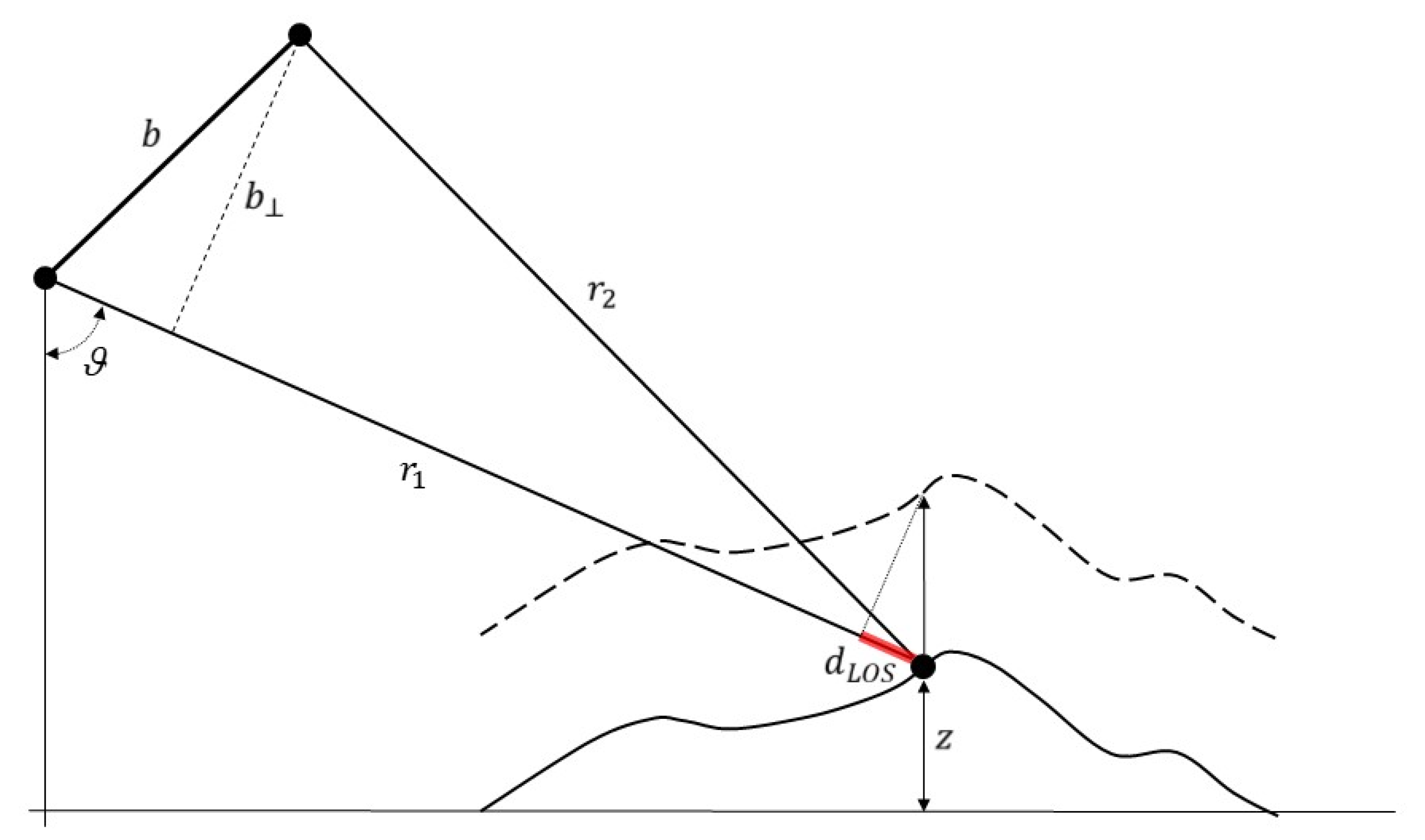
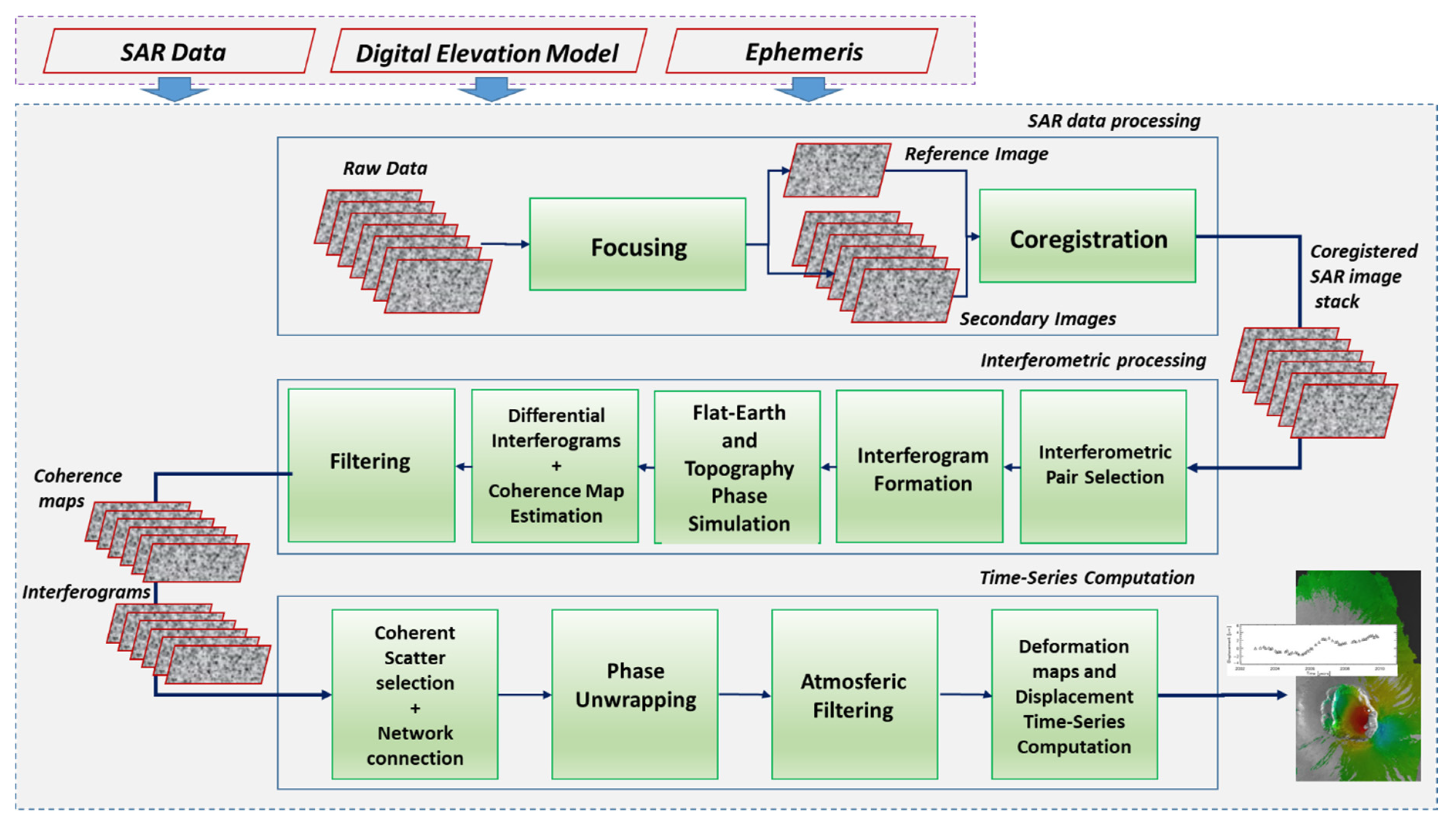
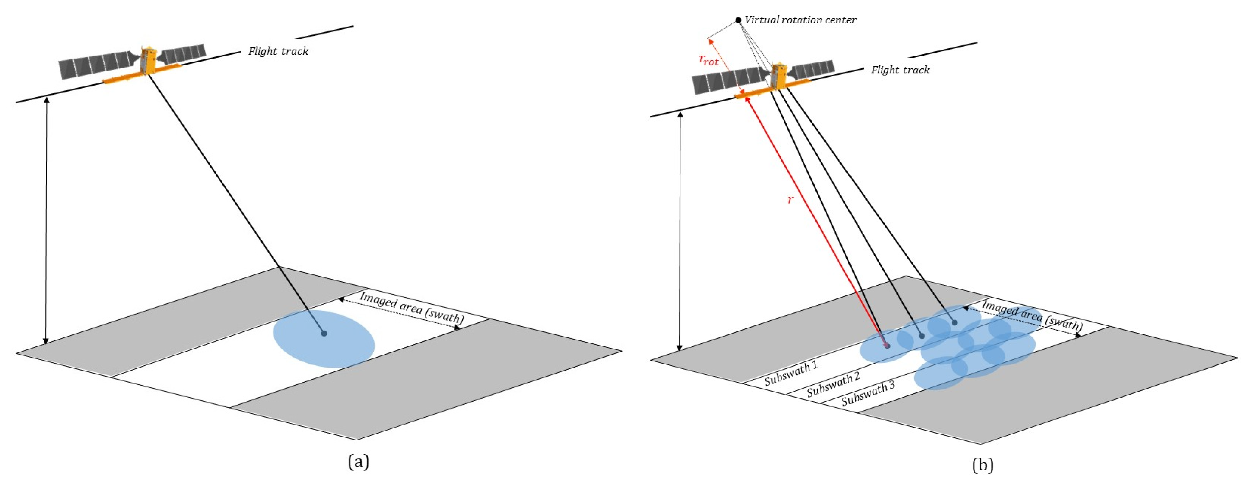
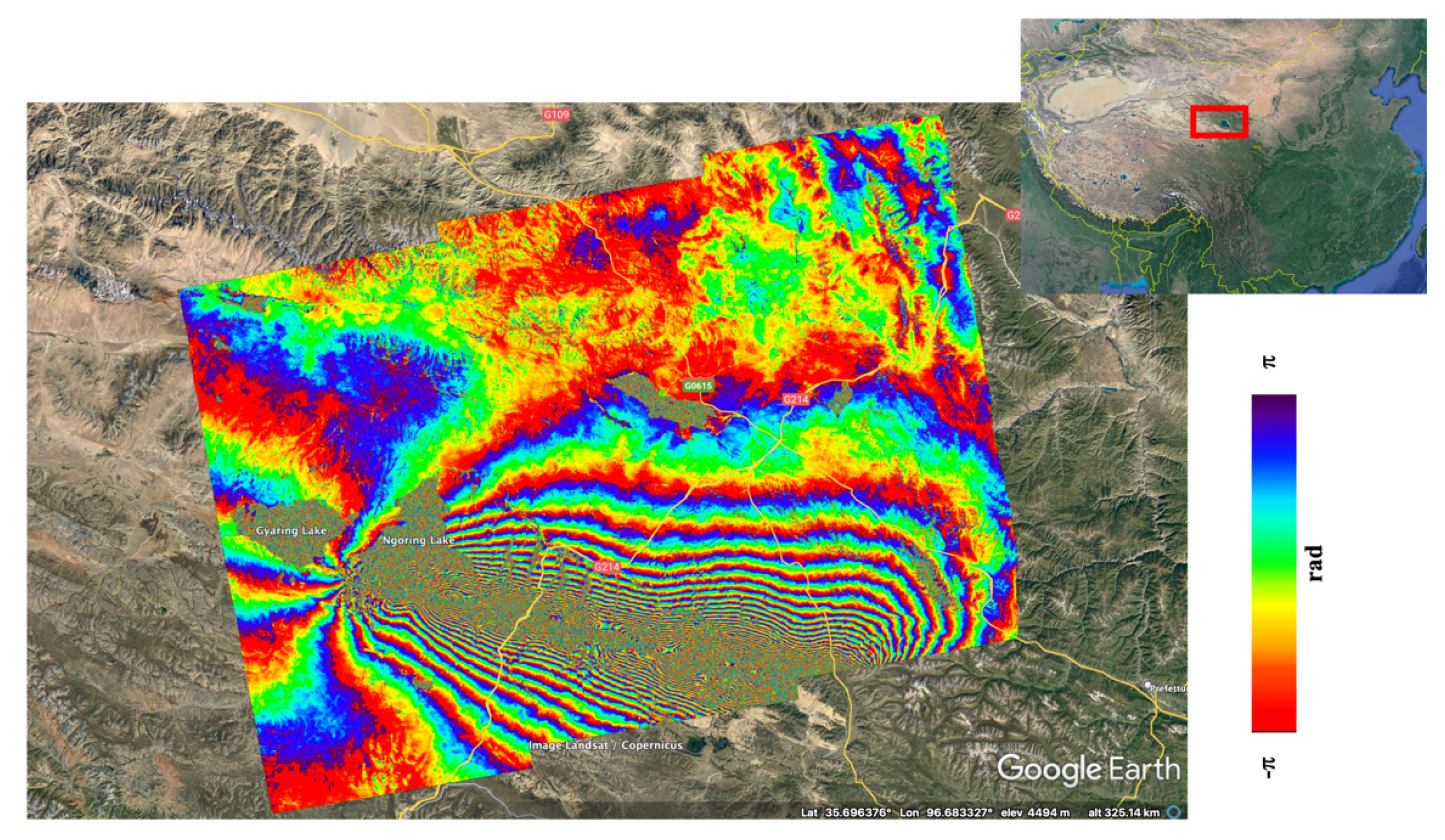
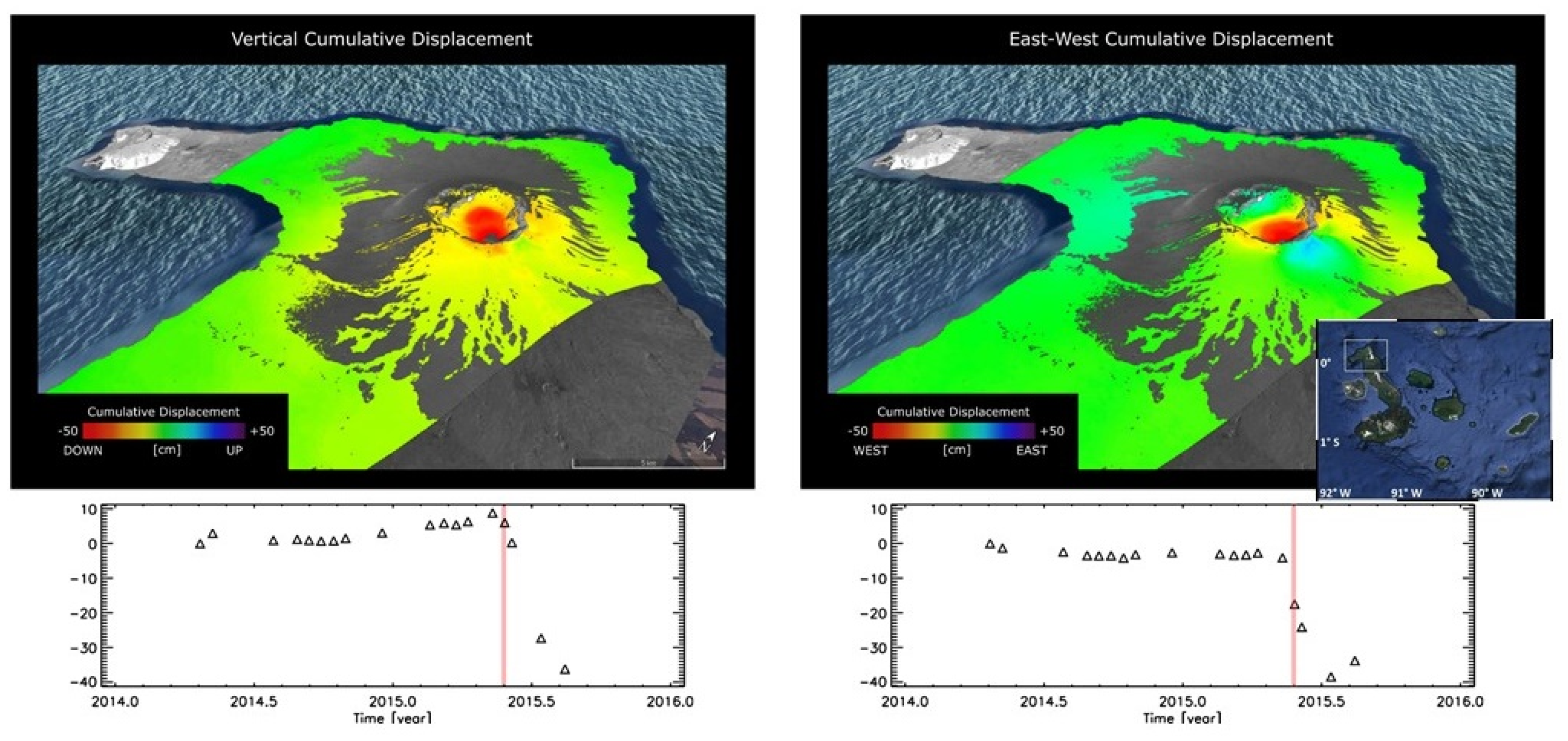
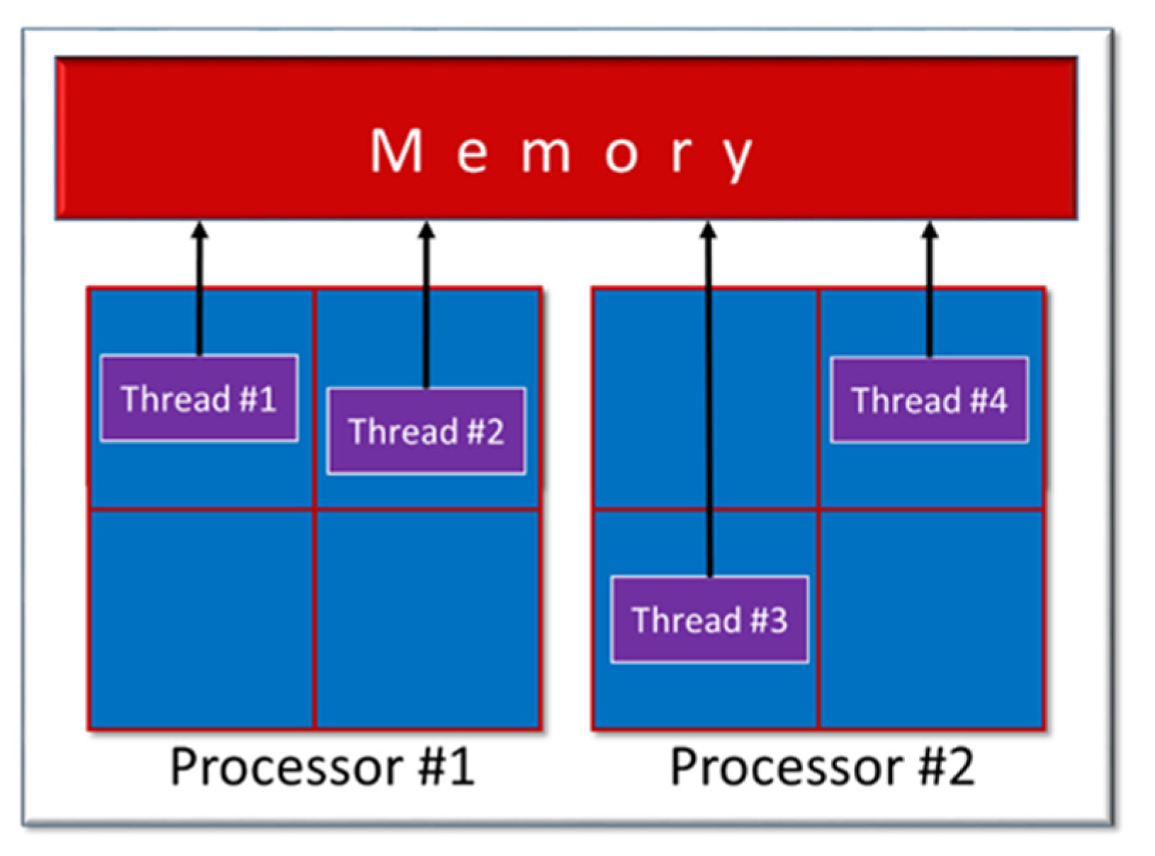
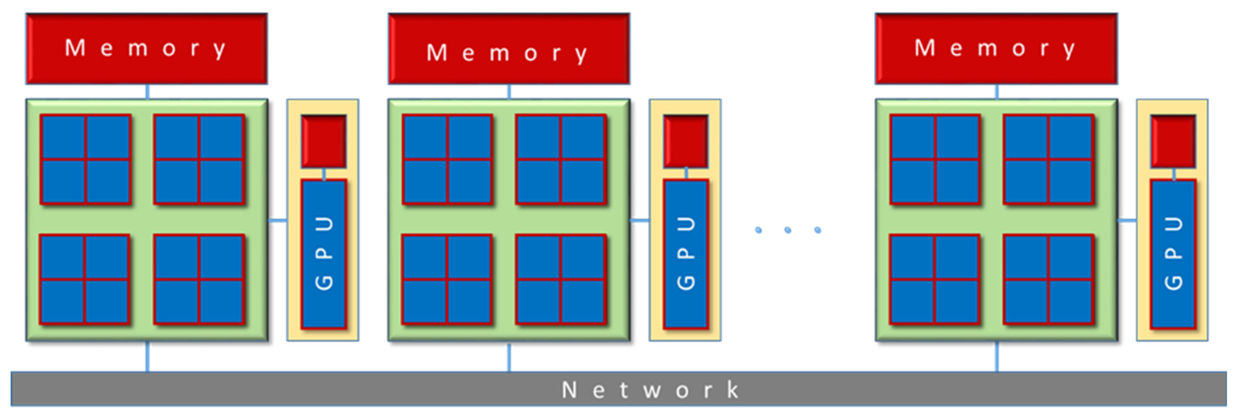
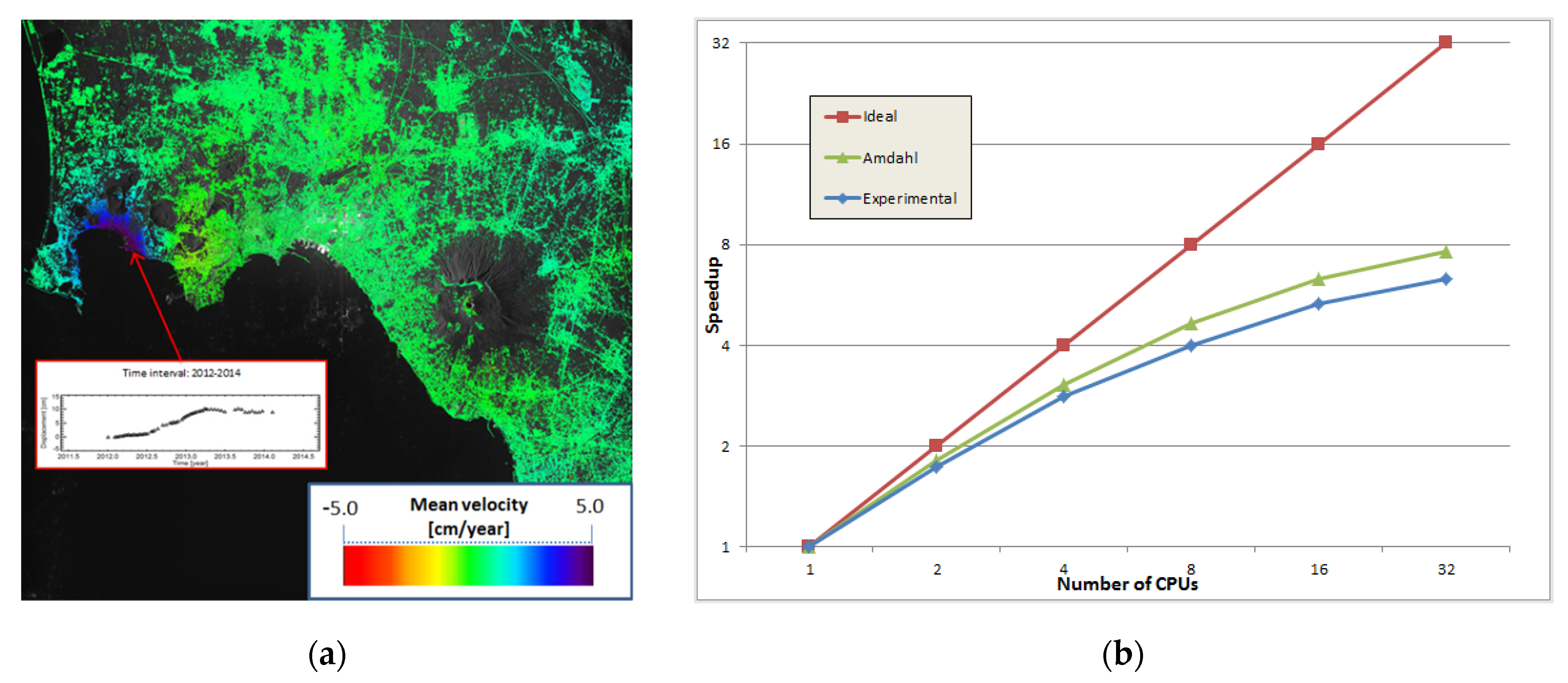
Table 1.
Operative and forthcoming SAR sensors.
| Sensor | Frequency | Agency/Country | Access | Revisit-Time | Resolution | Polarization | Frame Size | Year |
|---|---|---|---|---|---|---|---|---|
| TanDEM-L | L-band (1275 GHz, λ =24.6 cm) | German Aerospace Centre (DLR) | Free and open | 16 days | 7 m | Single, dual, quad mode | dual-pol mode 350 km quad-pol mode: 175 km | ≥2024 |
| BIOMASS | P band (435 MHz, λ = 70 cm) | European Space Agency (ESA) | Free and open | 17 days | 60 × 50 m | quad-pol | 50 × 50 km | ≥2023 |
| NISAR | S-band (3.2 GHz, λ = 9 cm) | NASA ISRO | Free and open | 12 days | 3–10 m | Single: HH,VV | >240 km | ≥2023 |
| Dual: HH/HV, VV/VH | ||||||||
| Compact: RH/RV | ||||||||
| Quasi-Quad: HH/HV, VH/VV | ||||||||
| L-band (1.26 GHz, λ = 24 cm) | Single: HH, VV Dual: HH/HV, VV/VH Compact: RH/RV Quad: HH/HV/VH/VV | |||||||
| RCM | C-band (5.4 GHz, λ = 5.6 cm) | Canadian Space Agency | Commercial | Satellite: 12 days Constellation: 4 days | 3–100 m | Single: HH, VV, VH, HV Dual: HH/HV, VV/VH, HH/VV Compact Quad | 20 × 20–500 × 500 km | 2019– |
| PAZ SAR | X band (9.65 GHz, λ = 3.5 cm) | Space Agency of Spain | Commercial | 11 days | Stripmap: 3–6 m ScanSAR: 16 × 6 m spotlight: 1–2 m | HH/VV/HV/VH (single or dual) | Stripmap: 30–2000 × 30 km ScanSAR: spotlight: 10 × 10 km | 2018– |
| TerraSAR-X Tandem-X | X band (9.65 GHz λ = 3.5 cm) | German Aerospace Centre (DLR) | Commercial; limited proposal-based scientific | 11 days | Spotlight: 0.2 × 1.0–1.7 × 3.5 m Stripmap: 3 × 3 m ScanSAR: 18–40 m | Single: HH, VV Dual: HH/VV, HH/HV, VV/VH Twin: HH/VV, HH/VH,VV/VH | Spotlight: 3–10 km Stripmap: 50 × 3 0 km ScanSAR: 150 × 100- 200 × 200 km | 2007–2010– |
| COSMO-SkyMed | X band (9.6 GHz λ = 3.5 cm) | Italian Space Agency (ASI) | Commercial; limited proposal-based scientific | Satellite: 16 days Constellation: 1–8 days | Spotlight: ≤1 m Stripmap: 3–15 m ScanSAR: 30–100 m | Single: HH, VV, HV, VH Dual: HH/HV, HH/VV, VV/VH | Spotlight: 10 × 10 km Stripmap: 40 × 40 km ScanSAR: 100 × 100–200 × 200 km | 2007– |
| Sentinel-1 | C band (5.4 GHz, λ = 5.6 cm) | European Space Agency (ESA) | Free and open | Satellite: 12 days Constellation: 6 days | Stripmap: 5 × 5 m Interferometric Wide Swath (IW): 5 × 2 0m Extra Wide Swath (EW): 20–40 m | Single: HH, VV Dual: HH/HV, VV/VH | Stripmap: 375 km IW: 250 km EW: 400 km | 2014– |
| RADARSAT-2 | C band (5.4 GHz, λ = 5.6 cm) | Canadian Space Agency | Commercial | 24 days | Spotlight: ~1.5 m Stripmap: ~3 × 3–25 × 25 m ScanSAR: 35 × 35–100 × 100 m | Single: HH, VV, HV, VH Dual: HH/HV, VV/VH Quad: HH/HV/VH/VV | Spotlight: 18 × 8 km Stripmap: 20–17 0 m ScanSAR: 300 × 300–500 × 500 km | 2007– |
| SAOCOM | L band (1275 GHz, λ = 24.6 cm) | Argentina National Space Activities Commission (CONAE) | Commercial; limited proposal-based scientific | Satellite: 16 days Constellation: 8 day | Stripmap: 10 × 10 m TopSAR: 100 × 100 m | Single: HH, VV Dual: HH/HV, VV/VH Quad: HH/HV/VH/VV | Stripmap: >65 km TopSAR: 320 km | 2018– |
| ALOS-2 PALSAR-2 | L band (1275 GHz, λ = 24.6 cm) | Japan Aerospace Exploration Agency (JAXA) | Commercial; limited proposal-based scientific | 14 days | Spotlight: 1 × 3 m Stripmap: 3–10 m ScanSAR: 25–100 m | Single: HH, VV, HV, VH Dual: HH/HV, VV/VH Quad: HH/HV/VH/VV | Spotlight: 25 × 25 km Stripmap: 55 × 70–70 × 70 km ScanSAR: 355 × 355 km | 2014– |
Table 2.
Summary of the reviewed InSAR Fundamental Stages using HPC.
| Processing Stage | Selected Works | Parallelism | Tools | Year |
|---|---|---|---|---|
| Focusing | [181,182] | Multithreading | OpenMP | 2016 |
| [183,184] | GPU-based | OpenCL | 2019 | |
| [185] | GPU-based | CUDA | 2020 | |
| [188] | GPU-based | CUDA | 2014 | |
| [186] | GPUs + CPUs | CUDA/OpenMP | 2016 | |
| [189] | multi-GPU | CUDA/MPI | 2018 | |
| [187] | GPU-based | CUDA | 2016 | |
| Coregistration | [190] | Multiprocessing | MPI | 2002 |
| [49] | Multithreading | OpenMP | 2021 | |
| [191] | GPU-based | CUDA | 2014 | |
| [192] | GPU-based | CUDA | 2020 | |
| Phase Unwrapping | [198] | Dual-level | MPI/OpenMP | 2015 |
| [196,197] | Dual-level | MP/OpenMP | 2015 | |
| [199] | Multithreading | OpenMP | 2015 | |
| [200] | GPU-based | CUDA | 2014 | |
| [201] | GPU-based | CUDA | 2017 | |
| InSAR Filtering | [190] | Multiprocessing | MPI | 2015 |
| [194] | GPU-based | CUDA | 2016 | |
| [195] | GPU-based | OpenCL | 2020 |
Publisher’s Note: MDPI stays neutral with regard to jurisdictional claims in published maps and institutional affiliations. |
© 2021 by the authors. Licensee MDPI, Basel, Switzerland. This article is an open access article distributed under the terms and conditions of the Creative Commons Attribution (CC BY) license (https://creativecommons.org/licenses/by/4.0/).
Share and Cite
MDPI and ACS Style
Imperatore, P.; Pepe, A.; Sansosti, E. High Performance Computing in Satellite SAR Interferometry: A Critical Perspective. Remote Sens. 2021, 13, 4756. https://0-doi-org.brum.beds.ac.uk/10.3390/rs13234756
AMA Style
Imperatore P, Pepe A, Sansosti E. High Performance Computing in Satellite SAR Interferometry: A Critical Perspective. Remote Sensing. 2021; 13(23):4756. https://0-doi-org.brum.beds.ac.uk/10.3390/rs13234756
Chicago/Turabian StyleImperatore, Pasquale, Antonio Pepe, and Eugenio Sansosti. 2021. "High Performance Computing in Satellite SAR Interferometry: A Critical Perspective" Remote Sensing 13, no. 23: 4756. https://0-doi-org.brum.beds.ac.uk/10.3390/rs13234756
Note that from the first issue of 2016, this journal uses article numbers instead of page numbers. See further details here.