A Case Study of the 3D Water Vapor Tomography Model Based on a Fast Voxel Traversal Algorithm for Ray Tracing

Abstract

A fast voxel traversal algorithm for ray tracing was applied to build a 4 × 4 × 20 tomography model using the observation data of 11 ground-based Global Navigation Satellite System (GNSS) meteorology (GNSS/MET) stations in Hebei Province, China. The precipitation water vapor (PWV) observed at 05 a.m. (Universal Time Coordinated: UTC) on 10 December 2019, was used to reconstruct three-dimensional (3D) water vapor density fields over the test area. The tomographic results (GNSS_T) show that the water vapor density above this area is mainly below 25 g/m³ and is concentrated between the first to the fourth layers. The vertical distribution conforms to the exponential characteristics, while the horizontal distribution shows a decreasing trend from southwest to northeast. In addition, the results of the 0.25° grid dataset generated by the Global Forecast System (GFS) of the National Center for Environmental Forecasting (NCEP) (GFS_L) were interpolated to the height of the tomographic grid, which is in good agreement with the tomographic results. GFS_L is larger than GNSS_T on the first floor at the surface, with an average deviation of 0.19 g/m³. In contrast, GFS_L from the second floor to the top of the model is smaller than GNSS_T, with the average deviations distributed between −0.08 and −0.15 g/m³.

1. Introduction

Changes in water vapor over time and space have particularly important indications for meteorological forecasting [1,2], especially for the monitoring and forecasting of small-and medium-scale severe weather with a horizontal scale of about 100 km and a life history of only a few hours [3,4,5]. Its 3D distribution is critical for the development and correction of the initial field of the mesoscale numerical forecasting model. Accurate atmospheric water vapor monitoring and its assimilation in the numerical weather forecasting model will improve the prediction accuracy of precipitation and severe weather [6,7]. The initial value of the 3D spatial distribution of water vapor in the current model is mainly provided by the radiosonde network, which takes observations every 12 h, and the distance between the stations is higher than 200 to 300 km [5]. Although aircraft observations, satellite, and ground data have been used as supplementary observations to initialize mesoscale models in recent years, their applications are limited by the lower spatial resolution and retrieval accuracy [8,9].

Meteorological products such as precipitable water vapor (PWV), total zenith delay (ZTD), and zenith wet delay (ZWD) obtained by ground-based Global Navigation Satellite System (GNSS) meteorology can accurately describe the details of high temporal and spatial changes of atmospheric water vapor in real-time. Moreover, satellite navigation systems such as Global Positioning System (GPS), BeiDou Navigation Satellite System (BDS), and Global Navigation Satellite System (GLONASS) are developing rapidly, and their observation ranges can cover the whole world [10,11,12], which solves the difficulties in weather forecasts [5,13]. The assimilation of PWV data has a positive impact on temperature, humidity, and precipitation forecasting [14,15,16,17,18,19], but the application of PWV also has a bottleneck because it cannot reflect the 3D distribution of water vapor in the atmosphere. To address this limitation, the slant water vapor (SWV) measured by GNSS contains the vertical profile information of water vapor. By using the observation data of the slant path of the GNSS network with densely distributed stations, the 3D distribution of water vapor can be obtained by a tomography technique [20,21,22,23]. By comparing the vertical distribution of water vapor retrieved from 3D tomography with the results obtained by numerical weather models [24], accurate vertical structure of deviations can be obtained to capture the continuously changing processes of small-scale water vapor fields during strong convection [21]. This will play a positive role in improving the GNSS observation data assimilation operator and the humidity field of the numerical prediction during convection [25]. Flores et al. [26] used the slant wet delay (SWD) to detail the tomography of atmospheric water vapor through the discretion of the tropospheric atmosphere over the GNSS area, and by using SWD across the grid in all directions to obtain the water vapor information in the grid. Moreover, Hirahara [27] conducted a tomographic experiment in Shigaraki to study the changes in atmospheric water vapor over a large scale and obtained a four-dimensional wet refractive index structure during a cold front transit. Meanwhile, MacDonald et al. [28] compared the SWD with other observations and pointed out that the denser the GPS monitoring network is, the easier it is to detect the 3D distribution of water vapor. Braun et al. [1] and Braun and Rocken [29] established the relationship between the SWD and the amount of SWV and verified the accuracy and feasibility of GPS remote sensing of water vapor in a slant path. Sparse rays passing through the model grid can cause ill-condition issues during tomography. Benevides et al. [30] used multi-GNSS observations to tackle this problem, while Yao and Zhao [31] added the rays passing through the side of the tomographic model into the observation equation matrix to increase the stability of the calculation. In recent years, many researches have focused on the model building technology itself, some new methods and techniques such as the least-squares and compressive sensing [32], improved parameterized tropospheric tomographic technique [33], and adaptive simultaneous iterative reconstruction technique [34] have been applied to the model. In addition, many studies resolved the problems of solving observing equations [35,36] while some other studies took the observations of multi-satellite navigation systems as input [37,38] to promote the efficiency of the model. However, few studies have focused on the efficiency of signal line indexing in the tomography model which also needs to be improved.

Tracing rays through the grid index during the tomography process consumes computing resources and is prone to aliasing. The traditional index determination method requires the coordinates of the intersection point of the ray and the grid and then finds the midpoint coordinates of two adjacent intersection points [39]. This process consumes more than 75% of the computing resources [40]. The DDA (digital differential analyzer) algorithm is the simplest straight-line algorithm in computer graphics and can be used for ray tracing. The basic idea is a numerical differential algorithm [41,42], yet Fujimoto et al. [43] extended the two-dimensional DDA algorithm to three dimensions. The three-dimensional DDA (3DDDA) algorithm improves the ray tracing calculation speed by 13 times compared to the traditional algorithms. Amanatides and Woo [44] introduced a fast voxel traversal algorithm for ray tracing, which is an improvement of the DDA algorithm as it does not require unconditional stepping along an axis like 3DDDA and it has no preferred axis. It greatly simplifies the internal loop and realizes an accurate judgment of whether the intersection of the ray and grid is in the current index.

In this study, the fast voxel traversal algorithm for ray tracing was applied to the 3D water vapor tomography model for the first time, which not only eliminated the complicated process of calculating the center point of the signal line in the grid during the indexing process but also solved the problem of repeated indexing when the signal line crosses the grid intersection line. Consequently, it improved the indexing efficiency of the signal line and provided accurate grid intercept positioning information for observation equations. We conducted a tomography test using the slant water vapor (SWV) observed by 11 stations in Hebei, China, then used the GFS reanalysis data at the same site to compare with the GNSS tomography results to quantitatively evaluate the solution of the tomographic model which provides a reference for tomography application of the fast voxel traversal algorithm.

2. Materials and Methods

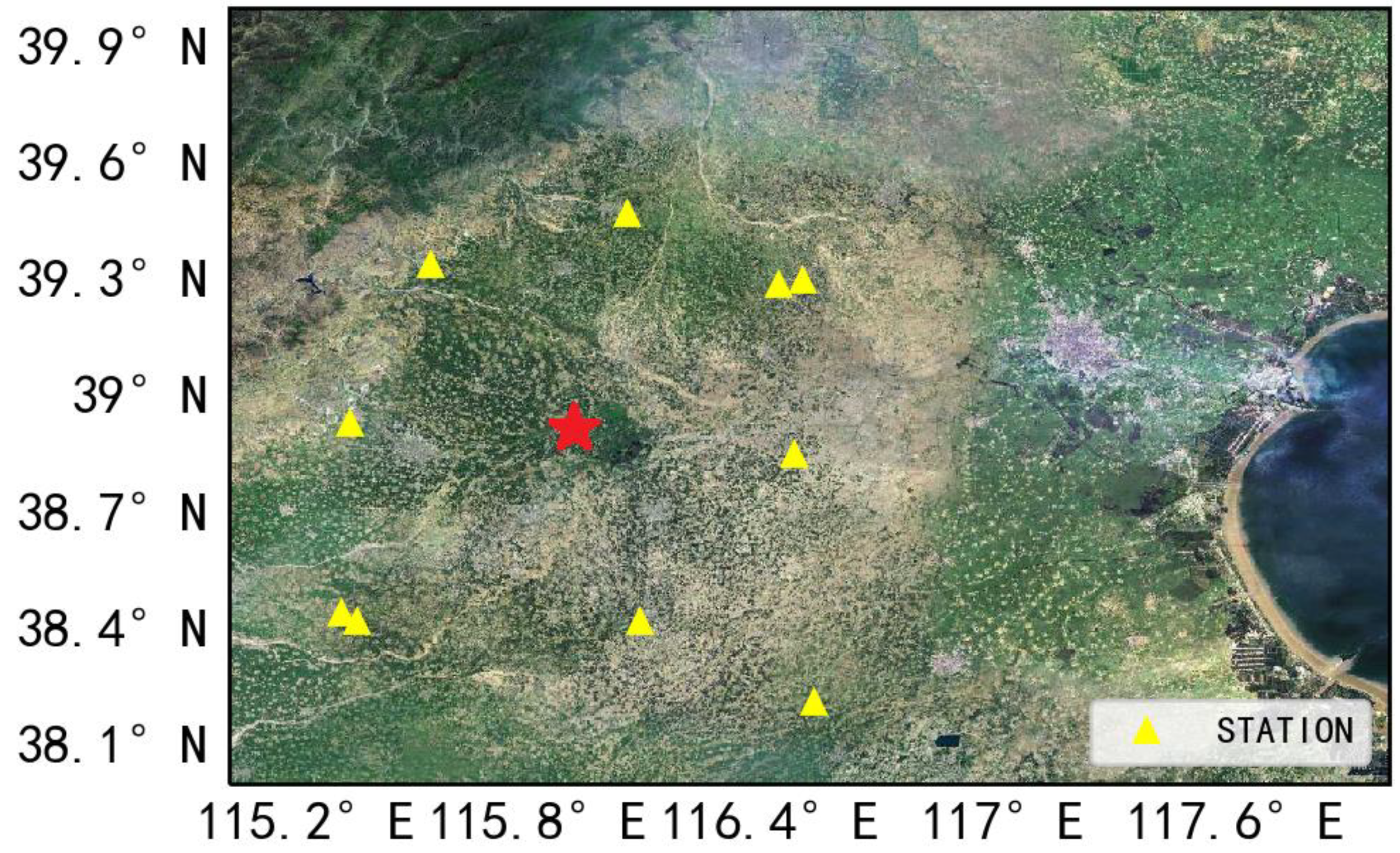
2.1. Data Introduction

This tomography experiment used the observation data of 11 GNSS/MET stations in Hebei Province, China, at 05 a.m. (UTC) on 10 December 2019. The parameters, such as the position of the stations and equipment models, are shown in

Table 1. The parameters of the station.

Station	Latitude	Longitude	Altitude (km)	Receiver	Antenna
szcz	38.21°N	116.51°E	0.008	TRIMBLE NETR9	TRM57971.00
szag	38.42°N	115.33°E	0.036	TRIMBLE NETR9	TRM55971.00
szhj	38.42°N	116.06°E	0.015	TRIMBLE NETR9	TRM57971.00
szbd	38.44°N	115.29°E	0.017	TRIMBLE NETR9	TRM57971.00
szwe	38.85°N	116.46°E	0.008	TRIMBLE NETR9	TRM57971.00
szme	38.93°N	115.31°E	0.05	TRIMBLE NETR9	TRM57971.00
szax	38.94°N	115.89°E	0.013	TRIMBLE NETR9	TRM57971.00
szlf	39.29°N	116.42°E	0.014	TRIMBLE NETR9	TRM57971.00
szyq	39.3 °N	116.48°E	0.016	TRIMBLE NETR9	TRM57971.00
szyx	39.34°N	115.52°E	0.056	TRIMBLE NETR9	TRM55971.00
szzz	39.47°N	116.03°E	0.036	TRIMBLE NETR9	TRM57971.00

.

The Global Forecast System (GFS) dataset used for the verification and analysis of water vapor tomography results in this study is the reanalysis result of the NCEP grib2 format global forecast system running on a 0.25° × 0.25° global grid. The air pressure stratification is divided into 50 layers between 0.4 hPa and 1000 hPa, and the product interval is 3 h. The meteorological elements used were temperature, relative humidity, potential height, and air pressure of each layer. The address to download the data is as follows: https://rda.ucar.edu/datasets/ds084.1/, accessed on 12 January 2020.

2.2. Methodology

The total delay distance of the GNSS signals in the atmosphere $\mathsf{\Delta }L$ is related to the atmospheric refractivity N [45],

$$\mathsf{\Delta }L={{\displaystyle \int }}_{s}Nds$$

(1)

N can be expressed in terms of atmospheric properties as follows [46],

$$N=\left[-4.03\times {10}^6\frac{n_e}{f}\right]+\left[77.6\frac{P_d}{T}\right]+\left[70.4\frac{P_v}{T}+3.739\frac{P_v}{T^2}\right]$$

(2)

where $n_e$ is the electron density in the atmosphere, f is the frequency of the electromagnetic wave, $P_d$ is the pressure of the dry air, $P_v$ is the pressure of the humid air, and T is the atmospheric temperature. The above formula can be understood as the $ZTD$, calculated as the sum of the zenith hydrostatic delay ($ZHD$) and $ZWD$. $ZHD$ can be calculated accurately based on Saastamoinenempirical formulas [47]. Then $ZWD$ can be obtained by subtracting $ZHD$ from the $ZTD$.

$ZWD$ has a relationship with $PWV$ which is proved by Bevis et al. [45],

$$PWV=\prod \times ZWD$$

(3)

${\displaystyle \prod }$ is the mapping function calculated as follows [45],

$$\prod =\frac{{10}^6}{\rho R_v[\frac{k_3}{T_m}+k_2-\omega k_1]}$$

(4)

where $\rho$ is the water vapor density, $R_v$ is an atmospheric constant of water vapor, $k_1$, $k_2$, $k_3$, and ω are physical constants, and $T_m$ is the average temperature of the atmosphere, which can be expressed by the surface air temperature: $T_m=70.2+0.72T_s$. The radiosonde data can be used for regression analysis to establish coefficient values suitable for the characteristics of the area [45].

PWV cannot be directly used for 3D tomography calculation, and the total amount of atmospheric water vapor in the zenith direction needs to be converted into the water vapor content on the satellite’s slant path using a mapping function. The total tropospheric delay ($STD$) can be expressed as [48],

$$STD=M_{dry}\left(e\right)ZHD+M_{wet}\left(e\right)ZWD+M_{\mathsf{\Delta }}\left(e\right)\left(G_N\cos (\varnothing )+G_E\sin (\varnothing )\right)$$

(5)

where $M_{dry}\left(e\right)$ and $M_{wet}\left(e\right)$ represent the dry and wet mapping functions, respectively; $G_N$ and $G_E$ represent the north-south and east-west gradients, respectively; $M_{\mathsf{\Delta }}\left(e\right)$ is the horizontal gradient mapping function; e is the satellite elevation angle, and; $\varnothing$ is the satellite azimuth angle. When using the GAMIT software [49] for data processing, $ZTD$ and the total delay gradient are first to be calculated. Then, the method described above is used to obtain $ZWD$. Equation (3) shows that $PWV$ and $ZWD$ can be directly converted according to the coefficient, so formula (5) can be converted into the form that directly uses $PWV$. $SW{V}_i^k$ represents the slant path moisture content of the satellite $k$ received by station $i$, $\lambda$ = 0.15 [48], and $PW{V}_i$ is the total amount of precipitable water vapor over station $i$ [48].

$$SW{V}_i^k=M_{wet}(e_i^k)PW{V}_i+\lambda \times [M_{\mathsf{\Delta }}\left(e\right)\left(G_N^w\cos (\varnothing )+G_E^w\sin (\varnothing )\right)$$

(6)

GAMIT does not generate dry and wet delay gradients separately. The dry delay gradient is stable, which can be assumed as a constant for a certain period of time (12 h). By averaging the gradient solutions $G_N$ and $G_E$ in this period, the influence of the dry delay gradient can be reduced or eliminated, then the wet delay gradients $G_N^w$ and $G_E^w$ can be obtained. The wet mapping function can be calculated using the following formula [50],

$$M_{wet}\left(e_i^k\right)=\frac{1+a_w/\left(1+b_w/\left(1+c_w\right)\right)}{\sin e+a_w/\left(\sin e+b_w/\left(\sin e+c_w\right)\right)}$$

(7)

$M_{wet}\left(e_i^k\right)$ represents the wet mapping function of station $i$, receiving satellite $k$, while $a_w$, $b_w$, and $c_w$ are the parameters of the new mapping function developed by [51] related to the geographic location and date but have no connection with the meteorological observations, which can be calculated using formula (8).

$$a_w=a_{avg}\left({\phi }_i\right)-a_{amp}\left({\phi }_i\right)\cos (2\gamma \times \frac{t-T_0}{365.25})$$

(8)

where $\gamma$ = 3.14, $a_{avg}\left({\phi }_i\right)$ and $a_{amp}\left({\phi }_i\right)$ can be queried in [51], ${\phi }_i$ represents the latitude of station $i$, t is the day of year, $T_0$ = 28; and $b_w$ and $c_w$ are obtained by the same method. The mapping function of the horizontal gradient is calculated according to the following formula, where c = 0.0032 [48].

$$m_{\mathsf{\Delta }}\left(e\right)=1/\left(\sin \left(e\right)\tan \left(e\right)+c\right)$$

(9)

3. Model Building

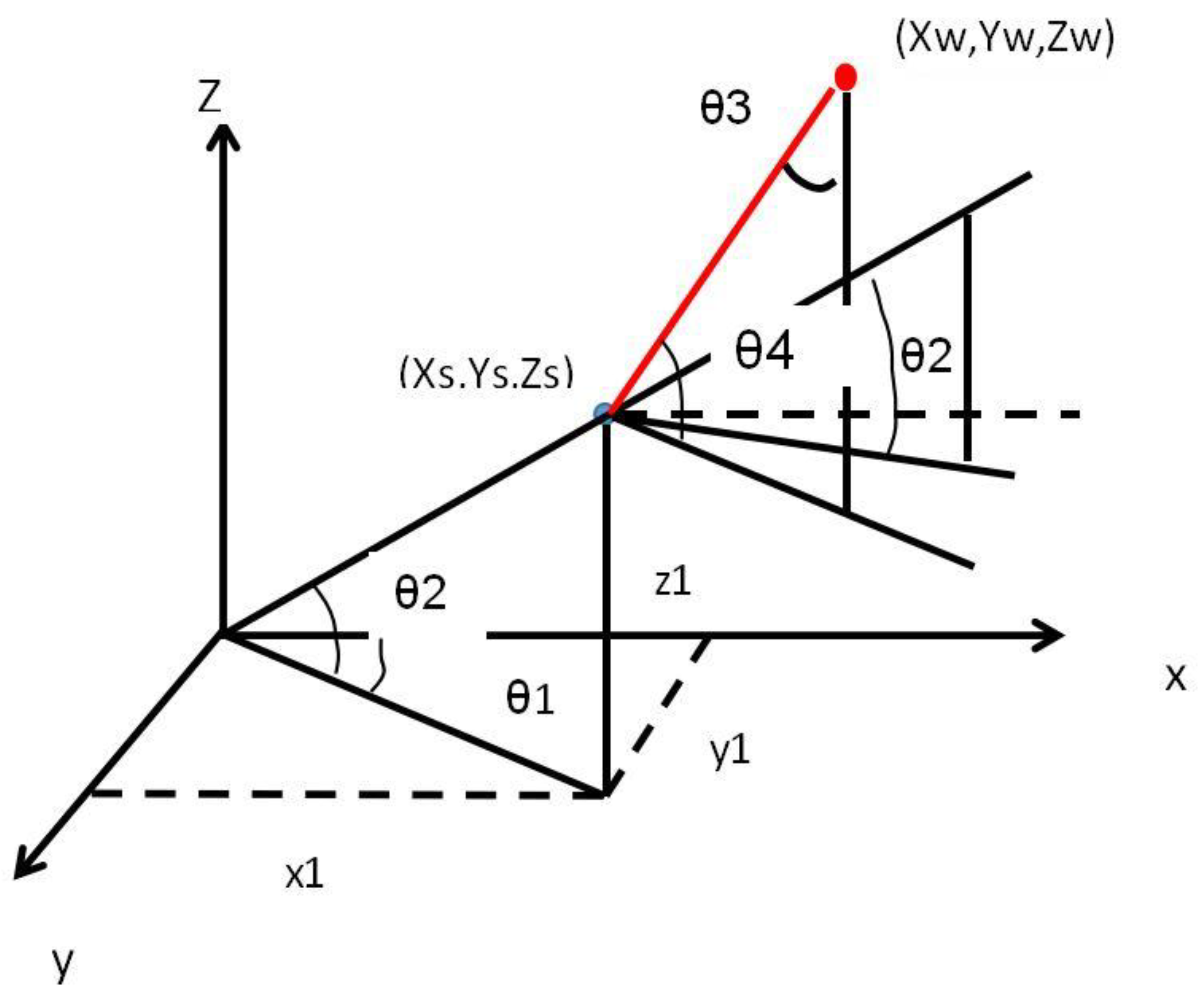
3.1. Unification of Coordinate System

First, the ground-based GNSS observation data from 11 stations in Hebei Province were selected as the input of the tomography model, as shown in Figure 1. The coordinates of the station in the middle position were selected as the origin (red star) of the new coordinate system, and the relative coordinates of other stations were calculated.

Second, generate a 4 × 4 × 20 basic grid with the station in the middle position as the origin. In the horizontal direction, the area of $2^{°}\times 2^{°}$ is divided into 4 × 4 uniform grids, and in the vertical direction, the 10 km is divided into 20 layers evenly. Then, the coordinates of the intersection point between the signal line and the top layer of the model were calculated based on the relative coordinates of each station and the satellite elevation and azimuth angles. Assuming that the elevation angle of the satellite is θ, the azimuth angle is $\alpha$, the wgs84 coordinates of the station are $lo{n}_s$, $la{t}_s$, $h_s$, and the intersection point of the satellite ray and the ceiling of the model are $lo{n}_d$, $la{t}_d$, $h_d$.

If 0°< $\alpha$ ≤ 90°,

$$lo{n}_d=\frac{\left(10-\left(h_s/1000\right)\right)}{\tan \theta }\times \sin \alpha +lo{n}_s$$

(10)

$$la{t}_d=\frac{\left(10-\left(h_s/1000\right)\right)}{\tan \theta }\times \cos \alpha +la{t}_s$$

(11)

If 90°< $\alpha$ ≤ 180°,

$$lo{n}_d=\frac{\left(10-\left(h_s/1000\right)\right)}{\tan \theta }\times \sin \left({180}^{°}-\alpha \right)+lo{n}_s$$

(12)

$$la{t}_d=\frac{\left(10-\left(h_s/1000\right)\right)}{\tan \theta }\times \cos \left({180}^{°}-\alpha \right)+la{t}_s$$

(13)

If 180° < $\alpha$ ≤ 270°,

$$lo{n}_d=\frac{\left(10-\left(h_s/1000\right)\right)}{\tan \theta }\times \sin \left(\alpha -{180}^{°}\right)+lo{n}_s$$

(14)

$$la{t}_d=\frac{\left(10-\left(h_s/1000\right)\right)}{\tan \theta }\times \cos \left(\alpha -{180}^{°}\right)+la{t}_s$$

(15)

If 270°< $\alpha$ ≤ 360°,

$$lo{n}_d=\frac{\left(10-\left(h_s/1000\right)\right)}{\tan \theta }\times \sin \left({360}^{°}-\alpha \right)+lo{n}_s$$

(16)

$$la{t}_d=\frac{\left(10-\left(h_s/1000\right)\right)}{\tan \theta }\times \cos \left({360}^{°}-\alpha \right)+la{t}_s$$

(17)

$h_d$ = 10,

If $\alpha$ ≤ 0°, $\alpha$ =$\alpha$ + 360°, then repeat the judgment above.

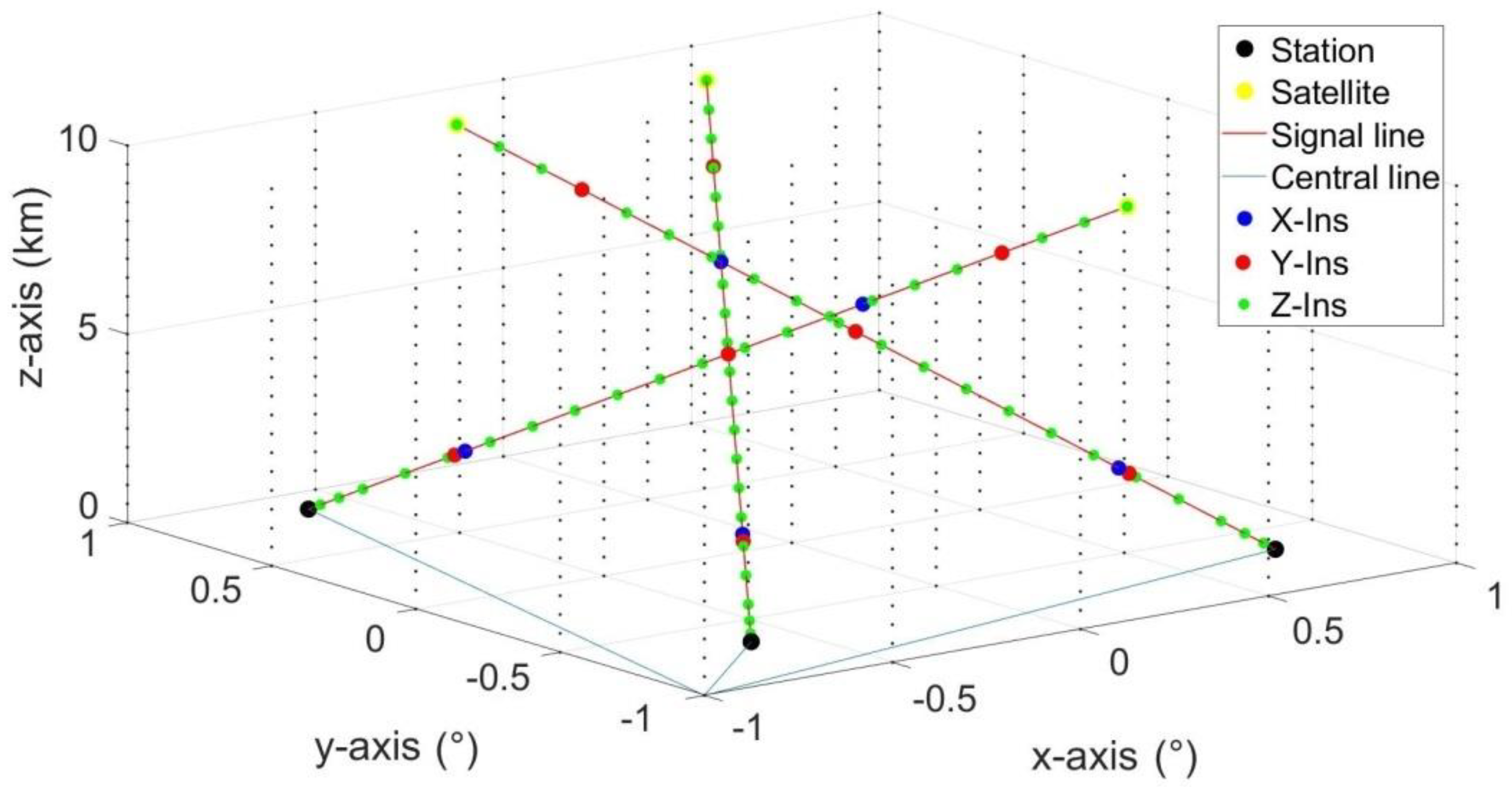
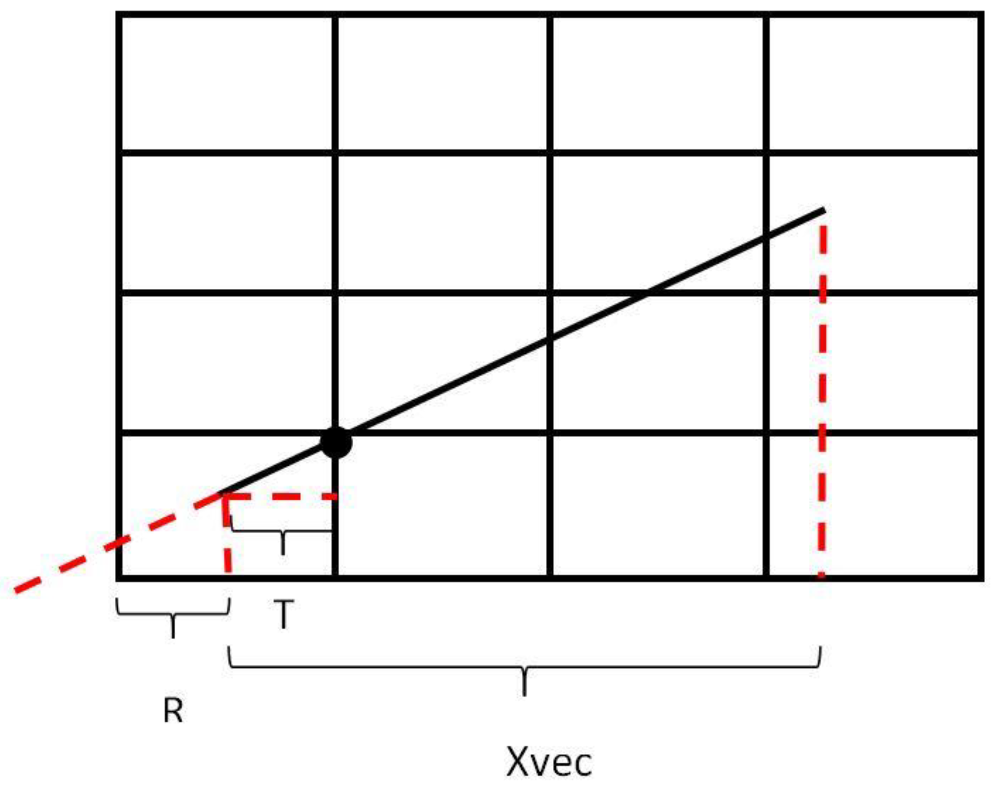
3.2. The Intercept of the Signal Line and the Grid

The surface perpendicular to the X-axis is defined as the X-axis profile, and the Y-axis and Z-axis profiles are named in the same way. Taking the intersection of the signal line and the Z-axis profile as an example, the red line represents the signal line in Figure 2, the red line represents the satellite position, and the blue origin represents the station position. ${\theta }_1=\arctan \left(Y_1/X_1\right)$, ${\theta }_2=\arctan \left(Z_1/\mathrm{sqrt}\left(X_1^2+Y_1^2\right)\right)$ [52],

$$\begin{array}{c}{\theta }_3=\arctan (\left(Z_w-Z_s\right)/\mathrm{sqrt}(\left(X_w-X_s\right)^2+\left(Y_w-Y_s\right)^2\\ +\left(Z_w-Z_s\right)^2))\end{array}$$

(18)

${\theta }_4={90}^{°}-{\theta }_3$, By using the sine of ${\theta }_4$ to project the distance between the grids in the X-axis direction into the distance between the intersections on the signal line, the intersection coordinate of the X-axis profile and the signal line can be obtained by using the range limit of the X value. According to the same method, the intersection coordinates of the signal line and the Y (Z) axis profile can be calculated, as shown in Figure 3. Therefore, by sorting all the intersection coordinates obtained above according to the Z coordinate, the spatial position order of all intersections can be obtained. Because the coordinates of all the stations and satellites are positive, and the signal line is always along the Z-axis from small to large values, the distance between the intersection points is calculated to obtain the intercept of the signal line through each grid [53].

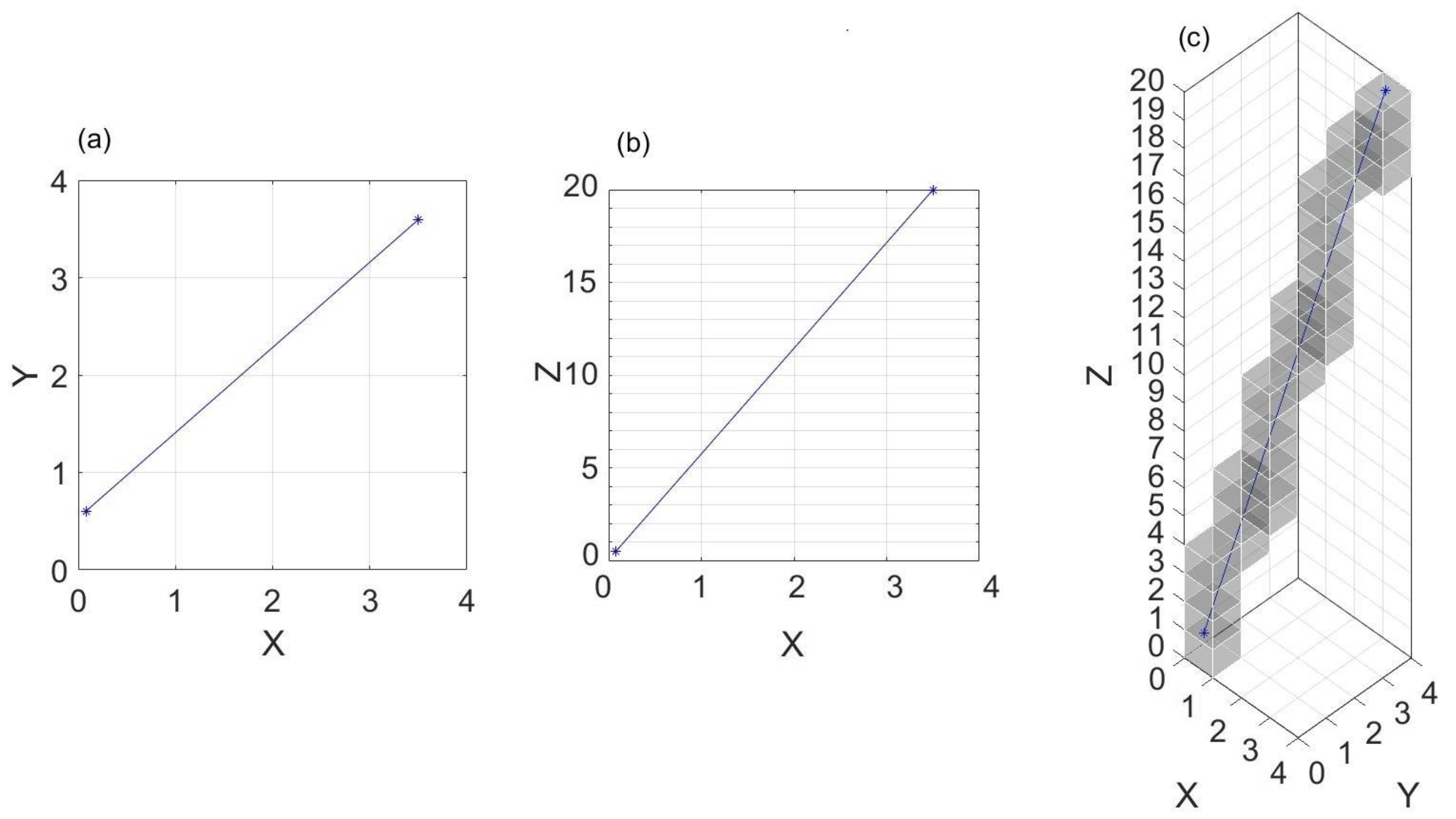
3.3. Indexing by a Fast Voxel Traversal Algorithm for Ray Tracing

Finding the index of the ray passing through the model grid is a key step in water vapor tomography modeling. Figure 4 shows the fast voxel traversal algorithm for ray tracing in a 2D grid. There are two important steps in the fast voxel traversal algorithm for ray tracing. First, the index of the starting point of the ray is determined using $X_{start}$ to represent the starting point of the X-axis of the signal line, while GridX[0] represents the starting point of the X-axis of the grid, and then whether $R=X_{start}-GridX\left[0\right]$ is greater than 0 can be determined. If it is greater than 0, the signal line is in the grid model, meaning that the next step is to calculate the starting index of the signal line. $X_{Index}^{start}$ Assuming that voxel size X represents the unit length of the X-axis of the grid,

$$X_{Index}^{start}=Max\left(1,ceil\left(\left(X_{start}-Grid\left[0\right]\right)/voxelsizeX\right)\right)$$

(19)

After the starting point index is determined, the direction of the signal line should be determined, and the scale of the X-axis direction is defined as

$$t_{max}X=\left(X_{Index}^{start}·voxelsizeX-X_{start}\right)/X_{vec}$$

(20)

where $X_{vec}$ represents the total projection length of the signal line on the X-axis. In the same way, the scales in the Y- and Z-axis directions can be obtained by $t_{max}Y$ and $t_{max}Z$, respectively, and then the three scales can be compared. The index number is one step forward in the direction of the minimum value, and the pointer is used to move the scale, which can effectively improve the tracking efficiency of the signal line. Therefore, it can be determined that the index number of the end of the signal line is similar to the start index, and it ends when the signal line advances to the index number $X_{Index}^{end}$,

$$X_{Index}^{end}=Max\left(1,ceil\left(\left(X_{end}-GridX\left[0\right]\right)/voxelsizeX\right)\right)$$

(21)

The index tracking of the signal line in the experiment is shown in Figure 5. The two figures on the left are the projections of the signal line on the XY and XZ profiles, and the right figure shows the index tracking result of the signal line in the 3D grid [54].

3.4. Formation and Solution of Equation Group

This section may be divided into subheadings. It should provide a concise and precise description of the experimental results, their interpretation, as well as the experimental conclusions that can be drawn.

3.4.1. Observation Equation

The signal line passes through each grid and generates an intercept, which is the coefficient of the observation equation. The water vapor density in the grid is the parameter to be determined, and the slant water vapor in the direction of the signal is the observed value. First, the intercept $S_i$ between the intersection points must be calculated, and then the intercept $S_i$ and index $N_i$ are stored correspondingly.

$$S_i=\sqrt{\left(x_{i+1}-x_i\right)^2+\left(y_{i+1}-y_i\right)^2+\left(z_{i+1}-z_i\right)^2}$$

(22)

The slant water vapor that each station receives from each signal is extracted, where s represents the number of satellites and n represents the number of stations. In this experiment, s = 9 and n = 11. Then, the observation equation of this experiment can be expressed as follows,

$$\left[\begin{array}{c}\begin{array}{c}{S}_{11}{S}_{12}\dots S_{1m}\\ S_{21}{S}_{22}\dots S_{2m}\\ \dots \dots \dots \end{array}\\ S_{t1}{S}_{t2}\dots S_{tm}\end{array}\right]·\left[\begin{array}{c}{X}_1\\ X_2\\ \dots \\ X_m\end{array}\right]=\left[\begin{array}{c}\begin{array}{c}SW{V}_1^1\\ SW{V}_1^2\end{array}\\ \dots \\ SW{V}_n^s\end{array}\right]$$

(23)

The first row of the matrix on the left represents all intersections with the grid when the signal line of the first satellite received by the first station passes through the grid. The intercept between the two intersections is the intercept, and the index corresponding to the intercept is the number of grids. For example, if the signal passes through the first grid, then the corresponding intercept is written to the position of $S_{11}$, and if it passes through the last grid m, then the corresponding intercept is written to the position of $S_{1m}$, m represents the total number of model grids, $t=s\times n$, and $X_i$ is the density of water vapor in each grid, which needs to be solved in this experiment.

3.4.2. Horizontal Constraint Matrix Equation

The geometric construction of the ground-based GNSS observation network and the uneven distribution of GPS satellites in the observation network made it difficult to provide observations that uniformly cover all grids. As a result, some grids have no observations passing through, thus the observation equation will be ill-conditioned. Assuming that the horizontal distribution of water vapor during the observation period is stable, the horizontal constraint is added to the observation equation based on the principle that the closer the distance is, the stronger the correlation. Grids with observational information can pass water vapor information to empty grids through horizontal constraints and fully transmit the information of observations to all grids. Generally, the horizontal constraint uses a Gaussian weighting function, and the expression is as follows,

$$W_i^j=\{\begin{array}{c}1,Targetgrid\\ -\frac{\exp \left(-\frac{d_{i,j}^2}{2{\sigma }^2}\right)}{{{\displaystyle \sum }}_{i=1}^Q\exp \left(-\frac{d_{i,j}^2}{2{\sigma }^2}\right)},others\end{array}$$

(24)

The Gaussian weighted value of the grid points of the same layer was calculated, and Q is the total grid number of the same layer. By assuming that the weight of the first grid point is 1, the weight of the other grid points was calculated using Formula (24). Where $d_{i,j}$ represents the distance from the other grid points to the first grid point. σ is a smoothing factor, which is determined according to the range of the stationary hypothesis which is set to 1 in this experiment [48]. Then, all grid points of the same layer were calculated as the target, as well as the relative weights of the other grid points in the same layer.

$$\left[\begin{array}{c}\begin{array}{c}{W}_{11}{W}_{12}\dots W_{1m}\\ W_{21}{W}_{22}\dots W_{2m}\\ \dots \dots \dots \end{array}\\ W_{m1}{W}_{m2}\dots W_{mm}\end{array}\right]·\left[\begin{array}{c}{X}_1\\ X_2\\ \dots \\ X_m\end{array}\right]=0$$

(25)

The first grid of the first height layer was selected as the target grid, then the Gaussian weighting coefficients of the first 16 weights of the first row on the left side of the above matrix equation were calculated according to Formula (24), and the remaining 304 weights were written as 0. The target grid in the second row from the left of the matrix equation is the second grid of the first height layer. Each layer has 16 grids, and row 17 on the left of the matrix equation is the first grid of the second layer.

3.4.3. Vertical Constraint Matrix Equation

The water vapor density at the same horizontal position in the model conforms to the exponential distribution in the vertical direction and can be expressed by the following formula, where i is the vertical height,

$$SW{V}_i=SW{V}_1\times (-e^{\frac{h_i-h_1}{H}})$$

(26)

$SW{V}_1$ represents the water vapor in a grid at a certain position in the first layer, $h_i$ represents the height to be solved, $h_1$ is the height of the first layer; in this experiment, the vertical height is 10 km in total which is divided into 20 layers, and the height of the first layer $h_1$ is 0.25 km, meaning $h_i=\left(i-1\right)\times 0.5+0.25$ (km). Taking the first grid as an example, its grid at the same horizontal position is 1, 17, 33, …, 305.

$$\left[\begin{array}{ccccccccccccccc}19& 0& 0& 0& 0& \dots & -e^{\frac{h_{17}-h_1}{H}}& 0& \dots & -e^{\frac{h_{33}-h_1}{H}}& 0& \dots & -e^{\frac{h_{305}-h_1}{H}}& 0& \dots \\ 0& 19& 0& 0& 0& \dots & -e^{\frac{h_{18}-h_2}{H}}& 0& \dots & -e^{\frac{h_{34}-h_2}{H}}& 0& \dots & -e^{\frac{h_{306}-h_2}{H}}& 0& \dots \\ & & & & & & & & \dots & & & & & & & \\ 0& 0& 0& \dots & 19& \dots & -e^{\frac{h_{32}-h_{16}}{H}}& 0& \dots & -e^{\frac{h_{48}-h_{16}}{H}}& 0& \dots & -e^{\frac{h_{320}-h_{16}}{H}}\end{array}\right]·\left[\begin{array}{c}{X}_1\\ X_2\\ \dots \\ X_m\end{array}\right]=0$$

(27)

The first row on the left side of the above matrix equation indicates that the first grid is the target grid, then the weight of the first grid in the first layer in the vertical direction is 19, and the rest are 0. The weight of the first grid of the second layer in the vertical direction is $-e^{\frac{h_{17}-h_1}{H}}$, and the other weights are 0. By analogy, each row of the matrix equation has 320 weights, with a total of 16 rows. In the formula, H is the scale height. The empirical formula is as follows,

$$H=\frac{10w}{{\rho }_0}$$

(28)

where w is the total amount of PWV (the model has 16 grids in the horizontal direction and 11 target stations; w can be replaced by the PWV of the nearest station), ${\rho }_0$ is the surface water vapor density, which can be calculated using the following formula,

$${\rho }_0=\frac{e}{R_{v}T}$$

(29)

where T is the ground temperature, $R_v$ = 0.4615 J/(kg), and e is the surface water vapor pressure, which can be calculated by the Goff-Gratch formula [55]. First, the saturated water vapor pressure, E, was calculated as follows,

$$\begin{array}{c}\log E=10.79574\left(1-\frac{T_0}{T}\right)-5.028\log \frac{T}{T_0}+1.50475\times {10}^{-4}\left[1-{10}^{-8.2969\left(\frac{T}{T_0}-1\right)}\right]\\ +0.42873\times {10}^{-3}\left[{10}^{4.76955\left(1-\frac{T_0}{T}\right)}-1\right]+0.78614\end{array}$$

(30)

where $T_0$ = 273.16 (K) and T is the absolute temperature in Kelvins. Then, the vapor pressure of each layer was calculated from the saturated vapor pressure of each layer, where U is the relative humidity,

$$e=E\times \frac{U}{100}$$

(31)

3.4.4. Boundary Constraint Matrix Equation

In order to reflect the changes in the water vapor vertical profile more reasonably, boundary information can also be given. According to radiosonde data, water vapor is generally concentrated from the ground to a height of 3 km, which decreases rapidly with the increase in altitude, dropping to approximately 0.1 g/m³ at a height of 10 km. Therefore, in this experiment, the water vapor density of the ceiling is constrained to 0.1 g/m³. The matrix equation is as follows,

$$\left[00\dots 01\dots 11\dots \right]·\left[\begin{array}{c}{X}_1\\ X_2\\ \dots \\ X_m\end{array}\right]=1.6$$

(32)

The left side of the matrix equation is composed of 0 and 1, the first 304 values are 0, and the last 16 values are 1.

3.4.5. Solving Equations

By combining the above four matrix equations, the unknown quantities of water vapor density can be calculated in each grid using the singular value decomposition solving method of MATLAB [56], $\left[U,S,V\right]=svd\left(C\right)$, where C represents the coefficient matrix on the left side of the matrix Equation (33), and the V matrix is the result of the water vapor density in the model grid.

$$\left[\begin{array}{c}S\\ W\\ E\\ I\end{array}\right]·X=\left[\begin{array}{c}SWV\\ 0\\ 0\\ 1.6\end{array}\right]$$

(33)

4. Results

Figure 6 shows the water vapor tomography results of the 11 stations in the experiment. The horizontal coordinates represent latitude and longitude in degrees, and the vertical coordinates represent layers, each layer represents 500 m. The color bar represents the water vapor density, which is mainly below 2 km in this experimental area. This result is consistent with the general results of radiosonde [48]. In the vertical direction, the water vapor gradually decreases as the height increases, and in the horizontal direction, it gradually decreases from the southwest to the northeast. Furthermore, the water vapor density decreases significantly from the fourth layer upwards, and it is difficult to see the layer change of the water vapor density from Figure 6. In order to analyze the accuracy of the tomography model more clearly, we calibrated the GNSS_T and the GFS_L from the altitude and horizontal position respectively before the comparison.

The water vapor density with a grid accuracy of 0.25° × 0.25° from the GFS data was used to compare its altitude needs to be calibrated according to the height of the tomography model. Figure 7a,c,e,g shows the isosurface of the water vapor density tomography results at 11 stations from the ground to 2 km, and Figure 7b,d,f,h shows the isosurface of the GFS results at the same height. The water vapor density peaks at four layers all appeared in the southwest corner. Yet the water vapor density in the central and northeast corners was lower. Although the results of the first and second layers are in good agreement, the third and fourth layers have deviations. Figure 7f,h show that the tomography results are higher in some stations. In the southeast of the third layer, the difference between the two results is more obvious. In addition, Figure 7g shows that there are two high-value areas of water vapor density in the north and southeast directions which are not obvious in the result of GFS.

The isosurface map of the lower level shows that the two results are in good agreement, and the comparison result of the water vapor density profile at the same station also indicates the correlation between the two results. Figure 8 shows that the water vapor density profile of GNSS_T is more in line with the exponential change, which satisfies the previous vertical constraints. The deviations between the two results of the first layer to the fourth layer are small. The results of the GFS change significantly above layer 9, while the results of the GNSS tomography are stable. The tomography results above layer 5 are larger than those of GFS, and the absolute value of the deviation is within 1 g/m³.

5. Discussion

The deviations of the two results can be derived to analyze the accuracy of the tomography model which are shown in Figure 9. The deviations have the same trend distributed between −1 and 0.5 g/m³, with an average value of −0.547 g/m³. The tomography result showed the szag station as too large, at approximately 2 g/m³ compared to the results of the other stations. The reason for this needs further study. The deviations between the two results reached the maximum on the 9th layer, followed by fluctuations, which basically were less than zero. In addition, the deviations appear to be polarized on the 13th layer, some of them are smaller, while the others become larger. The water vapor density isosurface of these two layers can be used to analyze the distribution of these deviations characteristics in the model.

Figure 10 shows the GNSS_T, GFS_L, and the deviation between them on the 9th and 13th layers. First of all, most of the deviations are less than zero, so the GNSS results are smaller in these two layers. Secondly, the distribution of GFS appears to be higher in the surrounding area and lower in the center which is not visible in the results of GNSS_T. In addition, the peak of water vapor density of the GFS results appears in the north of both layers, while the GNSS results are completely different. The reason for this deviation may be due to the vertical restraint effect of the tomographic model itself, or because t we set 12h when calculating the gradient with GAMIT, so the obvious atmospheric gradient changes are smoothed out [57]. These hypotheses still need a lot of studies.

The grid division of the tomography model in this experiment uses a basic mode that needs to be improved. The grids in the horizontal and vertical directions are all uniform, which cannot satisfy all observations. First of all, the horizontal distribution of stations is not always so uniform, which may cause a rank deficit in the observation equation. Secondly, in the vertical direction, the density of water vapor in the atmosphere varies greatly, but it is mainly distributed below 2 km–3 km, so the grid division in the vertical direction should be dense below 2 km–3 km, while sparse above that. In addition, sometimes the atmospheric gradient changes very fast, especially when there is a convective weather process, so the time interval for gradient calculation should be shortened, which will effectively capture the change characteristics of water vapor.

6. Conclusions

The fast voxel traversal algorithm for ray tracing was applied to the construction of a GNSS water vapor tomography model for the first time, which has high feasibility. The index sequence formed by grid tracking accurately describes the path of the satellite signal received by the GNSS station, avoiding repeated indexing caused by rays passing through the grid intersection. Because the scale is used to judge the direction of the ray, the step of finding the center point of the intersection of the ray and the grid is eliminated, which improves the efficiency of the tomographic solution.

A comparative analysis with the GFS reanalysis data at the same site demonstrates that the model built in this study has a high water vapor tomography accuracy. In particular, the consistency of the water vapor density results from the ground to a height of two km. The tomographic results above 10 layers show little change, while the GFS results fluctuate more obviously. The reason for this deviation may be related to the constraints of the model in the vertical direction and the uniform division of the grid. This will continue to be studied and analyzed in future experiments.

This model uses a uniform grid division, which reduces its applicability. The grid will be divided into non-uniform grids according to the actual station spacing and the distribution of water vapor in the atmosphere, thereby improving the accuracy of the model. Furthermore, this study directly used PWV instead of ZWD when calculating the water vapor content of the slant path. The residual term R_e was not introduced and empirical values for λ were used, which may affect the accuracy of tomography and thus will be the focus of future studies.

References

1. Braun, J.; Rocken, C.; Ware, R. Validation of line-of-sight water vapor measurements with GPS. Radio Sci. 2001, 36, 459–472. [Google Scholar] [CrossRef] [Green Version]
2. Sherwood, S.C.; Roca, R.; Weckwerth, T.M.; Andronova, N. Tropospheric water vapor, convection, and climate. Rev. Geophys. Am. Geophys. Union 2010, 48, RG2001. [Google Scholar] [CrossRef] [Green Version]
3. Li, G.; Huang, D. Reviews and prospects of researches on remote sensing of regional atmospheric water vapor using ground-based GPS. Meteorol. Sci. Technol. 2004, 32, 201–205. [Google Scholar]
4. Bi, Y.; Mao, J.; Liu, X.; Fu, Y. Remote sensing of the amount of water vapor along the slant path using the ground-base GPS. Chin. J. Geophys. 2006, 49, 335–342. [Google Scholar] [CrossRef]
5. Song, S. Sensing Three Dimensional Water Vapor Structure with Ground-Based GPS Network and the Application in Meteorology. Ph.D. Thesis, Shanghai Astronomical Observatory, Chinese Academy of Sciences, Shanghai, China, 2004. [Google Scholar]
6. Van Baelen, J.; Reverdy, M.; Tridon, F.; Labbouz, L.; Dick, G.; Bender, M.; Hagen, M. On the relationship between water vapour field evolution and the life cycle of precipitation systems. Q. J. R. Meteorol. Soc. 2011, 137, 204–223. [Google Scholar] [CrossRef] [Green Version]
7. Labbouz, L.; Van Baelen, J.; Tridon, F.; Reverdy, M.; Hagen, M.; Bender, M.; Dick, G.; Gorgas, T.; Planche, C. Precipitation on the lee side of the Vosges Mountains: Multi-instrumental study of one case from the COPS campaign. Meteorol. Z. 2013, 22, 413–432. [Google Scholar] [CrossRef] [Green Version]
8. Zhao, Q.; Liu, Y.; Ma, X.; Yao, W.; Yao, Y.; Li, X. An Improved Rainfall Forecasting Model Based on GNSS Observations. IEEE Trans. Geosci. Remote Sens. 2020, 58, 4891–4900. [Google Scholar] [CrossRef]
9. Wang, W. Researching on 3-D Water Vapor Tomography of Ground Based GPS and Its Application. Ph.D. Thesis, Shanghai Astronomical Observatory, Chinese Academy of Sciences, Shanghai, China, 15 July 2011. [Google Scholar]
10. Barnes, D. GPS Statusand Modernization; Munich Satellite Navigation Summit: Munich, Germany, 2019. [Google Scholar]
11. Zrinjski, M.; Barković, Đ.; Matika, K. Development and Modernization of GNSS. Geod. List 2019, 73, 45–65. [Google Scholar]
12. Hein, G.W. Status, perspectives and trends of satellite navigation. Satell. Navig. 2020, 1, 22. [Google Scholar] [CrossRef]
13. Zhao, Q.; Yao, Y.; Cao, X.; Zhou, F.; Xia, P. An optimal tropospheric tomography method based on the multi-GNSS observations. Remote Sens. 2018, 10, 234. [Google Scholar] [CrossRef] [Green Version]
14. Kuo, Y.H.; Zou, X.; Guo, Y.R. Variational Assimilation of Precipitable Water Using a Nonhydrostatic Mesoscale Adjoint Model. Part I: Moisture Retrieval and Sensitivity Experiments. Mon. Weather Rev. 1996, 124, 122–147. [Google Scholar] [CrossRef] [Green Version]
15. Gutman, S.I.; Holub, K.L.; Sahm, S.R.; Stewart, J.Q.; Schwartz, B.E. Rapid retrieval and assimilation of ground based GPS-Met Observations at NOAA Forecast System Laboratory: Impact on Weather Forecasts. J. Meteorol. Soc. Jpn. 2004, 82, 351–360. [Google Scholar] [CrossRef] [Green Version]
16. Smith, T.L.; Weygandt, S.S.; Benjamin, S.G.; Gutman, S.I.; Sahm, S. GPS-IPW observations and their assimilation in the 20-km RUC during sever weather season. In Proceedings of the Preprints 22th Conference on Severe Local Storms, Hyannis, MA, USA, 3–8 October 2004. [Google Scholar]
17. Yuan, Z. Variational assimilation of GPS precipatable water into MM5 mesoscale model. Acta Meteorol. Sin. 2005, 63, 391–404. [Google Scholar]
18. Ajjaji, R.; Al-Katheri, A.A.; Dhanhani, A. Tuning of WRF 3D-Var data assimilation system over Middle-East and Arabian Peninsula. In Proceedings of the 8th WRF Users Workshop, Boulder, CO, USA, 1–15 June 2007. [Google Scholar]
19. Radhakrishna, B.; Fabry, F.; Braun, J.J.; Hove, T.V. Precipitable water from GPS over the continental United States: Diurnal cycle, intercomparisons with NARR, and link with convective initiation. J. Clim. 2015, 28, 2584–2599. [Google Scholar] [CrossRef]
20. Seko, H.; Shimada, S.; Nakamura, H.; Kato, T. Three dimensional distribution of water vapor estimated from tropospheric delay of GPS data in a mesoscale precipitation system of the Baiu front. Earth Planets Space 2000, 52, 927–933. [Google Scholar] [CrossRef] [Green Version]
21. Champollion, C.; Masson, F.; Bouin, M.; Walpersdorf, A.; Doerflinger, E.; Bock, O.; Van Baelen, J. GPS water vapour tomography: Preliminary results from the ESCOMPTE field experiment. Atmos Res. 2005, 74, 253–274. [Google Scholar] [CrossRef] [Green Version]
22. Troller, M.; Geiger, A.; Brockmann, E.; Kahle, H. Determination of the spatial and temporal variation of tropospheric water vapour using CGPS networks. Geophys. J. Int. 2006, 167, 509–520. [Google Scholar] [CrossRef] [Green Version]
23. Notarpietro, R.; Cucca, M.; Gabella, M.; Venuti, G.; Perona, G. Tomographic reconstruction of wet and total refractivity fields from GNSS receiver networks. Adv. Space Res. 2011, 47, 898–912. [Google Scholar] [CrossRef]
24. Vedel, H.; Huang, X.Y. Impact of ground based GPS data on numerical weather prediction. J. Meteorol. Soc. Jpn. 2003, 82, 459–472. [Google Scholar] [CrossRef] [Green Version]
25. Wang, J.; Han, S.; Bian, H.; Liu, X.; Sun, D.; Zhao, C. Characteristics of Three-Dimensional GPS tomography water vapor field during the rainstorm. Acta Sci. Nat. Univ. Pekin. 2014, 50, 1053–1064. [Google Scholar]
26. Flores, A.; Rius, A.; Ruffini, G. 4D tropospheric tomography using GPS slant wet delays. Ann. Geophys. 2000, 18, 223–224. [Google Scholar] [CrossRef]
27. Hirahara, K. Local GPS tropospheric tomography. Earth Planets Space 2000, 52, 935–939. [Google Scholar] [CrossRef] [Green Version]
28. MacDonald, A.; Xie, Y.; Ware, R. Diagnosis of three dimensional water vapor using slant observations from a GPS network. Bull. Am. Meteorol. Soc. 2002, 130, 386–397. [Google Scholar]
29. Braun, J.; Rocken, C. Water Vapor Tomography within the Planetary Boundary Layer Using GPS. Available online: https://www.researchgate.net/publication/228573377_Water_vapor_tomography_within_the_planetary_boundary_layer_using_GPS (accessed on 12 January 2020).
30. Benevides, P.; Nico, G.; Catalao, J.; Miranda, P. Analysis of Galileo and GPS integration for GNSS tomography. IEEE Trans. Geosci. Remote Sens. 2017, 55, 1936–1943. [Google Scholar] [CrossRef]
31. Yao, Y.; Zhao, Q. Maximally Using GPS Observation for Water Vapor Tomography. IEEE Trans. Geosci. Remote Sens. 2016, 54, 7185–7196. [Google Scholar] [CrossRef]
32. Heublein, M.; Bradley, P.E.; Hinz, S. Observing geometry effects on a Global Navigation Satellite System (GNSS)-based water vapor tomography solved by least squares and by compressive sensing. Ann. Geophys. 2020, 38, 179–189. [Google Scholar] [CrossRef] [Green Version]
33. Chen, B.Y.; Dai, W.J.; Xia, P.F.; Ao, M.S.; Tan, J.S. Reconstruction of wet refractivity field using an improved parameterized tropospheric tomographic technique. Remote Sens. 2020, 12, 3034. [Google Scholar] [CrossRef]
34. Zhang, W.; Lou, Y.; Liu, W.; Huang, J.; Wang, Z.; Zhou, Y.; Zhang, H. Rapid troposphere tomography using adaptive simultaneous iterative reconstruction technique. J. Geod. 2020, 94, 76. [Google Scholar] [CrossRef]
35. Sa, A.; Rohm, W.; Fernandes, R.M.; Trzcina, E.; Bos, M.; Bento, F. Approach to leveraging real-time GNSS tomography usage. J. Geod. 2021, 95, 8. [Google Scholar] [CrossRef]
36. Zhao, Q.; Li, Z.; Yao, W.; Yao, Y. An improved ridge estimation (IRE) method for troposphere water vapor tomography. J. Atmos. Sol. Terr. Phys. 2020, 207, 105366. [Google Scholar] [CrossRef]
37. Cai, C.; Gao, Y.; Pan, L.; Zhu, J. Precise point positioning with quad-constellations: GPS, BeiDou, GLONASS and Galileo. Adv. Space Res. 2015, 56, 133–143. [Google Scholar] [CrossRef]
38. Dong, Z.; Jin, S. 3-DWater Vapor Tomography in Wuhan from GPS, BDS and GLONASS Observations. Remote Sens. 2018, 10, 62. [Google Scholar] [CrossRef] [Green Version]
39. Ding, N. Study on the Key Technologies in Ground-Based GNSS Tomography. Ph.D. Thesis, China University of Mining and Technology, Xuzhou, China, 20 December 2018. [Google Scholar]
40. Whitted, T. An improved illumination model for shaded display. Commun. ACM 1980, 23, 343–349. [Google Scholar] [CrossRef]
41. Weghorst, H.; Hooper, G.; Greenberg, D.P. Improved computational methods for ray tracing. ACM Trans. Graph. 1984, 3, 52–69. [Google Scholar] [CrossRef]
42. Kay, T.L.; Kajiya, J.T. Ray tracing complex scenes. Comput. Graph. 1986, 20, 269–278. [Google Scholar] [CrossRef]
43. Fujimoto, A.; Tanaka, T.; Iwata, K. ARTS: Accelerated ray-tracing system. IEEE Comput. Graph. Appl. 1986, 6, 16–26. [Google Scholar] [CrossRef]
44. Amanatides, J.; Woo, A. A fast voxel traversal algorithm for ray tracing. Eurographics 1987, 87, 3–10. [Google Scholar]
45. Bevis, M.; Businger, S.; Herring, T.A.; Rocken, C.; Anthes, R.A.; Ware, R.H. GPS meteorology: Remote sensing of atmospheric water vapor using the global positioning system. J. Geophys. Res. Atmos. 1992, 97, 15787–15801. [Google Scholar] [CrossRef]
46. Thayer, D. An improved equation for the radio refractive index of air. Radio Sci. 1974, 9, 803–807. [Google Scholar] [CrossRef]
47. Saastamoinen, J. Contributions to theory of atmospheric refraction. J. Geod. 1972, 105, 279–298. [Google Scholar] [CrossRef]
48. Liu, M.; Guo, P.; Ye, Q.; Zhang, J.; Zhu, X. The 3D tomography technique and application of water vapor using ground-based GPS networks in Shanghai. Acta Astron. Sin. 2010, 51, 299–308. [Google Scholar]
49. Herring, T.A.; King, R.W.; Floyd, M.A.; McClusky, S.C. GAMIT (Version 10.7). 2018. Available online: http://www-gpsg.mit.edu/ (accessed on 12 January 2020).
50. Herring, T.A. Modeling atmospheric delays in the analysis of space geodetic data. In Proceedirws of Refraction of Transatmospheric Simals in Geodesy; Netherlands Geodetic Commission: Delft, The Netherlands, 1992; pp. 157–164. [Google Scholar]
51. Niell, A.E. Global mapping functions for the atmosphere delay at radio wavelengths. J. Geophys. Res. 1996, 101, 3227–3246. [Google Scholar] [CrossRef]
52. Altuntac, E. Variational Regularization Strategy for Atmospheric Tomography. Ph.D. Thesis, Institute for Numerical and Applied Mathematics, University of Goettingen, Göttingen, Germany, 2016. [Google Scholar]
53. Altuntac, E. Three Dimensional Atmospheric Tomography Toy Model-II. MATLAB Central File Exchange. Available online: https://www.mathworks.com/matlabcentral/fileexchange/70614-three-dimensional-atmospheric-tomography-toy-model-ii (accessed on 20 July 2019).
54. Klyuzhin, I. Fast Raytracing through a 3D Grid. MATLAB Central File Exchange. Available online: https://www.mathworks.com/matlabcentral/fileexchange/56527-fast-raytracing-through-a-3d-grid (accessed on 30 July 2019).
55. Goff, J.A.; Gratch, S. Low-pressure properties of water-from 160 to 212 F. In Transactions of the American Society of Heating and Ventilating Engineers; New York, NY, USA, 1946; pp. 125–164. [Google Scholar]
56. MatlabR2018a. MathWorks: Massachusetts, USA, March 2018. Available online: https://www.mathworks.com/products/matlab.html (accessed on 20 July 2019).
57. Mao, H. Statistic research on remote sensing of atmospheric water vapor along slant path using global positioning system in Shenzhen. Environ. Sci. Manag. 2020, 45, 177–180. [Google Scholar]
Figure 1. Distribution of tomography stations.
Remotesensing 13 02422 g001
Figure 2. Ray angle diagram (red line is the signal line).
Remotesensing 13 02422 g002
Figure 3. The intersections of signal lines and the model (black and yellow balls are the positions of the station and satellite; blue, red, and green balls are the intersections of the signal lines and the model; red and blue lines are the signal and central lines).
Remotesensing 13 02422 g003
Figure 4. Two dimensional demonstration of the fast voxel traversal algorithm for ray tracing. (The red dotted lines represent the signal extension line and the vertical line; R represents the distance between the starting point of the signal line and the origin of the X axis; T represents the distance between the starting point of the signal line and the first intersection of the x-axis direction; X v e c represents the projection length of the signal line on the X axis).
Remotesensing 13 02422 g004
Figure 5. Demonstration of the fast voxel traversal algorithm for ray tracing through the model grid (a) XY plane projection; (b) XZ plane projection; (c) a 3D display of rays passing through the model.
Remotesensing 13 02422 g005
Figure 6. 3D water vapor tomography result.
Remotesensing 13 02422 g006
Figure 7. (a) GNSS_T of the first layer; (b) GFS_L of the first layer; (c) GNSS_T of the second layer; (d) GFS_L of the second layer; (e) GNSS_T of the third layer; (f) GFS_L of the third layer; (g) GNSS_T of the fourth layer; (h) GFS_L of the fourth layer.
Remotesensing 13 02422 g007aRemotesensing 13 02422 g007b
Figure 8. (a) Comparison of GNSS_T and GFS_L between 20 layers at following stations: szcz, szhj, szbd, szzz, szme, szcf. (b) Comparison of GNSS_T and GFS_L between 20 layers at following stations: szag, szyx, szyq, szax, szwe.
Remotesensing 13 02422 g008
Figure 9. The deviation between the water vapor density of the tomography and GFS data.
Remotesensing 13 02422 g009
Figure 10. (a) GNSS_T of the ninth layer; (b) GFS_L of the ninth layer; (c) Deviation between GNSS_T and GFS_L of the ninth layer; (d) GNSS_T of the thirteenth layer; (e) GFS_L of the thirteenth layer; (f) Deviation between GNSS_T and GFS_L of the thirteenth layer.
Remotesensing 13 02422 g010aRemotesensing 13 02422 g010b