Article

Coastal Remote Sensing: Merging Physical, Chemical, and Biological Data as Tailings Drift onto Buffalo Reef, Lake Superior

1
Great Lakes Research Center, Michigan Technological University, Houghton, MI 49931, USA
2
Department of Biological Sciences, Michigan Technological University, Houghton, MI 49931, USA
3
Department of Geological and Mining Engineering and Sciences, Michigan Technological University, Houghton, MI 49931, USA
4
Department of Environmental and Civil Engineering, Michigan Technological University, Houghton, MI 49931, USA
5
Michigan Tech Research Institute, Ann Arbor, MI 48105, USA
6
U.S. Army Engineer Research and Development Center (ERDC-Environmental Laboratory), Vicksburg, MS 39180, USA
*
Author to whom correspondence should be addressed.
Remote Sens. 2021, 13(13), 2434; https://0-doi-org.brum.beds.ac.uk/10.3390/rs13132434
Submission received: 4 January 2021 / Revised: 27 April 2021 / Accepted: 21 May 2021 / Published: 22 June 2021

Abstract

:
On the Keweenaw Peninsula of Lake Superior, two stamp mills (Mohawk and Wolverine) discharged 22.7 million metric tonnes (MMT) of tailings (1901–1932) into the coastal zone off the town of Gay. Migrating along the shoreline, ca. 10 MMT of the tailings dammed stream and river outlets, encroached upon wetlands, and contaminated recreational beaches. A nearly equal amount of tailings moved across bay benthic environments into critical commercial fish spawning and rearing grounds. In the middle of the bay, Buffalo Reef is important for commercial and recreational lake trout and lake whitefish production (ca. 32% of the commercial catch in Keweenaw Bay, 22% along southern Lake Superior). Aerial photographs (1938–2016) and five LiDAR and multispectral over-flights (2008–2016) emphasize: (1) the enormous amounts of tailings moving along the beach; and (2) the bathymetric complexities of an equal amount migrating underwater across the shelf. However, remote sensing studies encounter numerous specific challenges in coastal environments. Here, we utilize a combination of elevation data (LiDAR digital elevation/bathymetry models) and in situ studies to generate a series of physical, chemical, and biological geospatial maps. The maps are designed to help assess the impacts of historical mining on Buffalo Reef. Underwater, sand mixtures have complicated multispectral bottom reflectance substrate classifications. An alternative approach, in situ simple particle classification, keying off distinct sand end members: (1) allows calculation of tailings (stamp sand) percentages; (2) aids indirect and direct assays of copper concentrations; and (3) permits determinations of density effects on benthic macro-invertebrates. The geospatial mapping shows how tailings are moving onto Buffalo Reef, the copper concentrations associated with the tailings, and how both strongly influence the density of benthic communities, providing an excellent example for the International Maritime Organization on how mining may influence coastal reefs. We demonstrate that when large amounts of mine tailings are discharged into coastal environments, temporal and spatial impacts are progressive, and strongly influence resident organisms. Next steps are to utilize a combination of hi-resolution LiDAR and sonar surveys, a fish-monitoring array, and neural network analysis to characterize the geometry of cobble fields where fish are successful or unsuccessful at producing young.

1. Introduction

Mounting concern about mining companies discharging tailings into coastal environments prompted the International Maritime Organization and the United Nations Environmental Program to issue a report on “International Assessment of Marine and Riverine Disposal of Mine Tailings” [1]. Although tailings discharges into the coastal Great Lakes environments are legally banned since the 1972 Clean Water Act, legacy discharges are present, scattered about watersheds and shorelines of Lake Superior and northern Lake Huron [2,3,4]. The Lake Superior Basin is recognized for centuries of iron, copper, zinc, nickel, silver, and gold mining [4,5]. A large copper-rich ‘halo’ exists in offshore sediments around the Keweenaw Peninsula, a consequence of early copper mining (Figure 1, [6,7,8]). Waste rock from discharge of mine tailings along the Keweenaw coast, the so-called stamp sands, has migrated along extensive stretches of shoreline, impacting critical fish breeding grounds and coastal benthic invertebrate communities, damming stream outlets, intercepting wetlands, and recreational beaches [9,10,11].
What is not well documented in known cases is the progression of impacts after original deposition as waves and currents move mine tailings around shoreline coastal environments rich in biota [1]. Here we focus on tailings (stamp sand) movement across an eastern Keweenaw Peninsula embayment (Figure 1; red to green contoured bay). The bay is named “Grand Traverse Bay” on NOAA maps and by the Army Corps of Engineers, whereas it is locally known as “Big Traverse Bay” and treated that way on Google Maps. Here we will use the designation “Grand (Big) Traverse Bay” to avoid confusion with Grand Traverse Bay in Lake Michigan.
At the site, the mining perturbation has persisted for over a century. In 1900, the Mohawk Mining Company purchased a dock on Grand (Big) Traverse Bay, and extended the structure (the “Coal Dock”) 90 m into the bay with reinforced crib-work, for shipping ore and receiving supplies. A railway connected the dock to both a stone quarry (Hebard Quarry) and to a potential mill site. At the mill site, two mills (Mohawk and Wolverine) were constructed next to each other (Figure 2). The two mills shared a common pump house, and were managed by a single superintendent. The name of the man who explored the ore deposits and later served as company president (Joseph E. Gay) was adopted by the company town. The Mohawk Mill began construction in 1901, started operations in December 1902, and closed down in 1932. The Wolverine Mill was built next to the Mohawk Mill at about the same time, also initiated operations in 1902, although at a smaller scale, and closed down in 1925 [11]. The Mohawk Mill was a 54 × 63 m building, of steel frame covered by corrugated iron, sitting on sandstone from the quarry. Initially the Mohawk Mill contained three sets of stamps and an auxiliary three sets of crushing rolls. The discharge history of the two mills and movement of tailings down the coastal shoreline were documented previously [11,12,13,14].
Between 1902 to 1932, company records indicate that the two stamp mills at Gay sluiced 22.7 million metric tonnes (MMT = Terra-grams, Tg) of copper-rich ‘stamp sands’ onto a major tailings pile (Figure 3, “original pile”; [11,12,13,14,15]). As a cross-check on discharges, Babcock and Spiroff [16] recorded 22.6 MMT mill rock crushed at the two mills. Figure 3, a LiDAR DEM (Light Detection and Ranging, Digital Elevation Model), collected with a combination terrestrial topographic plus bathymetric LiDAR system (2010 NOAA CHARTS), highlights basic elevation and bathymetric details of the bay’s coastal region.
The 2010 topographic plus bathymetric DEM emphasizes the central location of Buffalo Reef rises (no. 6), and the shoreline movement of tailings (stamp sands) from the original pile (Figure 4a) down to the Traverse River harbor (Figure 4c,d). Halfway from the pile to the Traverse River is the “Coal Dock” (Figure 4b), referred to earlier, where coal was delivered for the stamp mills. The Coal Dock is situated next to an ancient riverbed (the ‘trough’; Figure 3), which cuts through the coastal shelf just north of Buffalo Reef. The ‘trough’ stretches 2–3 km, and is sliced through Jacobsville Sandstone bedrock to a depth of 2–3 m. Northern portions of the bay are more subject to erosion, whereas southern portions are more depositional, covered by thick layers of natural sand and inland by Nipissing beach ridges. The Gay pile (Figure 3 and Figure 4a) once stretched ca. 0.5 km out into the bay [11] and was subject to erosion from wave action and prevailing southwestward currents that run parallel to isobaths [17,18,19]. Measurements by Sloss and Saylor [17] documented periodically strong (1.0–5.0 cm s−1) summer and fall alongshore currents.
Along the shoreline, there is a major contrast in color between the tailings-covered beach (dark grey sands) northeast of the Traverse River Seawall versus the natural (white quartz sands) beach south of the Seawall (Figure 4c,d). The dark stamp sand beach is presently much wider and higher than the original white beach, which initially began around the Coal Dock. Stamp sand has accumulated at the Traverse River and is now periodically over-topping the Seawall and falling into harbor waters (Figure 4d). West of the Gay pile, stamp sands move off the shoreline as underwater bars, coalesce across the Jacobsville Sandstone bedrock shelf, and drop into the northern reaches of the ancient river cut (Figure 3, site no. 5). The southern portion of the ancient riverbed remains open, showing the channel (site no. 1). Differences between bathymetric LiDAR DEMs (five flights between 2008 to 2016) confirmed movement of the underwater stamp sand bars across bedrock and into the northern portion of the ‘trough’ [15]. Stamp sand from the northern ‘trough’ now appears to be moving westward into the northern cobble fields of Buffalo Reef (locations no. 3, no. 4). Stamp sand is also accumulating east of the Traverse River Seawall (no. 8), and moving into a depression in the western part of Buffalo Reef (no. 7, the “eye” region). Stamp sand is also creeping westward around the Seawall. Natural sand is abundant in the lower bay (no. 9) and appears to be moving out towards Keweenaw Bay under the influence of currents, creating ridges and channels (no. 10).
Movement of stamp sand along the beach over the last century has been documented using a combination of aerial photographs and LiDAR overflights [11,12,13,14]. However, one of the major challenges involves describing the almost equivalent (ca. 10 MMt) stamp sand movement underwater. Not only is the underwater portion “out of sight, out of mind”, but the stamp sands also mix with natural quartz sands across the bay. In 2008, the Canadian Centre for Inland Waters (CCIW) came to the conclusion that they could not determine the migration pattern and amounts of stamp sand because there was such widespread mixing of natural sand with stamp sand. However, between 2008–2016, we used bottom reflectance (multispectral systems, MSS) in a preliminary attempt to calculate underwater stamp sand cover, keying off albedo and spectral differences [11,13,14]. Yet bottom reflectance studies were compromised by numerous spectral complications [13], requiring an alternative approach.
Here we show how something as simple as direct particle counts (particle classification) from extensive in situ Ponar sediment sampling can be combined with geospatial analysis techniques and LiDAR DEM constructions to help clarify the geospatial distribution of underwater stamp sands. Although tailings particles (stamp sands) readily mix with natural sands (quartz grains) eroding from the Jacobsville Sandstone bedrock, the two end-members (stamp sands; natural quartz grains) are easily distinguishable in Ponar samples placed under a microscope. To look at the distribution of stamp sands underwater across the bay, we also needed an accurate spatial depiction of the bay’s substrates using available data, such as the bathymetric LiDAR data sets. Determining the percentage of stamp sand in numerous Ponar surveys allowed us to plot the percentage of stamp sand in sand fields across the bay. The percentage of stamp sand (% SS) also provided an initial prediction of sediment copper concentrations, important for assessing potential environmental effects upon organisms. However, as a key check, sediment copper concentrations were directly assayed in many subsamples and checked against % SS predictions. Finally, determining the relationship of % SS to effects on benthic communities allowed us to go from tailings dispersal, through copper concentrations, to observed biological effects. The final challenge was to transform these variables into a set of geospatial maps, presented here for the first time. The comparisons depict a clear, correlated causal relationship from tailings to copper concentrations to impacts on benthic biota. The studies illustrate the subtle importance of particle classification as an effective, alternative approach to bottom reflectance studies. Mapping efforts are now being interfaced with hydrodynamic particle modeling efforts, hi-resolution LiDAR and side-scan sonar surveys, dissolved copper studies, and array monitoring of lake trout and whitefish spawning activity on Buffalo Reef. We envision that Deep Learning Methods will be applied to the combined data sets, allowing us to characterize the spatial complexities of cobble fields where fish drop eggs.

2. Materials and Methods

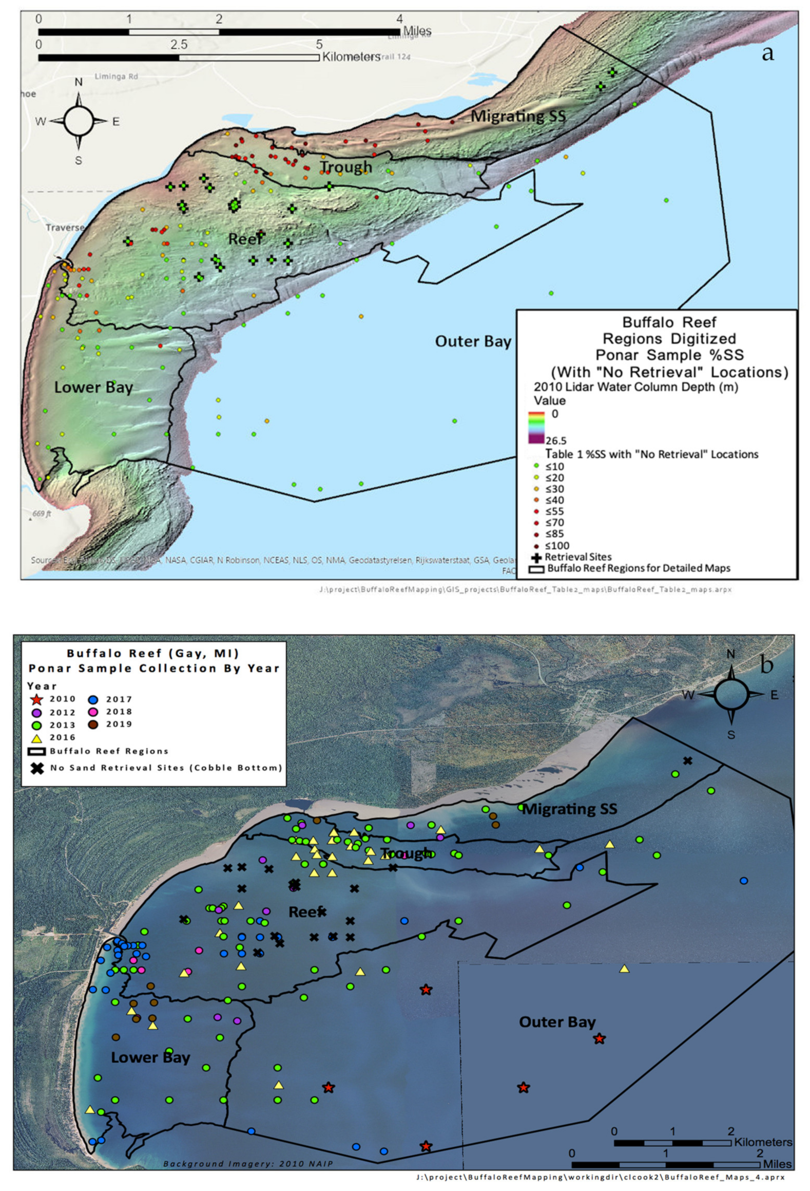
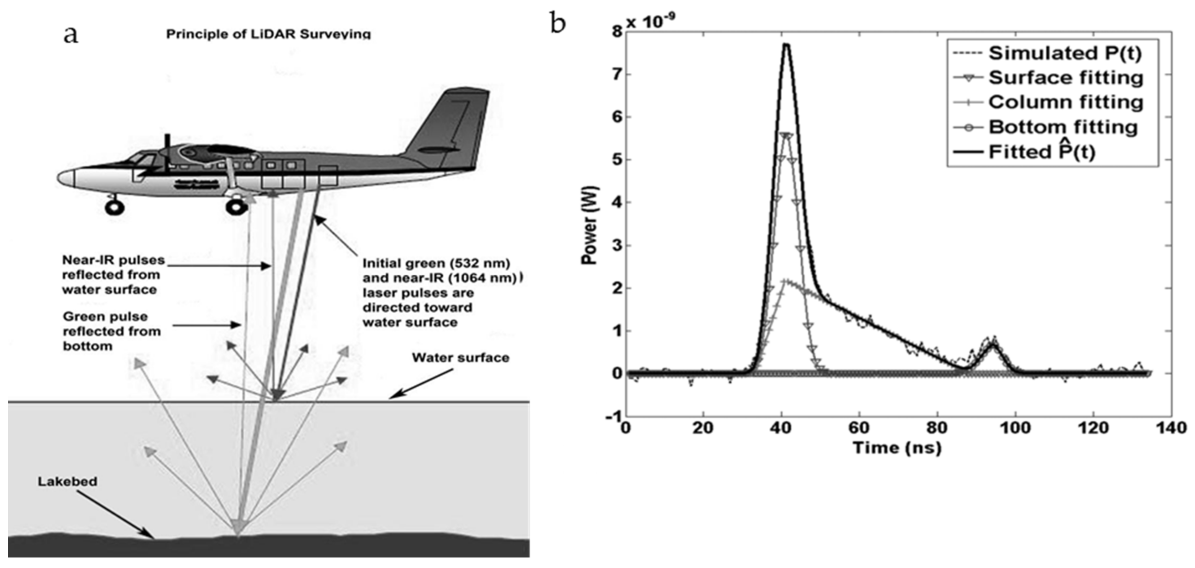
2.1. Obtaining LiDAR Information on Bay Substrates

LiDAR is an active remote sensing technique, used here in the ALS (airborne laser scanning) version, where an airborne laser-ranging system acquires high-resolution elevation and bathymetric data [20]. The Compact Hydrographic Airborne Rapid Total Survey (CHARTS) and the newer Coastal Zone Mapping and Imaging LiDAR (CZMIL) systems are integrated airborne sensor suites used to survey the coastal zone, in which bathymetric and terrestrial topographic LiDAR data are collected with aircraft-mounted lasers (Figure 5a,b; [21]). In coastal surveys, an aircraft flies over a water stretch at about 60 m s−1, pulsing two varying laser beams in sweeping fashion toward the Earth through an opening in the plane’s fuselage. The two lasers emit beams, an infrared wavelength beam that is largely absorbed by water, but strongly reflected off terrestrial features and a narrow, blue-green wavelength beam that penetrates the water surface and is reflected off the underwater substrate surface (Figure 5a). The LiDAR sensor records the time difference between the two signals (Figure 5b, waveform) to derive detailed measurements of bottom bathymetry. Quality control and editing were done in GeoCue’s LP360, bulk datum transformations with NOAA’s VDatum, then products were generated using Applied Imagery Quick Terrain Modeler and ESRI ArcGIS (ArcMap and ArcGIS Pro). Under ideal conditions in coastal waters, blue-green laser penetration allows the detection of bottom structures to a depth approximately three times passive light reflection. LiDAR achieves around 22 m penetration in Lake Superior [11] compared to 40 m in oceanic environments [22].
Along the coastal beach margins, elevation and spatial studies utilize a combination of periodic aerial photographs (including those of the National Agricultural Imagery Program, NAIP), and multiple LiDAR overflights, whereas underwater regions benefit from a combination of LiDAR/MSS, 3-band NAIP photography, ROV photography, and in situ Ponar sampling of substrates [11,12,13,15]. A major asset of LiDAR/MSS application is rapid, large-scale spatial characterization of the bay’s coastal zone elevation and bathymetry in different years, producing seamless land and water maps (e.g., Figure 3). However, the error associated with LiDAR DEMs (digital elevation/bathymetry models) is sensitive to several variables: mechanical collection (GPS coordinate system, scan altitude and speed, scan pattern, pulse-repetition rate, aircraft yaw and roll) and signal processing, weather, sea state, depth, water clarity, and wave-form clarity. Depth is important; for example, the horizontal and vertical accuracy of the CZMIL system has been described as 3.5 + 0.05 × d meters and [0.32 + (0.013 × d)2]1/2 m (Optech Manual), respectively, where d is the water depth. Details of resolution and accuracy in oceanic projects are discussed in Guenther et al. [25], Zhao et al. [26], and Yeu et al. [27]. With multiple instrument measurements, vertical LiDAR accuracy can be enhanced to 0.2m in shallow coastal waters [27], and can be as good as 0.22 (range 0.16–0.31) m along terrestrial strips [28]. In particular, under low-flying, high-density scanning characteristic of coastal and Great Lakes shorelines, horizontal resolution is listed by JALBTCX as 0.5–1.0 m (0.7 m) along inland beach environments, with vertical accuracy of 15 cm (Optech Manual; [29]). Spatial resolution decreases to ca. 2 m in deeper waters (10–20 m). Underwater DEMs are usually delivered with tiled 3 m resolution.
The geometry of DEMs permits many viewing options and cross-comparisons. DEMs can be statistically cross-compared with sonar bathymetry, or the vertical relief exaggerated to highlight specific bathymetric features (e.g., Buffalo Reef bedrock rises, ‘trough’ depressions). For example, statistical software packages (SYSTAT) were used to compare LiDAR-derived depths from 2008 with georegistered National Water Resources Institute (NWRI) sonar-derived depths (from Bieberhofer and Prokopec [30]). The resulting regression matches were very close (see Figure 4b in Kerfoot et al. [11]; R2= 0.98). Shadow techniques (hillside shading, or “hillshading”) can be applied to accentuate 3D features, whereas colors can be added to differentiate depth regimes (e.g., Figure 3). Later, we will rotate the viewing angle from nadir to nearly horizontal to examine various specific bathymetric features of Buffalo Reef and the coastal shelf. Moreover, because the available LiDAR simultaneously covers above-water (elevation) and below-water (bathymetry) environments, subtle beach features become evident. For example, in Figure 3, the nearshore shallow reaches of the natural sand beach in the southern bay and the stamp sand beach in the middle bay are different, the eastern migrating underwater stamp sand bars are very long and rope-like (disengaging from beach margins) as they move across bedrock, and the ancient riverbed channel stands out in clear relief.

2.2. Ponar Sampling (In Situ Measurements)

Bay sediments were sampled with two Ponar devices: a “Petite Ponar” and a “Standard Ponar”. The Standard Ponar grab is generally considered capable of efficiently sampling the widest variety of substrates, was designed specifically for Great Lakes sediment, and has been extensively evaluated [31,32]. Both devices were purchased from Wildco. The Standard Ponar weighed ca. 28 kg, with a surface area of ca. 0.05 m2, whereas the Petite Ponar sampled one-half the surface area, and weighed considerably less. See description below (Table 1), taken from Wildco listings.
The average bite depths of 70 versus 89cm would seem similar for sampling surface mixtures of sands. A single Standard Ponar grab (34′ R/V Agassiz) samples a larger surface area than the Petite Ponar grab, and is preferred for sampling benthic organisms. For % stamp sand determinations, we used both devices because there was no significant difference between the two devices in field tests (see below). However, there is a difference in efficiency. Often twice as many Petite Ponar samples can be taken as Standard Ponar samples in the same time [33]. Although we used both Standard Ponar and Petite Ponar for % stamp sand determinations, we preferred the Petite Ponar for rapid, shallow-water sampling of sand deposits off the smaller Michigan Technological boats (27′ R/V Osprey, 24′ R/V Polar), because more samples could be taken at less cost.
To check for any differences relative to %stamp sand determinations, we sampled sediments at 13 sites with both devices from the R/V Agassiz, over a range in stamp sand percentages of ca. 10–50%, then compared counts with a match regression analysis. Over the range, we found a very high correlation on percent stamp sand (% SS) between both devices (Multiple r = 0.944; regression equation Y = 1.020X + 0.461). The regression slope was not significantly different from zero (95% CL 0.78–1.25), with an intercept not significantly different from zero (SE = 3.98; p = 0.90; C.L. −8.3 to 9.2). That is, there was no significant difference between the Standard Ponar and Petite Ponar relative to measuring % SS in sand mixtures. Consequently, we do not distinguish Petite from Standard Ponar origin in the % SS table (Supplementary Table S1). Over a span of 10 years (2010–2019), a total of around 175 Ponar samples were taken from Grand (Big) Traverse Bay (Figure 6a,b). Subsamples were taken during the past two years from collection bags and counted for the % SS determinations shown here. Only Standard Ponar grabs were used to sample benthic organisms, for we wanted the greatest number of individuals in species and diversity determinations. Because of this, the number of macroinvertebrate taxa sites sampled was lower, only ca. 80, and was dominated by 2013 sampling (Figure 6b).

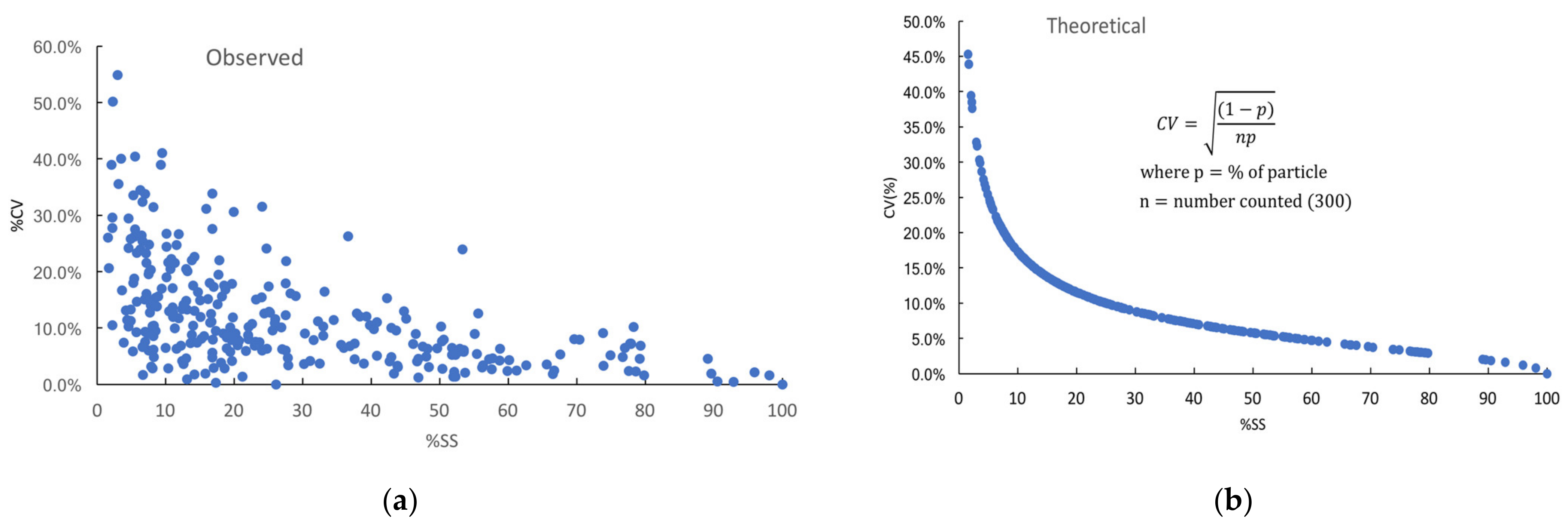
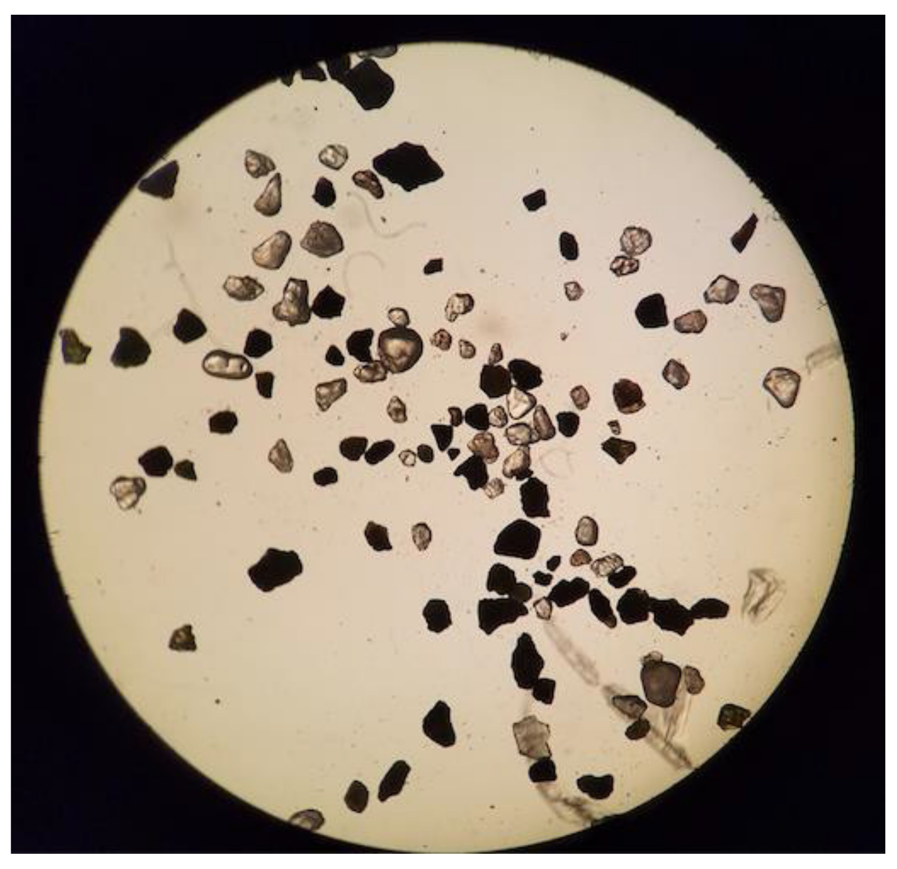
2.3. Determination of Stamp Sand Percentages in Sand Grain Mixtures

Across the coastal shelf, a major novel challenge was determining the percentage of stamp sands in mixtures of stamp sands and natural sands. Early studies by Bieberhoffer and Prokopek [30] utilized largely standard sonar transects to determine substrate types. The studies were important for clearly defining the boundaries of “Buffalo Reef” and for mapping sand fields, cobble, and bedrock substrates. However, sonar failed to differentiate stamp sands from natural sands because grain sizes in sediments were often very similar. Our MSS studies were the first to map stamp sand substrates, but encountered numerous bottom reflectance complications [11,13,14].
However, the two principle sand types in the bay come from distinctly different end-members. The crushed Portage Lake Volcanics, the so-called “stamp sands”, are basalts (K, Fe, Mg plagioclase silicates; augite, and minor olivine), whereas erosion of the coastal bedrock (Jacobsville Sandstone) releases rounded quartz sands that make up the white beach sands. We discovered that, under a microscope (Olympus LMS225R, 40–80×), particle grains from the 2010–2019 Ponar samplings could be separated into crushed opaque (dark) basalt versus rounded, transparent quartz grain components (Figure 7), allowing calculation of % stamp sand particles in particle (sand) mixtures. Percentage stamp sand values were based on means of randomly selected subsamples, with 3–4 replicate counts, around 300 total grains in each sub-count (Supplementary Table S1). Standard deviations and errors were calculated for individual samples and the means used to calculate confidence intervals for typical counts. For example, for 108 initial sites, the mean 95% confidence interval was around ±4.5%.
Counts of the two mixed grains generally followed a binomial distribution, where there was an inverse relationship between the coefficient of variation (CV = SD/mean) and the mean % stamp sand (Figure 8a,b). That is, if the mean % stamp sand was high (>50%), the Coefficient of Variation (CV = SD/mean) was relatively low (3.1%, N=12), but if the mean was < 10%, the CV was much higher (mean = 25.3%, N = 30). Examining the 10 years of samples, we found a good agreement between measured (Figure 8a), and expected CVs from a binomial distribution (Figure 8b). Sub-tallies, means, and CVs for individual counts are included in Supplementary Table S1.

2.4. Manganese Grain Correction

Small numbers of natural manganese grains were found in both beach and underwater sands. The inadvertent inclusion (misidentification) of natural manganese sands [34] as stamp sands, although relatively scarce in underwater bay sediments, could influence low-end calculations of % stamp sand in grain mixtures. Manganese grains occur in sporadic patches along beach sands, occasionally reaching as high as 32% of grain counts (Supplementary Table S2). In the laboratory, we found that under the microscope, reflected light could be used to distinguish natural manganese sand (grey metallic color, opaque) from stamp sand basalt particles (dark brown, greenish, opaque), easily differentiating the two particle types. Manganese grain percentages ended up relatively low in underwater sand samples, on the average only making up around 1.8% of grain counts. Nevertheless, we assayed both beach sands and underwater sand samples for manganese grains, and corrected initial percentage stamp sand counts (Supplementary Table S2).

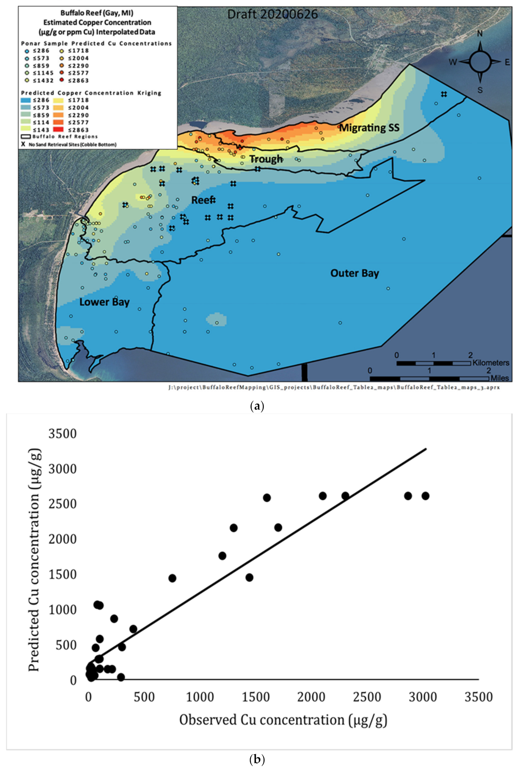
2.5. Cu Concentrations: Predictions from % SS Versus Directly Assayed Samples

If copper concentrations remained constant in tailings grains dispersed across the bay, we could use extensive Gay pile determinations (see below, N = 274, mean 2,850 ppm Cu) to predict concentrations of Cu in stamp sand/natural sand mixtures. For example, a mixture of 50% stamp sand would predict a Cu concentration of 1432 ppm (50% stamp sand × 2863 ppm = 1432 ppm Cu). Once the % SS was determined for bay samples, the predicted Cu concentration could also be listed (Supplementary Table S1).
Direct assays of stamp sand metal composition from the Gay Pile have been done using several methods, showing relatively high copper concentrations plus a Supplemental suite of secondary metal concentrations (Neutron Activation and ICP Mass Spectrometry [4,35,36]; ICP Mass Spectrometry [37,38]). Early studies of Cu concentrations in the Gay pile’s coarse stamp sand found values ranging between 1620–5486 µg/g (mean 2697 µg/g, n=7 [4,6]), whereas the more numerous sampling studies by MDEQ on the Gay tailings pile [37] found Cu concentrations 1500–13,000 µg/g with a mean of 2863 µg/g; n=274). Thus, we used the MDEQ mean as the standard. In the MDEQ sampling, metal concentrations from the secondary suite at the main Gay pile also averaged concentrations of: Ag 0.4–7.7 µg/g (mean 1.8), As 1.0–15.5 µg/g (mean 1.5), Cr 18–52 µg/g (mean 28.8), Co 16–36 µg/g (mean 22.9), Hg 0.06–0.11 µg/g (mean 0.027), Ni 20–48 µg/g (mean 31), Pb 5.1–6.1 µg/g (mean 2.6), and Zn 48–120 µg/g (mean 74.7) [37]. From studies at the EPA Duluth Lab, copper was found to be the primary toxic element in stamp sands [39,40], so here we only emphasize effects of copper.
To check the % stamp sand-predicted Cu concentrations directly against observed Cu concentrations, we determined Cu concentrations directly on several Ponar samples, constructing a “calibration curve” (see preliminary results in [15]). For direct Cu determinations, Ponar sediments were digested at MTU in a microwave (CEM MDS-2100) using EPA method 3051A. Solutions were shipped to White Water Associates Laboratory for final analysis. Copper was measured using a Perkin-Elmer model 3100 spectrophotometer. Digestion efficiencies were verified using NIST standard reference material Buffalo River Sediments (SRM 2704), and instrument calibration was checked using the Plasma-Pure standard from Leeman Labs, Inc. Digestion efficiencies averaged 104%, and the calibration standard was, on average, measured as 101% of the certified value. Despite minor deviations at both high and low ends of the index, there was a very good overall fit between % stamp sand-predicted Cu concentration and directly measured Cu concentrations (see preliminary regression, R2 = 0.911, in [15]). However, the “calibration curve” regression did show a non-zero intercept, indicating that predicted values were higher than observed values. To check the original calibration curve, we doubled the number of observed Cu assays to around 40 and ran the regression again, which we present here. We originally attributed the non-zero intercept to naturally occurring manganese sands in samples near the low end of “stamp sand” percentages. Now we also suspect that stamp sands closer to the original Gay pile have slightly higher Cu concentrations, whereas stamp sands around the Traverse River Seawall, and in the lower and outer bay regions, have lower relative Cu concentrations.

2.6. Benthic Invertebrate Surveys

Eighty of the 175 Ponar samples, largely from 2013, were checked for benthic invertebrate community (macro-invertebrate) composition and diversity, and compared with stamp sand percentages. Site sampling for sediment and benthic organisms included three cruises in August 2012, two cruises in May 2013, and three cruises in June 2013. The final later cruises were in September and October of 2016, and spring of 2017. Complementary activities included side-scan and down-scan sonar, and remotely operated underwater vehicle (ROV) underwater filming at 17 sites. Benthic invertebrates were washed in a sediment elutriator and filtered through 350 μm mesh. Organisms were preserved in 10% formalin sucrose and kept in cold storage until identified in the laboratory. Taxa were identified and enumerated under a dissecting microscope using identification keys by Pennak [41] and Thorpe and Covich [42]. The benthic community data can be treated in multiple ways relative to measures of % stamp sand: (1) regression plots of taxa (species) density versus % stamp sand, or (2) regression plots of species richness and diversity (Shannon–Weiner index) versus % stamp sand. For this effort, we recounted samples and increased taxa from six to eight categories (Supplementary Table S3). Both linear and non-linear regressions were fitted to density and diversity trends. However, we mapped only total benthic density patterns across the bay. These are the first spatial maps of benthic density depression for the bay. Individual species counts can be found in Supplementary Table S3.

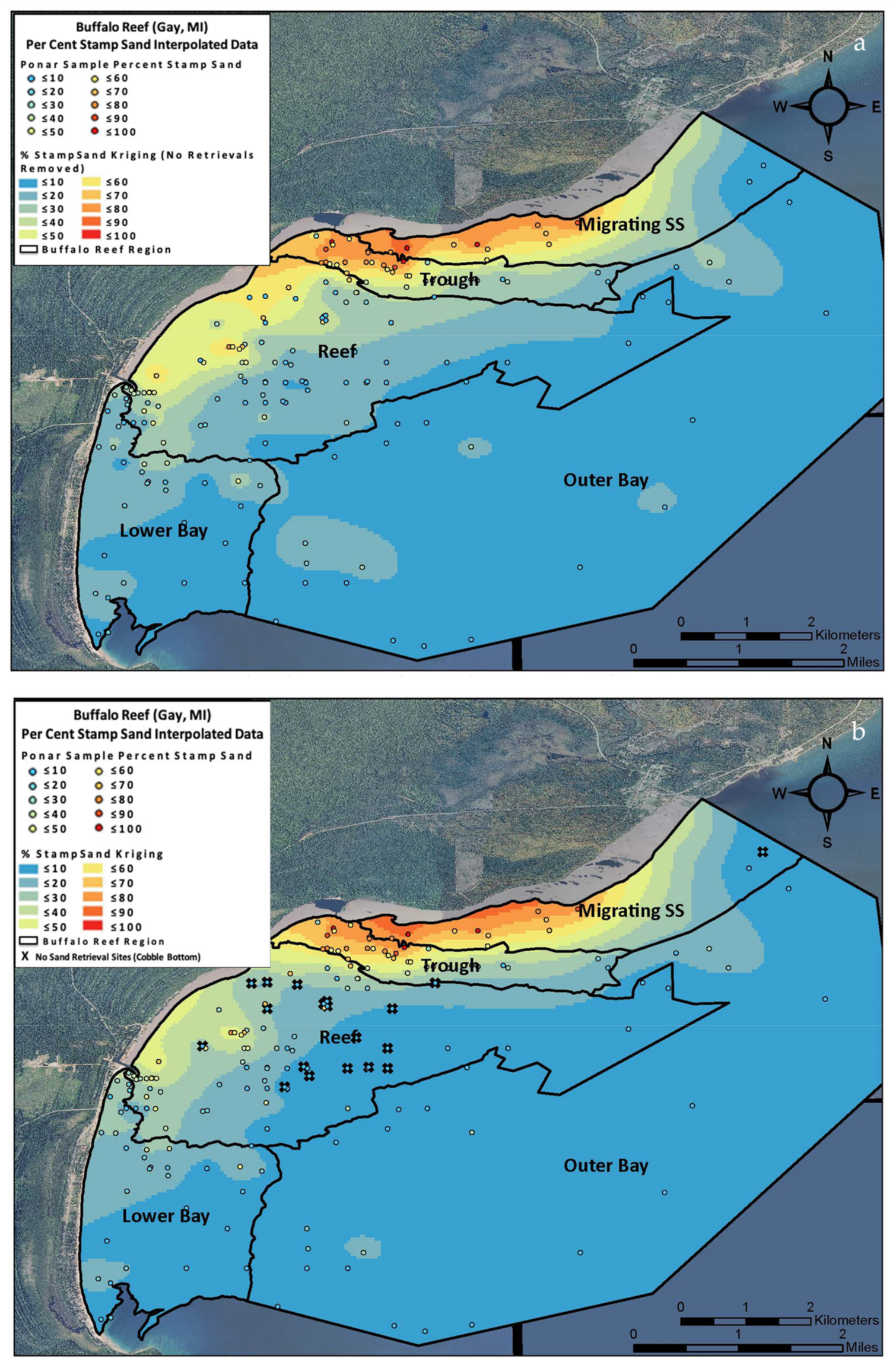
2.7. Map Construction Techniques

For sediment characteristics (percent stamp sand and estimated copper concentration), interpolated maps were generated using a kernel density estimation approach that accounted for some physical barriers to movement posed by elevation differences along the coastal shelf (LiDAR), particularly the ancient riverbed (the ‘trough’) that has captured much of the underwater migrating sands. Interpolation was performed using the “Kernel Interpolation with Barriers” tool available from the Geostatistical Analyst toolbox in ArcGIS Pro 2.5 (ESRI, Redlands, CA). This tool interpolates a surface between sample locations using the shortest distance between points without intersecting the barrier, allowing the contour to change abruptly at the edge of the barrier [43]. At the extreme, contouring could be applied that recognized the five boundary regions (see later in Discussion) or interior bathymetric layers, such as bedrock relief along the midrib of the reef. Barriers were utilized with variable constraints (examples ranging from weak barriers to strong barriers). Here, in final maps, we mainly present examples that have minimal barriers constraints. Minimal barriers allowed application of contouring to as many points as possible across the bay. However, extreme cases ranging to strong barriers were also examined. An example is given in the Discussion. Our anticipation is that use of “Barrier” algorithms will eventually interface with detailed hydrodynamic modeling of particle transport [13,15,19].
However, Ponar non-retrieval of sand mixtures over regions of bedrock or cobble/boulder pavement, especially along rises on Buffalo Reef, also posed a potential problem to accurate geospatial analysis. In these circumstances, the Ponar would bounce off of bedrock or cobble pavements, without retrieving sediment. Therefore, we ran alternative contouring scenarios, and present one situation without “non-retrieval” sites and another situation that incorporated “non-retrieval sites”. In “non-retrieval” cases, we assigned zero values for stamp sand percentage. Both those cases are presented in the Results section.
The key user-defined parameters for the “kernel interpolation with barriers” tool were the kernel function, the bandwidth value, and the search neighborhood characteristics. The kernel function was set to exponential and the bandwidth to 0.02 (the power and ridge parameters retained their default values of 1 and 50, respectively). The bandwidth is a smoothing value that determines the width of the kernel. Here, the bandwidth value was chosen based on a combination of visual inspection (running successive trials and selecting the estimate that was most in accordance with our prior knowledge about bathymetry and sediment transport patterns [19,44]) and the RMSE from the cross-validation diagnostics. Finally, a smooth circular search neighborhood was utilized with a smoothing factor of 0.5 and a radius of 0.1.
Macroinvertebrate density, for which elevation differences do not necessarily represent physical barriers, was interpolated using an empirical Bayesian kriging (EBK) method. EBK is advantageous over other classical kriging methods because it estimates error in the model by accounting for multiple semivariograms versus a single semivariogram [45]. An exponential transformation was applied and the semivariogram model was set to K-Bessel detrended, a processing-intensive but robust modeling approach. The first-order trend in the case of macroinvertebrate density is the general northwest–southeast gradient, with low densities (most impacted) along the migrating stamp sands and adjacent trough and higher values (least impacted) further south and east into the bay.

3. Results

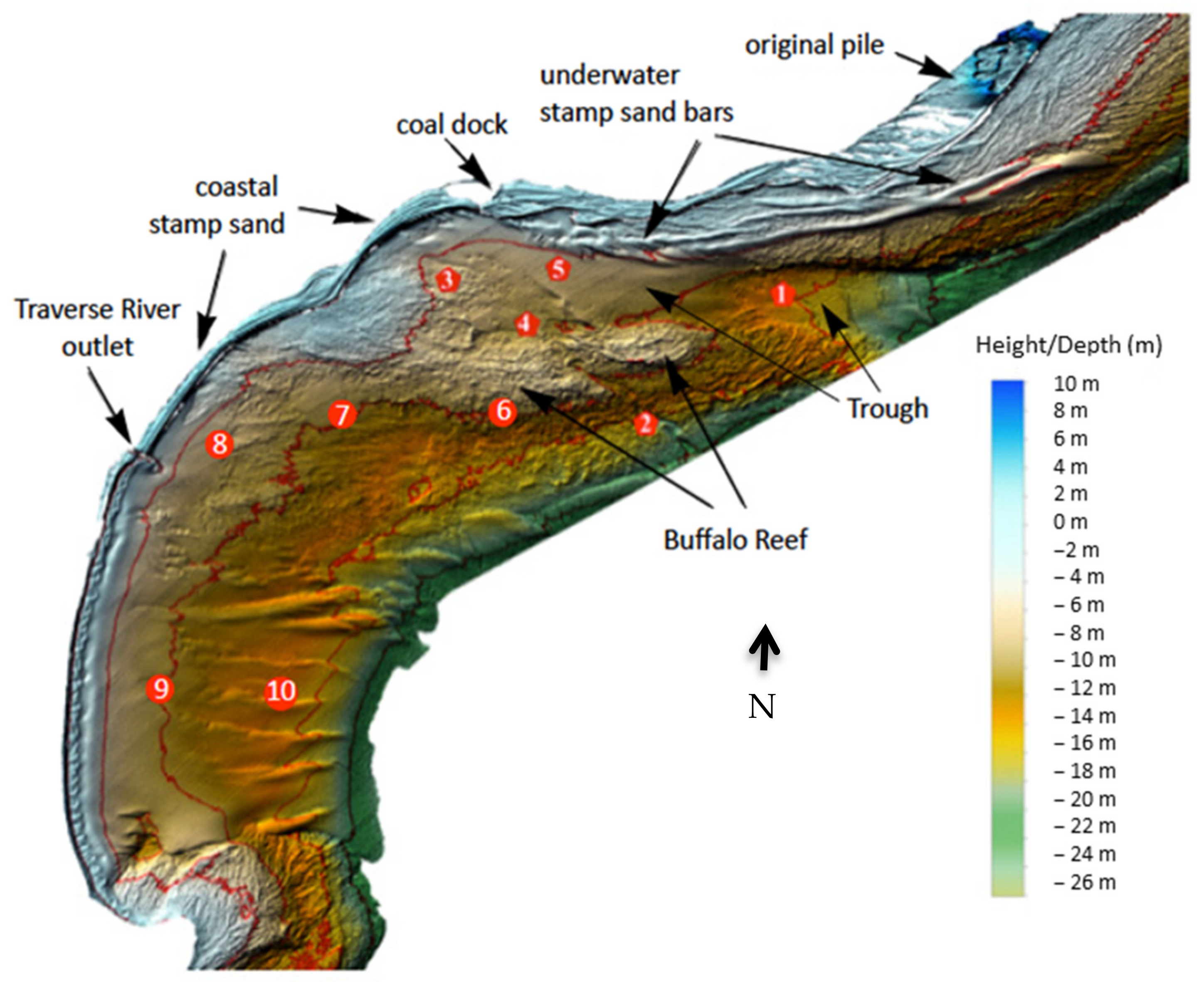
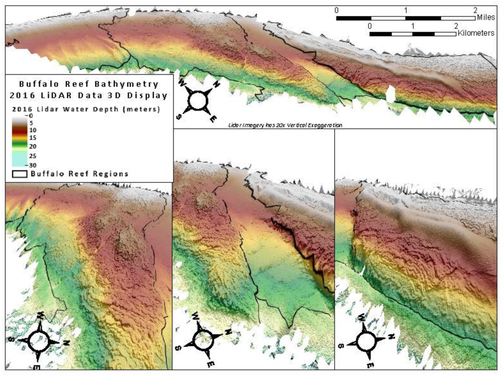
3.1. Non-Nadir LiDAR Bathymetry

One advantage of using DEMs created from LiDAR point clouds is that they can be vertically exaggerated to accentuate known features or barriers. Recall that Figure 3 illustrates the standard nadir (overhead) view of Grand (Big) Traverse Bay as captured in a 2010 LiDAR-derived DEM. In contrast, Figure 9 shows how features from the 2016 LiDAR-derived DEM can be emphasized by exaggerating the vertical scale by a factor of 20, allowing the viewer to see subtle changes in bathymetry. Viewing rises and depressions from a largely horizontal (ca. 15°) angle, and allowing for overlay of elevation and solar-azimuth shading data, helps the viewer interpret the potential impact of natural environmental 3D barriers on sand advection and deposition. LiDAR bathymetry was initially used by Hayter et al. [19] to help model SS deposition on Buffalo Reef [13]. In Figure 9, we emphasize how the hillshaded DEM captures the coastal shelf region, the elevated and interrupted bedrock ridges of Buffalo Reef, the ancient river cut north of Buffalo Reef (‘trough’), and the eastern migrating bars of stamp sands that move across the Jacobsville Sandstone bedrock. The rope-like migrating bars detach from the shoreline region of the original Gay pile and the redeposited stamp sand beach between the original pile and the historic Coal Dock. Notice how the relative smoothness of the migrating stamp sands contrasts with the bedding irregularities of Jacobsville Sandstone bedrock. Underwater migrating stamp sand bars appear mainly to be moving into the northern reaches of the ancient riverbed, whereas the end of one southern bar appears to be descending along the shelf scarp, eventually to move into deeper waters.

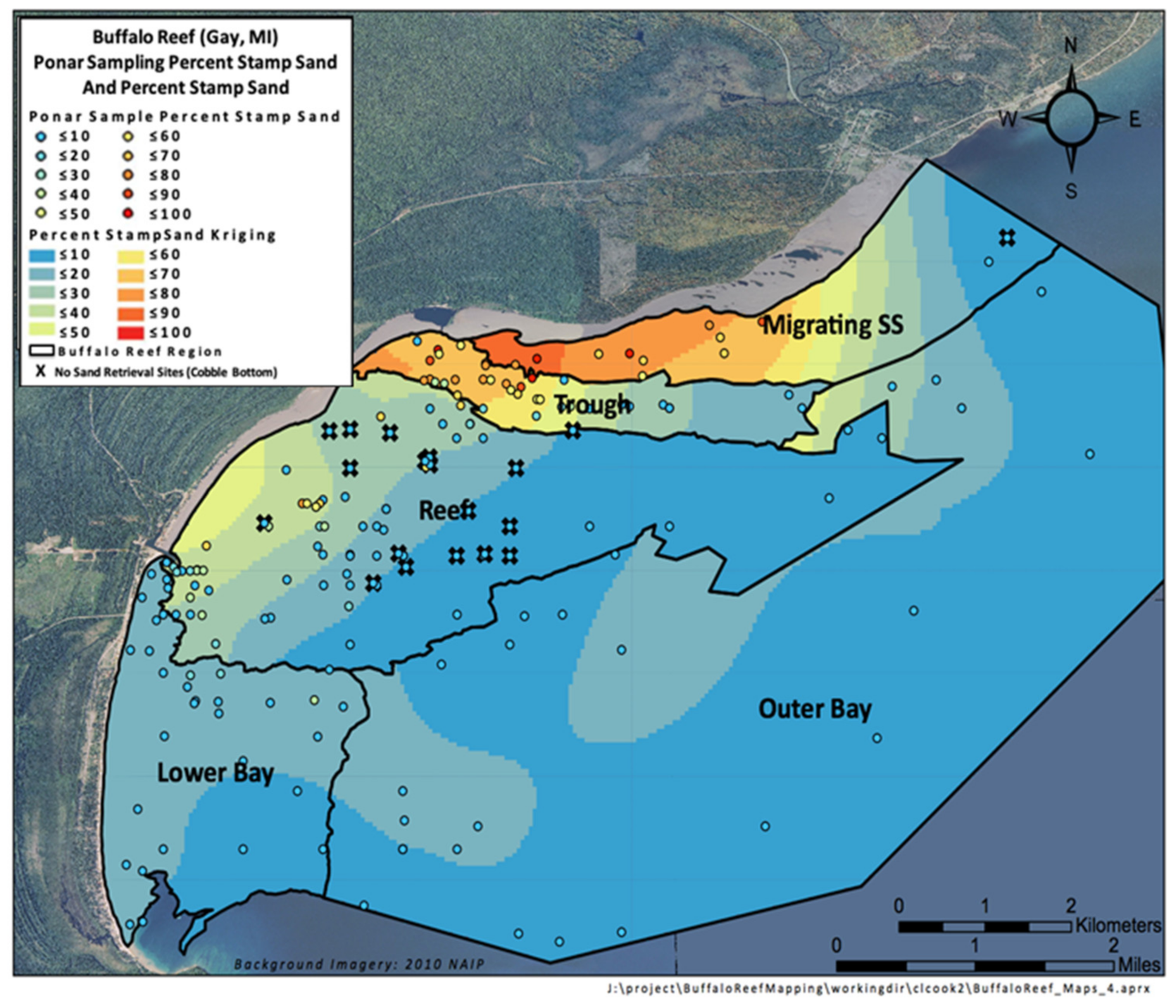
3.2. Determining Percentages of Stamp Sand in Sand Mixtures Across the Bay

As mentioned earlier (Methods), because the sources of sands are so distinct (crushed opaque basalt, from the Portage Lake Volcanic deposit; versus rounded, clear quartz from eroding Jacobsville Sandstone), stamp sand grain percentages could be determined directly from Ponar grain counts. However, as the Ponar dredge only penetrates around 6–8 cm deep, the percentage stamp sand values are largely surface measurements. Stamp sand percentages from ca. 175 underwater sites are plotted and color-coded in Figure 10a,b (see legends). Specific site values are listed in Supplementary Table S1. Stamp sand percentages are contoured, and the contours color-coded (lower legend, upper left). When percentage stamp sand is contoured across the bay, there are distinct geospatial patterns. Stamp sand percentages are highest (70–100%) in near-shore waters between the original Gay tailings pile and the Coal Dock, moving off the stamp sand beach and into the northern reaches of the ‘trough’. High values extend out around 1 km. High percentages include samples from the migrating underwater bars, which separate off the eroding Gay pile and stamp sand beach shoreline [13,14]. Underwater percentages decline westward towards the Traverse River Seawall, down to 50–60% SS. Values are highest again immediately off the stamp sand beach. At the Traverse River Harbor, tailings are accumulating both along the beach (Figure 4c,d) and underwater offshore (Figure 10). Stamp sand is backing up along the coast behind the Seawall, periodically over-topping (Figure 4d). There is also stamp sand accumulating in a bathymetric depression (so-called ‘eye’ of Buffalo Reef, Figure 3 no. 7). LiDAR bathymetry suggests stamp sands from the Seawall field are dropping down into the ‘eye’ depression through ridges, creating a small field (Figure 9 and Figure 10). Stamp sands are moving offshore around the Traverse River Seawall and into the Lower Bay (Figure 10a,b).
The elevated rock ridges of Buffalo Reef have less stamp sand (20–30% SS) and there are very low values (<10% SS) along the southern margin of the mid-rib bedrock field. Thus, the maps show that stamp sand is not yet moving down the ancient riverbed (‘trough’) enough to curl around the rugged southern bedrock margins (Figure 9) of Buffalo Reef. However, stamp sand could be moving southward into the lower bay from the Traverse River over-topping and eastward and southward from the ‘eye’ location (Figure 10a,b). Thus, stamp sand is encroaching from both eastern and western sides onto Buffalo Reef. The % SS maps also provide important information about how much area of Buffalo Reef is covered by stamp sands. Sand fields with a 40% mix of SS cover around 16–18% the surface of Buffalo Reef. Earlier estimates, using a variety of techniques (bottom reflectance, initial Ponar sampling; see Discussion and Kerfoot et al. [13,15]), estimated stamp sands covered ca. 25–35% of Buffalo Reef in 2009–2016, but did not give percentages of stamp sand. However, in addition to periodic ‘over-topping’ of the Seawall into the Traverse River (Figure 4c), the movement of SS around the Traverse Harbor Seawall and into the lower sand bay threatens an important rearing ground for lake whitefish (Coregonus clupeaformis). Once lake whitefish hatch on Buffalo Reef, they move into the lower bay. Scattered values above 10% SS are also evident in the lower bay and sporadically appear offshore in the outer bay. In Figure 10b, ‘non-retrieval’ sites, essentially locations where the Ponar bounced off bedrock and pavement surfaces, are assigned a 0 value for stamp sands. This alters the contouring slightly, as stamp sand cover on Buffalo reef is lessened and values dip in more towards the shoreline where the Buffalo Reef rise intersects the shoreline.

3.3. Sediment Copper Concentrations: Values Predicted from % Stamp Sand Compared with Direct Assays (Regression Analysis)

In Grand (Big) Traverse Bay, since the Gay tailings pile was the principal source of stamp sands, we used copper concentrations from this source to determine a standard (see Methods). The MDEQ values (i.e., 100% stamp sands = 2863 μg/g) were used to predict Cu concentration based on % stamp sand in mixtures across the bay. Predictions of Cu concentrations based on % stamp sand calculations assume no differential sorting of Cu-rich particles by wave action, either by grain size or specific gravity. Supplementary Table S1 gives the predicted Cu concentrations from %stamp sand counts for 175 sites. As a check on % stamp sand-predicted Cu concentrations, we directly analyzed Cu concentrations in many Ponar samples, then constructed a “calibration curve” (regression method) which compared predicted versus observed Cu concentrations for 40 sites. Cross-comparisons with these regression results suggested relatively lower Cu values in the ‘lower’ and ‘outer’ bay regions, beyond mere adjustments for Mn grains, so we lowered Cu concentrations in these regions.
Spatial contours for copper concentrations are given in Figure 11. At first glance, there appears to be high correspondence between the % stamp sand maps (Figure 10a,b) and the Cu concentration map (Figure 11a). This similarity is to be expected, because Cu concentrations were initially predicted from % stamp sand (Supplementary Table S1), since stamp sands were the primary source of Cu. However, when Cu concentrations (x-axis) from Ponar samples were directly assayed and plotted versus predicted Cu concentrations (derived from % stamp sand, y-axis), the regression had some interesting properties. There was a highly significant linear fit (Figure 11b; Y = 1.010X + 219.9; F(1,39) = 250.2, p = 2.64x × E-18; R2 = 0.868). The correlation between observed and predicted values (r = 0.932) was good, but with some scatter (SE = 337). Notice also that the slope of the copper calibration regression (1.010X (SE = ±0.064, t = 15.8) was close to 1.00, which was also encouraging. However, there was again a slight, significant displacement of the regression line Y intercept value from zero (+214 µg/g, SE = ±62.9, t = 3.41, p = 0.002). Moreover, the intercept 95% C.L. (87 to 342) did not include the origin. Two possibilities, mentioned earlier, were considered: 1) natural manganese sand might have been erroneously tabulated as stamp sand in microscope counts, so that predicted Cu concentration was erroneously slightly over-estimated, or 2) Cu associated with particles was spatially sorted, with Cu more abundant in grains near the original pile and less abundant near the Traverse River, ‘lower’ and ‘outer’ bays. Both these options were checked, as we counted manganese grains in samples and made corrections (see Regression equation) after assaying the 40 sites directly for Cu concentrations (Figure 11b).
Cu concentrations in the coastal nearshore zone off the Gay pile to the Coal Dock region were very high (1432–2863 µg/g). High values extended out about 1 km into the upper regions of the ‘trough’. In the regression, observed concentrations closely matched predicted concentrations from the Gay pile standard (Figure 11b). Two km off the shoreline in a region between the pile and Coal Dock, Cu concentrations still ranged between 573–1432 ppm. However, western copper concentrations, past the bedrock ridge of Buffalo Reef (see Ponar non-retrieval sites, bold squares) and extending to the Traverse River Seawall, were relatively lower than expected, falling only in the range 859–1718 µg/g. On shore, in stamp sand next to the Traverse River Seawall, copper concentrations determined by MDEQ [37] were also lower, 710–5300 µg/g (mean=1443 µg/g; n=24), than values at the Gay stamp sand pile (mean = 2863 µg/g, n=274). Moreover, Zanko et al. [38] also found copper concentrations lower at the Traverse River (coarse fraction, 1210 µg/g) than at the pile (3420 µg/g). Therefore, in addition to manganese sands reducing Cu concentrations slightly as an artifact near the low end of values (Supplementary Table S2), there is evidence that particles from near the original Gay tailings pile contain higher concentrations of Cu than those from the Traverse River region, ‘lower’ and ‘outer’ bays. The latter phenomenon suggests differential dispersal of particles related to density (Cu concentration), at least over the bay range of 10 km. If nearshore stamp sands originate from shoreline sources around the Traverse River Seawall, reduction of Cu in particles at the Traverse River Seawall contributes to the observed 50% reduction of Cu concentrations per mass in underwater stamp sand off the Traverse River Seawall site.
Given the nearshore concentrations between the Gay pile and Coal Dock, biotic communities should be severely impacted. The high concentrations predict severe effects on benthic organisms (periphyton, invertebrates, larval fish) in the nearshore zone and underscore the peril to Buffalo Reef if the high concentration sediments in the Coal Dock Region transgress into boulder fields. At concentrations of 500–1500 µg/g (ppm), copper in sediments is likely to have toxic effects [9,10,46]. Caution is warranted, for 4 km off the shoreline, in deeper waters, there might be ameliorating effects from higher organic complexation. Although Cu concentrations greatly exceed EPA and Michigan probable effects levels (149 ug/g; [47]), organic complexation must be taken into consideration along the shoreline and in finer offshore sediments, partly because river discharges carry humic-stained waters (Figure 4d) and offshore sediments have higher carbon concentrations.

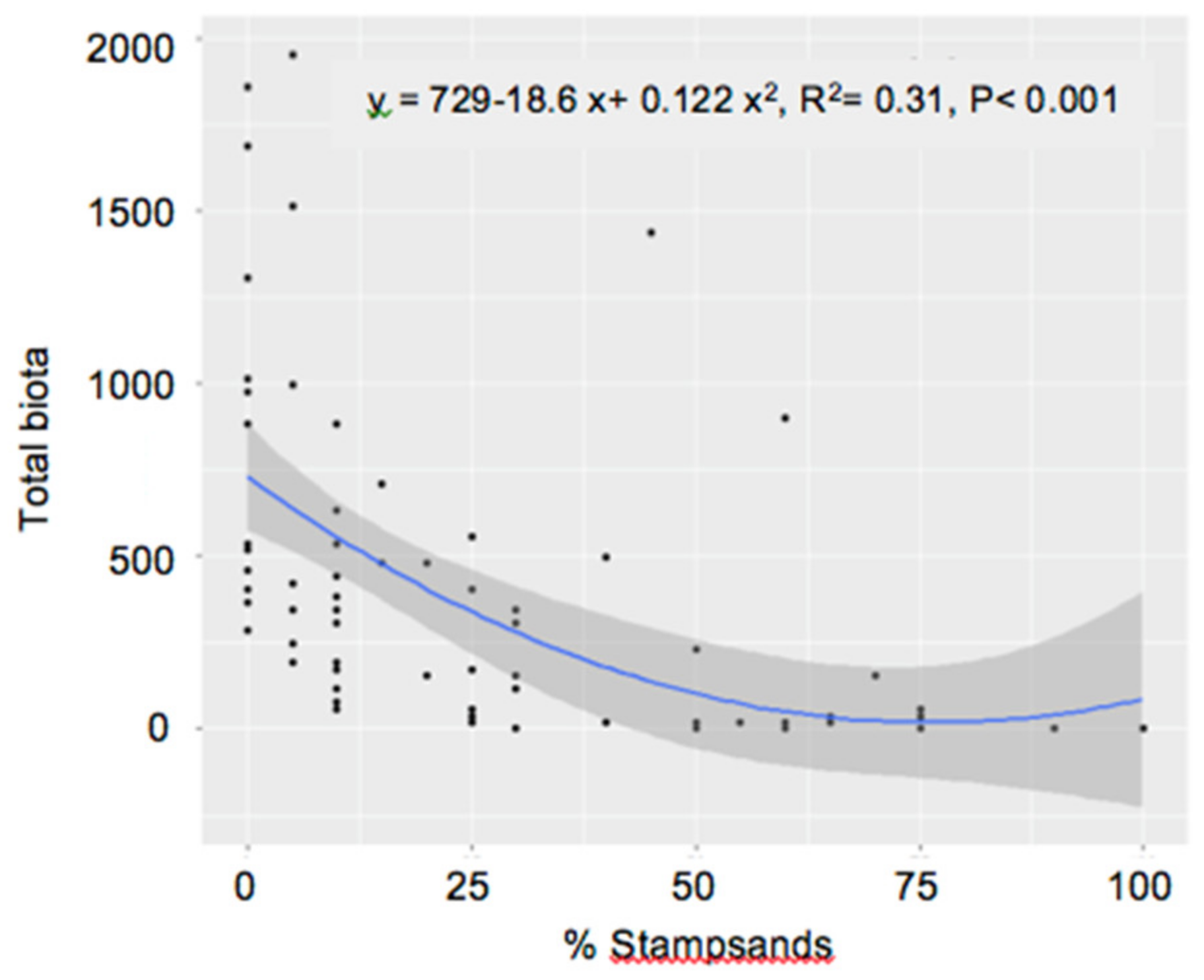
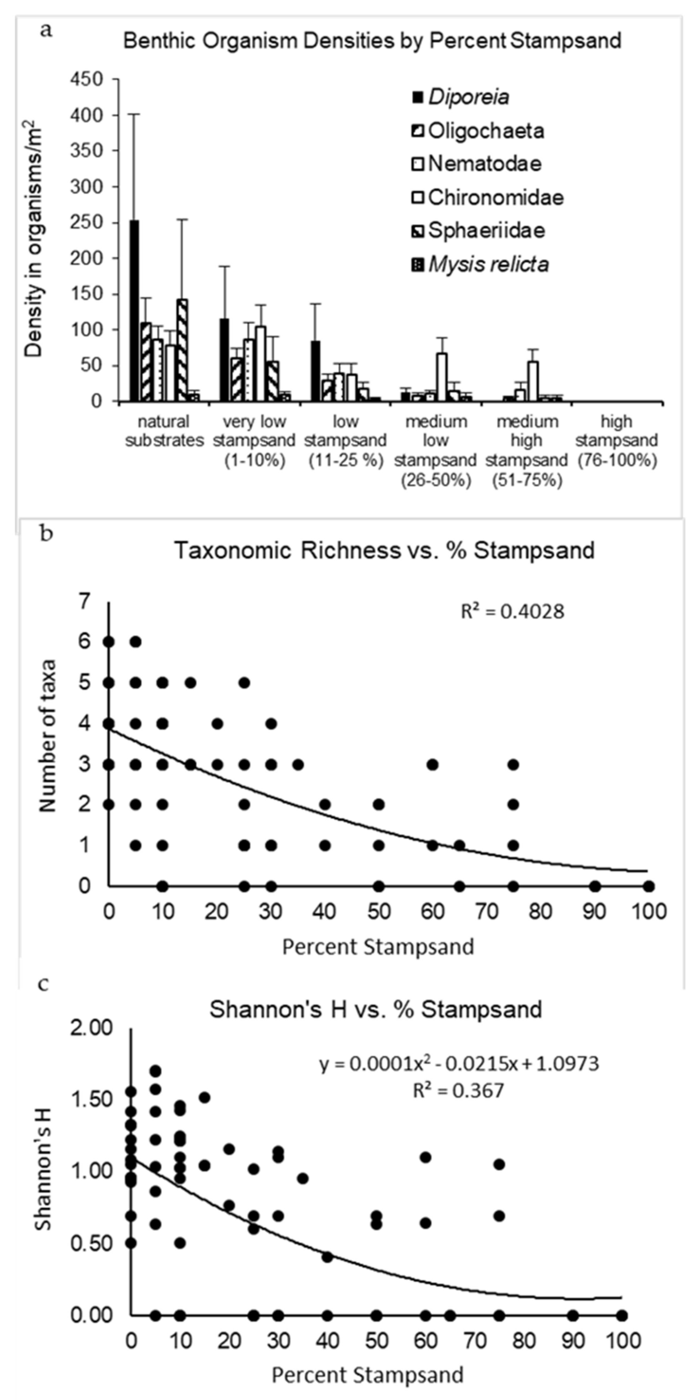
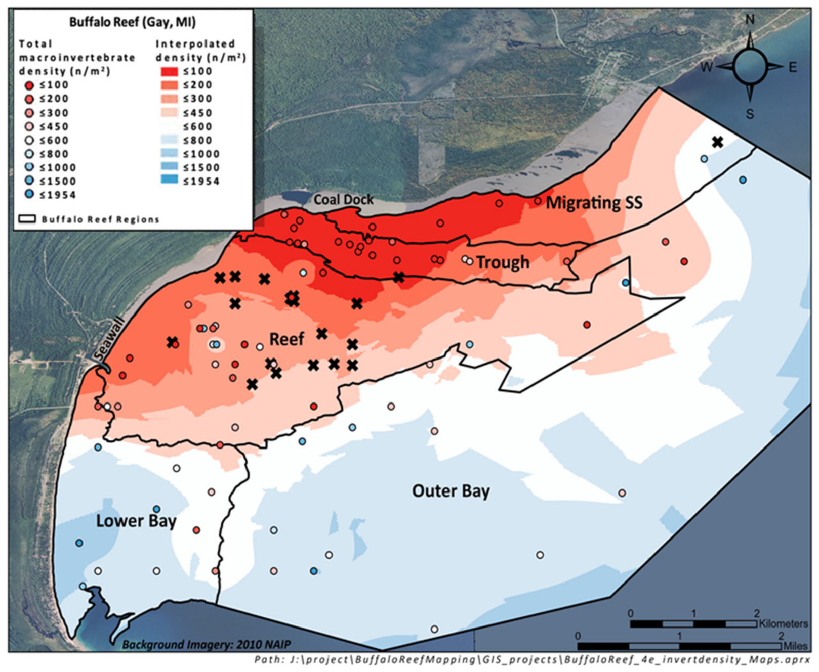
3.4. Benthic Invertebrate Community Survey

When percentage stamp sand is translated into copper concentrations, e.g., 100% stamp sand set at ca. 2863 µg/g copper, spatial toxic effects on biota would be expected, especially at observed high shoreline percentages (Figure 11a). Copper concentrations diminish as one moves away from the shoreline progressively into deeper shelf regions. Yet even at 1 km offshore, copper concentrations still fall within 1145–1716 µg/g (ppm). At these levels, copper is likely to have some toxic effects [9,15,39,40]. Direct laboratory tests of Gay stamp sand shoreline sediments on benthic invertebrates by Weston [37] and MDEQ [48] both showed toxic effects. ROV studies during 2012–2017 verified concerns about two separate processes: (1) physical drift of stamp sands into cobble fields, filling up crevices and “drowning” boulder fields [11,49]; and (2) potential toxic effects of migrating stamp sand on benthic organisms, including periphyton (diatoms and bacteria) on rocks, and benthic invertebrates [12,13,15]. Direct counts of invertebrates from Ponar sampling (Figure 12a and Figure 13) demonstrated severe effects on benthic species abundance and diversity at high concentrations of stamp sands (see preliminary discussion in Kerfoot et al. [15]), but macroinvertebrate effects were not spatially mapped until now. Benthic taxa that showed effects were numerous, across all 6–8 tabulated taxonomic categories (six taxa in Figure 12a; eight taxa in Supplementary Table S3). Lowest densities of benthic species were found near the shoreline between the Gay pile and Coal Dock (Figure 14). Above 26% stamp sand (ca. 600 µg/g), almost all taxa showed severe density depression. Above 75% stamp sand concentration (ca. 2100 µg/g), there were almost no observed organisms (Figure 12a and Figure 13). Although 95% C.L. are shown for individual taxa in Figure 12a, group quantitative measures of community variables associated with % stamp sand also confirmed statistical effects (Figure 12b,c). ANOVA on total benthic invertebrate densities revealed progressive effects in three statistically different data groups.
In Figure 12a, samples containing 0–10% stamp sand were statistically different from those containing 11–75% stamp sand (F = 7.2, p =0.014), which were statistically different from the >75% stamp sand category (F = 11.0, p = 0.003). A second degree polynomial fit to total macroinvertebrate density (Figure 13, R2 = 0.31, p< 0.001) shows a clear non-linear decline with increasing percentages of stamp sand. Species Richness (Figure 12b, R2 = 0.403; p < 0.001) and bio-diversity indices (Figure 12c, Shannon’s H, R2 = 0.367; p < 0.05) also showed significant non-linear declines with increasing stamp sands, reinforcing the interpretation of progressive impacts of stamp sand on benthic taxa around Buffalo Reef. Equations for all fit second-order polynomial regressions are given in Table 2.
Total macroinvertebrate densities in Grand (Big) Traverse Bay are plotted spatially in Figure 14 and contoured by kriging ArcGIS techniques (see Methods). Here low densities are in red, increasing through pinks to white and blues. Lowest density values (deep reds, upper left legend) are evident along stamp sand beach margins from the Gay pile to the Coal Dock. Densities increase a bit towards the Traverse River region and are higher in the middle and outer regions of Buffalo Reef. Densities in the Lower Bay and Outer Bay Control Regions are more normal. Densities in the Lower Bay served as “Control” values, the “natural substrate” values in Figure 12a. Notice that macroinvertebrate densities seem broadly depressed over much of Buffalo Reef. Density effects on macroinvertebrates appear spatially more widespread than the spatial patterns for stamp sand percentages or copper concentrations. Effects extend across larger areas of Buffalo Reef, indicating that 80–90% of the area is affected. Clearly the shoreline adjacent to stamp sand beaches is highly compromised, and effects continue into northern, northeastern, and western boundary regions of Buffalo Reef.
Tallies for the eight separate macroinvertebrate taxa counted at each site versus % SS (Supplementary Table S3) were also compared. If simple linear correlation coefficients are run on total density versus % SS, the correlation coefficient is −0.510 (for N = 79, a highly significant inverse relationship; p < 0.001). Recall that second polynomial plots of total density, species richness, and diversity versus % SS also showed significant negative relationships. Correlations run just between densities of different taxa, independent of % SS, varied from -0.068 to +0.625—i.e., mainly low positive correlations. Some independence in density patterns is expected from such a diverse assemblage of taxa—e.g., Diporeia will show different spatial patterns than chironomids, as inherent environmental differences would lower distribution correlations between species. This feature underscores the independence of multiple categories, and the power of using multiple species density tests. When the eight different taxon densities were compared with % SS rather than with each other, correlations were all negative and varied between -0.201 to -0.399 (N = 79; values beyond ca. -0.217 are significant, i.e., p < 0.05). That is, most of the individual taxonomic categories (80%) showed significant negative relationships with stamp sand percentages. Thus, the plotted data showed strong suppression of density and diversity among multiple invertebrate taxa in the vicinity of the shoreline and on Buffalo Reef. This suppression was highly correlated spatially with both percentages of stamp sand and with copper concentrations (Figure 10 and Figure 11).

4. Discussion

4.1. Coastal Issues: United Nations Environmental Programme Addresses Mining Discharges

The UNEP “Global Programme of Action for the Marine Environment from Land-based Activities” (1995 UNEP “GPA”) was adopted by the international community in 1995. The GPA aims at preventing the degradation of the marine environment from land-based activities by facilitating the realization of the duty of States to preserve and protect the marine environment (1). The Laurentian Great Lakes have been considered “Inland Seas” since the 1970s, so are included in the 1995 UNEP GPA conventions. Many GPA concerns center on disruption of natural coastal sediments. Sediments are defined as material of varying grain size, of mineral or organic origin, found naturally in coastal environments. Erosion is usually the key natural process that moves sediment under the action of wind, waves, water, gravity, or ice [50]. Sediment mobilization is a natural and important process in the development and maintenance of coastal habitats, including wetlands, sand beaches, and reef environments. However, the 1995 UNEP GPA [51] recognizes that many land-based anthropogenic activities such as agriculture, forestry, urbanization, and mining can substantially change the processes of coastal erosion and sedimentation, the nature of sediment composition, as well as modify the flow of rivers and streams. Vogt 2012 [1] called for examples that showed “biological effects”. The Gay tailings discharge in Grand (Big) Traverse Bay provides an excellent example of land-based anthropogenic activities (mining) having progressive detrimental impacts on the coastal environment, ranging from physical, to chemical and biological effects. Coastal discharges are common on a global scale. Our previous studies have listed numerous examples that exceeded 5 MMT of tailings discharge [11,12].
Coastal tailings movement and the large metal-rich ‘halo’ in sediments surrounding the Keweenaw Peninsula (Figure 1) remain a legacy from over a century and a half of regional copper mining. Amounts of shoreline tailings discharges are summarized in [4]. Along the Keweenaw Peninsula shoreline of Lake Superior, large mill discharges started nearly contemporaneously at numerous locations [6,7]. The spatial details of tailings dispersal, however, are also related to grain size [52]. The coarse fraction, the so-called ‘stamp sands’, remained close to, or migrated along, extensive stretches of the shoreline and beach environment. As mentioned earlier, at Grand (Big) Traverse Bay, two stamp mills (Mohawk and Wolverine) opened between 1901–1903 and closed between 1925–1932, discharging 22.7 MMT of tailings. Since that time, the bulk of the stamp sands have migrated ca. 10 km down to the Traverse River harbor. In southern Keweenaw Bay, an additional mill site (Mass Mill) is located north of L’Anse Bay. The Mass Mill opened in 1902, closed in 1919, and discharged 2.7 MMT. Stamp sands from that mill have also migrated ca. 10 km southward to Sand Point, north of Baraga [4,52]. Along the western coastline of the Keweenaw Peninsula, five additional large mills were located in a cluster near the towns of Freda and Redridge. The five mills opened between 1895–1902, closed between 1908–1947, and discharged ca. 43 MMT [4]. Along this more energetic coastline, stamp sands have moved, again by wave and current action, northward ca. 15 km to the North Entry of the Keweenaw Waterway. Thus over 120 years, shorelines of the Keweenaw Peninsula have been progressively impacted.
Mill discharges included two fractions, a fine ‘slime clay’ fraction in addition to the coarse ‘stamp sands’ fraction. About 7–17% of the mass in the original Gay tailings pile was in the clay-sized fine fraction [53]. The fine fraction winnows out of the pile along the shoreline and resuspends after severe storms. Dispersal of clay and silt fractions from the Gay pile appear as turbidity plumes (in satellite images such as Landsat and MODIS) over Buffalo Reef, particularly after large storms. This fraction may be contributing to the benthic effects shown in Figure 14. The particle size data from Ponar samples and sediment cores is discussed elsewhere, but shows the classical patterns of coarsest sizes on beaches and shallow-depth environments, with the finest sizes (clays, silts) distributed into deep-water sediments. Yet movement of tailings across coastal shelves and onto offshore sediments can be heterogeneous, as it involves the strength of local waves and currents, periodic storms [19], or ice capture. Box core samples in the outer bay region of Grand (Big) Traverse Bay often contain ‘salt-and-pepper’ particle deposition patterns created by seasonal ice rafting. Ice rafting can drop relatively large shoreline stamp sand particles onto typical deep-water clay-silt sediments [11,54]. Evidence for the fine fraction exiting Grand (Big) Traverse Bay is also found in deeper sediments beyond the outer bay, where surface Cu concentrations off Little Traverse Bay, immediately south of Grand (Big) Traverse Bay, can locally exceed 400 µg/g (personal communication, Varsha Raman, Ms thesis). Sediment cores from fine-grained deep-water sediments of Keweenaw Bay document the long-term history of metal or stamp sand deposition, allowing calculation of historic sediment and Cu fluxes [4,46,52]. Entombed microfossil remains can also indicate impacts upon biota, especially in protected embayments where deposition is higher and more continuous [46,55].
Judging from company reports during milling (1900–1932), i.e., from mining president Joseph E. Gay at the Mohawk and Wolverine Mills, period concern from mining companies dealt almost exclusively with particulars of employment, ore grade and quantity, processing, production of copper and silver, efficiency of operations, and profits. There was some discussion of mine and mill safety and much on money transferred to eastern investors, but little or no consideration about long-term environmental impacts of mining discharges. Not until the 1950–1960s was there discussion about environmental issues in superintendent reports [56] (L. Lankton, personal communication). Curiously, Alexander Agassiz, the president and chief operating officer of Calumet-Hecla, helped set up the Museum of Comparative Zoology at Harvard University and led expeditions to South American lakes and across the Pacific. Alexander’s father, Louis Agassiz, even produced the first detailed scientific account of Lake Superior [57]. Perhaps the Agassiz family correspondence might hold evidence for some environmental concerns.

4.2. How Remote Sensing Has Aided Studies of Tailings Impacts Across Grand (Big) Traverse Bay

Remote sensing of coastal environments is an expanding discipline, driven by recent technological advances in data sources such as satellite imagery, airborne over-flights, unmanned aerial system (UAS or drone) surveys, and new algorithm applications. Coastal landscapes are mosaics that include vegetative (forest margin, wetland), hydrodynamic (river, stream), and important animal-inhabited (spawning reef) habitats. However, the spatial and seasonal complexity makes assessments of vulnerability using remotely sensed data sets (which can be spectrally and radiometrically inconsistent across sensor platforms) a great challenge. Critical aspects may not be captured at appropriate spatial or temporal resolutions. Habitat mapping and population assessments of coastal environments often remain problematic, and confound application of standard segmentation and classification tools within GIS programs. In many cases, this necessitates manually intensive, prolonged field sampling initiatives to effectively map important physical or biological variables. Our use here of stamp sand particle classifications from Ponar samples provided a simple and feasible in situ technique that allowed critical map construction ranging from physical properties (tailings), to chemical toxicity (sediment Cu concentrations), and to biotic suppression (benthic macroinvertebrate density and community composition).
Early on, Miller and McKee (2004) examined application of moderate-resolution imaging spectroradiometer (MODIS) 250 m data with in-situ measurements for mapping total suspended matter in coastal waters of the Northern Gulf of Mexico. Likewise in the Great Lakes, we utilized Sea-viewing Wide Field-of-view Sensor (SeaWiFS) and MODIS imagery to look at late-winter phytoplankton blooms (Lake Michigan “Doughnut”) influenced by loss of ice cover, river discharges, and the spread of quagga mussels. As here, remote sensing was accompanied by in situ sampling from ships. The studies integrated physical, chemical, and biological interactions [58,59], but were limited by rather coarse (250 m to 1 km) spatial resolution. However, remote sensing allowed discovery of phenomena when typical seasonal shipboard sampling methods were perilous [60], providing additional impetus for field studies and modeling. These days, enhanced capabilities in updated sensor options (LiDAR, hyperspectral, multispectral, natural color) have increased application of modeling studies to bays, estuaries, and other coastal regions. Entire books and special issues such as Wang’s [61] “Remote Sensing of Coastal Environments: An Overview” and Marullo et al.’s [62] “Remote sensing of the coastal zone of the European seas” begin to address recent integration of remote sensing technology with in situ verifications and modeling. Combining LiDAR with high-resolution multispectral satellite or drone technology imagery greatly enhances coastal insights [63,64,65].
In Grand (Big) Traverse Bay, previous studies [30,49] discussed how underwater encroachment of stamp sands onto Buffalo Reef involves separate deleterious impacts. The first was just physical, in that wave and current-driven drift of stamp sands into cobble/boulder fields could fill up crevices and bury fields, the very places where eggs are typically dropped by lake trout and whitefish, impacting hatching success and early development. Initial sonar studies [30] clarified the distribution of sand fields across the coastal shelf and clearly defined the boundaries of Buffalo Reef, but failed to map the extent of stamp sand cover. Not until bottom reflectance studies with LiDAR/MSS and three-band NAIP overflights, using the low albedo and dark colors of SS, was stamp sand cover mapped across the bay [11,14]. Here our use of particle counts in sand fields provides an important, independent basis for mapping both % SS and Cu concentrations across the bay.
Although mill discharges ended in 1932, the original boundaries of the Gay tailings pile were determined from a georeferenced 1938 aerial photograph off Gay. ArcMap, then version 9.3, was used to digitize this aerial photo (following Jensen 2004). Seven other aerial photos, taken between 1944 and 2010, provided subsequent information on pile erosion and redeposition of stamp sands down towards the Traverse River Harbor, both quantified with ArcGIS and ENVI [66]; see results in [11,13,67]. LiDAR over-flights (2008–2016) also provided invaluable detailed information about changing shoreline bathymetry (e.g., Figure 3). LiDAR DEMs were used in initial ERDC modeling of stamp sand transport [19]. Drawing from ERDC hydrodynamic modeling, Hayter et al. [19] predicted that if nothing were done, stamp sand could cover 60% of Buffalo Reef within 10 years [13,68]. Bottom reflectance imagery (NAIP aerial data from 2009) and CHARTS CASI imagery suggested that stamp sand cover on Buffalo Reef had increased from 25–27% (in 2009) to around 35% (in 2016), i.e., better than 50% towards the ERDC-EL 10-year predictions [13,68]. Satellite Sentinel-2 imagery also suggested around 35% cover, but with less spatial resolution and some spatial depth artifacts (>8m; [13]). Using our % SS maps of Buffalo Reef, a separate approach based on particle counts, we now suggest that mixtures of stamp sands greater than 40% cover at least 16–18% of Buffalo Reef’s area.
In the future, higher resolution imagery is planned through remote water (IVER3 high-resolution side-scan sonar; more ROV photography surveys) and low-cost Remotely Piloted Aircraft System (RPAS) surveys with MTRI’s Bergen Quad-8, or Mariner 2 Splash Waterproof UAV, carrying LiDAR cubes (Velodyne VLP-16). Moreover, high resolution surveys can be combined with deep-learning habitat classification schemes (deployed 40-Array monitoring of tagged lake trout and whitefish during the spawning season, October–December). The surveys, begun in 2020, will monitor behavior of spawning fish within the spatial complexity of reef cobble and boulder fields where eggs are dropped. With the arrays, we are deploying cages and ‘peepers’ to monitor egg deposition and dissolved Cu gradients in boundary layers. Emerging methods in deep learning, a subfield of machine learning, have demonstrated potential to address environmentally and ecologically pressing issues in structurally complicated coastal zones and may be applied to determine the characteristics of cobble fields where fish lay eggs.

4.3. Contouring: Use of The Kernel Method with Barriers (% SS, Cu Concentrations); Application of Kriging (EBK) to Macroinvertebrate Data

The ArcGIS Spatial Analyst Toolbox provides a rich set of spatial analysis and modeling tools for both raster (cell-based) and feature (vector) data. Interpolation of raster data sets allows contouring. The continuous surface representation of a raster dataset can produce 2- to 3-dimensional surfaces (elevation and bathymetry, stamp sand distribution, copper concentration). Surface interpolation tools make predictions from in situ sample measurements from all locations (stations) in an output raster dataset, whether or not a measurement has been taken at the location. With ‘Local Tools’, a mapper can combine the input rasters, calculate a statistic on them, or evaluate a criterion for each cell on the output raster based on the values of each cell from multiple input rasters.
The ‘Contour with Barriers’ option creates contours from a raster surface, but also allows incorporation of barrier features. The inclusion of barrier features allows mappers to independently generate contours on either side of a barrier. When dealing with Grand (Big) Traverse Bay, and especially the bathymetrically diverse region of Buffalo Reef, the incorporation of barrier features can be an attractive option. However, we initially preferred that the plotting of contours in Figure 10a,b and 11a incorporated minimal boundary features. The rationale for incorporating minimal barrier effects here was to utilize the greatest number of data points for determining contours. If we were to restrict ourselves to points within the five separate regions, there would be less certainty about contours. Yet, in such bathymetric diverse structures as reefs, barriers to dispersal of particles (stamp sands, eggs) are commonplace. For this reason, in the process of mapping, we explored maps with intermediate to high degrees of barrier effects.
For example, Figure 15 incorporates strong barrier effects associated with region boundaries, e.g., the ‘trough’ sides. Obviously, formally merging hydrodynamic modeling of stamp sand dispersal, such as treated in Hayter et al. [19], with in situ % SS and Cu concentrations would be advantageous in the future. However, even those adjustments would face uncertainties of movement and issues with periodic storms [19].
Contouring with kriging was applied to the macroinvertebrate data set (EBK map option). Habitat fidelity and dispersal are less well-known variables for all the eight taxa, although the distribution of such species as Diporeia has been studied in some detail around the Keweenaw Peninsula [69,70]. Organism dispersal can be much more selective than passive dispersal of stamp sand particles. We have shown how numerous taxa are negatively responding to stamp sand dispersal. The studies dealt only with observed density, not with survivorship and reproduction. In situ toxicity studies [46,55,71,72] would incorporate more life history details.
In the bay, there are many more intriguing interactions between physical, chemical, and biological variables that remain to be explored. For example, many mineralogical transformations are occurring at interfaces (pile, wetland, forest, shoreline, river mouths). For example, seepage of dissolved Cu through the main Gay tailings pile has led to greater concentrations of Cu in clay layers [38]. Carbonate released from calcite (CaCO3) interacts with dissolved Cu to produce malachite, a green copper hydroxide mineral [Cu2(CO3)(OH)2]. Malachite flakes are now found on pile edges and scattered along the beach, adding a green color. Malachite has different solution dynamics than other minerals of copper, such as the oxide form tenorite, and more readily dissolves in water, potentially elevating dissolved Cu.

4.4. Toxicity: Shoreline and Underwater

Because of interface interactions, the bay represents a challenge for standard fate and transport models, but potentially an opportunity for broader studies in the emerging field of ‘Ecotoxicology’, e.g., using machine learning techniques to handle the geometric complexities of reefs, although care must be taken with specific applications [73]. As mentioned earlier, intensive sampling studies (n = 274) by the Michigan Department of Environmental Quality [37] at the Gay tailings pile found Cu concentrations 1500–13,000 µg/g (mean 2863 µg/g; n = 274). Metals in the secondary suite at the main Gay pile averaged concentrations of Ag 0.4–7.7 µg/g (mean 1.8), As 1.0–15.5 µg/g (mean 1.5), Cr 18–52 µg/g (mean 28.8), Co 16–36 µg/g (mean 22.9), Hg 0.06–0.11 µg/g (mean 0.027), Ni 20–48 µg/g (mean 31), Pb 5.1–6.1 µg/g (mean 2.6), and Zn 48–120 µg/g (mean 74.7; [37]). At the Gay pile, the following number of samples exceeded Groundwater Surface Water Interface Criteria (GSWIC) levels. In the 274 stamp sand soil samples: aluminum 271, chromium 265, cobalt 271, copper 274, manganese 159, nickel 168, silver 216, and zinc 242. Zanko et al. [38] sampled stamp sands from the shoreline embankment near the lakeshore and found 3420 µg/g in the coarse fraction and 4680 µg/g in the very fine fraction.
Groundwater seepage through coastal stamp sands is a concern. The reworked beach stamp sands created numerous shallow coastal ponds south of the primary tailings pile (Figure 3). Ten additional groundwater samples were taken at the Gay pile; the number exceeding the GSWIC risk criteria levels were chromium 5, copper 10, manganese 5, nickel 8, silver 8, and zinc 8. At Gay, groundwater samples from stamp piles contained Cu concentrations of 670 µg/L [36] and 250–22,000 µg/L (MDEQ 2006), where µg/L = ppb. Dissolved Cu concentrations in pond waters ranged between 10 and 2400 µg/L [36,71]. Pond waters were found to be toxic to most aquatic organisms [46,71]. Native Daphnia pulex suspended in Gay stamp sand pools survived only 2–12 d, depending upon local dissolved Cu concentrations. That Daphnia would die rapidly is not surprising because toxicity thresholds (LC50) for freshwater organisms usually lie between 25 and 600 µg/L (ppb) dissolved Cu. In the laboratory, native D. pulex from nearby wetlands were found sensitive to Cu concentrations above 12 µg/L [46.71].
Moreover, concentrations of copper detected in elutriates of Lake Superior nearshore sediments off the tailings pile and southward along the stamp-sand shoreline plus from stamp sand pond water samples were above both acute and chronic Rule 57 Water Quality Values [37]. This indicated that stamp sand releases metals at concentrations expected to have acute and chronic effects on aquatic organisms in the water column boundary layer and in small, enclosed ponds. Several tests of sediments off stamp sand piles and specific tests at Grand (Big) Traverse Bay also showed toxic effects. Freshly worked stamp sands in lake sediments were toxic to Daphnia and mayflies (Hexagenia) because they release Cu across the pore-water gradient [39]. Additional laboratory toxicity experiments with stamp sand-sediment mixtures at EPA-Duluth [40,74,75] showed that solid-phase sediments and aqueous fractions (e.g., interstitial water) were lethal to several taxa of freshwater macroinvertebrates: chironomids (Chironomus tentans), oligochaetes (Lumbriculus variegates), amphipods (Hyalella azteca), and cladocerans (Ceriodaphnia dubia). In their experiments, the observed toxicity was due almost exclusively to copper, not to other metals in the secondary suite (principally zinc and lead). Weston [37] studies of toxicity directly in Grand (Big) Traverse Bay utilized Ceriodaphnia dubia, Hyalella azteca, and Chironomus with five sediment samples off the Gay pile and stamp sand beach. All sediment samples showed acute and chronic effects (growth) on benthic organisms. In more recent MDEQ investigations [48], six sediment locations were sampled along the Gay to Traverse River shoreline transect. Copper concentrations varied between 1500 and 8500 μg/g (mean 2967), whereas the secondary suite had: Ag 1.2–1.7 μg/g (mean 1.5), As 1.7–3.1 μg/g (mean 2.2), Ba 6.6–8.6 μg/g (mean 7.7), Cr 31–39 μg/g (mean 35), Pb 2.1–2.9 μg/g (mean 2.6), and Zn 62–79 μg/g (mean 72). Bulk sediment toxicity testing showed that all six sediment samples from the shoreline were acutely toxic to both Chironomus dilutes and Hyalella azteca. Two samples taken just south of the Traverse River in a largely white sand bottom had elevated copper concentrations (300–400 μg/g), whereas one sample further down the white beach had lower concentrations (79 μg/g).
Early surveys of Buffalo Reef documented that both lake trout (Salvelinus namaycush) and lake whitefish utilize Buffalo Reef as a spawning ground [49]. Lake whitefish preferred the more nearshore cobble beds, whereas lake trout preferred the more offshore beds. Initially, living periphyton coated boulders and cobbles on the reef, and sloughed off ‘marine snow’-like particles onto sediments between rocks that aided invertebrate populations. After hatching, YOY lake trout would move into deeper waters, whereas lake whitefish would often move to the lower white beach waters (Lower Bay). Thus, the western portions of Grand (Big) Traverse Bay off the white beach (Lower Bay) are considered an important rearing ground for lake whitefish. Using beach seine techniques, the Great Lakes Indian Fisheries Wildlife Commission (GLIFWC) has recently ([76]; personal communication) observed eight YOY species remain relatively abundant in shallow waters off the lower white beach, including lake whitefish, but there is a virtual absence of all YOY fishes along the stamp sand beaches from the Gay pile to the Traverse River. At this point, it is unclear whether YOY fishes are reacting to physical characteristics of copper sands (e.g., color, texture), the virtual absence of food where stamp sand concentrations are high (i.e., lack of benthic organisms), or to high concentrations of copper (toxicity). Both the latter two conditions could be lethal to YOY fish. Certainly, our benthic studies document severely depressed macroinvertebrate densities along the stamp sand beaches, but more research is needed on interactions in spatially complex cobble/boulder fields where stamp sand is encroaching. GLIFWC estimates that collapse of Buffalo Reef could have dire short- and long-term consequences. A preliminary assessment of the fishery [77] suggests commercial loss of 67,222 kg of lake whitefish and 31,946 kg of lake trout per year, plus the equivalent of 10.4 tribal fishing jobs. Stocking lake trout to replace losses would cost around $380,000/yr. The total loss to commercial and recreational fishing, plus stocking costs, could reach $1,680,000/yr.
The stamp sands are impacting diverse spatial and temporal components of the coastal zone (multiple physical, chemical, and biological features of the riparian zone, beach margin, coastal shelf, river mouths) often acting through a variety of processes. For example, field studies of coastal ponds on stamp sand beaches have shown elevated concentrations of dissolved Cu, enhanced mobilization of metals during humic ground-water flow through beach stamp sands, and differential impacts on biota [36,46,71]. Many authors have called for comprehensive coastal ecosystem models that deal with component complexities, especially biodiversity [72]. Higher resolution studies combined with deep learning techniques are beginning to address the complexities of reef communities [78,79].

4.5. Active and Pending Mitigation Measures

The Lake Superior Lake Management Plan (LAMP) now considers migrating stamp sands along Keweenaw beach margins as one of their highest priority concerns, relative to contamination of Lake Superior waters. GLIFWC concerns, EPA Great Lakes National Program Office (GLNPO)-sponsored LiDAR/MSS findings, and the USACE ERDC-EL modeling culminated in a major project on Grand (Big) Traverse Bay. The Buffalo Reef Protection and Restoration Project (“Saving Buffalo Reef”) began in 2017, when around $7M was received from GLNPO and MDEQ (Michigan Department of Environmental Quality). The funding is slated largely for dredging and planning activities. In the fall of 2017, the state committed an additional $300K for immediate dredging to protect against ‘back-up’ of river waters if there were serious November storms, which there were, and an additional $3.0M in 2019 for future dredging. Progress on the project can be found on the official website (“Saving Buffalo Reef” MDEQ). The proposed dredging in 2019 was scheduled to remove 36,000 yd3 (27,524 m3= ca. 37,157 t) of stamp sands from the Traverse River Harbor and 178,000 yd3 (136,091 m3= ca. 183,723 t) from the ‘trough’. Given the estimated yearly deposition into the ‘trough’ (ca. 30,960 t/yr), a one-time removal from the harbor and Buffalo Reef was considered sufficient for 3–5 years as a ‘stop-gap’ measure, while active planning is underway for longer-term mitigation measures. Groin or revetment construction has been explored, as well as long-term landfill construction for final disposal.
Dredging and terrestrial mitigation focused on both the Traverse River Seawall Region, stamp sands moving out of the ‘trough’ into Buffalo Reef cobble/boulder fields, and on the Gay pile. Dredging of over-topping stamp sands in the Traverse Harbor commenced in 2017, suffered a setback after the October 17, 2017 storms, and continued through 2019–2021. Not only was stamp sand removed from the harbor, pits were gouged along the beach to intercept migrating stamp sands. After the initial LiDAR studies that discovered the ancient river cut (‘trough’) and migrating underwater bars [11], there were plans to dredge tailings threatening Buffalo Reef [68]. The long-term idea was to convert the ‘trough’ back into a ‘sink’, rather than a ‘source’, for stamp sands and to remove the migrating stamp sands that were filling in cobble/boulder fields. For comparison, LiDAR calculations suggested ca. 75,700 metric tonnes eroding from the Gay pile in 2014–2015. This value is close to a recent ERDC-EL model estimate of 69,150 tonnes/yr eroding [19]. ERDC also predicted 30,960 tonnes/yr deposited yearly into the ‘trough’, and 8,260 tonnes/yr of stamp sands moving into the boulder fields [13,19,68]. Dredging the ‘trough’ region commenced in 2019–2020. Dredging operations from the Traverse Harbor and ‘trough’ piped dredged sediment into a series of shoreline berms, where ponds previously existed south of the original pile. These rectangular reservoirs are evident in Figure 4a. Concern about yearly erosion of the Gay pile bluff prompted bluff removal in 2019–2020.
Industry is also being encouraged to find alternative uses for stamp sands (road base, winter road ice application, use as concrete block aggregate, incorporation into roof shingles and asphalt). Ultimate removal options include: (1) placement in a land fill; (2) return to vertical and horizontal mine shafts; (3) highway construction; and (4) process tailings for residual copper and silver, then place in a landfill.

Supplementary Materials

The following are available online at https://0-www-mdpi-com.brum.beds.ac.uk/article/10.3390/rs13132434/s1, Table S1: Underwater Ponar samples from Grand (Big) Traverse and Little Traverse Bay. 2013 samples rounded to nearest 5%. Others have 3+ sub-counts, with Standard Deviations (SD) and Coefficients of Variation (CV). Predicted Cu concentrations given from Gay Pile standard (100% = 2863 ug/g, ppm). Ponar samples arranged by Latitude, Table S2: Manganese Correction. Variables include unajusted %SS, Cu Concentration, Mn adjusted %SS. Corrected and uncorrected values are compared. Table S1 has underwater bay sites. Triple asterisks indicate direct Mn particle counts, Table S3: Macroinvertebrate density and diversity.Variables includeg lat-long, date collected, depth, % stamp sand (rounded to the nearest 5%), and taxa tallies (n/m2), total density, taxa richness, and Shannon Wiener Index H.

Author Contributions

Conceptualization, W.C.K., C.N.B., R.S., M.M.H. and R.R. methodology, W.C.K., C.N.B. and M.R.; software, C.C.; software, C.N.B., A.G. and C.C.; validation, W.C.K., G.S. and V.K.R.; formal analysis, W.C.K., G.S. and C.C.; investigation, W.C.K. and C.N.B.; resources, R.S.; data curation, V.K.R.; writing-original draft preparation, W.C.K.; writing-review and editing, W.C.K., C.N.B., C.C. and A.G.; supervision, W.C.K. and C.N.B.; project administration, W.C.K., C.N.B. and R.S.; funding acquisition, W.C.K. and C.N.B. All authors have read and agreed to the published version of the manuscript.

Funding

This research was funded by a MDNR/USACE Task Force Grant passed through KBIC (“Mapping Project”). Primary funding for the 2016 LiDAR/MSS investigations came from EPA GLNPO GLRI funds passed through USACE (sub agreement no. MTU-16-S-021). Prior funding (2008–2013) came from the Army Corps of Engineers ERDC-EL laboratory and was provided by the System Wide Water Resources Program (Steve Ashby) at Vicksburg, MS. Past efforts were also aided by a USEPA Region V grant to the Baraga Tribal Council passed through to WCK. Support for the CHARTS flights and initial LiDAR data processing was provided by the U.S. Army Corps of Engineers National Coastal Mapping Program at the JALBTCX Center.

Data Availability Statement

Additional data can be found in Supplementary Tables S1–S3. Prior data on the project can be found at the MDNR website “Saving Buffalo Reef” (MTU technical details), and in publications (Refs. [11,12,13,14,15,52,68]). The USACE/EPA GLNPO Report (Ref. [68], 2017) specifically discusses the justifications for dredging, refers to numerous additional websites, and investigation products.

Acknowledgments

We thank Steve Casey (formerly MDNR; now Limnotech) and Evelyn Ravindran (Natural Resources Director, KBIC) for help in grant administration, review, and advice. Dave Schwab, then at NOAA GLERL, Ann Arbor, aided assistance on the 2010 NOAA LiDAR series over-flight and coastal forecast information. The MTU Archives furnished photographs and company reports that allowed compilation of stamp sand operations and mill operations. We especially thank Bill Mattes, GLIFWC’s Great Lakes Fisheries Section Leader, Esteban Chiriboga, and Ben Michaels for sharing GLIFWC information on fishing and seining surveys off Gay and in Keweenaw Bay. Melanie Feen and Reid Sawtell assisted previous remote sensing efforts at MTRI, whereas Jamey Anderson and Chris Pinnow from MTU’s GLRC helped with ROV and Ponar sampling. Lucille Zelazny proofread the manuscript and aided preparation of figures.

Conflicts of Interest

The authors declare no conflict of interest.

References

  1. Vogt, C. International Assessment of Marine and Riverine Disposal of Mine Tailings. In Proceedings of the Secretariat, London Convention/London Protocol, International Maritime Organization, London, England & United Nations Environment Programme-Global Program of Action, London, UK, 1 November 2012; p. 134. [Google Scholar]
  2. Kemp, A.L.W.; Williams, J.D.H.; Thomas, R.L.; Gregory, M.L. Impact of man’s activities on the chemical composition of the sediments of Lakes Superior and Huron. Water Air Soil Pollut. 1978, 10, 381–402. [Google Scholar] [CrossRef]
  3. Kerfoot, W.C.; Nriagu, J.O. Copper mining, copper cycling and mercury in the Lake Superior ecosystem: An introduction. J. Great Lakes Res. 1999, 25, 594–598. [Google Scholar] [CrossRef]
  4. Kerfoot, W.C.; Jeong, J.; Robbins, J.A. Lake Superior mining and the proposed Mercury Zero-discharge Region. In State Lake Superior; Munawar, M., Ed.; Aquatic Ecosystem Health and Management Society: Burlington, ON, Canada, 2009; pp. 153–216. [Google Scholar]
  5. Langston, N. Sustaining Lake Superior. An Extraordinary Lake in a Changing World; Yale University Press: New Haven, CT, USA, 2017. [Google Scholar]
  6. Kerfoot, W.C.; Rossmann, R.; Robbins, J.A. Elemental mercury in copper, silver, and gold ores: An unexpected contribution to Lake Superior sediments with global implications. Geochem. Explor. Env. Anal. 2002, 2, 185–202. [Google Scholar] [CrossRef]
  7. Kerfoot, W.C.; Harting, S.L.; Jeong, J.; Robbins, J.A.; Rossmann, R. Local, regional and global implications of elemental mercury in metal (copper, silver, gold, and zinc) ores: Insights from Lake Superior sediments. J. Great Lakes Res. 2004, 52, 162–184. [Google Scholar] [CrossRef]
  8. Gewurtz, S.B.; Shen, L.; Helm, P.A.; Waltho, J.; Reiner, E.J.; Painter, S.; Brindle, I.D.; Marvin, C.H. Spatial distributions of legacy contaminants in sediments of lakes Huron and Superior. J. Great Lakes Res. 2008, 34, 153–168. [Google Scholar] [CrossRef]
  9. Kraft, K. Pontoporeia distribution along the Keweenaw shore of Lake Superior affected by copper tailings. J. Great Lakes Res. 1979, 7, 258–263. [Google Scholar] [CrossRef]
  10. Kerfoot, W.C.; Lauster, G.; Robbins, J.A. Paleolimnological study of copper mining around Lake Superior: Artificial varves from Portage Lake provide a high resolution record. Limnol. Oceanogr. 1994, 39, 649–669. [Google Scholar] [CrossRef]
  11. Kerfoot, W.C.; Yousef, F.; Green, S.A.; Regis, R.; Shuchman, R.; Brooks, C.N.; Sayers, M.; Sabol, B.; Graves, M. Light Detection and Ranging (LiDAR) and multispectral studies of disturbed Lake Superior coastal environments. Limnol. Oceanogr. 2012, 57, 749–771. [Google Scholar] [CrossRef]
  12. Kerfoot, W.C.; Hobmeier, M.M.; Yousef, F.; Green, S.A.; Regis, R.; Brooks, C.N.; Shuchman, R.; Anderson, J.; Reif, M. Light detection and ranging (LiDAR) and Multispectral Scanner (MSS) studies examine coastal environments influenced by mining. ISPRS Int. J. Geo. Inf. 2014, 3, 66–95. [Google Scholar] [CrossRef] [Green Version]
  13. Kerfoot, W.C.; Hobmeier, M.M.; Green, S.A.; Yousef, F.; Brooks, C.N.; Shuchman, R.; Sayers, M.; Lin, L.; Luong, P.; Hayter, E.; et al. Coastal ecosystem investigations with LiDAR (Light Detection and Ranging) and bottom reflectance: Lake Superior reef threatened by migrating tailings. Remote Sens. 2019, 11, 1076. [Google Scholar] [CrossRef] [Green Version]
  14. Yousef, F.; Kerfoot, W.C.; Brooks, C.N.; Shuchman, R.; Sabol, B.; Graves, M. Using LiDAR to reconstruct the history of a coastal environment influenced by legacy mining. J. Great Lakes Res. 2013, 39, 205–216. [Google Scholar] [CrossRef]
  15. Kerfoot, W.C.; Hobmeier, M.M.; Regis, R.; Raman, V.K.; Brooks, C.N.; Shuchman, R.; Sayers, M.; Yousef, F.; Reif, M. Lidar (light detection and ranging) and benthic invertebrate investigations: Migrating tailings threaten Buffalo reef in Lake Superior. J. Great Lakes Res. 2019, 45, 872–887. [Google Scholar] [CrossRef]
  16. Babcock, L.L.; Spiroff, K. Mine and Mill Origin, Sampling and Mineralogy of Stamp Sand. In Recovery of Copper from Michigan Stamp Sands; U.S. Department of Interior, Bureau of Mines, Project G0180241; Institute of Mineral Research, Michigan Technological University: Houghton, MI, USA, 1970; Volume 1. [Google Scholar]
  17. Sloss, P.W.; Saylor, J.H. Large-scale Current Measurements in Lake Superior; NOAA Technical Report ERL 363-GLERL 8; Great Lakes Environmental Research Laboratory: Ann Arbor, MI, USA, 1976. [Google Scholar]
  18. Weston Solutions of Michigan, Inc. Migrating Stamp Sand Mitigation Plan Technical Evaluation; Remediation and Redevelopment Division: Chilton, MI, USA, 2007.
  19. Hayter, E.J.; Chapman, R.S.; Lin, L.; Luong, P.V.; Mausolf, G.; Perkey, D.; Mark, D.; Gailani, J. Modeling Sediment Transport in Grand Traverse Bay, Michigan to Determine Effectiveness of Proposed Revetment at Reducing Transport of Stamp Sands onto Buffalo Reef; ERDC Letter Report; U.S.A.C.E. ERDC Laboratory: Vicksburg, MS, USA, 2015; p. 71. [Google Scholar]
  20. Ackermann, F. Airborne laser scanning-present status and future expectations. J. Photogram. Remote Sens. 1999, 54, 64–67. [Google Scholar] [CrossRef]
  21. Reif, M.K.; Wozencraft, J.M.; Dunkin, L.M.; Sylvester, C.S.; Macon, C.L. A review of US Army Corps of Engineers airborne coastal mapping in the Great Lakes. J. Great Lakes Res. 2013, 39, 194–204. [Google Scholar] [CrossRef]
  22. Banks, K.W.; Riegal, B.M.; Shinn, E.A.; Piller, W.E.; Dedge, R.E. Geomorphology of the Southeast Florida continental reef tract (Miami-Dade, Broward and Palm Beach Counties, USA). Coral Reefs 2007, 26, 617–633. [Google Scholar] [CrossRef]
  23. LeRocque, P.E.; West, G.R. Airborne Laser Hydrography: An Introduction. In Proceedings of the ROPME/PERSGA/IHB Workshop on Hydrographic Activities in the ROPME Sea Area and Red Sea, Kuwait City, Kuwait, 24–27 October 1990. [Google Scholar]
  24. Abdallah, H.; Bailly, J.; Baghdadi, N.; Saint-Geours, N.; Fabre, F. Potential of space-borne LiDAR sensors for global bathymetry in coastal and inland waters. IEEE J. Sel. Top. Appl. Earth Obs. Remote. Sens. 2013, 6, 202–216. [Google Scholar] [CrossRef] [Green Version]
  25. Guenther, G.C.; Cunningham, A.G.; LaRocque, P.E.; Reid, D.J. Meeting the Accuracy Challenge in Airborne Lidar Bathymetry. In Proceedings of the EARSel-SIG-Workshop LIDAR, Dresden, Germany, 15–17 June 2000. EARSel: 2001. [Google Scholar]
  26. Zhao, J.; Zhao, X.; Zhang, H.; Zhou, F. Improved model for depth bias correction in airborne LiDAR bathymetry systems. Remote Sens. 2017, 9, 710. [Google Scholar] [CrossRef] [Green Version]
  27. Yeu, Y.; Yee, J.; Yun, H.S.; Kim, K.B. Evaluation of the accuracy of bathymetry on the nearshore coastlines of Western Korea from satellite altimetry, multi-beam, and airborne bathymetric LIDAR. Sensors 2018, 18, 2926. [Google Scholar] [CrossRef] [Green Version]
  28. Reutebuch, S.E.; McGaughey, R.J.; Andersen, H.E.; Carson, W.W. Accuracy of a high-resolution lidar terrain model under a conifer forest. Can. J. Remote. Sens. 2003, 29, 527–535. [Google Scholar] [CrossRef]
  29. Gerhard, J. Vital Deployment of Lidar Data for Emergency Response-Rapid, Effective, Essential; Lidar Magazine: 2018. Available online: https://woolpert.com/resource/vital-deployment-of-lidar-data-for-emergency-response-rapid-effective-essential/ (accessed on 1 January 2021).
  30. Biberhofer, J.; Procopec, C.M. Delineation and Characterization of Aquatic Substrate Features on or adjacent to Buffalo Reef, Keweenaw Bay, Lake Superior; Technical Note AERMB-TN06; Environment Canada National Water Resource Institute (NWRI): Burlington, ON, Canada, 2008. [Google Scholar]
  31. Flannagan, J.F. Efficiencies of various grabs and corers in sampling freshwater benthos. Fish. Res. Board Can. 1970, 27, 1691–1700. [Google Scholar] [CrossRef]
  32. Powers, C.F.; Robertson, A. Design and evaluation of an all-purpose benthos sampler. Great Lakes Res. Div. Univ. Mich. Spec. Rep. 1967, 30, 126–131. [Google Scholar]
  33. Bingham, C.R.; Mathis, D.B.; Sanders, L.G.; McLemore, E. Grab Samplers for Benthic Macroinvertebrates in the Lower Mississippi River; Misc. Paper E-82-3; Army Engineer Waterways Experimental Station, CE: Vicksburg, MS, USA, 1982. [Google Scholar]
  34. Johnson, T.C. Sedimentation in large lakes. Annu. Rev. Earth Planet. Sci. 1984, 12, 179–204. [Google Scholar] [CrossRef]
  35. Kerfoot, W.C.; Robbins, J.A. Nearshore regions of Lake Superior: Multi-element signatures of mining discharges and a test of Pb-210 deposition under conditions of variable sediment mass flux. J. Great Lakes Res. 1999, 25, 697–720. [Google Scholar] [CrossRef]
  36. Jeong, J.; Urban, N.R.; Green, S. Release of copper from mine tailings on the Keweenaw Peninsula. J. Great Lakes Res. 1999, 25, 721–734. [Google Scholar] [CrossRef]
  37. MDEQ. Toxicological Evaluation for the Gay, Michigan Stamp Sand; Weston Solutions, W.O. No. 20083.032.002; Remediation and Redevelopment Division, Calumet Field Office: Calumet, MI, USA, 2006. [Google Scholar]
  38. Zanko, L.M.; Patelke, M.M.; Mack, P. Keweenaw Peninsula (Gay, Michigan) Stamp Sand Area Assessment; Technical Summary Report. NRRI (Natural Resources Research Institute)/TSR-2013/01; University of Minnesota: Duluth, MN, USA, 2013. [Google Scholar]
  39. Malueg, K.W.; Schuytema, G.S.; Krawczyk, D.F.; Gakstatter, J.H. Laboratory sediment toxicity tests, sediment chemistry and distribution of benthic macroinvertebrates in sediments from the Keweenaw Waterway, Michigan. Env. Toxicol. Chem. 1984, 3, 233–242. [Google Scholar] [CrossRef]
  40. Ankley, G.T.; Mattson, V.R.; Leonard, E.N.; West, C.W.; Bennet, J.L. Predicting the acute toxicity of copper in freshwater sediments: Evaluation of the role of acid volatile sulfide. Environ. Toxicol. Chem. 1993, 11, 315–320. [Google Scholar] [CrossRef]
  41. Pennak, R.W. Fresh-Water Invertebrates of the United States. Porifera to Mollusca, 3rd ed.; John Wiley & Sons, Inc.: New York, NY, USA, 1989. [Google Scholar]
  42. Thorp, J.H.; Covich, A.P. Ecology and Classification of North American Freshwater Invertebrates, 2nd ed.; Academic Press: San Diego, CA, USA, 2001. [Google Scholar]
  43. Gribov, A.; Krivoruchko, K. Local polynomials for data detrending and interpolation in the presence of barriers. Stoch. Environ. Res. Risk Assess. 2011, 25, 1057–1063. [Google Scholar] [CrossRef]
  44. Wand, M.P.; Jones, M.C. Kernel Smoothing; CRC Press: Boca Raton, FL, USA, 1994. [Google Scholar]
  45. Diggle, P.J.; Ribeiro Jr, P.J. Bayesian inference in Gaussian model-based geostatistics. Geogr. Environ. Model. 2002, 6, 129–146. [Google Scholar] [CrossRef]
  46. Kerfoot, W.C.; Robbins, J.R.; Weider, L.J. A new approach to historical reconstruction: Combining descriptive and experimental paleolimnology. Limnol. Oceanogr. 1999, 44, 1232–1247. [Google Scholar] [CrossRef] [Green Version]
  47. MacDonald, D.D.; Ingersoll, C.G.; Berger, T.A. Development and evaluation of consensus-based sediment quality guidelines for freshwater ecosystems. Arch. Environ. Contam. Toxicol. 2000, 39, 20–31. [Google Scholar] [CrossRef]
  48. MDEQ. A Sediment Chemistry of Lake Superior Shoreline in the Vicinity of Gay, Keweenaw and Houghton Counties; Michigan, August 26,27, and 28, 2008; Staff Report MI/DEQ/WRD-12/023; MDEQ: Lansing, MI, USA, 2012; p. 35. [Google Scholar]
  49. Chiriboga, E.D.; Mattes, W.P. Buffalo Reef and Substrate Mapping Project; Administrative Report 08-04; Great Lakes Indian Fish and Wildlife Commission (GLIFWC): Odanah, WI, USA, 2008. [Google Scholar]
  50. Collins, A.L.; Pulley, S.; Foster, D.L.; Gellis, A.; Porto, P.; Horowitz, A.J. Sediment source fingerprinting as an aid to catchment management: A review of the current state of knowledge and a methodological decision-tree for end-users. J. Environ. Manag. 2017, 194, 86–108. [Google Scholar] [CrossRef] [Green Version]
  51. UNEP/GPA. United Nations Environment Programme: Global Program of Action for the Protection of the Marine Environment from Land-Based Activities, Adopted by Over 108 Governments; UNEP/GPA: Washington, DC, USA, 3 November 1995. [Google Scholar]
  52. Kerfoot, W.C.; Urban, N.; Jeong, J.; MacLennan, C.; Ford, S. Copper-rich “halo” off Lake Superior’s Keweenaw Peninsula and how Mass Mill tailings dispersed onto tribal lands. J. Great Lakes Res. 2020. [Google Scholar] [CrossRef]
  53. Kennedy, A.D.; Chernosky, F.J. Recovery of Copper from Michigan Stamp Sands. Volume III Concentration Tests; For U.S. Dept. of Interior, Bureau of Mines, Project G0180241; Institute of Mineral Research, Michigan Technological University: Houghton, MI, USA, 1970. [Google Scholar]
  54. Budd, J.; Kerfoot, W.C.; Pilant, D.; Jipping, J.M. The Keweenaw Current and ice rafting: Use of satellite imagery to investigate copper-rich particle dispersal. J. Great Lakes Res. 1999, 25, 642–662. [Google Scholar] [CrossRef]
  55. Kerfoot, W.C.; Weider, L.J. Experimental paleoecology (resurrection ecology): Chasing Van Valen’s Red Queen hypothesis. Limnol. Oceanogr. 2004, 49, 1300–1316. [Google Scholar] [CrossRef] [Green Version]
  56. Lankton, L. Hollowed Ground: Copper Mining and Community Building On Lake Superior 1840s–1990s; Wayne State University Press: Detroit, MI, USA, 2010. [Google Scholar]
  57. Agassiz, L.; Cabot, J.E. Lake Superior: Its Physical Character, Vegetation, and Animals, Compared with Those of Other and Similar Regions. In Gould, Kendall and Lincoln; Natural History: Boston, MA, USA, 1850; p. 428. [Google Scholar]
  58. Kerfoot, W.C.; Budd, J.W.; Green, S.A.; Cotner, J.B.; Biddanda, H.A.; Schwab, D.J.; Vanderploeg, H.A. Doughnut in the desert: Late-winter production pulse in southern Lake Michigan. Limnol. Oceanogr. 2008, 53, 589–604. [Google Scholar] [CrossRef]
  59. Kerfoot, W.C.; Yousef, F.; Green, S.A.; Budd, J.W.; Schwab, D.J.; Vanderploeg, H.A. Approaching storm: Disappearing winter bloom in Lake Michigan. J. Great Lakes Res. 2010, 36, 30–41. [Google Scholar] [CrossRef]
  60. Shuchman, R.A.; Leshkevich, G.; Sayers, M.J.; Johengen, T.H.; Brooks, C.N.; Pozdnyakov, D. An algorithm to retrieve chlorophyll, dissolved organic carbon, and suspended minerals from Great Lakes satellite data. J. Great Lakes Res. 2013, 39, 14–33. [Google Scholar] [CrossRef]
  61. Wang, Y. (Ed.) Remote Sensing Of Coastal Environments; CRC Press: Boca Raton, FL, USA, 2010. [Google Scholar]
  62. Marullo, S.; Patsaeva, S.; Fiorani, L. (Eds.) Remote sensing of the coastal zone of the European seas. Intern. J. Remote Sens. 2018, 39, 24. [Google Scholar]
  63. Chust, G.; Galparsoro, I.; Boria, A.; Franco, J.; Uriarte, A. Coastal and eustuarine habitat mapping, using LiDAR height and intensity and multi-spectral imagery. Estuar. Coast. Shelf Sci. 2008, 78, 633–643. [Google Scholar] [CrossRef]
  64. Tuell, G.; Barbor, K.; Wozencraft, J. Overview of the Coastal Zone Mapping and Imaging LiDAR (CZMIL): A new multi-sensor airborne mapping system for the U.S. Army Corps of Engineers. Proc. SPIE Int. Soc. Opt. Eng. 2010, 7695, 1–8. [Google Scholar] [CrossRef]
  65. Maxwell, A.E.; Warner, T.A.; Strager, M.P.; Pai, M. Combining Rapideye satellite imagery and Lidar for mapping of mining and mine reclamation. Photogramm. Eng. Sens. 2014, 80, 179–189. [Google Scholar] [CrossRef]
  66. Jensen, J.R. Introductory Digital Image Processing: A Remote Sensing Perspective, 3rd ed.; Prentice Hall PTR: Upper Saddle River, NJ, USA, 2004. [Google Scholar]
  67. Rasmussen, T.; Fraser, R.; Lemberg, D.S.; Regis, R. Mapping stamp sand dynamics: Gay, Michigan. J. Great Lakes Res. 2002, 28, 276–284. [Google Scholar] [CrossRef]
  68. Kerfoot, W.C.; Green, S.A.; Brooks, C.; Sayers, M.; Feen, M.; Sawtell, R.; Shuchman, R.; Reif, M. Stamp Sand Threat to Buffalo Reef & Grand Traverse Bay: LiDAR/MSS Assessments Prior to “Trough” Dredging; GLNPO/USACE Report; U.S.A.C.E.: Detroit, MI, USA, 2017; p. 87. [Google Scholar]
  69. Auer, N.A.; Kahn, J.E. Abundance and distribution of benthic invertebrates, with emphasis on Diporeia, along the Keweenaw Peninsula, Michigan. J. Great Lakes Res. 2004, 30, 369–384. [Google Scholar] [CrossRef]
  70. Auer, M.T.; Auer, N.A.; Urban, N.R.; Auer, T. Distribution of the amphipod Diporeia in Lake Superior. The ring of fire. J. Great Lakes Res. 2013, 39, 33–46. [Google Scholar] [CrossRef]
  71. Lytle, R.D. In situ copper toxicity tests: Applying likelihood ratio tests to Daphnia pulex incubations in Keweenaw Peninsula waters. J. Great Lakes Res. 1999, 25, 744–759. [Google Scholar] [CrossRef]
  72. Turner, W.; Spector, S.; Gardiner, N.; Flandeland, M.; Sterling, E.; Steininger, M. Remote sensing for biodiversity science and conservation. Trends Ecol. Evol. 2003, 18, 306–314. [Google Scholar] [CrossRef]
  73. Harris, C.A.; Scott, A.P.; Johnson, A.C.; Panter, G.H.; Sheahan, D.; Roberts, M.; Sumpter, J.P. Principles of sound ecotoxicology. Environ. Sci. Technol. 2014, 48, 3100–3111. [Google Scholar] [CrossRef] [PubMed] [Green Version]
  74. Schubauer-Berigan, M.K.; Dierkes, J.R.; Monson, P.D.; Ankley, G.T. pH-dependent toxicity of Cd, Cu, Ni, Pb, and Zn to Ceriodaphnia dubia, Pimephales promelus, Hyalella azteca and Lumbriculus variegates. Environ. Toxic. Chem. 1993, 12, 1261–1266. [Google Scholar] [CrossRef]
  75. West, C.W.; Mattson, V.R.; Leonard, E.N.; Phipps, G.L.; Ankley, G.T. Comparison of the relative sensitivity of three benthic invertebrates to copper contaminated sediments from the Keweenaw Waterway. Hydrobiologia 1993, 262, 57–68. [Google Scholar] [CrossRef]
  76. Michaels, B. Big Traverse Bay Stamp Sands; doczz.net/doc/4317288/big-traverse-bay-stamp-sands—Great–Lakes-Fishery-Commission GLIFWC: Odanah, WI, USA, 2016. [Google Scholar]
  77. GLIFWC. Keweenaw County, Michigan—Gay Stamp Sands: Comments on the Proposed GLFER Project; Whitepaper, GLIFWC; Great Lakes Indian Fish and Wildlife Commission (GLIFWC): Odanah, WI, USA, 2012; p. 8. [Google Scholar]
  78. Ridge, J.T.; Gray, P.; Windle, A.; Johnston, D.W. Deep learning for coastal resource conservation: Automating detection of shellfish reefs: Deep Learning for Coastal Conservation. Remote. Sens. Ecol. Conserv. 2020, 6. [Google Scholar] [CrossRef]
  79. Gray, P.C.; Fleisman, A.B.; Klein, D.J.; Mckown, M.W.; Bezy, S.V.; Lohmann, K.J.; Johnston, D.W. A convolutional neural network for detecting sea turtles in drone imagery. Methods Ecol. Evol. 2019, 10, 345–355. [Google Scholar] [CrossRef]
Figure 1. Geographic location of Grand (Big) Traverse Bay (red to green contours) along the eastern shore of the Keweenaw Peninsula, Michigan. On the Peninsula, early copper mines are indicated by black dots and stamp mills by stars (after Kerfoot et al. 2012). Insert shows anthropogenic copper inventory “halo” around the Peninsula, in µg/cm2 copper (modified from [7]).
Remotesensing 13 02434 g001
Figure 2. Workers from the Wolverine (left) and Mohawk (right) Mills. Stamp rock was delivered by railroad cars at the top level, and crushed by stamps and rollers in the interior. Stamp sands were sluiced out along a tailings launder onto the pile in the bay (undated photo; MTU Archives).
Remotesensing 13 02434 g002
Figure 3. NOAA 2010 LiDAR digital elevation model (DEM) of Grand (Big) Traverse Bay, color-coded by elevation and water depth (right depth scale). A northern shadowing technique emphasizes relief, whereas red horizontal contour lines are at 5 m depth intervals (modified from [13]). Numbers are referenced in the text.
Remotesensing 13 02434 g003
Figure 4. Drone shots (MTRI) characterize the 2019 shoreline of Grand (Big) Traverse Bay: (a) remains of original tailings pile with the town of Gay in the background; (b) Coal Dock, trees mark the dock portion; (c) relative width of stamp sand (dark beach) and natural beach (southern white string beach) at the Traverse River Harbor; (d) stamp sands overtopping the Traverse River Seawall; note humic-stained dark water flowing out of the harbor into the bay.
Remotesensing 13 02434 g004
Figure 5. For LiDAR, two laser pulses (blue-green 532 nm and near-IR 1,064 nm) sweep across the lake surface: (a) the near-IR reflects off the water surface, whereas the blue-green penetrates through the water column and reflects off the lakebed. The difference between the two returning pulses gives the depth of the water column and details of bathymetry (modified from [23]). (b) Simulated LiDAR waveform fitted with Gaussian function (water surface peak), a triangle function (water column reflectance), and a Weibull function for bottom reflectance (after [24]).
Remotesensing 13 02434 g005
Figure 6. Geospatial sampling locations: (a) Ponar sites (2008–2019) in Grand (Big) Traverse Bay superimposed upon the 2016 LiDAR DEM. Note the substrate detail evident in LiDAR DEMs (here and Figure 3). Regions include: ‘underwater migrating stamp sand bars’, the ‘trough’, ‘Buffalo Reef’ (bedrock, cobble, and boulder beds), natural sand ‘Lower Bay’, and the deep-water ‘Outer Bay’. The black outlines of the five geospatial analysis regions are superimposed on the Grand (Big) Traverse Bay DEM. (b) Scattered Ponar sample collection sites color-coded by year (2010–2019, see legend in upper left). Major analysis regions are again indicated by black borders. Notice dominance of sampling in 2013 (green circles). “No retrieval” sites (green diamonds above; black below) are also shown, largely over bedrock or paved cobble fields.
Remotesensing 13 02434 g006
Figure 7. Sample of mixed sand grains (ca. 55% stamp sands) under a microscope’s transmitted light. Image shows the contrast between rounded, transparent quartz grains of natural sand and the dark (opaque), fragmented grains of stamp sands (tailings).
Remotesensing 13 02434 g007
Figure 8. Stamp sand grain counts (% stamp sand) generally follow a binomial distribution. When plotted against % SS, observed CVs from grain counts (a) and predicted CVs from the Binomial Distribution (b) closely correspond. The Binomial formula for expected CV’s is inserted in the right panel.
Remotesensing 13 02434 g008
Figure 9. Buffalo Reef bathymetry. LiDAR DEM from 2016 overflights. Vertical relief is exaggerated by a factor of 20 and color-contoured with a hillshading effect (see depth in upper left legend). View is from the horizontal plane (ca. 15°) with northern shadowing to emphasize 3D relief. Bottom panels are arranged from west to east, showing details of elevated bedrock rises, the ‘trough’ in the middle panel, and underwater migrating stamp sand bars moving across bedrock in the right panel. Black lines represent various bathymetric boundary regions used for analysis (see Figure 6).
Remotesensing 13 02434 g009
Figure 10. Percentage stamp sand (%SS) in sand mixtures across Grand (Big) Traverse Bay. Site values are in the upper left-hand legends. Contour bands are set by kernel techniques (see Methods) without (Figure 10a) and with zero values (Figure 10b) assigned to “non-retrieval” sites (black symbols). (a) Notice the high values occur along the shoreline from the Gay tailings pile to the Coal Dock. Values diminish in the stretch from the Coal Dock to Traverse River Seawall. Stamp sands are much less abundant along the deeper, outer edges of Buffalo Reef and in the lower bay. (b) Patterns are very similar, yet assignments of zero values to non-retrieval sites (black; see Methods) make contours dip more inwards toward shallow depths in northern Buffalo Reef, where the reef rises intersect the shoreline.
Remotesensing 13 02434 g010
Figure 11. Copper concentrations contoured across Grand (Big) Traverse Bay and the regression of predicted versus observed Cu concentrations. (a) Cu concentration contours closely resemble patterns for %SS on Buffalo Reef, in that values are highest along a shoreline strip from the Gay Pile to the Coal Dock, moderate around the Traverse River Seawall, and much lower in the lower and outer bays. Concentrations also decline more around the outer edges of Buffalo Reef. (b) Regression of observed (x-axis) versus predicted (y-axis) copper concentrations. “Predicted” values come from % SS calculations, whereas “observed” values are directly assayed. The black line is a fit linear regression. Note that the positive intercept suggests that predicted values are slightly higher than observed values, especially when concentrations are lower.
Remotesensing 13 02434 g011
Figure 12. Effect of stamp sand percentage on benthic invertebrates: (a) Ponar samples document a major decrease in benthic organism density associated with an increase in % stamp sand. The bars give mean density (numbers/m2) with 95% C.L. (b) Taxonomic richness plotted against percentage stamp sand (second degree polynomial regression with R2 value). (c) Shannon’s H plotted against percentage stamp sand (second degree polynomial regression with R2 value).
Remotesensing 13 02434 g012
Figure 13. Second degree polynomial regression fit for total macroinvertebrate density versus percentage stamp sands. Equation is given above, with R2 and probability. Notice that above 75% SS, there were almost no organisms. Darkened region around regression is 95% C.L.
Remotesensing 13 02434 g013
Figure 14. Density of macroinvertebrates contoured by kriging techniques across Grand (Big) Traverse Bay. Lowest densities are in deep red (Legend in upper left). Notice that densities are impacted most in high stamp sand and Cu-rich regions off the shoreline and less in the Lower Bay and deeper Outer Bay waters.
Remotesensing 13 02434 g014
Figure 15. ArcGIS Contouring using strong barrier effects. Contours are constructed based largely on point values within the five sub-regions. This option reduces the number of control points, but considers strong bathymetric boundaries, such as found in the ‘trough’.
Remotesensing 13 02434 g015
Table 1. Comparative dimensions and “bite depth” of Petite and Standard Ponar devices.
DeviceBox SizeBite DepthDry WeightVolumeSample Area
Petite Ponar 15 × 15 cm70 mm11 kg2.4 L232 cm2
Standard Ponar23 × 23 cm89 mm23 kg8.2 L522 cm2
Table 2. Polynomial regression fits to benthic organism density, species richness, and diversity (Shannon–Wiener) versus % stamp sand (all are p < 0.001).
VariableNEquationR2
Density64y = 0.122x2 − 18.6x + 7290.31
Taxonomic Richness46y = 0.0003x2 − 0.0646x + 3.86990.403
Shannon’s H53y = 0.000118x2 – 0.0215x + 1.09730.367
Publisher’s Note: MDPI stays neutral with regard to jurisdictional claims in published maps and institutional affiliations.

