
Fitting Terrestrial Laser Scanner Point Clouds with T-Splines: Local Refinement Strategy for Rigid Body Motion


Geodetic Institute, Leibniz Universität Hannover, Nienburger Str. 1, 30167 Hannover, Germany
*
Author to whom correspondence should be addressed.
Remote Sens. 2021, 13(13), 2494; https://0-doi-org.brum.beds.ac.uk/10.3390/rs13132494
Submission received: 27 May 2021
/
Revised: 22 June 2021
/
Accepted: 22 June 2021
/
Published: 26 June 2021
Abstract
:T-splines have recently been introduced to represent objects of arbitrary shapes using a smaller number of control points than the conventional non-uniform rational B-splines (NURBS) or B-spline representatizons in computer-aided design, computer graphics and reverse engineering. They are flexible in representing complex surface shapes and economic in terms of parameters as they enable local refinement. This property is a great advantage when dense, scattered and noisy point clouds are approximated using least squares fitting, such as those from a terrestrial laser scanner (TLS). Unfortunately, when it comes to assessing the goodness of fit of the surface approximation with a real dataset, only a noisy point cloud can be approximated: (i) a low root mean squared error (RMSE) can be linked with an overfitting, i.e., a fitting of the noise, and should be correspondingly avoided, and (ii) a high RMSE is synonymous with a lack of details. To address the challenge of judging the approximation, the reference surface should be entirely known: this can be solved by printing a mathematically defined T-splines reference surface in three dimensions (3D) and modeling the artefacts induced by the 3D printing. Once scanned under different configurations, it is possible to assess the goodness of fit of the approximation for a noisy and potentially gappy point cloud and compare it with the traditional but less flexible NURBS. The advantages of T-splines local refinement open the door for further applications within a geodetic context such as rigorous statistical testing of deformation. Two different scans from a slightly deformed object were approximated; we found that more than 40% of the computational time could be saved without affecting the goodness of fit of the surface approximation by using the same mesh for the two epochs.

1. Introduction
Terrestrial laser scanners (TLS), also called terrestrial LiDAR (light detection and ranging), are contact-free measuring devices. They acquire coordinates of numerous points by emitting laser pulses toward these points and measuring the range from the device to the target [1]. More than 106 points per second can be acquired, possibly with a millimeter accuracy. The range of applications is constantly growing, from coastal or fluvial surveying tasks [2] to building model reconstructions [3], canopy investigations [4,5] or the construction of tunnels [6], inter alia.
One application is the measurement of spatially varying topographic changes (see, e.g., [7,8,9,10]). The detection of changes or deformations in the surface morphology is made possible when multiple time series of measurements taken at different epochs are recorded and georeferenced [11,12,13].
The TLS measurements are usually loaded in dedicated software: the related task of treating and processing millions of points at the same time may be computational demanding. A compact representation of the point clouds faces this challenge and is referred to as surface approximation. In addition to facilitating the manipulation of the surface, such a parametric representation allows a rigorous statistical testing for deformation: mathematical splines’ surfaces are extremely beneficial to define and quantify differential structures for shape analysis [14]. Not only is the computation of a predefined distance, such as cloud to cloud or mesh to cloud, allowed but also risk assessment [15,16]. Unfortunately, surfaces with complicated geometries may be challenging to convert into a mathematical representation, such as the traditionally used non-uniform rational B-splines (NURBS; [17]): continuity and conciseness may not be provided, and parameter redundancies may occur [18]. We believe that local refinement strategies are a flexible alternative to NURBS to face that challenge: the latter do not support local modelization due to the tensor product formulation [19]. Up to now, different strategies have been proposed for local refinement. We cite hierarchical B-splines [20], truncated B-splines [21] or LR-splines [22,23]. Readers should refer to [24,25,26] for applications of surface fitting to, for example, a bathymetry dataset, for reserve engineering or, more recently, for a bridge monitoring application [27]. In this contribution, we will focus on T-splines, which offer a powerful and flexible alternative to NURBS, by being, simultaneously, their generalization [28,29].
A surface approximation is often performed in an iterative way [20,30], i.e., the surface fitting space changes at each iteration depending on the results of the previous approximation. The least squares strategy is more often applied: the problem turns out to be to solve a linear system to minimize the distance between scattered and noisy observations to its mathematical representation. Complementary to least squares approaches, multilevel B-splines can be used and provide numerical stability [31,32]. Surface skinning can be applied to gridded data to reduce the computation burden [33]. Non-gridded data are slightly more challenging to approximate; segmentations may be necessary or the introduction of a fairness functional to smooth the surface obtained ([18] and the references inside).
Iterative fitting is based on a simple concept: when the distance from the data points to the reconstructed surface exceeds a given tolerance, the control mesh—a rough version of the surface formed from its control point—is refined. Whereas NURBS conduct a global refinement introducing mesh lines in both directions, T-splines allow the introduction of local mesh lines, i.e., only at the place where a specific refinement is needed. Unfortunately, in a real case, the true underlying surface is unknown and unknowable. Correctly judging the goodness of fit of the surface approximation with adaptive refinement strategies from noisy observations is challenging. The indicators chosen—root mean square error (RMSE), number of points outside the tolerance and/or maximal error—rely mainly on a comparison between the noisy point cloud and its approximation and not between the point cloud and the true surface [34]. Additionally, the iterative strategy may still be computationally demanding when two epochs have to be approximated independently, for example, regarding differential shape analysis. In this contribution, we propose facing these challenges by:
- Assessing the goodness of fit of surface approximation with T-splines. Accordingly, we use the high potential of three-dimensional (3D) printing. To that aim, we created and scanned with a TLS a 3D corpus corresponding to a known T-splines reference surface. Having modeled the inaccuracies due to the printing with Monte Carlo measurements, we allow a unique comparison between the known T-splines reference surface and the approximated noisy and scattered point cloud.
- Comparing the results of the adaptive fitting with the traditional but less locally flexible NURBS by highlighting the risky overfitting, i.e., fitting of the noise.
- Proposing a strategy in the case of the rigid body motion of an object to save computational time. Under rigid body motion, we understand that the shape of the body does not change strongly, only its orientation/distance in space: no strong strain or distortion occurs. We will investigate how to avoid repeating an iterative refinement for the second epoch of observations based on the mesh computed for the first epoch. This procedure can greatly simplify the analysis of deformation based on parametric surfaces and its rigorous statistical testing by significantly decreasing the computational time [27].
We will apply our derivations on both the 3D-printed surface and a real dataset from a bridge under load. This dataset has already been used in previous publications of the first author to test for deformation: to date, only a global B-splines fitting was adapted. We propose, here, to specifically highlight the potential of a local refinement strategy such as T-splines when point clouds have to be fitted compared to global surface fitting with NURBS.
The reminder of this contribution is as follows: In the first section, we introduce the concept of iterative surface approximation using T-splines. In the second part, the principle of 3D printing of a reference surface is explained as well as the associated calibration procedure after its scanning. We further compare the results of the fitting with T-splines and NURBS to assess the goodness of fit of the surface approximation. In the penultimate section, we apply the procedure to a real dataset for rigid body motion analysis. We conclude with some recommendations.
2. Surface Fitting Using T-Splines
2.1. Basis Concepts
In this contribution, we propose introducing the T-spline surfaces in an intuitive way, using the concept of T-mesh. Interested readers should refer to dedicated publications for detailed mathematical derivations [28,35]. We assume the reader has some previous knowledge about NURBS [19] (see also [36,37] for a more geodetic approach). NURBS are a way to represent some surfaces using a parametric model by means of basis functions called B-splines. They are defined by the order of the B-splines, a set of weighted control points and a knot vector. The knot vector determines where and how the control points will be active and, thus, the shape of the surface. The main drawback of NURBS is linked to the tensor product of their basis functions, which does not allow local refinement. This leads to (i) a computationally demanding procedure and (ii) the risk of overfitting, i.e., fitting the noise of the point cloud.
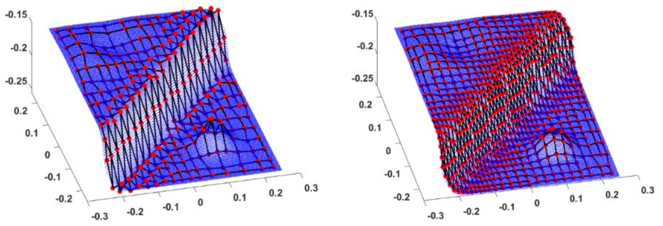
T-spline surfaces were introduced as a generalization of NURBS surfaces with T-junctions to face that challenge. These surfaces inherit the good properties of NURBS, such as partition of unity, point-wise non-negative, affine covariance and a convex hull property [18]. They are defined by a control grid called a T-mesh, which represents a group of control points connected by several straight lines. The mesh becomes dense and close to the point cloud as the number of control points increases (Figure 1, right and left, visualization using Matlab software).
The control vertices in the T-mesh (red points in Figure 1) correspond to knots in a parametric pre-image (Figure 2). The number of knots in every row and column is not necessarily the same. As shown in Figure 2 (right), the interrupted knots form the letter T, from which the term T-spline was derived. The so-called T-junctions within the T-splines framework enable a local refinement: control points can be inserted into the control grid without adding a whole row or column of control points. In this way, the number of redundant control points in T-spline surfaces is minimized compared to NURBS surfaces. A NURBS mesh is simply a rectangular grid, i.e., a T-mesh without T-junctions.
We call the parameters that define the surface domain, which is usually described as two real numbers ranging from 0 to 1. Starting from a two-dimensional T-spline pre-image, the position of a surface point on the T-spline surface is given by
where represents the control vertex, is the control points’ weights usually taken to 1 in T-spline surface fitting and is the set of T-spline blending functions. The set of blending functions is defined as the product of two univariate B-spline basis functions determined by two knot quintuples following
If we take the u direction as an example, the B-spline basis functions are recursively defined as
where corresponds to , i.e., cubic basis functions [18]. In that case, we usually define as the knot vector for NURBS, a sequence of non-decreasing parametric values of length . The knot vector for T-splines is locally defined as , and similarly for the parameter as , according to [28]. These knot quintuples are associated with each control point and are obtained from the T-mesh in the parametric domain (so-called pre-image, see Figure 2). Based on the knot quintuple, the blending functions are calculated from the recursion formula given in Equation (3). If one inserts a knot into the knot quintuples, the “old” blending function is decomposed into a linear combination of a few new blending functions that have finer knot quintuples; see [18] (Chapter 3) for a detailed example.
T-splines allow local refinement, i.e., a local definition of the knot vector and the associated control points. They are, therefore, much more flexible than B-splines. This property can be mathematically shown if we denote the rational blending function with weight 1 as . The T-spline surface can be rewritten as , or in matrix form as
with being the rational blending functions and the matrix of control points, respectively. This definition shows that there is no longer any limitation from the tensor product definition, for which we would have
Compared to Equation (5), the coefficient of each vertex (or control point in the parametric space) in Equation (4) within the T-splines framework is simply the value of a rational blending function. The latter denotes its local influence on the surface point which is expressed as a linear combination of control vertices.
2.2. Refinement Strategy
As it has been mentioned previously, given a rectangular domain, a T-mesh is a partition of the parametrized domain, i.e., a rectangular grid for which T-junctions are allowed. A T-mesh can be locally refined when individual selected cells (Figure 3 “cell to be refined in dark red”) are divided along their longest grid span. In this contribution, we make use of the refinement algorithm of [38]. This algorithm has a linear computational complexity in terms of the number of mesh elements marked and generated. It provides smooth transitions between refined and unrefined domains, preventing unwanted oscillations on the surface near the refined domains. Its principle is illustrated in Figure 3 by means of a simple example. More complex refinement examples are to be found in the dedicated publication. The surroundings of the cell (light red) to be refined are checked to search if they are coarser than the cell itself (Figure 3 “is it coarser than”). The refinement is not only performed for the cell under consideration but also involves its surroundings. A classical hierarchical approach would have halved the marked cell in the two directions, leading to four refined cells, without accounting for the neighborhood of the cell.
In order to obtain an admissible T-mesh, a few rules need to be accounted for, described in [29]. The linear independence of the T-spline blending functions, for instance, and the partition of unity have to be guaranteed so that more control points may need to be added to the T-mesh. Additionally, the sum of the T-spline blending functions should always equal one.
2.3. Iterative T-Spline Surface Approximation Using Least Squares
The goal of surface fitting is to find the best T-spline surface based on a certain criterion [18] for T-splines fitting. In this contribution, we search for a surface that minimizes the sum of the squared parametric distances between —the parametrized Cartesian observations of length —and the surface, which we solve as a standard least squares problem, i.e., , with as the L2 norm or Euclidian distance. This optimization problem can be summarized in matrix form as , where is an matrix that contains the estimation of the blending functions at the parameters’ location, i.e., its elements are , is the vector of control points and . The matrices and depend on the underlying T-mesh via the two knot vectors .
The solution is unique due to the linear independence of the blending functions. It determines the estimates of the control points that form the parametrized T-spline surface given by , where is used for “estimates.” The error term is defined point-wise as
A refinement is performed in the element regions that contain a minimum of, e.g., three observations associated with an error term higher than a given threshold , i.e., . All cells containing such data points are refined following the algorithm proposed in the previous section. The refinement is not obligatorily dyadic, i.e., in the two parametric directions: this is the main difference to a NURBS refinement. The value of three observations is the choice of the user and could be reduced or increased to avoid too fine or too coarse a refinement, respectively. Similarly, the choice of the threshold is left to the user’s convenience. A few cells are refined with a large threshold. On the contrary, all cells will be halved for a low ; this is the same as performing a global approximation with NURBS and may lead to an overfitting. In this contribution, we propose setting , with being the standard deviation of the z-component of the Cartesian observations, to prevent unnecessary refinement that would make the surface estimated closer to the noisy observations than to the true one. The refinement is stopped when either no cells need to be refined or a maximum number of iterations is reached.
The methodology used is summarized in a flowchart form in Figure 4.
2.4. Criterion to Judge the Goodness of Fit
The main indicators used to judge the goodness of fit are usually:
- The RMSE regarding the points to be approximated and also called average distance . Alternatively, an a posteriori variance factor could be computed, i.e., , as the mean of the error term computed with LS is 0. Since in this contribution , we will use the average distance RMSE, which has similarities to the average distance, as used in [26].
- The maximal error, .
- The number of points outside the tolerance , i.e., for which once the maximum of iterations allowed is reached. Note that the refinement is performed only if at least three points are outside the tolerance in this contribution. Consequently, even if the refinement stops, some cells may contain one or two points outside the tolerance. This strategy was chosen to avoid unnecessary cell refinement linked with the computational burden, when the observations may contain outliers.
We note that the RMSE is based on the scattered and noisy points to be approximated and not on the reference surface, which is unknown in a real case. It is possible that a small RMSE is linked with an unwanted fitting of the noise and is not favorable. This challenge is addressed in the next section.
3. From the 3D Printing of the Reference Surface to Its Scanning and Fitting
In this section, we will assess the goodness of fit to a known reference by printing a mathematical surface in 3D, approximated with T-splines. The methodology is summarized in a flowchart form in Figure 5. We will, firstly, briefly present how the 3D printing of a mathematical surface can be performed (steps 1, 2 and 3 in Figure 5). We will further explain the challenges solved to eliminate the noise and artefacts introduced from the 3D printer (Figure 5, steps 4 and 5), what we call “droplet modeling” (step 6 in Figure 5). This elimination is made necessary for the sake of comparison with the reference surface after the fitting. In further steps (steps 7 and 8 in Figure 5), we will explain how the surface was scanned with a TLS under various scanning configurations. Finally, the results of the T-splines approximation of the calibrated 3D body will be discussed.
3.1. Mathematical Surface
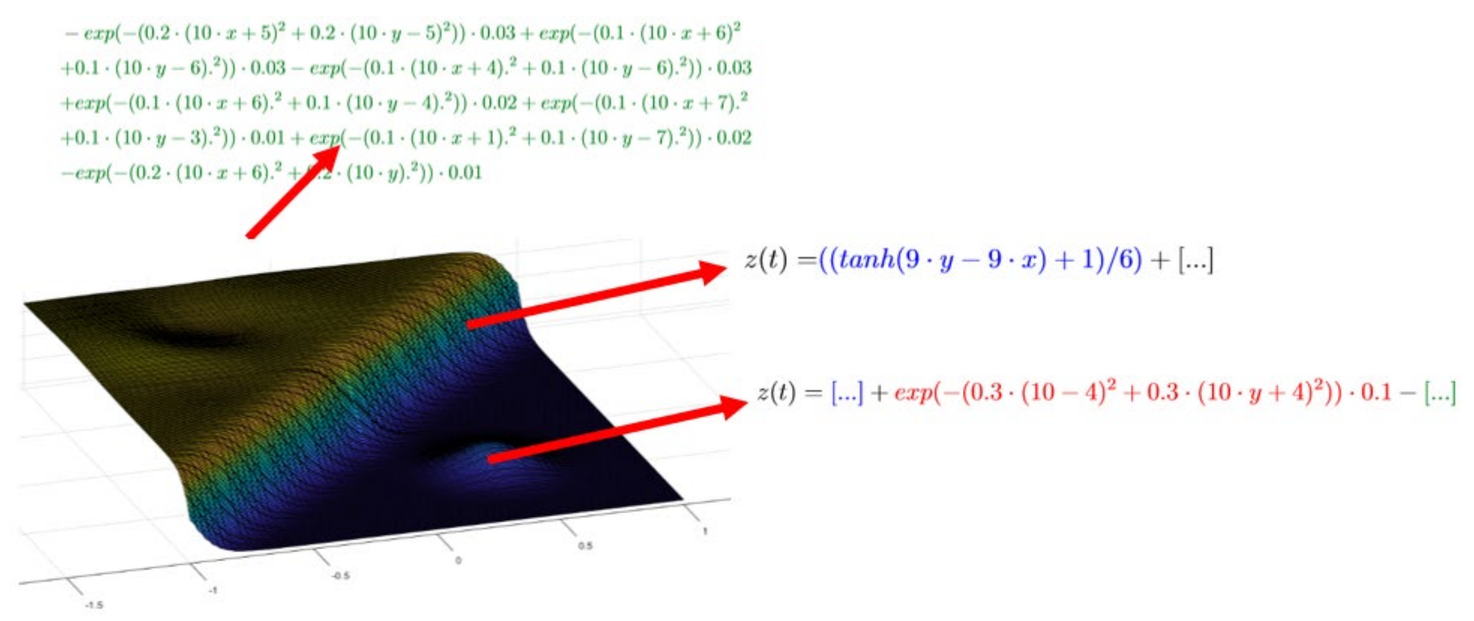
We will generate a reference T-spline surface using a 3D printer with the aim to verify the trustworthiness of a surface fitting with T-splines with respect to NURBS from TLS point clouds. The area of the chosen shape is completely defined using the following formula, whereby the range of values for x and y is between −1 and 1 for the generation of the surface.
Figure 6 shows the various components of the mathematical surface and their corresponding equations. The red part corresponds to a Gaussian bell, which could represent a mountain in real life. The blue part is a kind of dam. The waves serve to stabilize the surface to enable 3D printing and are obtained from the green part.
This surface was discretized and parameterized using the uniform method. Another parametrization strategy would be the chord length method; such investigations are beyond the scope of this paper but will not affect the generalizability of our results about the goodness of fit using T-splines. The 40,000 points generated were approximated with T-splines. We chose a threshold of 0.001 and a refinement strategy for which the cells are refined if they contain more than three points outside the tolerance. We justify this choice to avoid a level of refinement at the edges of the scanned printed surface, where a mixed pixels effect may happen [39]. We obtained an error-free approximated surface after seven iterations. The final T-mesh is shown in Figure 7 and will serve as a reference for the following investigations (step 1 in Figure 5).
3.2. 3D Printing
In this section, we shortly introduce how the mathematical surface from Figure 6 could be printed in 3D.
3.2.1. Principle
Three-dimensional printing is an additive manufacturing process in which material is joined layer by layer to create a 3D object. The starting point is a digital volume model created on the computer that describes the surface of the object to be manufactured. This model is converted into a file that is compatible with the 3D printer so that it can be processed. The STL format has established itself as the standard. In this format, the surface of the object is described by a network of triangular areas. The object described by the file generated is divided into layers. A common and widespread method is fused layer modeling, which is a cost-effective and fast variant. This method was chosen here to reduce the cost for a first investigation to test our methodology for assessing the goodness of fit with T-splines. Other larger surfaces will be printed in a higher quality using other methods in the future. Since a calibration of the object will be performed, the results of our investigations are not affected by the 3D printing method.
A prerequisite for 3D printing is the use of materials that melt or can be deformed when exposed to heat, such as thermoplastics or modeling wax. The material selected was a polyactid (PLA-HAT), which is melted by a heating element on the printhead and applied to the location desired using the movement possible in three spatial axes. The subsequent cooling hardens the material and the next layer can be applied over it.
3.2.2. Preprocessing
In a pre-step and following Section 3.1, we generated a point cloud using the equation proposed. This point cloud consists of 40,000 points, which are built up in a uniform grid of 200 × 200 points. The distance of a point to its four direct neighbors in the x and y directions corresponds to 0.005. The plane produced by 3D printing was chosen to have a size of 50 × 50 cm, limited by the specificity of the 3D printer used: we wished to print the surface as a whole corpus and not as patches to avoid junctions and increase the quality of the printing. The unit of the coordinates of the 3D model was mm. Consequently, the point cloud generated was scaled with a scale factor of 250. The resulting distance between the points and the four direct neighbors was 2.5 mm in the x and y directions.
The points were meshed with one another with the help of triangular areas to meet the requirements of a file for 3D printing. We carried out a Delaunay triangulation: three points are connected to triangles in such a way that there is no other point within a circle of three points. As a result, the individual triangular areas do not overlap and there are no gaps. Three walls were drawn down from the edge to create a volume model from the surface model. This allows the level being printed to be set up lying on all three walls or standing on one wall. The resulting volume model was then divided into layers. The 3D printing process selected (fused layer modeling) for manufacturing the object is accounted for to optimally adapt the formation of the layers. The layers were each 0.2 mm thick. The surface obtained is shown in Figure 8 (top, left).
3.3. TLS Measurements
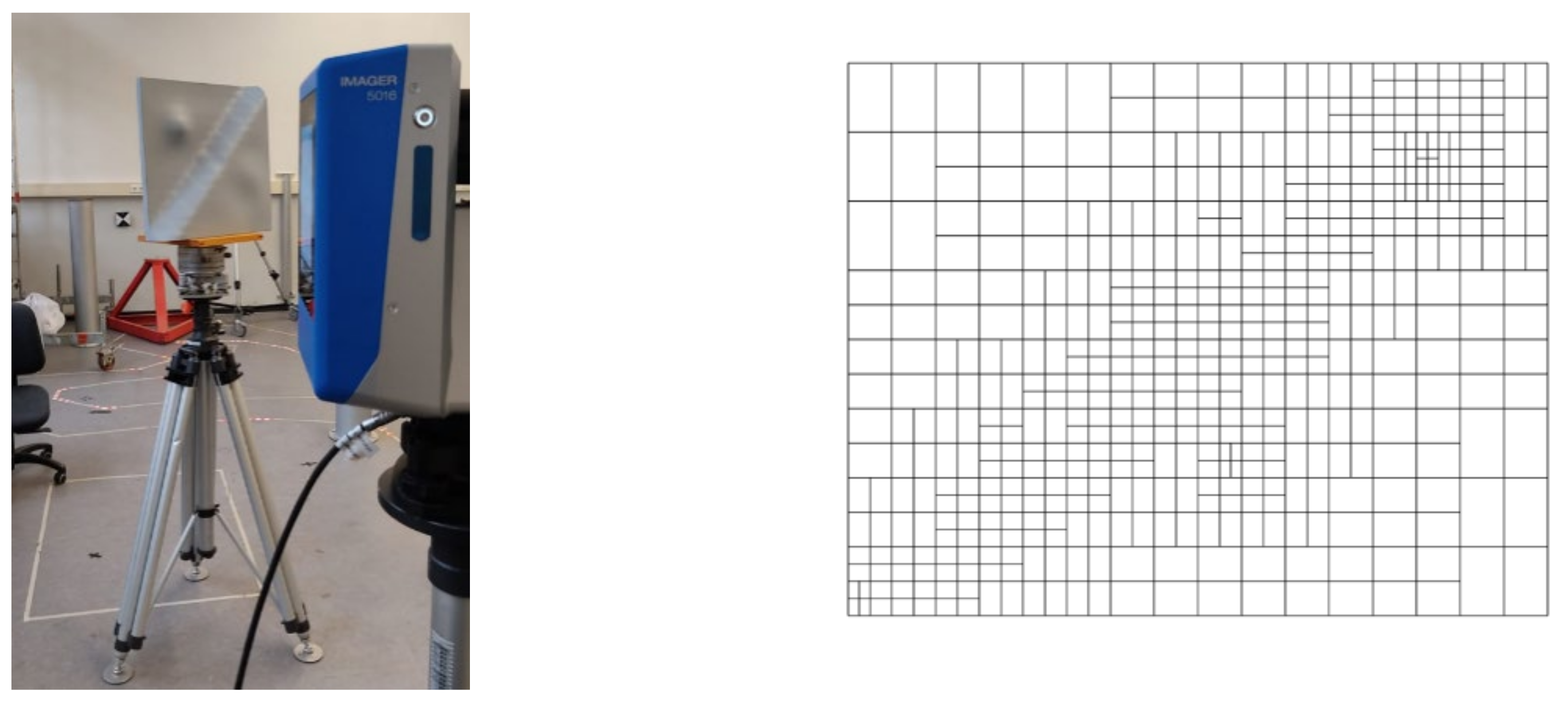
The measurements of the printed surface took place in the measuring laboratory of the Geodetic Institute in Hanover. We made use of a phase scanner, Zoller + Fröhlich Imager 5016 from Zoller & Fröhlich GmbH, Wangen, Allgäu, which is well designed for short-range indoor measurements. We varied the angles of incidence under which the printed surface was scanned from 0° to 60° and the distance from 2 to 6 m by steps of 2 m. We ensured that the angle of incidence for the reference configuration used for calibration purposes [2 m, 0°] is almost parallel to the face normal of the panel. We did not ensure a 0° tilting by using more accurate devices as we aim to model the artefacts, i.e., what we call “calibration” in this contribution. The measurements were conducted with the resolution high and quality high, i.e., a laser measuring frequency of 136 719Hz and 10,000 pixels/360°. The choice of this setting for the calibration is justified by the fact that the approximation with T-splines remains manageable on a normal computer, while, simultaneously, the level of detail is sufficient.
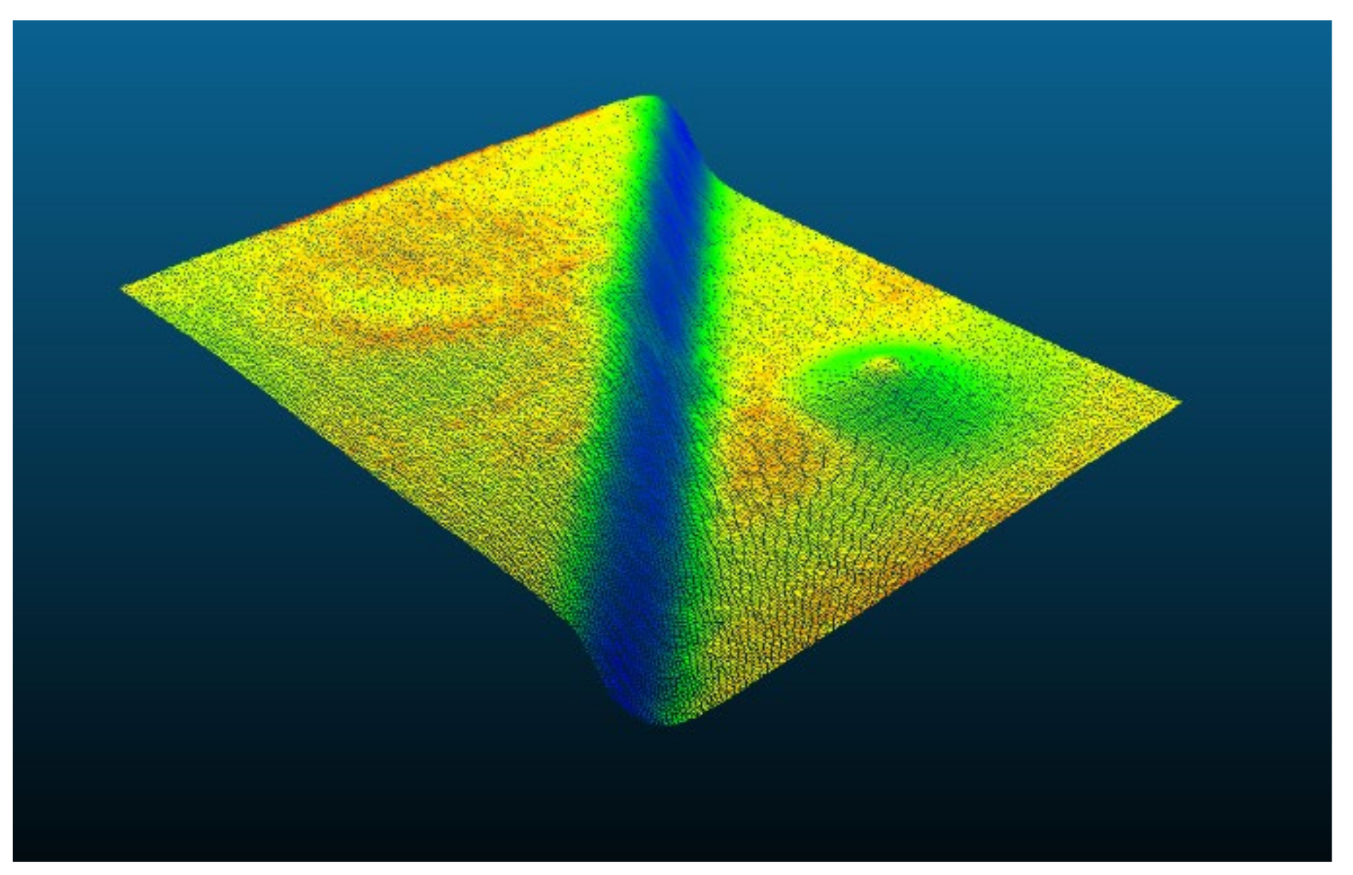
The 3D-printed planes were cut out of the whole point cloud in a preprocessing step: The free software CloudCompare was used to process the 3D point clouds (Figure 8 down). The edges of the plane were treated with care with the aim of avoiding mixed pixels [39]. After removing the other objects contained in the point cloud that do not belong to the plane, the latter was adapted to the digital reference model. In this way, the measured plane, the reference model and the T-meshes calculated from the T-splines approximation can be easily compared. We used the iterative closest point algorithm to minimize the difference between the point clouds by rotating and translating them [40].
3.4. Calibration of the Printed Surface
Unfortunately, the printed surface shown in Figure 8 (top, left) is not exactly the reference which we expected. Some artefacts coming from 3D printing arose, such as droplets, meaning that the printed surface was ground at some points. When performing the approximation with T-splines with a threshold of 1 mm, the T-mesh in Figure 8 (top, right) after eight iterations shows that the algorithm tried to approximate artefacts; this is a logical result. In this section, we follow the idea of subtracting from each point cloud or approximated point cloud these “mathematical droplets,” independently of the scanning configuration (tilt, distance), as we wish to fit the mathematical reference surface and not the reference surface with the droplets (steps 4 and 5 in Figure 5). This so-called “calibration” will allow a comparison of the mesh and the RMSE obtained with the true reference, as defined in 3.1.
To reach that goal, we performed 100 repetitions of measurements, known as “Monte Carlo” measurements. They serve to prevent undesired effects that cannot be repeated from influencing the calibration. The resulting 100 point clouds were approximated with T-splines with the threshold of 1 mm and a maximum of ten iterations. The resulting mathematical surfaces and the reference were evaluated on 250,000 equidistant parameters in both directions (500 × 500). The differences between the reference and the 100 approximations were then formed and averaged, as shown in Figure 5 (steps 4 and 5). As a result, the “mathematical droplets” remained. They are depicted in Figure 9 (left). These artefacts are a peculiarity of 3D printing: more material was used at the Gaussian bell, and a grinding was performed along the dam.
The obtained surface was finally subtracted from each approximated point cloud in order to enable a comparison with the unnoisy mathematical reference surface. The point-wise error in the z direction after calibration and re-approximation of the calibrated point cloud is shown in Figure 9 (right). It highlights the goodness of the calibration: no outliers or spurious patterns can be seen, and the null hypothesis that the point-wise error term should correspond to white noise could not be rejected with a confidence level of 5% using the Lilliefors test [41].
Table 1 summarizes the results of the approximation obtained before and after calibration using the criteria introduced in Section 2.4. The following remarks can be made:
- There is no error after the calibration compared to the 41 before calibration. This result confirms the presence of artefacts on the printed surface that were approximated by the iterative algorithm before calibration, leading to cells that still contain one or two errors.
- The Monte Carlo measurements permit the generation of a highly accurate calibrated surface: the point cloud approximated after the subtraction of the “droplets surface” became close to the printed reference; the RMSE reached 3.2 × 10⁻² mm, which corresponds to a decrease of 40% w.r.t. the RMSE before calibration. This small value after calibration highlights the high trustworthiness of the approximation, i.e., the closeness to the mathematical surface.
- The T-mesh is similar to the reference one, up to four points that were added supplementarily.
The result of the calibration indicates that T-spline surfaces permit the approximation of a noisy and scattered point cloud corresponding to a smooth surface with a high confidence regarding a known reference. The same procedure will be used in the future for surfaces with sharp edges to analyze the goodness of fit. We are highly confident that the approximation will also be of good quality; T-splines are widely used in computer graphics where such challenging geometries occur [18].
4. Approximation: Impact of the Scanning Configuration
In this section, we vary the scanning configuration (distance and tilting) and more specifically investigate the following:
- The approximation with T-splines and NURBS after calibration of the surface;
- The extent to which the original T-mesh can be reused for various configurations to avoid repeating the adaptive refinement and save computational time.
4.1. T-Splines Approximation by Varying the Scanning Configuration
The printed surface was scanned under different configurations by varying both the distance to the scanner and the tilting of the printed surface. In this section, we perform an adaptive T-spline surface approximation following the methodology presented in Section 3. The results are presented in Table 2.
4.1.1. Varying the Distance
When the distance is varied from 2 to 6 m, we notice the following:
- The RMSE for the reference surface increases by a factor between 1.2 and 1.5 approximately between the distances 4–2 and 6–4 m. This result seems strongly plausible as the number of scanned points decreases with the scanning distance. The number of points is about 140,000 for the distance of 2 m, 36,000 for 4 m and 18,000 for 6 m.
- There are no points outside tolerance except for the challenging tilting of 60° for which the number of errors reaches 25. This value is small compared with the size of the point clouds.
- The number of control points decreases slightly as the number of points to approximate becomes smaller, which is highlighted in Figure 10 with the corresponding T-meshes.
4.1.2. Varying the Tilting
Similarly, for a given distance, the tilting
- Leads to an approximative increase in the RMSE by a factor 2 between 0° and 60°. The maximum error becomes higher by up to a factor 3 for the distance of 2 m.
- Affects the repartition of the control points along the diagonal, i.e., along the dam. There are slightly less control points at the edges than for the reference T-mesh. This effect is linked with the repartition of the scanned points in space. This result has to be weighted by the very small value of the RMSE, making the differences statistically nearly insignificant.
- Does not lead to a strong variation in the number of control points to estimate. A maximum difference of 20 is observed due to the decrease in the number of scanned points, or the inclusion of lines in the T-mesh by the refinement algorithm caused by challenging geometries. Once more, the difference cannot be considered as significant and is not synonymous with a higher computational time.
- Increases the number of iterations needed to reach the tolerance. This effect is due to data gaps, shadowing effects or systematic errors, which necessitates a higher refinement level to reach the tolerance.
4.1.3. Further Comments and Conclusion
Table 2 shows that the RMSE for the reference surface stays below the millimeter level, independently of the scanning configuration. This highlights (i) the high trustworthiness of the approximation with T-splines with respect to the reference surface as well as (ii) the goodness of the calibration that was able to eliminate artefacts. The T-meshes are close to the reference for all other scanning configurations. We propose using this property in Section 4.3. to investigate the extent to which the computational time can be saved to avoid adaptive refinement in the case of rigid body motion.
The same investigations were performed for other scanning settings (super high and middle at a scanning frequency of 546,876 Hz and 136,719 Hz, respectively, for the setting normal). The results are not presented for the sake of brevity but can be made available on demand. They are similar to the results described in this contribution.
4.2. Comparison with NURBS
For the sake of completeness, we performed a comparison with NURBS (see Section 2.1) with the aim to highlight the potential of local refinement with T-splines for approximating TLS point clouds under various scanning configurations. NURBS surfaces are a particular case of T-spline surfaces for which the threshold for refinement is set extremely low so that each cell of the mesh is halved. No local refinement is possible due to the tensor product formulation: even if the errors inside a domain are below the noise level, the noise level will be refined at each following iteration. The risk is the fitting of the noise, the so-called “overfitting”. We intuitively illustrate this challenge: Figure 11 exemplarily shows what an overfitting would look like for an original smooth surface approximated from a noisy point cloud; depending on the level of iteration, the fitted surface is altered by the noise in a different way, becoming more and more scattered (Figure 11 left versus right) if too many iterations are performed. This effect is strongly unwanted as outliers/Gaussian noise can potentially be fitted.
In this contribution, we aim to perform a fair comparison between the T-splines and the NURBS surface fittings. Consecutively, we fixed the number of parameters to estimate for both strategies so that the computational time for the two approximation methods is similar. The closest number of control points compared to the T-splines fitting is 665 points for NURBS, reached after six iterations. The corresponding results for the approximation are presented in Table 2 under brackets. The lack of local refinement leads to an increase in the RMSE of the reference by up to a factor 5 as well as a higher maximum error with respect to the results using T-splines. Increasing the number of iterations would evidently decrease the RMSE. Using our Matlab implementation, seven iterations led to a slow decrease in the RMSE by a factor 1.2 linked with an increase in the computational time by a factor 3 due to the high number of basis functions to evaluate. Consecutively, it is mandatory to weight the extent to which further iterations should be performed in terms of computational time and overfitting when approximating with NURBS. Overfitting can additionally lead to an artificial and risky decrease in the RMSE. T-spline surface approximation grandly avoids this drawback due to the powerful local refinement.
4.3. Avoiding Adaptive Refinement in Case of Rigid Body Motion
The similarity of the meshes, as shown in Figure 10, raises the question of the opportunity to use the reference mesh of Figure 2 to approximate other point clouds from the same object, provided that its shape does not change strongly but only its orientation in space (distance, tilting). We call such a deformation a “rigid body motion”. The proposed strategy
- Would be validated if the RMSE or the number of points outside tolerance does not change drastically between the reference and the T-mesh as used in Section 4.1 (Figure 10) to approximate the point clouds.
- Would avoid the re-computation of the basis functions and save computational time drastically when the same object is scanned at different epochs but only its orientation in space changes: no adaptive refinement would have to be performed for the second point cloud, and the approximation could be directly computed.
- Makes use of the property of a T-mesh: the T-mesh acts as a filter so that additional effects (systematic or stochastic information arising, e.g., when varying the tilting) could be eliminated.
The corresponding results for the approximation of the point clouds using the reference T-mesh are given in Table 3. The RMSE for the reference remains below the millimeter level and increases slightly as the number of errors increases, i.e., mainly for the angle of 60°, exemplarily from 2 × 10⁻² to 4 × 10⁻¹ mm for [2 m, 0°] to [2 m, 60°]. As it has been mentioned previously, the reference T-mesh we used acts as a filter of “rest effects” that were not modeled after the calibration, which results in a slightly lower RMSE regarding Table 2 for some configurations.
Similar to Table 2, Table 3 highlights the goodness of fit of the approximation with T-splines from a noisy and scattered point cloud, even if an approximated T-mesh is used. The number of points outside the tolerance stays under 1% of the total number of scanned points. The RMSE stays constant independent of the tilting or distance used for the scanning, i.e., no sharp increase is noticed. As previously mentioned, the impact of shadowing, data gaps or outliers can be reduced due to the approximated T-mesh. The approximated T-mesh may be coarser with regard to the original one used in Table 2.
4.4. Concluding Remarks
The following conclusions are drawn from the previous investigations:
- We can be highly confident about the goodness of fit of a T-spline surface to a point cloud from a smooth surface.
- When the point clouds are rigidly deformed, an approximated mesh can be used with high confidence and a low impact on the RMSE for the reference, as only 1% of the points were outside the tolerance.
- Compared with the global refinement performed with NURBS, the main advantage of the local refinement strategy is to approximate the point cloud with a high definition only in some specific domains. Global refinement with NURBS may lead to an overfitting as the number of iterations increases. It is further linked with a strong increase in the computational time as the number of parameters to estimate increases. Local and adaptive refinement strategies should be preferred in the case of noisy and scattered point clouds.
5. Application: A Bridge under Load
In this section, we apply the results of the analysis from the 3D-printed surface. Accordingly, we will fit two epochs of TLS observations with T-splines. Due to the assumed rigid body motion between the epochs, we will make use of the strategy developed in 3.5. to simplify the iterative refinement and save computational time.
5.1. Short Description of the Dataset
In this section, we use a real dataset of a historic masonry arch bridge over the river Aller near Verden in Germany to judge the extent to which T-splines are appropriate to approximate a dataset from TLS. The TLS observations stem from an experiment carried out within the framework of the interdisciplinary project “Application of life cycle concepts to civil engineering structures” [42]. Loads of increasing weights were artificially added onto specific parts of the bridge to simulate the impact induced, e.g., by car traffic. The deformation is, thus, expected to have happened in the vertical direction and have the strongest magnitude for the last point clouds named E55. The profiles were captured using a Z + F Imager 5006H at a sampling rate of 500,000 points per second.
Using a specific software (CloudCompare), a small patch was selected on the point clouds E00 and E55 (reference and fifth load step, respectively). It is depicted in Figure 12. We aim to
- approximate the two patches with T-splines;
- compare the T-meshes;
- perform the approximation for epoch E55 on the same T-mesh as epoch E00, i.e., without iteration. This will allow us to judge the feasibility of our methodology in the case of rigid body motion.
We parametrized the point clouds using the uniform method, justified by the relatively smooth and uncomplicated geometry of the point clouds selected [27]. We note that with real data, the reference surface, i.e., the “truth”, is unknown.
5.2. Results of the T-Splines Approximation and Comparison with NURBS
The approximation with T-splines was performed intentionally with a coarse threshold of 1 mm with the aim not to approximate the noise. Its standard deviation was estimated at 0.5 mm for the range, following the manufacturer’s datasheet. The threshold was chosen slightly over the estimated value for the standard deviation of the Cartesian coordinates. This way, adaptive refinement is performed only in the domain when necessary. This threshold is high enough to avoid a uniform and global refinement corresponding to a NURBS fitting: (i) computational time is saved, and (ii) overfitting is reduced. A maximum of ten iterations was fixed. The algorithm converges after eight iterations for both patches. The T-spline surface is depicted in Figure 13 (left), for E00 and the corresponding residuals in Figure 13 (right). The results of the approximations are summarized in Table 4. We highlight that for the T-spline surface fitting:
- The residuals do not show a spurious pattern, are nearly white and are below the millimeter level in norm. We note further that the number of errors is small regarding the size of the point clouds (170,000 points). Both remarks confirm the goodness of the approximation for the threshold chosen.
- The number of control points and errors was similar for both surfaces, which has to be linked with the fact that the patch did not change in shape but only in orientation.
- The maximum error may seem large: it fortunately concerns only a few points as the small RMSE of 1 mm indicates.
Compared with NURBS, the T-splines approximation has strong advantages:
- The RMSE is similar to that for the NURBS approximation. The difference is approximately 0.1 mm for E00 (similar for E55 but not shown for the sake of shortness) and cannot be considered as significant. We insist that an RMSE that is too small is not synonymous with a good approximation, as the noise may have been fitted, as illustrated in the previous section. A good balance has to be found, by avoiding oscillations in the residuals. The residuals can be visually detected by inspecting the fitted surface.
- The number of control points to estimate for NURBS is three times higher than for T-splines for the same RMSE. This drawback increases the computational time by a factor 6 from 45 to 300 s. The corresponding NURBS mesh is shown in Figure 14 (bottom). Compared with the T-meshes of the two epochs (Figure 14, top), a lot more control points need to be introduced: 3550 versus 1141.
- The number of errors for NURBS increases with respect to the T-spline approximation due to the global refinement since all the cells of the mesh are halved, which corresponds to an extremely small threshold in an adaptive scheme.
This short example should convince the readers of the flexibility and computational advantage of a T-spline over a NURBS surface.
5.3. “Re” Using the T-Mesh for Deformation Analysis
Following the investigations of Section 4.3, we computed the patch of the second epoch E55 with the mesh of the first epoch E00. Since the patch of E55 is not expected to have strongly varied in shape with the load but only in orientation, this strategy is optimal to save computational time for the fitting of the second epoch: a re-computation of the basis function is avoided. We found that the computational time saved was 31 s, compared to the 45 s needed for the first epoch. This time may seem high; we should mention that our algorithm is not fully optimized yet and implemented in Matlab. The RMSE was slightly higher (9.9 × 10⁻¹ versus 9.1 × 10⁻¹). We link this discrepancy with the fact that the point clouds were not recorded at the same time for the load of E55 as for E00. We mention that the difference stays below the millimeter level.
The Hausdorff distance between the two surfaces was not affected by reusing the T-mesh [27]: we found a value of 8.9 mm using the original accurate T-meshes versus 9.0 mm for the simplification. The difference below the millimeter level cannot be considered as statistically significant and has to be weighed against the computational time saved.
5.4. Summary
This real case study of a bridge under load confirmed the potential of a local refinement strategy for fitting point clouds from TLS observations. The advantages were already highlighted in Section 3 by means of a 3D-printed reference surface. With the adaptive refinement method, we were able to
- Reduce the computational time regarding a global surface fitting using NURBS. The adaptive local refinement strongly decreases the number of parameters to estimate for the same order of the RMSE.
- Simplify the computation of the control points of the second epoch by using the same mesh as for the first epoch. This was made possible since the deformation of the patch was rigid, i.e., only its orientation changed and its shape was not strongly affected by the load.
- Show that the distance between the two point clouds was not affected by the simplification, which is an important property for further deformation analysis.
6. Conclusions
The potential of TLS-based deformation analysis is high due to the fast and simple data acquisition, the high point density and the possibility of scanning whole areas of interest. Unfortunately, the processing of point clouds with millions of observations may be computationally demanding. Surface fitting with splines provides an alternative by storing the observations in a compact form with only a few parameters to be estimated. At the same time, rigorous test statistics are possible, which can include stochastic information about the observations. Without using any gridding of the observations, local refinement strategies to fit the scattered and noisy point clouds are a promising alternative to the widely used NURBS in geodesy. In this contribution, we have shown that T-spline—a generalization of NURBS using a T-junction in a mesh—is a promising approach: an adaptive local refinement is carried out only at the problematic regions. The latter can be stopped based on a threshold or after a given number of iterations. The algorithm enables one to output a more compact surface with fewer control points to be estimated than with NURBS. In this contribution, we have highlighted that the computational time saved is far from negligible. Furthermore, we assessed the goodness of fit by using a reference 3D-printed surface (i) scanned with a TLS under various scanning configurations and (ii) calibrated to eliminate the artefacts of 3D printing. We demonstrated that a reference mesh can be used in the case of rigid body motion for two epochs of observations without affecting the approximation. We applied these results successfully to a real data analysis corresponding to a bridge under load.
Our results pave the way for new applications of local refinement strategies, from surface fitting to registration or deformation analysis. The approach of finding the control points is global, i.e., it has to be updated at each iteration by the LS method. Correspondingly, the T-spline surface is optimal in the L2 norm for a given T-mesh topology, but the iterative fitting remains time-consuming. In the next study, we will implement other methodologies based on local least squares and assess how point clouds with edges or more challenging geometries can be fitted optimally with T-spline surfaces.
Author Contributions
G.K.: conceptualization, methodology, investigation, analysis and writing; N.S. and J.H.: investigation and review. All authors have read and agreed to the published version of the manuscript.
Funding
This study is supported by the Deutsche Forschungsgemeinschaft under the project KE2453/2-1. The authors warmly thank Morgenstern for interesting discussions. The publication of this article was funded by the Open Access Fund of Leibniz Universität Hannover.
Institutional Review Board Statement
Not applicable.
Informed Consent Statement
Not applicable.
Data Availability Statement
Data available on demand.
Conflicts of Interest
The authors declare no conflict of interest.
References
- Vosselman, G.; Maas, H.-G. (Eds.) Airborne and Terrestrial Laser Scanning; Whittles: Dunbeath, UK, 2010. [Google Scholar]
- Hohenthal, J.; Alho, P.; Hyyppa, J.; Hyyppa, H. Laser scanning applications in fluvial studies. Prog. Phys. Geogr. 2011, 35, 782–809. [Google Scholar] [CrossRef]
- Pu, S.; Vosselman, G. Knowledge based reconstruction of building models from terrestrial laser scanning data. ISPRS J. Photogramm. Remote Sens. 2009, 64, 575–584. [Google Scholar] [CrossRef]
- Watt, P.J.; Donoghue, D.N.M. Measuring forest structure with terrestrial laser scanning. Int. J. Remote Sens. 2005, 26, 1437–1446. [Google Scholar] [CrossRef]
- Liang, X.; Kankare, V.; Hyyppä, J.; Wang, Y.; Kukko, A.; Haggrén, H.; Yu, X.; Kaartinen, H.; Jaakkola, A.; Guan, F.; et al. Terrestrial laser scanning in forest inventories. ISPRS J. Photogramm. Remote Sens. 2016, 115, 63–77. [Google Scholar] [CrossRef]
- Lindenbergh, R.; Uchanski, L.; Bucksch, A.; van Gosliga, R. Structural monitoring of tunnels using terrestrial laser scanning. Rep. Geod. 2009, 87, 231–238. [Google Scholar]
- Heritage, G.L.; Large, A.R.G. Laser Scanning for the Environmental Sciences; Wiley-Blackwell: New York, NY, USA, 2009. [Google Scholar]
- Teza, G.; Galgaro, A.; Zaltron, N.; Genevois, R. Terrestrial laser scanner to detect landslide displacement fields: A new approach. Int. J. Remote Sens. 2007, 28, 3425–3446. [Google Scholar] [CrossRef]
- Monserrat, O.; Crosetto, M. Deformation measurement using terrestrial laser scanning data and least squares 3D surface matching. ISPR J. Photogramm. Remote Sens. 2008, 63, 142–154. [Google Scholar] [CrossRef]
- Lague, D.; Brodu, N.; Leroux, J. Accurate 3D comparison of complex topography with terrestrial laser scanner: Application to the Rangitikei canyon (N-Z). ISPRS J. Photogramm. Remote Sens. 2013, 82, 10–26. [Google Scholar] [CrossRef] [Green Version]
- Lichti, D.; Gordon, S.; Tipdecho, T. Error models and propagation in directly georeferenced terrestrial laser scanner networks. J. Surv. Eng. 2005, 135–142. [Google Scholar] [CrossRef]
- Schuhmacher, S.; Boehm, J. Georeferencing of terrestrial laser scanner data for applications in architectural modelling. In Proceedings of the ISPRS Working Group V/4Workshop 3DARCH 2005: Virtual Reconstruction and Visualization of Complex Architectures, Mestre-Venice, Italy, 22–24 August 2005. [Google Scholar]
- Barbarella, M.; Fiani, M.; Lugli, A. Landslide monitoring using multitemporal terrestrial laser scanning for ground displacement analysis. Geomat. Nat. Haz. Risk. 2015, 6, 398–418. [Google Scholar] [CrossRef]
- Dierckx, P. Curve and Surface Fitting with Splines; Report Monographs on Numerical Analysis; Clarendon Press: Oxford, UK; New York, NY, USA; Tokyo, Japan, 1993. [Google Scholar]
- Holst, C.; Schmitz, B.; Kuhlmann, H. TLS-Basierte Deformationsanalyse unter Nutzung von Standardsoftware. DVW e.V.: Terrestrisches Laserscanning 2016; DVW Schriftreihe, 85/2106; Wißner: Augsburg, Germany, 2016; pp. 39–58. [Google Scholar]
- Zhang, Y.; Neumann, I. Utility theory as a method to minimize the risk in deformation analysis decisions. J. Appl. Geod. 2014, 8, 283–294. [Google Scholar] [CrossRef] [Green Version]
- Bartels, R.H.; Beatty, J.C.; Barsky, B.A. An Introduction to Splines for Use in Computer Graphics & Geometric Modeling; Morgan Kaufmann Publishers Inc.: San Francisco, CA, USA, 1987. [Google Scholar]
- Wang, Y. Free-Form Surface Representation and Approximation Using T-Splines; Nanyang Technological University: Singapore, 2009. [Google Scholar] [CrossRef] [Green Version]
- Piegl, L.; Tiller, W. The Nurbs Book. In Monographs in Visual Communication, 2nd ed.; Springer: Berlin/Heidelberg, Germany, 1997. [Google Scholar]
- Forsey, D.R.; Bartels, R.H. Surface fitting with hierarchical splines. ACM Trans. Graph. 1995, 14, 134–161. [Google Scholar] [CrossRef]
- Giannelli, C.; Jüttler, B.; Speleers, H. THB-splines: The truncated basis for hierarchical splines. Comput. Aided Geom. Des. 2012, 29, 485–498. [Google Scholar] [CrossRef] [Green Version]
- Bressan, A. Some properties of LR-splines. Comput. Aided Geom. Des. 2013, 30, 778–794. [Google Scholar] [CrossRef]
- Dokken, T.; Pettersen, K.F.; Lyche, T. Polynomial splines over locally refined box-partitions. Comput. Aided Geom. Des. 2013, 30, 331–356. [Google Scholar] [CrossRef]
- Kiss, G.; Giannelli, C.; Zore, U.; Jüttler, B.; Großmann, D.; Barner, J. Adaptive CAD model (re-)construction with THB-splines. Graph. Model. 2014, 76, 273–288. [Google Scholar] [CrossRef]
- Jüttler, B. Surface fitting using convex tensor-product splines. J. Comput. Appl. Math. 1997, 84, 23–44. [Google Scholar] [CrossRef] [Green Version]
- Skytt, V.; Barrowclough, O.; Dokken, T. Locally refined spline surfaces for representation of terrain data. Comput. Graph. 2015, 49, 48–58. [Google Scholar] [CrossRef]
- Kermarrec, G.; Kargoll, B.; Alkhatib, H. On the impact of correlations on the congruence test: A bootstrap approach. Acta Geod. Geophys. 2020, 55, 495–513. [Google Scholar]
- Sederberg, T.W.; Zheng, J.; Bakenov, A.; NASRI, A.H. T-splines and t-nurccs. ACM Trans. Graph. 2003, 22, 477–484. [Google Scholar] [CrossRef]
- Sederberg, T.W.; Cardon, D.L.; Finnigan, T.; North, N.S.; Zheng, J.; Lyche, T. T-spline simplification and local refinement. ACM Trans. Graph. 2004, 23, 276–283. [Google Scholar] [CrossRef] [Green Version]
- Zheng, J.; Wang, Y.; Seah, H.S. Adaptive T-spline Surface Fitting to Z-Map Models. In Proceedings of the 3rd International Conference on Computer Graphics and Interactive Techniques in Australasia and South East Asia (GRAPHITE ‘05), Dunedin, New Zealand, 29 November–2 December 2005; Association for Computing Machinery: New York, NY, USA, 2005; pp. 405–411. [Google Scholar]
- Skytt, V.; Harpham, Q.; Dokken, T.; Dahl, H.E.I. Deconfliction and surface generation from bathymetry data using LR B-splines. In Scattered Data Interpolation with Multilevel B-Splines; Mathematical Methods for Curves and Surfaces. MMCS 2016; Floater, M., Lyche, T., Mazure, M.L., Mørken, K., Schumaker, L., Eds.; Springer: Cham, Switzerlan, 2016; Volume 10521. [Google Scholar] [CrossRef] [Green Version]
- Lee, S.; Wolberg, G.; Shin, S.Y. Scattered data interpolation with multilevel B-splines. IEEE Trans. Visual. Comput. Graph. 1997, 3, 229–244. [Google Scholar] [CrossRef] [Green Version]
- Yang, X.; Zheng, J. Approximate spline surface skinning. Comput. Aided Des. 2012, 44, 1269–1276. [Google Scholar] [CrossRef]
- Bracco, C.; Giannelli, C.; Großmann, D.; Sestini, A. Adaptive fitting with THB-splines: Error analysis and industrial applications. Comput. Aided Geom. Des. 2018, 62, 239–252. [Google Scholar] [CrossRef]
- Morgenstern, P.; Peterseim, D. Analysis-suitable adaptive T-mesh refinement with linear complexity. Comput. Aided Geom. Des. 2015, 34, 50–66. [Google Scholar] [CrossRef] [Green Version]
- Bureick, J.; Alkhatib, H.; Neumann, I. Robust spatial approximation of laser scanner point clouds by means of free-form curve approaches in deformation analysis. J. Appl. Geod. 2016, 10, 27–35. [Google Scholar] [CrossRef]
- Koch, K.R. Fitting free-form surfaces to laserscan data by nurbs. Allgemeine Vermessungs-Nachrichten 2009, 116, 134–140. [Google Scholar]
- Hennig, P.; Kästner, M.; Morgenstern, P.; Peterseim, D. Adaptive mesh refinement strategies in isogeometric analysis—A computational comparison. Comput. Methods Appl. Mech. Eng. 2017, 316, 424–448. [Google Scholar] [CrossRef] [Green Version]
- Chaudhry, S.; Salido-Monzú, D.; Wieser, A. A modeling approach for predicting the resolution capability in terrestrial laser scanning. Remote Sens. 2021, 13, 615. [Google Scholar] [CrossRef]
- Zhang, Z. Iterative point matching for registration of free-form curves and surfaces. Int. J. Comput. Vision 1994, 13, 119–152. [Google Scholar] [CrossRef]
- Lilliefors, H.W. On the Kolmogorov-Smirnov test for normality with mean and variance unknown. J. Am. Stat. Assoc. 1967, 62, 399–402. [Google Scholar] [CrossRef]
- Schacht, G.; Piehler, J.; Marx, S.; Müller, J.Z.A. Belastungsversuche an einer historischen Eisenbahn-Gewölbebrücke. Bautechnik 2017, 94, 125–130. [Google Scholar] [CrossRef]
Figure 1.
Illustration of the control T-mesh over a given parametrized surface. Red points are the control points, black the mesh lines.
Figure 1.
Illustration of the control T-mesh over a given parametrized surface. Red points are the control points, black the mesh lines.

Figure 2.
Illustration of the concept of blending functions and control points refinement. Left: Control point P with its associated knot quintuples in both directions. Refinement and new control points P1 (middle) and P2 (right) and their associated knot quintuples.
Figure 2.
Illustration of the concept of blending functions and control points refinement. Left: Control point P with its associated knot quintuples in both directions. Refinement and new control points P1 (middle) and P2 (right) and their associated knot quintuples.

Figure 3.
Example of refinement: The patch marked (pink) contains elements that are coarser than the cell to be refined (red). The algorithm checks their patches for even coarser elements and stops after two iterations.
Figure 3.
Example of refinement: The patch marked (pink) contains elements that are coarser than the cell to be refined (red). The algorithm checks their patches for even coarser elements and stops after two iterations.

Figure 4.
Methodology of the iterative refinement with T-splines.

Figure 5.
Methodology for the calibration of the 3D-printed surface scanned with TLS under various scanning configurations.
Figure 5.
Methodology for the calibration of the 3D-printed surface scanned with TLS under various scanning configurations.

Figure 6.
Mathematical surface serving as a reference for the 3D printing after the T-spline surface approximation.
Figure 6.
Mathematical surface serving as a reference for the 3D printing after the T-spline surface approximation.

Figure 7.
T-mesh of the reference surface.

Figure 8.
Top: left: the printed surface scanned at the laboratory of the Geodetic Institute in Hanover; right: the corresponding T-mesh. Bottom: the 3D point cloud visualized using the free software Cloudcompare.
Figure 8.
Top: left: the printed surface scanned at the laboratory of the Geodetic Institute in Hanover; right: the corresponding T-mesh. Bottom: the 3D point cloud visualized using the free software Cloudcompare.


Figure 9.
Left: artefacts coming from 3D printing; right: the point-wise error after calibration.

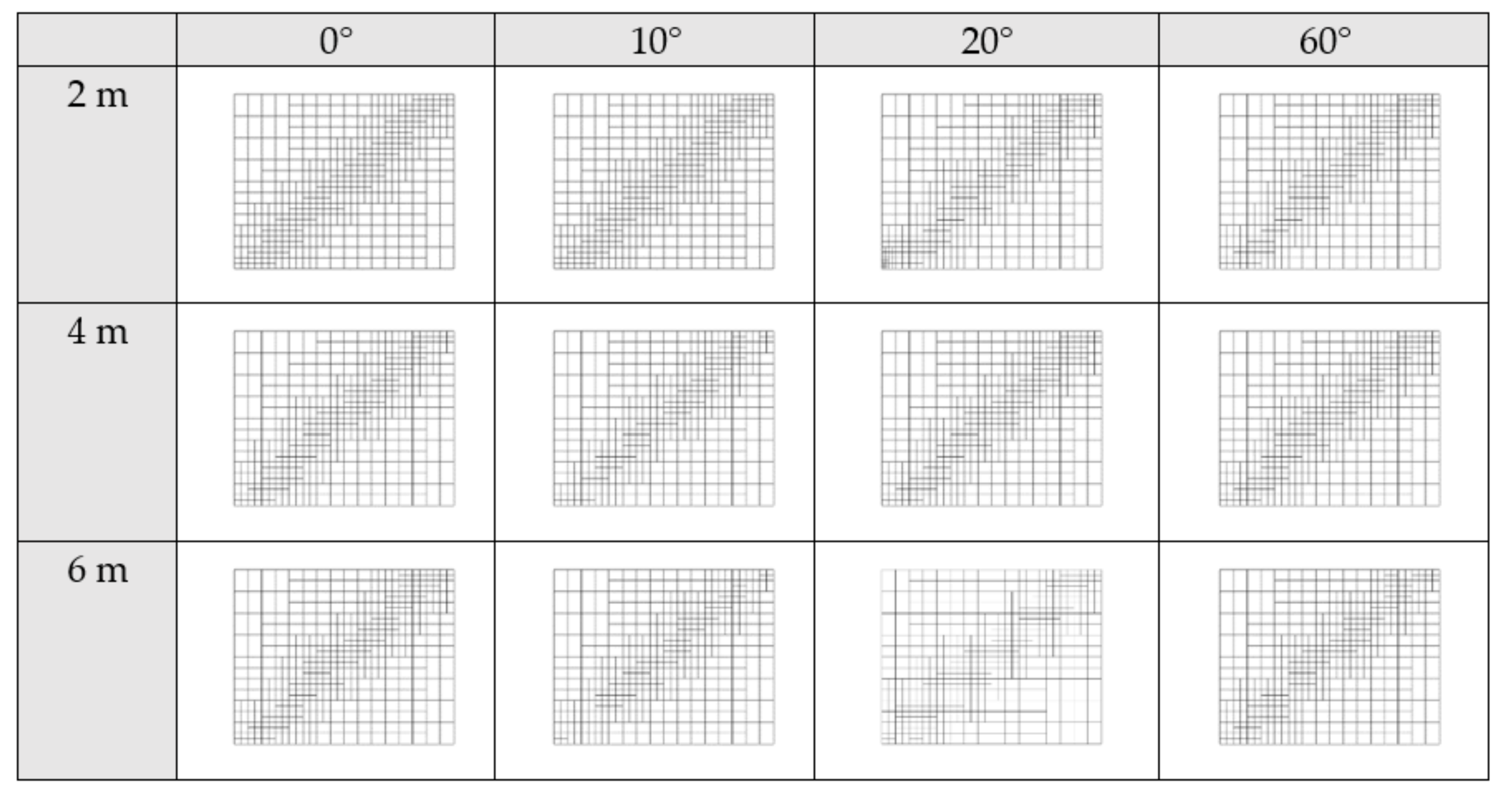
Figure 10.
T-meshes corresponding to the different scanning configurations, as presented in Table 2. Both the scanning distance angles were varied.
Figure 10.
T-meshes corresponding to the different scanning configurations, as presented in Table 2. Both the scanning distance angles were varied.

Figure 11.
Two examples of overfitting -fitting of the noise of the point cloud- in the approximation for an arbitrary smoothed surface in the parametric domain. Right: after 10 iterations; left: after 6 iterations.
Figure 11.
Two examples of overfitting -fitting of the noise of the point cloud- in the approximation for an arbitrary smoothed surface in the parametric domain. Right: after 10 iterations; left: after 6 iterations.

Figure 12.
Top: visualization of the bridge for E00 using the software CloudCompare and localization of the patches of interest (bottom).
Figure 12.
Top: visualization of the bridge for E00 using the software CloudCompare and localization of the patches of interest (bottom).

Figure 13.
Left: T-spline surface E00 in (m) with reduced z-component (m); right: residuals of the approximation in (m).
Figure 13.
Left: T-spline surface E00 in (m) with reduced z-component (m); right: residuals of the approximation in (m).

Figure 14.
Top: T-mesh corresponding to E00 (link) and E55 (right). Bottom: the NURBS mesh for E00.


Table 1.
Results of the approximation of the printed reference. The results of the approximation of the scanned printed surface before and after the calibration.
Table 1.
Results of the approximation of the printed reference. The results of the approximation of the scanned printed surface before and after the calibration.
| RMSE/Reference (mm) | Max Error (mm)/Nb of Errors | Nb of Control Points/Iterations | |
|---|---|---|---|
| Before calibration | 1.6 | 1.2/41 | 709/8 |
| After calibration | 3.2 × 10⁻² | 9.0 × 10⁻¹/0 | 593/7 |
| Printed reference to the mathematical reference | 8.1 × 10⁻² | 7.1 × 10⁻¹/0 | 597/7 |
Table 2.
Results of the approximation after calibration for different scanning configurations. The same criteria as in Table 1 are chosen to judge the goodness of fit. In brackets are the values obtained from the NURBS approximation.
Table 2.
Results of the approximation after calibration for different scanning configurations. The same criteria as in Table 1 are chosen to judge the goodness of fit. In brackets are the values obtained from the NURBS approximation.
| RMSE/Reference (mm) (NURBS) | Max Error/Nb of Errors (Max Error NURBS) | Nb of Control Points/Iterations (NURBS) | |
|---|---|---|---|
| 2 m 0° | 3.2 × 10⁻²(2.7 × 10⁻¹) | 9.0 × 10⁻¹/0 (3.3) | 593/7 (665/6) |
| 2 m 10° | 4.4 × 10⁻² (2.5 × 10⁻¹) | 6.3 × 10⁻¹/0 (3.5) | 589/7 (665/6) |
| 2 m 20° | 5.5 × 10⁻² (2.7 × 10⁻¹) | 9.7 × 10⁻¹/0 (8.6) | 611/10 (665/6) |
| 2 m 60° | 7.8 × 10⁻² (5.4 × 10⁻¹) | 2.8/21 (11) | 622/10 (665/6) |
| 4 m 0° | 5.0 × 10⁻² (2.6 × 10⁻¹) | 8.9 × 10⁻¹/0 (3.1) | 581/7 (665/6) |
| 4 m 10° | 6.7 × 10⁻² (2.5 × 10⁻¹) | 9.3 × 10⁻¹/0 (3.3) | 580/7 (665/6) |
| 4 m 20° | 7.2 × 10⁻² (2.6 × 10⁻¹) | 7.7 × 10⁻¹/0 (9.5) | 562/8 (665/6) |
| 4 m 60° | 1.0 × 10⁻¹ (7.5 × 10⁻¹) | 1.3/13 (34) | 573/10 (665/6) |
| 6 m 0° | 6.5 × 10⁻² (2.6 × 10⁻¹) | 9.1 × 10⁻¹/0 (3.3) | 563/8 (665/6) |
| 6 m 10° | 9.5 × 10⁻² (2.4 × 10⁻¹) | 9.8 × 10⁻¹/0 (3.2) | 536/7 (665/6) |
| 6 m 20° | 8.8 × 10⁻² (3.4 × 10⁻¹) | 1.1/0 (3.2) | 479/7 (665/6) |
| 6 m 60° | 1.1 × 10⁻¹ (5.2 × 10⁻¹) | 1.7/25 (3.7) | 541/8 (665/6) |
Table 3.
Results of the approximation after calibration for different scanning configurations using the reference T-mesh. The same criteria as in Table 1 are chosen to judge the goodness of fit.
Table 3.
Results of the approximation after calibration for different scanning configurations using the reference T-mesh. The same criteria as in Table 1 are chosen to judge the goodness of fit.
| Distance, Angle | RMSE for Reference (mm) | Max Error (mm)/Nb of Errors |
|---|---|---|
| 2 m 0° | 2.8 × 10⁻² | 9.0 × 10⁻¹/0 |
| 2 m 10° | 2.9 × 10⁻² | 7.0 × 10⁻¹/0 |
| 2 m 20° | 4.6 × 10⁻² | 7.5 × 10⁻¹/22 |
| 2 m 60° | 4.0 × 10⁻¹ | 1.0/335 |
| 4 m 0° | 4.0 × 10⁻² | 8.0 × 10⁻¹/0 |
| 4 m 10° | 4.8 × 10⁻² | 1.1/0 |
| 4 m 20° | 3.8 × 10⁻² | 9.5 × 10⁻¹/35 |
| 4 m 60° | 7.4 × 10⁻¹ | 1.1/287 |
| 6 m 0° | 2.8 × 10⁻² | 9.1 × 10⁻¹/0 |
| 6 m 10° | 6.1 × 10⁻² | 7.7 × 10⁻¹/0 |
| 6 m 20° | 9.2 × 10⁻² | 7.1 × 10⁻¹/25 |
| 6 m 60° | 7.5 × 10⁻¹ | 1.0/59 |
Table 4.
Results of the approximation for E00 and E55. The same criteria as in Table 1 are chosen to judge the goodness of fit. Threshold: 0.5 mm; number of iterations: nine.
Table 4.
Results of the approximation for E00 and E55. The same criteria as in Table 1 are chosen to judge the goodness of fit. Threshold: 0.5 mm; number of iterations: nine.
| RMSE for Reference (mm) | Max Error (mm)/Nb of Errors | Nb of Control Points/Computational Time (s) | |
|---|---|---|---|
| E00 | 9.0 × 10⁻¹ | 3.8/8 | 1141/45 |
| E00 with NURBS | 7.8 × 10⁻¹ | 3.6/56 | 3550/305 |
| E55 | 9.1 × 10⁻¹ | 4.0/12 | 898/43 |
| E55 with T-mesh from E00 | 9.9 × 10⁻¹ | 5/65 | 1141/10 |
Publisher’s Note: MDPI stays neutral with regard to jurisdictional claims in published maps and institutional affiliations. |
© 2021 by the authors. Licensee MDPI, Basel, Switzerland. This article is an open access article distributed under the terms and conditions of the Creative Commons Attribution (CC BY) license (https://creativecommons.org/licenses/by/4.0/).
Share and Cite
MDPI and ACS Style
Kermarrec, G.; Schild, N.; Hartmann, J. Fitting Terrestrial Laser Scanner Point Clouds with T-Splines: Local Refinement Strategy for Rigid Body Motion. Remote Sens. 2021, 13, 2494. https://0-doi-org.brum.beds.ac.uk/10.3390/rs13132494
AMA Style
Kermarrec G, Schild N, Hartmann J. Fitting Terrestrial Laser Scanner Point Clouds with T-Splines: Local Refinement Strategy for Rigid Body Motion. Remote Sensing. 2021; 13(13):2494. https://0-doi-org.brum.beds.ac.uk/10.3390/rs13132494
Chicago/Turabian StyleKermarrec, Gaël, Niklas Schild, and Jan Hartmann. 2021. "Fitting Terrestrial Laser Scanner Point Clouds with T-Splines: Local Refinement Strategy for Rigid Body Motion" Remote Sensing 13, no. 13: 2494. https://0-doi-org.brum.beds.ac.uk/10.3390/rs13132494
Note that from the first issue of 2016, this journal uses article numbers instead of page numbers. See further details here.