
Remote Sensing Image Scene Classification via Label Augmentation and Intra-Class Constraint


1
Harbin Institute of Technology, School of Electronics and Information Engineering, Harbin 150001, China
2
Helmholtz-Zentrum Dresden-Rossendorf, Machine Learning Group, Helmholtz Institute Freiberg for Resource Technology, Chemnitzer Straße 40, 09599 Freiberg, Germany
3
Institute of Advanced Research in Artificial Intelligence (IARAI), Landstraßer Hauptstraße 5, 1030 Vienna, Austria
*
Author to whom correspondence should be addressed.
Remote Sens. 2021, 13(13), 2566; https://0-doi-org.brum.beds.ac.uk/10.3390/rs13132566
Submission received: 10 May 2021
/
Revised: 18 June 2021
/
Accepted: 28 June 2021
/
Published: 30 June 2021
(This article belongs to the Special Issue Deep Learning for Remote Sensing Data)
Abstract
:In recent years, many convolutional neural network (CNN)-based methods have been proposed to address the scene classification tasks of remote sensing images. Since the number of training samples in RS datasets is generally small, data augmentation is often used to expand the training set. It is, however, not appropriate when original data augmentation methods keep the label and change the content of the image at the same time. In this study, label augmentation (LA) is presented to fully utilize the training set by assigning a joint label to each generated image, which considers the label and data augmentation at the same time. Moreover, the output of images obtained by different data augmentation is aggregated in the test process. However, the augmented samples increase the intra-class diversity of the training set, which is a challenge to complete the following classification process. To address the above issue and further improve classification accuracy, Kullback–Leibler divergence (KL) is used to constrain the output distribution of two training samples with the same scene category to generate a consistent output distribution. Extensive experiments were conducted on widely-used UCM, AID and NWPU datasets. The proposed method can surpass the other state-of-the-art methods in terms of classification accuracy. For example, on the challenging NWPU dataset, competitive overall accuracy (i.e., 91.05%) is obtained with a 10% training ratio.

1. Introduction
With the advancement of imaging technology, remote sensing (RS) images have a higher resolution than before. At present, RS images have been used in many research domains, including object detection [1,2,3], image retrieval [4,5], change detection [6,7], land use classification [8] and environmental monitoring [9]. The RS image scene classification task, which tries to allocate a scene category to each RS image on the basis of its semantic information, has great significance in practical applications.
In the earlier researches, scene classification was accomplished by using the low-level features, including color histograms (CH) [10], texture [11,12] and scale invariant feature transform (SIFT) [13]. However, these methods relied on engineering skills and experts’ experiences to construct feature representations, which have limitations in describing abundant scene information.
To resolve the limitation of the low-level feature-based classification methods, many methods, which aggregate the extracted local low-level visual features to generate mid-level scene representation, have been proposed to achieve good performance on the scene classification task. As one of the most commonly used methods based on mid-level visual features, Bag-of-visual-words (BoVW) [14] used the k-means clustering to obtain a visual dictionary and then performs feature encoding to generate mid-level visual features. The BoVW and its improved version have been widely used to complete scene classification [15,16,17]. In addition, there are some other classical methods based on mid-level features, such as spatial pyramid matching (SPM) [18], improved fisher kernel (IFK) [19] and vectors of locally aggregated descriptors (VLAD) [20].
However, the aforementioned methods, using low-level and mid-level features extracted from RS images, are not in a deep manner and cannot represent the semantic information of images very well [21,22,23]. Recently, deep learning methods, especially CNN, have shown excellent performance in computer vision tasks because of their strong feature extraction ability. Moreover, RS image scene classification belongs to the high-level task in image processing, which is closely related to computer vision. At an early age, RS images have a low resolution, and the scenes to be classified are the large-area land cover, which is different from the natural images used in computer vision that focus on small-scale objects. Therefore, it has difficulty introducing deep learning-based methods to RS image scene classification. However, now RS image has a high spatial resolution, and the difference between natural image and RS image has been reduced, which provides the feasibility of introducing computer vision into remote sensing image processing.
Recently, many CNN-based methods have been introduced to complete scene classification tasks [24,25,26,27,28]. Instead of using low-level and mid-level features, CNN-based methods can extract deep features from RS images by hierarchical feature extraction. In addition, most of CNN-based methods use the models pre-trained on ImageNet [29], such as AlexNet [30], VGG [31], ResNet [32] and DenseNet [33]. Hu et al. [24] verified the effectiveness of CNN models by using features extracted from convolutional layers. In [27], Li et al. proposed a novel filter bank to capture local and global features at the same time to improve classification performance. Moreover, the influence of different training strategies on classification performance has been studied. There were three training strategies, including utilizing pre-trained CNN models as features extractors, utilizing pre-trained CNN models for fine-tuning, and fully trained models. The experimental results demonstrated that the fine-tuning strategy could obtain higher classification accuracy compared with the other two strategies [8,34].
To further improve the classification performance of CNN-based methods, some other advanced technologies, such as attention mechanism and feature fusion, have been introduced. The attention mechanism was introduced to enable deep models to focus on the important regions in RS images [35,36,37,38]. In [35], Bi et al. combined the attention pooling and dense blocks to extract features from different levels. In [36], Wang et al. proposed the recurrent attention structure to make models focus on important regions and high-level features. In addition, feature fusion was also an important method in scene classification [39,40,41,42,43]. In [40], Yu et al. combined the saliency coded and CNN model to complete the feature-level fusion. In [42], Lu et al. proposed a coding module and an advanced fusion strategy to make full use of intermediate features.
Although most existing CNN-based methods have achieved good performance on scene classification, the limited number of training images is still an important challenge. Deep learning methods rely on abundant labeled samples (e.g., ImageNet), but for remote sensing data, the acquisition of labeled samples is difficult. Compared with ImageNet, the number of images in RS datasets is small, which easily leads to overfitting. Even though the parameters of the pre-trained model are used for initialization, the overfitting problem still exists. In order to alleviate the overfitting, data augmentation has been widely used to expand the training set. However, when using data augmentation, most of the existing methods keep the original label while changing the content of the image, which is inappropriate. To address the above issue and fully use the training samples, we propose a method titled label augmentation that considers the label and data augmentation at the same time.
Moreover, label augmentation provides more training samples having accurate category information while also increasing intra-class diversity among the training set. It is necessary to impose a constraint on intra-class diversity to improve classification accuracy when using label augmentation. Therefore, we propose an intra-class constraint that utilizes KL divergence to constrain the output distribution of two RS images with the same scene category to reduce the intra-class diversity.
In this study, two methods are proposed to enhance the classification performance of RS images. First, the label augmentation is proposed to make full use of training samples, and then we utilize KL divergence to reduce the intra-class diversity among training sets caused by label augmentation. The major contributions of this study are summarized as follows:
- In order to fully use RS images, we use label augmentation (LA) to obtain more accurate category information by assigning a joint label to each generated image.
- To solve the intra-class diversity of training set caused by label augmentation, we use KL divergence to impose a constraint on the output distribution of two images with the same scene category.
- We combine the label augmentation and intra-class constraint to further improve the remote sensing image classification accuracy. The generalization ability of the proposed method is evaluated and discussed.
The remainder of this paper is organized as follows. Section 2 introduces the proposed methods, including label augmentation, intra-class constraint and their combination. The used datasets, experimental setup, and results are shown in Section 3. The experimental results are discussed and analyzed in Section 4. Finally, we conclude this paper in Section 5.
2. Methods
In this section, we describe the proposed methods in detail, including label augmentation, intra-class constraint and their combination.
2.1. Label Augmentation-Based RS Image Scene Classification
The label augmentation can be seen as an improvement of data augmentation. In the scene classification task, data augmentation can expand the training set to alleviate the overfitting problem. However, when an image is transformed by different data augmentation methods, the newly generated image keeps its original label, which imposes invariance to transformations on the classifier. To address the above issue, we propose the label augmentation, which considers the scene category and transformation of the remote sensing image at the same time and assigns a joint label to each generated image to effectively use training samples.
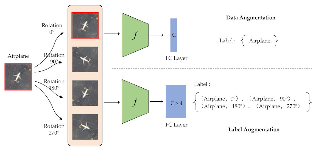
In Figure 1, we take the rotation transformations of a sample as an example to show the difference between data augmentation and label augmentation. We rotate the original image by 0°, 90°, 180° and 270° to generate four images. When we use data augmentation, all 4 images are labeled with the category airplane. When using label augmentation, the rotation information is added to the label. In this manner, a joint label for each generated image can be obtained [44]. Therefore, the category is expanded four-fold. The labels of four images are (airplane, 0°), (airplane, 90°), (airplane, 180°) and (airplane, 270°). Label augmentation can make each remote sensing image obtain more accurate category information than data augmentation.
With the increase in categories, the design of the classifier needs to be adjusted. We use to represent a training sample, and it has a label , where is the number of categories. When we use data augmentation, the loss function can be expressed as:
where is obtained by applying the rotation transformation to the original training sample . represents the cross-entropy loss function, and represents the parameters of network .
However, when applying the label augmentation, the joint label is used to increase category information, and the loss function of label augmentation can be expressed as:
where is the number of images obtained by label augmentation. In Figure 1, we use 4 rotation transformations to obtain 4 images, so is equal to 4. There is a 4-fold increase in categories, so the dimension of the fully connected layer (FC) is also expanded 4-fold to .
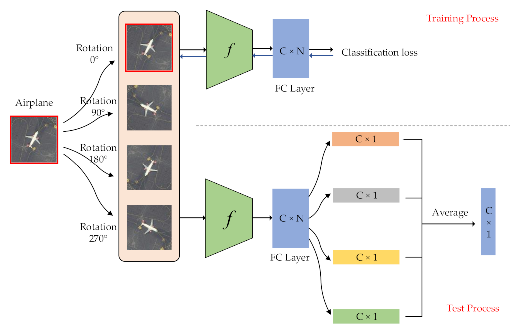
We show the training and test process of the label augmentation in Figure 2. During the training process, we train the model using the standard cross-entropy loss and update the parameters of the network using a backpropagation algorithm. During the test process, we first aggregate outputs by calculating the average of output vectors as follows:
Then, we can calculate the softmax probability by:
With the label augmentation, we can use a single CNN model to identify scene category and rotation transformation at the same time, which fully uses the training set to enhance classification performance.
2.2. Intra-Class Constraint for RS Image Scene Classification
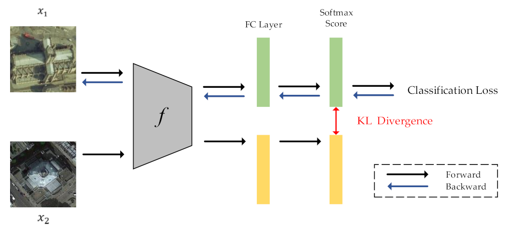
Although label augmentation can provide more training samples having accurate category information, it also increases the intra-class diversity among the training set. The intra-class diversity has an important influence on test accuracy. To address this issue, we utilize KL divergence as a regularization term to impose intra-constraint. In detail, we input two training samples with the same category into the network and obtain their output distribution. Since the input images have the same category, their output distribution should be similar. Therefore, we calculate the KL divergence of the two output distributions as the regularization term.
The framework of intra-class constraint is shown in Figure 3. During the training process, in addition to the current training sample , we input another randomly selected sample with the same category as sample into the network. The KL divergence is used to match the output distribution of two training samples.
The output distribution of input image is defined as follows:
where is the distillation temperature, which is used to soften the output distribution. Then, we propose the following KL divergence regularization term to impose intra-constraint:
The total loss can be obtained by combining cross-entropy loss function and KL divergence regularization term:
where represents the cross-entropy loss, and is the coefficient of the KL divergence. We set to 1 to indicate that cross-entropy loss and KL divergence regularization term have same importance in our method.
Moreover, we only perform backpropagation for the training sample . The training sample is only used to calculate the value of KL divergence, and the process of backpropagation is not necessary.
2.3. Combination of LA and Intra-Class Constraint for RS Image Scene Classification
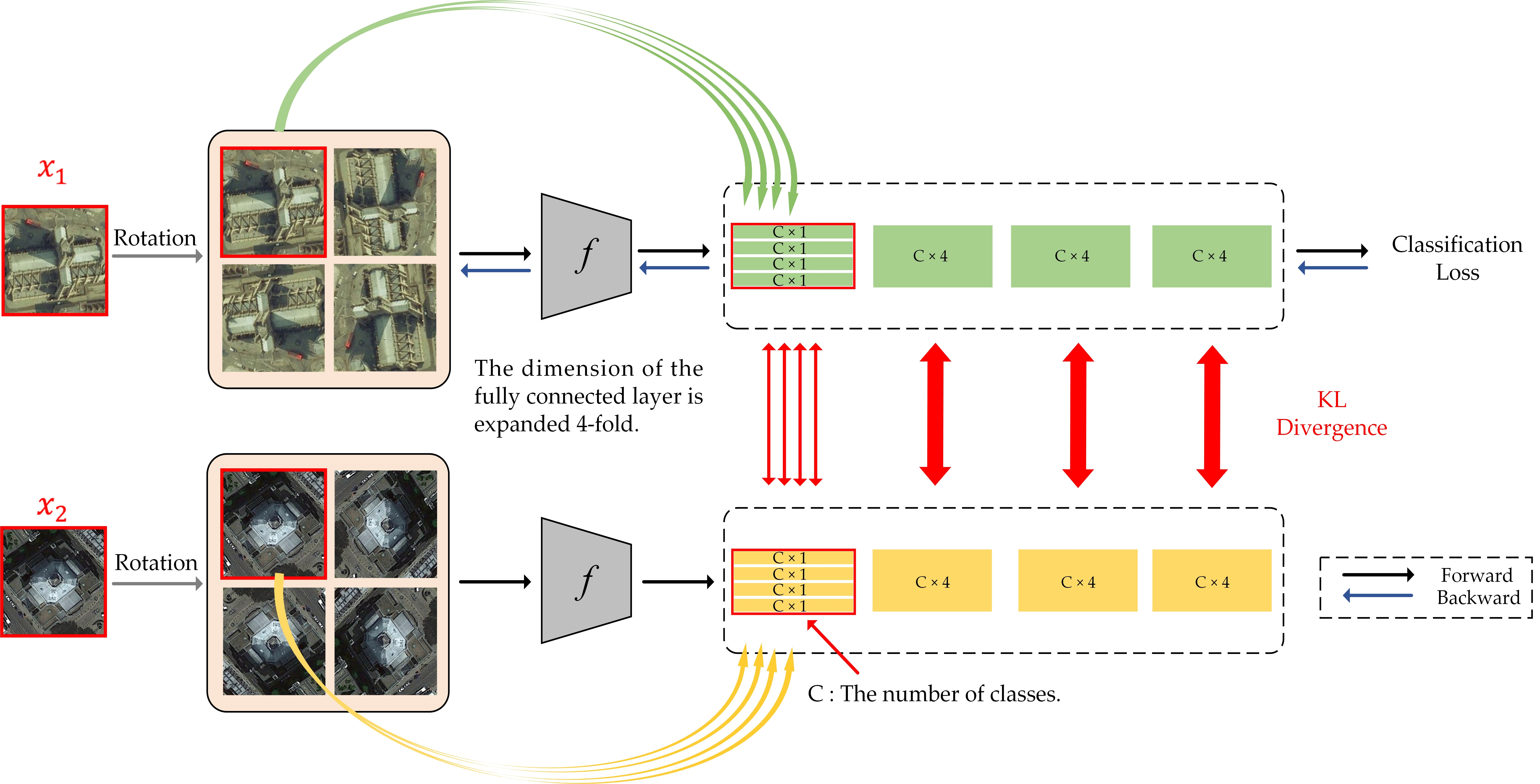
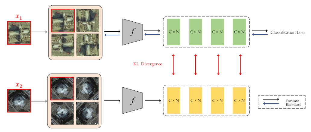
In this sub-section, we combine the above two methods, i.e., LA and Intra-class Constraint, to further enhance the classification performance. Figure 4 displays the overall framework of the proposed method.
Similar to the intra-class constraint, we have a current input image and a randomly selected image with the same category as sample . By applying label augmentation to samples and , the number of images and categories has increased by N times. As shown in Figure 4, for each input image, we use 4 rotation transformations to obtain four images with the joint label. Then, we calculate the KL divergence of these four pairs of images. The total loss can be calculated by combining loss and KL divergence:
Moreover, the backpropagation process is only for samples and its augmented samples, and the training sample is only used to calculate the value of KL divergence.
Algorithm 1 shows the workflow of the proposed method. The combination of label augmentation and intra-class constraint enables us to fully use the training set to enhance the classification performance.
| Algorithm 1: The workflow of label augmentation and intra-class constraint. |
| 1. begin |
| 2. randomly select the RS images to generate the training set and test set |
| 3. initialize the model with the parameters w of the model pre-trained on the ImageNet |
| 4. Train model: |
| 5. for epoch in 1: epochs: |
| 6. sample a batch (x, y) from the training set |
| 7. sample another batch (, y) with the same category y from the training set |
| 8. apply LA to each image in two batches to generate four new images and their joint labels |
| 9. calculate the cross-entropy loss |
| 10. obtain output distributions of the two samples with the same location in two batches |
| 11. calculate the KL divergence of two output distributions |
| 12. update parameters w by minimizing the loss |
| 10. Test: |
| 11. apply LA to each image in the test set |
| 12. output = model (test image) |
| 13. aggregate the output and calculate the softmax probability |
| 14. end |
3. Experiments
3.1. Datasets Description
In order to verify the effectiveness of the label augmentation and intra-class constraint, we carry out experiments on three public RS image datasets: the UC Merced (UCM) dataset [14], the AID dataset [45] and the NWPU-RESISC45 dataset [28].
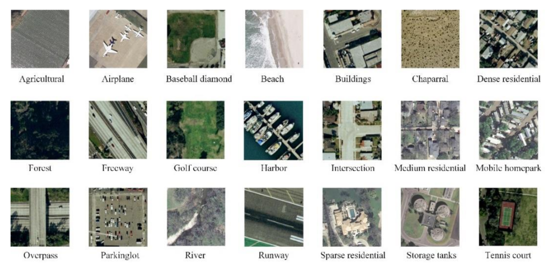
The UCM dataset contains 2100 remote sensing images and is divided into 21 scene categories. There are 100 images in each category, and each image consists of 256 × 256 pixels, and the spatial resolution is 0.3 m. Figure 5 shows some selected images and their corresponding scene categories.
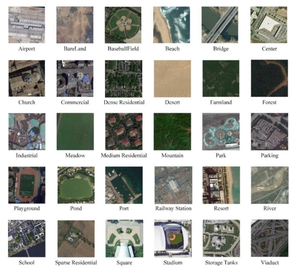
The AID dataset consists of 10,000 remote sensing images, which are assigned to 30 scene categories. Each scene contains between 220 and 420 images. Each image has 600 × 600 pixels, and the spatial resolution is between 8 m and 0.5 m. Some selected images and their corresponding scene categories are shown in Figure 6.
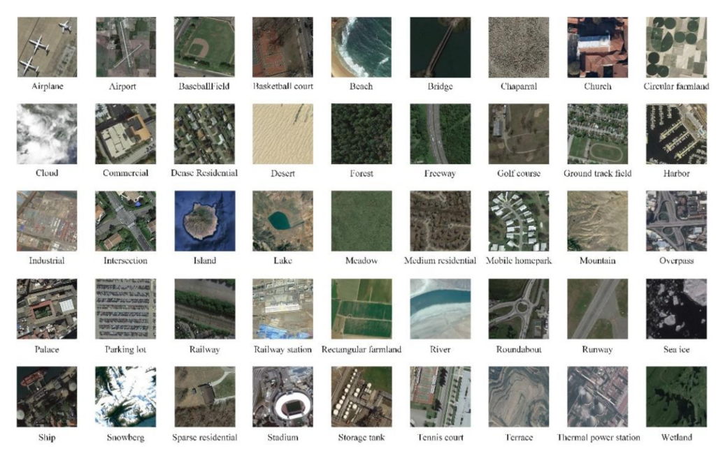
The NWPU-RESISC45 dataset is collected from Google Earth, and it contains 31,500 images, all of which have 256 × 256 pixels. These RS images belong to 45 scene categories. There are 700 images in each category, and the spatial resolution is between 30 m and 0.2 m. Some images and their corresponding scene categories are displayed in Figure 7.
3.2. Experimental Setup
For the UCM dataset, we select 80% of images to create a training set. For the AID dataset, we use 20% and 50% training ratios to create a training set. The training ratio of the NWPU-RESISC45 dataset is set to 10% and 20%. For the above three datasets, samples other than the training set constitute the test set.
The overall accuracy (OA) and confusion matrix are used to evaluate the performance of the proposed method. The OA reflects the classification performance of the CNN model. The confusion matrix is a way of accuracy evaluation. It is expressed in a matrix with rows and columns, where represents the number of scene categories in each dataset. The confusion matrix reflects the relationship between the predicted result and label, and the number of correctly classified images is distributed diagonally in the confusion matrix.
We select the ResNet18 model [32], which is pretrained on ImageNet, as the backbone network. The last fully connected layer of the pretrained ResNet18 model is replaced with a new fully connected layer which is used to obtain the final classification results of the RS image classification task. In the experiments, two label augmentation (LA) methods are used, including color permutation and rotation. For the rotation operation, the rotation angles are set to 0, 90, 180 and 270 degrees. For the color permutation, there are three transformations, including RGB, GBR and BRG.
In the training stage, we first resize all images to 224 × 224 and then feed them into the network. Then, the stochastic gradient descent (SGD) is used to update the model parameters with a batch size of 32. We set the training epochs and initial learning rate to 40 and 0.01, respectively. In addition, as the training progresses, the learning rate gradually decreases.
We carry out the experiments on the Windows 10 system with a 3.4GHz i5-7500CPU and an NVIDIA GeForce GTX 1070Ti GPU. The PyTorch [46] open-source framework and python programming language are used to implement the proposed methods.
3.3. Experimental Results
3.3.1. Results of the AID Dataset
Since label augmentation can be considered as an improvement of the data augmentation, we first compared the label augmentation with data augmentation. We ran experiments five times with the random training set to obtain the final test results with the form of accuracy ± standard deviation. In Table 1, when using a 20% and 50% training ratio, the test results of data augmentation using color permutation were lower than fine-tuned ResNet18 by 1.65% and 0.75%, respectively. However, when applying label augmentation to color permutation, it had an improvement of 1.17% and 1.18% in terms of classification accuracy over the fine-tuned ResNet18, respectively. The above results indicated that the remote sensing images are sensitive to color permutation, and it is improper to directly assign the original label to the new image generated by the color permutation. The color transformation changed the content of the image, which increased the complexity of the classification task.
The results of label augmentation, including color permutation and rotation, were better than data augmentation, which indicates that it is reasonable to assign a joint label to each newly generated remote sensing image. The joint label can consider scene category and transformation at the same time and provide more accurate category information to improve the classification accuracy.
In detail, the classification accuracy of LA with rotation transformation was higher than color permutation, which demonstrates that providing more direction and position information for the network can promote the improvement of classification accuracy. Therefore, in the following two datasets, UCM and NWPU-RESISC45, rotation transformation will be used as the way of label augmentation.
In addition, aiming at the problem of intra-class diversity caused by label augmentation, we utilized KL divergence to constrain the output distribution of different samples with the same scene category. In addition to combining ResNet18 + LA with KL divergence, we conducted an ablation study to explore the effect of using KL divergence alone on ResNet18. The experimental results are shown in Table 2.
When applying KL divergence to ResNet18 and ResNet18 + LA, it has an improvement of 0.62% and 0.85% in terms of classification accuracy, using a 20% training ratio, respectively. When using a 50% training ratio, the results show a similar trend, which proves the effectiveness of using KL divergence to constrain intra-class diversity among training sets.
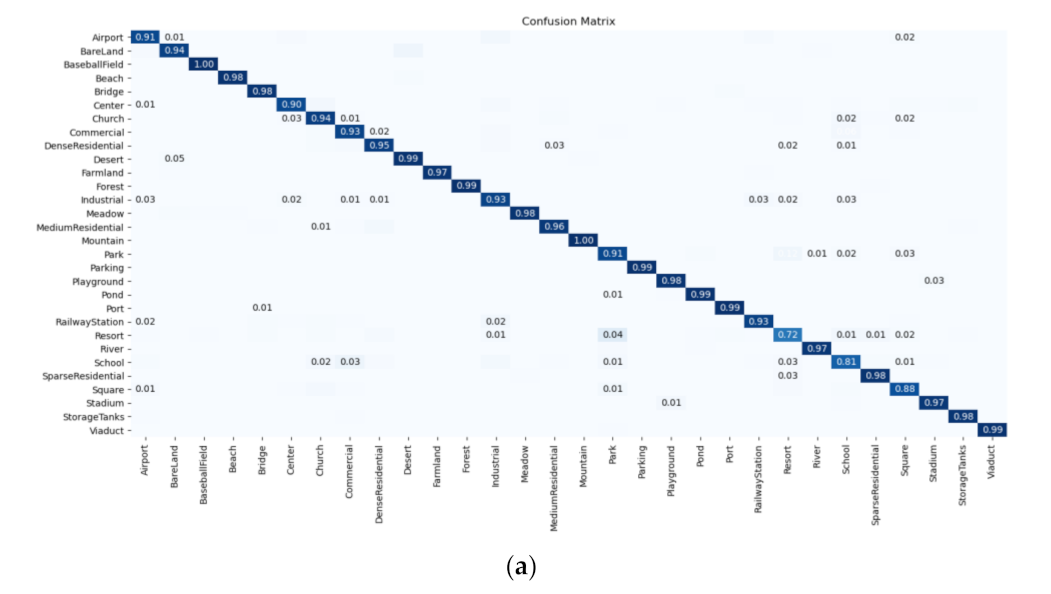
Figure 8 shows the confusion matrices of the ResNet18 + LA (rotation) + KL for the AID dataset. One can see that the correctly classified test samples are distributed diagonally in the two confusion matrices, and most scenes can be classified with an accuracy of more than 90%.
Table 3 shows the comparison of our results with other advanced methods. One can see that our proposed method, ResNet18 + LA (rotation) + KL, achieved 94.98% and 96.52% classification accuracy, under the training ratio of 20% and 50%, respectively, which is higher than most previous methods. Rotation Invariance Regularization (RIR) [47] proposes a deep Siamese CNN with rotation invariance regularization that combines a regularization constraint with the cross-entropy loss, which can obtain results similar to our method.
3.3.2. Results of UCM Dataset
According to Table 4, by combining KL divergence with ResNet18 and ResNet18 + LA, it has an enhancement of 1.16% and 0.24% in terms of test accuracy, under the training ratio of 80%, respectively. Compared with data augmentation, the improvement obtained by the label augmentation is 0.75%. Moreover, the ResNet18 + LA (rotation) + KL can achieve the highest classification accuracy of 99.21%.
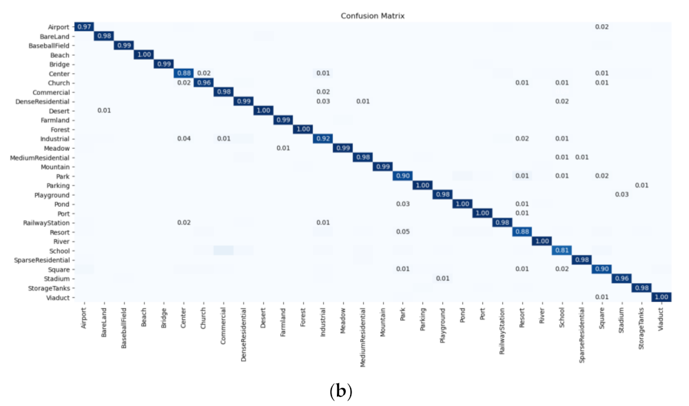
As can be seen from the confusion matrices in Figure 9, every scene can be easily distinguished from the others, and almost all categories can be correctly identified with the classification accuracy of 1. For some categories that are easy to confuse, such as Overpass and Freeway, after applying the KL divergence, the classification accuracy of category Freeway has an improvement of 5%. These results demonstrate that the ResNet18 + LA + KL improves the overall accuracy by imposing KL divergence on the output distributions.
The overall classification comparison on the UCM is displayed in Table 5. The classification accuracy of 99.21% can be obtained by the proposed method ResNet18 + LA (rotation) + KL, which is higher than most previous methods. DCNN [46] also solves the problem of intra-class diversity among remote sensing images by metric learning, and RIR [48] uses the rotation transformation and Siamese CNN to increase the robustness for the remote sensing images scene classification. The combination of label augmentation and intra-class constraint is superior to the above two methods. However, our classification performance is slightly lower than method ACNet [37] that uses the dual-branch structure and attention technique.
3.3.3. Results of the NWPU Dataset
The results of the label augmentation and intra-class constraint are given in Table 6. Similar to the experimental results of the above two datasets, the method ResNet18 + LA (rotation) and ResNet18 + LA (rotation) + KL achieve higher classification accuracy than baseline, which validates the effectiveness and robustness of our proposed methods.
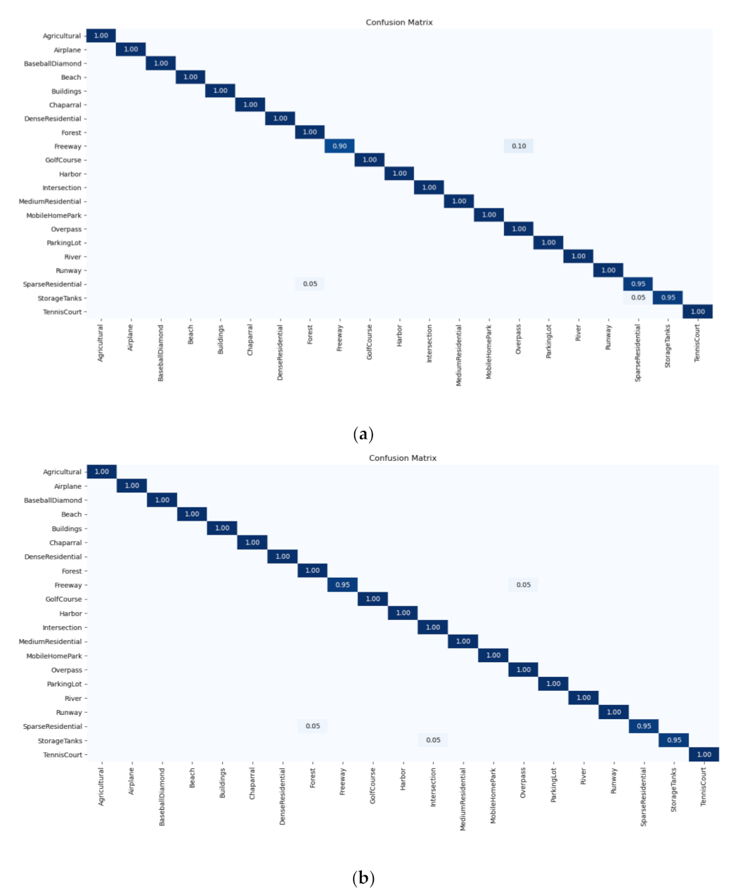
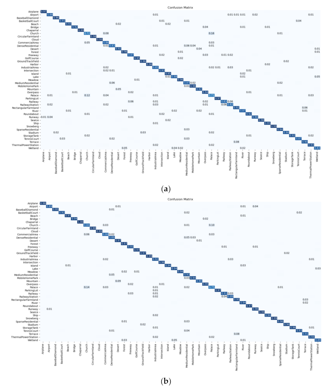
It is clear that the number of correctly classified images is distributed diagonally in the confusion matrix in Figure 10. According to Table 7, by combining the label augmentation and KL divergence, we can obtain 91.05% and 93.60% classification accuracy, using 10% and 20% training ratios, respectively. Moreover, the ResNet18 + LA (rotation) + KL shows an excellent classification performance than most methods in Table 7.
4. Discussion
4.1. Experimental Analysis
As can be seen from the results of the AID dataset and the NWPU dataset, the classification accuracy has an improvement with the increase in the training ratio, indicating that the number of training sets has an important influence on the training model. The label augmentation proposed in this paper assigns a joint label to each new image obtained by the input transformation, i.e., rotation transformation. By applying the label augmentation, we can obtain more accurate category information and make the model use the training samples more effectively, which significantly improves the classification accuracy. In addition, by using KL divergence to constrain the output distribution of the two images with the same category, the classification performance can be further improved, indicating that the use of KL divergence can solve the problem of intra-class diversity caused by label augmentation to some extent. We also compare our methods with other advanced methods. DCNN [46] uses metric learning to solve the problem of intra-class diversity among remote sensing images. RIR [48] uses the rotation transformation and Siamese CNN to increase the robustness of the CNN model. The ResNet18 + LA + KL achieves the highest classification results in most cases compared with the above two methods, which validates the effectiveness of our method.
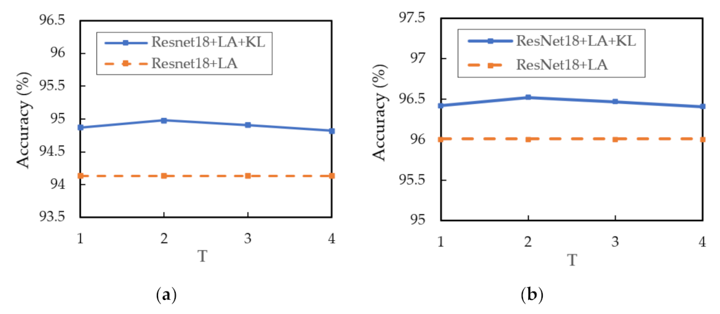
4.2. Parameter Sensitivity Analysis
The influence of the factor on KL divergence is analyzed. The factor is an important parameter, which decides the soft degree of the output distribution. We set the value of as {1, 2, 3, 4} and conduct experiments on the AID dataset.
In Figure 11, when the value of is set to 2, the ResNet18 + LA + KL obtains the highest test accuracy.
4.3. Analysis of Softmax Scores
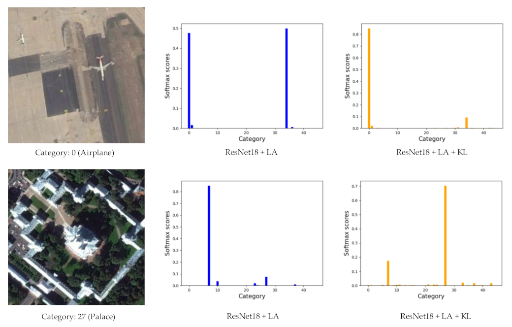
The softmax scores reflect the probability of the image belonging to each category. We use a bar chart to display the softmax scores. Figure 12 shows the softmax scores of two test samples obtained by ResNet18 + LA and ResNet18 + LA + KL. The first test sample belongs to category 0 (airplane), but the prediction obtained by ResNet18 + LA is category 34 (runway). The reason is that the airplane area occupies a small proportion of the image, while the runway area occupies most of the image. Therefore, it is easy to confuse this image with category runway.
When applying KL divergence, we can provide the constraint on output distribution, and the prediction obtained by ResNet18 + LA is category 0 (airplane), which is the correct result. The second test sample belongs to category 27 (palace), and it is similar to category 7 (church). We can see that the prediction of ResNet18 + LA + KL obtains the correct classification result.
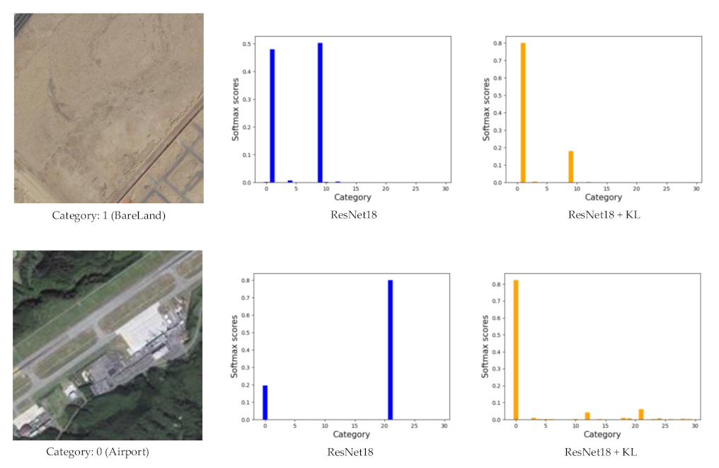
The softmax scores of two test samples obtained by ResNet18 and ResNet18 + KL are shown in Figure 13. By using the KL divergence to impose constraint, the intra-class diversity is decreased, which results in the indirect decrease in between-class similarity. The first test sample in Figure 13 belongs to category 1 (bareland). One can see that the probabilities of bareland and desert obtained by ResNet18 are close, indicating that it is easy to confuse bareland and desert. When the KL divergence is applied to ResNet18, the distance between feature distributions of different categories is increased due to the intra-class constraints, and the prediction of ResNet18 + KL obtains the correct classification result. The result of the second test sample has the same trend. The results in Figure 12 and Figure 13 validate the effectiveness of using the KL divergence.
4.4. Analysis of the Comparsion Experiment
We use the same data augmentation strategy and the same model to give a fair comparison. In the comparison experiments, the RIR [48] also uses the same rotation operation to expand the training set. In the case of using the same model (e.g., ResNet50), we compare our results with the RIR [48] on the NWPU dataset. The results are shown in Table 8.
We can obtain 93.37% and 95.26% classification accuracy by the ResNet50, using 10% and 20% training ratios, respectively. Compared with the RIR [49], it has an enhancement of 1.32% and 1.2% in terms of classification accuracy, which proves the effectiveness of the proposed method.
4.5. Analysis of Running Time and Computational Complexity
In order to analyze the computational cost of the proposed method, we conduct the following four experiments on the AID dataset: ResNet18, ResNet18 + DA (rotation), ResNet18 + LA (rotation), and ResNet18 + LA (rotation) + KL. The experimental results are shown in Table 9.
From Table 9, one can see that the application of data augmentation does not significantly increase the training time since data augmentation does not change the total number of training samples. When we use the label augmentation, there is a four-fold increase in training samples, and the dimension of the fully connected layer is also expanded four-fold. Therefore, the training time is longer than the data augmentation due to the increase in training samples and network parameters.
We calculate the number of floating-point operations (FLOPs) for different models. The number of FLOPs on ResNet18 and ResNet18 + DA (rotation) is 1820.90 M. However, when we use the label augmentation, the dimension of the fully connected layer is expanded four-fold. Therefore, the number of FLOPs on ResNet18 + LA (rotation) is increased to 1820.95 M. For the ResNet18 + LA (rotation) + KL, the network needs to calculate the output of two samples with the same category, so the number of FLOPs on ResNet18 + LA (rotation) + KL is 3641.90 M.
We also calculate the number of parameters in the model. For the ResNet18 and ResNet18 + DA (rotation), the last fully connected layer of the pretrained ResNet18 model is replaced with a new fully connected layer which is used to obtain the final classification results of the RS image classification task. The number of parameters in ResNet18 and ResNet18 + DA (rotation) is 11.19 M. For the ResNet18 + LA (rotation) and ResNet18 + LA (rotation) + KL, the dimension of the fully connected layer is expanded four-fold. Therefore, the number of parameters in ResNet18 + LA (rotation) and ResNet18 + LA (rotation) + KL is increased to 11.24 M.
4.6. Discussion of the Generalization Ability of the Proposed Method
Considering that the label augmentation uses four fixed rotation angles (e.g., 0°, 90°, 180° and 270°) to expand the training set, we introduce a small random angle α for four fixed rotation angles to increase the generalization ability of the network, which is called improved label augmentation (ILA). In addition, we double the number of samples for each rotation angle (e.g., 0° ± α, 90° ± α, 180° ± α and 270° ± α) to further expand the training set. In the experiments, the small random angle α is set to 10. The results on the NWPU dataset are shown in Table 10.
From Table 10, when using the improved label augmentation, we can obtain 91.81% and 93.91% classification accuracy, using 10% and 20% training ratios, respectively. Compared with the ResNet18 + LA (rotation) + KL, it has an enhancement of 0.76% and 0.31% in terms of classification accuracy. The above results demonstrated that the improved label augmentation could enhance the generalization ability of the network to further improve the classification performance.
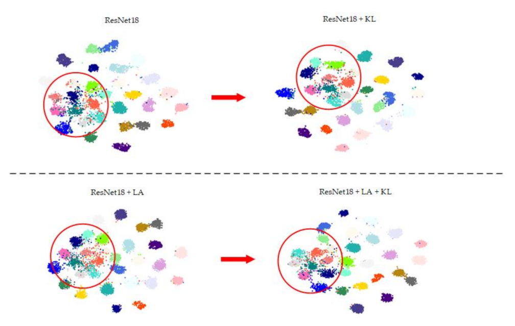
4.7. Visualization of Feature Embeddings Using T-SNE
The T-SNE algorithm can map the features in the high-dimensional space to the low-dimensional space while retaining the characteristics of features [51]. We extract the 512-dimensional feature vector from the penultimate layer of the network, and then we map it to 2-dimension space. Figure 14 shows the T-SNE result of different methods on the AID dataset with a 20% training ratio. In Figure 14, each color represents a scene category, and one can see that the distinguishability between categories is increased by using KL divergence.
5. Conclusions
In this study, how to efficiently use remote sensing images to address the scene classification task was explored, and then label augmentation and intra-class constraint were proposed to improve the classification performance. We selected ResNet18 as the backbone network to perform experiments on the three RS datasets. By applying label augmentation, we considered the label and data augmentation at the same time, which can obtain higher classification accuracy than data augmentation. Then, KL divergence was used to solve the intra-class diversity caused by label augmentation. The combination of label augmentation and intra-class constraint was superior to other excellent methods in classification accuracy. The experimental results in this paper demonstrated that great performance gains could be obtained by making full use of data even without complex algorithms. There is great prospect to study how to improve scene classification performance from the data level.
Author Contributions
Conceptualization, Y.C.; methodology, H.X. and Y.C.; writing—original draft preparation, H.X., Y.C. and P.G. All authors have read and agreed to the published version of the manuscript.
Funding
This research was funded by the Natural Science Foundation of China under grants 61971164 and U20B2041.
Conflicts of Interest
The authors declare no conflict of interest.
References
- Cheng, G.; Han, J.; Zhou, P.; Guo, L. Multi-class geospatial object detection and geographic image classification based on collection of part detectors. ISPRS J. Photogramm. Remote Sens. 2014, 98, 119–132. [Google Scholar] [CrossRef]
- Cheng, G.; Han, J. A survey on object detection in optical remote sensing images. ISPRS J. Photogramm. Remote Sens. 2016, 117, 11–28. [Google Scholar] [CrossRef] [Green Version]
- Han, J.; Zhang, D.; Cheng, G.; Guo, L.; Ren, J. Object detection in optical remote sensing images based on weakly supervised learning and high-level feature learning. IEEE Trans. Geosci. Remote Sens. 2014, 53, 3325–3337. [Google Scholar] [CrossRef] [Green Version]
- Aptoula, E. Remote sensing image retrieval with global morphological texture descriptors. IEEE Trans. Geosci. Remote Sens. 2014, 52, 3023–3034. [Google Scholar] [CrossRef]
- Yang, Y.; Newsam, S. Geographic image retrieval using local invariant features. IEEE Trans. Geosci. Remote Sens. 2013, 52, 818–832. [Google Scholar] [CrossRef]
- Shi, W.; Zhang, M.; Zhang, R.; Chen, S.; Zhan, Z. Change detection based on artificial intelligence: State-of-the-art and challenges. Remote Sens. 2020, 12, 1688. [Google Scholar] [CrossRef]
- Peng, D.; Zhang, Y.; Guan, H. End-to-end change detection for high resolution satellite images using improved UNet++. Remote Sens. 2019, 11, 1382. [Google Scholar] [CrossRef] [Green Version]
- Castelluccio, M.; Poggi, G.; Sansone, C.; Verdoliva, L. Land use classification in remote sensing images by convolutional neural networks. arXiv 2015, arXiv:1508.00092. [Google Scholar]
- Manfreda, S.; McCabe, M.F.; Miller, P.E.; Lucas, R.; Pajuelo Madrigal, V.; Mallinis, G.; Ben Dor, E.; Helman, D.; Estes, L.; Ciraolo, G.; et al. On the use of unmanned aerial systems for environmental monitoring. Remote Sens. 2018, 10, 641. [Google Scholar] [CrossRef] [Green Version]
- Swain, M.J.; Ballard, D.H. Color indexing. Int. J. Comput. Vis. 1991, 7, 11–32. [Google Scholar] [CrossRef]
- Ojala, T.; Pietikainen, M.; Maenpaa, T. Multiresolution gray-scale and rotation invariant texture classification with local binary patterns. IEEE Trans. Pattern Anal. Mach. Intell. 2002, 24, 971–987. [Google Scholar] [CrossRef]
- Haralick, R.M.; Shanmugam, K.; Dinstein, I.H. Textural features for image classification. IEEE Trans. Syst. Man Cybern. 1973, 3, 610–621. [Google Scholar] [CrossRef] [Green Version]
- Lowe, D.G. Distinctive image features from scale-invariant keypoints. Int. J. Comput. Vis. 2004, 60, 91–110. [Google Scholar] [CrossRef]
- Yang, Y.; Newsam, S. Bag-of-visual-words and spatial extensions for land-use classification. In Proceedings of the 18th SIGSPATIAL International Conference on Advances in Geographic Information Systems, San Jose, CA, USA, 2–5 November 2010; pp. 270–279. [Google Scholar]
- Zhu, Q.; Zhong, Y.; Zhao, B.; Xia, G.S.; Zhang, L. Bag-of-visual-words scene classifier with local and global features for high spatial resolution remote sensing imagery. IEEE Geosci. Remote Sens. Lett. 2016, 13, 747–751. [Google Scholar] [CrossRef]
- Zhao, L.J.; Tang, P.; Huo, L.Z. Land-use scene classification using a concentric circle-structured multiscale bag-of-visual-words model. IEEE J. Sel. Top. Appl. Earth Ob. Remote Sens. 2014, 7, 4620–4631. [Google Scholar] [CrossRef]
- Zhao, B.; Zhong, Y.; Zhang, L. A spectral–structural bag-of-features scene classifier for very high spatial resolution remote sensing imagery. ISPRS J. Photogramm. Remote Sens. 2016, 116, 73–85. [Google Scholar] [CrossRef]
- Lazebnik, S.; Schmid, C.; Ponce, J. Beyond bags of features: Spatial pyramid matching for recognizing natural scene categories. In Proceedings of the IEEE Conference on Computer Vision and Pattern Recognition, New York, NY, USA, 17–22 June 2006; pp. 2169–2178. [Google Scholar]
- Perronnin, F.; Sánchez, J.; Mensink, T. Improving the fisher kernel for large-scale image classification. In Proceedings of the European Conference on Computer Vision, Heraklion, Crete, Greece, 5–11 September 2010; pp. 143–156. [Google Scholar]
- Jegou, H.; Perronnin, F.; Douze, M.; Sánchez, J.; Perez, P.; Schmid, C. Aggregating local image descriptors into compact codes. IEEE Trans. Pattern Anal. Mach. Intell. 2012, 34, 1704–1716. [Google Scholar] [CrossRef] [Green Version]
- Zhang, L.; Zhang, L.; Du, B. Deep learning for remote sensing data: A technical tutorial on the state of the art. IEEE Geosci. Remote Sens. Mag. 2016, 4, 22–40. [Google Scholar] [CrossRef]
- Chen, J.; Wang, C.; Ma, Z.; Chen, J.; He, D.; Ackland, S. Remote sensing scene classification based on convolutional neural networks pre-trained using attention-guided sparse filters. Remote Sens. 2018, 10, 290. [Google Scholar] [CrossRef] [Green Version]
- Penatti, O.A.; Nogueira, K.; dos Santos, J.A. Do deep features generalize from everyday objects to remote sensing and aerial scenes domains? In Proceedings of the IEEE Conference on Computer Vision and Pattern Recognition Workshops, Boston, MA, USA, 7–12 June 2015; pp. 44–51. [Google Scholar]
- Hu, F.; Xia, G.S.; Hu, J.; Zhang, L. Transferring deep convolutional neural networks for the scene classification of high-resolution remote sensing imagery. Remote Sens. 2015, 7, 14680–14707. [Google Scholar] [CrossRef] [Green Version]
- Marmanis, D.; Datcu, M.; Esch, T.; Stilla, U. Deep learning earth observation classification using ImageNet pretrained networks. IEEE Geosci. Remote Sens. Lett. 2015, 13, 105–109. [Google Scholar] [CrossRef] [Green Version]
- Zhang, Y.; Zheng, X.; Yuan, Y.; Lu, X. Attribute-cooperated convolutional neural network for remote sensing image classification. IEEE Trans. Geosci. Remote Sens. 2020, 58, 8358–8371. [Google Scholar] [CrossRef]
- Li, F.; Feng, R.; Han, W.; Wang, L. High-resolution remote sensing image scene classification via key filter bank based on convolutional neural network. IEEE Trans. Geosci. Remote Sens. 2020, 58, 8077–8092. [Google Scholar] [CrossRef]
- Cheng, G.; Han, J.; Lu, X. Remote sensing image scene classification: Benchmark and state of the art. Proc. IEEE 2017, 105, 1865–1883. [Google Scholar] [CrossRef] [Green Version]
- Deng, J.; Dong, W.; Socher, R.; Li, L.J.; Li, K.; Li, F.-F. ImageNet: A large-scale hierarchical image database. In Proceedings of the IEEE Conference on Computer Vision and Pattern Recognition, Miami, FL, USA, 20–25 June 2009; pp. 248–255. [Google Scholar]
- Krizhevsky, A.; Sutskever, I.; Hinton, G.E. Imagenet classification with deep convolutional neural networks. In Proceedings of the Advances in Neural Information Processing Systems, Lake Tahoe, NV, USA, 3–8 December 2012; pp. 1097–1105. [Google Scholar]
- Simonyan, K.; Zisserman, A. Very deep convolutional networks for large-scale image recognition. arXiv 2014, arXiv:1409.1556. [Google Scholar]
- He, K.; Zhang, X.; Ren, S.; Sun, J. Deep residual learning for image recognition. In Proceedings of the IEEE Conference on Computer Vision and Pattern Recognition, Las Vegas, NV, USA, 27 June 2016; pp. 770–778. [Google Scholar]
- Huang, G.; Liu, Z.; Van Der Maaten, L.; Weinberger, K.Q. Densely connected convolutional networks. In Proceedings of the IEEE Conference on Computer Vision and Pattern Recognition, Honolulu, HI, USA, 21–26 July 2017; pp. 4700–4708. [Google Scholar]
- Nogueira, K.; Penatti, O.A.; dos Santos, J.A. Towards better exploiting convolutional neural networks for remote sensing scene classification. Pattern Recognit. 2017, 61, 539–556. [Google Scholar] [CrossRef] [Green Version]
- Bi, Q.; Qin, K.; Zhang, H.; Xie, J.; Li, Z.; Xu, K. APDC-Net: Attention pooling-based convolutional network for aerial scene classification. IEEE Geosci. Remote. Sens. Lett. 2019, 17, 1603–1607. [Google Scholar] [CrossRef]
- Wang, Q.; Liu, S.; Chanussot, J.; Li, X. Scene classification with recurrent attention of VHR remote sensing images. IEEE Trans. Geosci. Remote Sens. 2018, 57, 1155–1167. [Google Scholar] [CrossRef]
- Tang, X.; Ma, Q.; Zhang, X.; Liu, F.; Ma, J.; Jiao, L. Attention consistent network for remote sensing scene classification. IEEE J. Sel. Top. Appl. Earth Ob. Remote Sens. 2021, 14, 2030–2045. [Google Scholar] [CrossRef]
- Guo, Y.; Ji, J.; Lu, X.; Huo, H.; Fang, T.; Li, D. Global-local attention network for aerial scene classification. IEEE Access 2019, 7, 67200–67212. [Google Scholar] [CrossRef]
- Zhong, Y.; Zhu, Q.; Zhang, L. Scene classification based on the multifeature fusion probabilistic topic model for high spatial resolution remote sensing imagery. IEEE Trans. Geosci. Remote Sens. 2015, 53, 6207–6222. [Google Scholar] [CrossRef]
- Yu, Y.; Liu, F. Dense connectivity based two-stream deep feature fusion framework for aerial scene classification. Remote Sens. 2018, 10, 1158. [Google Scholar] [CrossRef] [Green Version]
- Chaib, S.; Liu, H.; Gu, Y.; Yao, H. Deep feature fusion for VHR remote sensing scene classification. IEEE Trans. Geosci. Remote Sens. 2017, 55, 4775–4784. [Google Scholar] [CrossRef]
- Lu, X.; Sun, H.; Zheng, X. A feature aggregation convolutional neural network for remote sensing scene classification. IEEE Trans. Geosci. Remote Sens. 2019, 57, 7894–7906. [Google Scholar] [CrossRef]
- Wang, G.; Fan, B.; Xiang, S.; Pan, C. Aggregating rich hierarchical features for scene classification in remote sensing imagery. IEEE J. Sel. Top. Appl. Earth Ob. Remote Sens. 2017, 10, 4104–4115. [Google Scholar] [CrossRef]
- Lee, H.; Hwang, S.J.; Shin, J. Self-supervised Label Augmentation via Input Transformations. arXiv 2019, arXiv:1910.05872. [Google Scholar]
- Xia, G.S.; Hu, J.; Hu, F.; Shi, B.; Bai, X.; Zhong, Y.; Zhang, L.; Lu, X. AID: A benchmark data set for performance evaluation of aerial scene classification. IEEE Trans. Geosci. Remote Sens. 2017, 55, 3965–3981. [Google Scholar] [CrossRef] [Green Version]
- Paszke, A.; Gross, S.; Massa, F.; Lerer, A.; Bradbury, J.; Chanan, G.; Killeen, T.; Lin, Z.; Gimelshein, N.; Antiga, L.; et al. PyTorch: An imperative style, high-performance deep learning library. In Proceedings of the 32th International Conference on Neural Information Processing Systems, Vancouver, BC, Canada, 8–14 December 2019; pp. 8024–8035. [Google Scholar]
- Cheng, G.; Yang, C.; Yao, X.; Guo, L.; Han, J. When deep learning meets metric learning: Remote sensing image scene classification via learning discriminative CNNs. IEEE Trans. Geosci. Remote Sens. 2018, 56, 2811–2821. [Google Scholar] [CrossRef]
- Zhang, W.; Tang, P.; Zhao, L. Remote sensing image scene classification using CNN-CapsNet. Remote Sens. 2019, 11, 494. [Google Scholar] [CrossRef] [Green Version]
- Qi, K.; Yang, C.; Hu, C.; Shen, Y.; Shen, S.; Wu, H. Rotation invariance regularization for remote sensing image scene classification with convolutional neural networks. Remote Sens. 2021, 13, 569. [Google Scholar] [CrossRef]
- Liu, X.; Zhou, Y.; Zhao, J.; Yao, R.; Liu, B.; Zheng, Y. Siamese convolutional neural networks for remote sensing scene classification. IEEE Geosci. Remote. Sens. Lett. 2019, 16, 1200–1204. [Google Scholar] [CrossRef]
- Maaten, L.; Hinton, G. Visualizing data using t-SNE. J. Mach. Learn. Res. 2008, 9, 2579–2605. [Google Scholar]
Figure 1.
The difference between data augmentation and label augmentation.

Figure 2.
The training and test process of label augmentation.

Figure 3.
The framework of the intra-class constraint.

Figure 4.
The framework of the combination of label augmentation and intra-class constraint.

Figure 5.
The UCM dataset.

Figure 6.
The AID dataset.

Figure 7.
The NWPU-RESISC45 dataset.

Figure 8.
Confusion matrices of the ResNet18 + LA (rotation) + KL for the AID dataset, using (a) 20% and (b) 50% training ratios.
Figure 8.
Confusion matrices of the ResNet18 + LA (rotation) + KL for the AID dataset, using (a) 20% and (b) 50% training ratios.


Figure 9.
The confusion matrix obtained by (a) ResNet18 + LA (rotation) and (b) ResNet18 + LA (rotation) + KL on the UCM dataset.
Figure 9.
The confusion matrix obtained by (a) ResNet18 + LA (rotation) and (b) ResNet18 + LA (rotation) + KL on the UCM dataset.

Figure 10.
Confusion matrices of the ResNet18 + LA (rotation) + KL for NWPU dataset, using (a) 10% and (b) 20% training ratios.
Figure 10.
Confusion matrices of the ResNet18 + LA (rotation) + KL for NWPU dataset, using (a) 10% and (b) 20% training ratios.

Figure 11.
The classification accuracy of different T values: (a) 20% training samples; (b) 50% training samples.
Figure 11.
The classification accuracy of different T values: (a) 20% training samples; (b) 50% training samples.

Figure 12.
The softmax scores of two test samples on the NWPU dataset obtained by ResNet18 +LA and ResNet18 + LA + KL. The first column is two test samples on the NWPU dataset. The second column is the softmax scores obtained by ResNet18 + LA, and the last column is the softmax scores obtained by ResNet18 + LA + KL.

Figure 13.
The softmax scores of two test samples on the AID dataset obtained by ResNet18 and ResNet18 + KL. The first column is two test samples on the AID dataset. The second column is the softmax scores obtained by ResNet18, and the last column is the softmax scores obtained by ResNet18 + KL.
Figure 13.
The softmax scores of two test samples on the AID dataset obtained by ResNet18 and ResNet18 + KL. The first column is two test samples on the AID dataset. The second column is the softmax scores obtained by ResNet18, and the last column is the softmax scores obtained by ResNet18 + KL.

Figure 14.
T-SNE visualization of different methods on the AID dataset.


Table 1.
Label augmentation overall accuracy (%) on the AID dataset. The best results are shown in bold.
Table 1.
Label augmentation overall accuracy (%) on the AID dataset. The best results are shown in bold.
| Method | Training Ratio | |
|---|---|---|
| 20% | 50% | |
| ResNet18 | 92.62 ± 0.15 | 94.35 ± 0.34 |
| ResNet18 + DA (color permutation) | 90.97 ± 0.55 | 93.60 ± 0.29 |
| ResNet18 + DA (rotation) | 93.11 ± 0.22 | 95.38 ± 0.12 |
| ResNet18 + LA (color permutation) | 93.79 ± 0.12 | 95.53 ± 0.28 |
| ResNet18 + LA (rotation) | 94.13 ± 0.17 | 96.01 ± 0.08 |
Table 2.
Reduced intra-class diversity classification accuracies (%) on the AID dataset. The best results are shown in bold.
Table 2.
Reduced intra-class diversity classification accuracies (%) on the AID dataset. The best results are shown in bold.
| Methods | Training Ratio | |
|---|---|---|
| 20% | 50% | |
| ResNet18 | 92.62 ± 0.15 | 94.35 ± 0.34 |
| ResNet18 + KL | 93.24 ± 0.33 | 95.37 ± 0.23 |
| ResNet18 + LA (rotation) | 94.13 ± 0.17 | 96.01 ± 0.08 |
| ResNet18 + LA (rotation) + KL | 94.98 ± 0.04 | 96.52 ± 0.11 |
Table 3.
A comparison with other advanced methods on AID dataset. The best results are shown in bold.
Table 3.
A comparison with other advanced methods on AID dataset. The best results are shown in bold.
| Methods | Training Ratio | |
|---|---|---|
| 20% | 50% | |
| VGG-VD16 [45] | 86.59 | 89.64 |
| DCNN [47] | 90.82 | 96.89 |
| Fusion by Addition [41] | - | 91.87 |
| ACNet [37] | 93.33 | 95.38 |
| CNN-CapsNet [48] | 93.79 | 96.32 |
| SAL-TS-Net [40] | 94.09 | 95.99 |
| RIR + ResNet50 [49] | 94.95 | 96.48 |
| ResNet18 + LA (rotation) + KL (ours) | 94.98 | 96.52 |
Table 4.
The overall accuracy (%) of the UCM dataset. The best results are shown in bold.
| Methods | Training Ratio |
|---|---|
| 80% | |
| ResNet18 | 97.92 ± 0.22 |
| ResNet18 + KL | 99.08 ± 0.21 |
| ResNet18 + DA (rotation) | 98.22 ± 0.16 |
| ResNet18 + LA (rotation) | 98.97 ± 0.11 |
| ResNet18 + LA (rotation) + KL | 99.21 ± 0.11 |
Table 5.
The overall accuracy comparison of the UCM dataset. The best results are shown in bold.
| Methods | Training Ratio |
|---|---|
| 80% | |
| BoVW (SIFT) [45] | 74.12 |
| VGG-VD16 [45] | 95.21 |
| Fusion by addition [41] | 97.42 |
| ACNet [37] | 99.76 |
| CNN-CapsNet [48] | 99.05 |
| DCNN [47] | 98.93 |
| SAL-TS-Net [40] | 98.90 |
| RIR + ResNet50 [49] | 99.15 |
| ResNet18 + LA (rotation) + KL (ours) | 99.21 |
Table 6.
The overall accuracy (%) of the label augmentation and intra-class constraint on the NWPU dataset. The best results are shown in bold.
Table 6.
The overall accuracy (%) of the label augmentation and intra-class constraint on the NWPU dataset. The best results are shown in bold.
| Methods | Training Ratio | |
|---|---|---|
| 10% | 20% | |
| ResNet18 | 87.79 ± 0.40 | 90.69 ± 0.12 |
| ResNet18 + KL | 88.86 ± 0.22 | 91.67 ± 0.11 |
| ResNet18 + DA (rotation) | 89.31 ± 0.12 | 92.15 ± 0.15 |
| ResNet18 + LA (rotation) | 90.27 ± 0.25 | 92.81 ± 0.08 |
| ResNet18 + LA (rotation) + KL | 91.05 ± 0.12 | 93.60 ± 0.11 |
Table 7.
The overall accuracy comparison of the NWPU dataset. The best results are shown in bold.
| Methods | Training Ratio | |
|---|---|---|
| 10% | 20% | |
| VGG-VD16 [28] | 87.15 | 90.36 |
| DCNN [47] | 89.22 | 91.89 |
| ACNet [37] | 91.09 | 92.42 |
| CNN-CapsNet [48] | 89.03 | 92.60 |
| Siamese ResNet50 [50] | - | 92.28 |
| SAL-TS-Net [40] | 85.02 | 87.01 |
| RIR + ResNet50 [49] | 92.05 | 94.06 |
| ResNet18 + LA (rotation) + KL (ours) | 91.05 | 93.60 |
| ResNet50 + LA (rotation) + KL (ours) | 93.37 | 95.26 |
Table 8.
The test results of the NWPU dataset. The best results are shown in bold.
| Training Ratio | Method | OA (%) |
|---|---|---|
| 10% | RIR (ResNet50) [48] | 92.05 |
| ResNet18 + LA (rotation) + KL (ours) | 91.05 | |
| ResNet50 + LA (rotation) + KL (ours) | 93.37 | |
| 20% | RIR (ResNet50) [48] | 94.06 |
| ResNet18 + LA (rotation) + KL (ours) | 93.60 | |
| ResNet50 + LA (rotation) + KL (ours) | 95.26 |
Table 9.
Time consumption on the AID dataset (20% training ratio).
| Methods | Time (min) | FLOPs | Total Params | |
|---|---|---|---|---|
| Train | Test | |||
| ResNet18 | 20.37 | 1.00 | 1820.90 M | 11.19 M |
| ResNet18 + DA (rotation) | 20.62 | 1.02 | 1820.90 M | 11.19 M |
| ResNet18 + LA (rotation) | 31.50 | 1.52 | 1820.95 M | 11.24 M |
| ResNet18 + LA (rotation) + KL | 32.73 | 1.53 | 3641.90 M | 11.24 M |
Table 10.
The overall accuracy of improved label augmentation of the NWPU dataset. The best results are shown in bold.
Table 10.
The overall accuracy of improved label augmentation of the NWPU dataset. The best results are shown in bold.
| Training Ratio | Methods | OA (%) |
|---|---|---|
| 10% | ResNet18 + LA (rotation) + KL | 91.05 |
| ResNet18 + ILA (rotation) + KL | 91.81 | |
| 20% | ResNet18 + LA (rotation) + KL | 93.60 |
| ResNet18 + ILA (rotation) + KL | 93.91 |
Publisher’s Note: MDPI stays neutral with regard to jurisdictional claims in published maps and institutional affiliations. |
© 2021 by the authors. Licensee MDPI, Basel, Switzerland. This article is an open access article distributed under the terms and conditions of the Creative Commons Attribution (CC BY) license (https://creativecommons.org/licenses/by/4.0/).
Share and Cite
MDPI and ACS Style
Xie, H.; Chen, Y.; Ghamisi, P. Remote Sensing Image Scene Classification via Label Augmentation and Intra-Class Constraint. Remote Sens. 2021, 13, 2566. https://0-doi-org.brum.beds.ac.uk/10.3390/rs13132566
AMA Style
Xie H, Chen Y, Ghamisi P. Remote Sensing Image Scene Classification via Label Augmentation and Intra-Class Constraint. Remote Sensing. 2021; 13(13):2566. https://0-doi-org.brum.beds.ac.uk/10.3390/rs13132566
Chicago/Turabian StyleXie, Hao, Yushi Chen, and Pedram Ghamisi. 2021. "Remote Sensing Image Scene Classification via Label Augmentation and Intra-Class Constraint" Remote Sensing 13, no. 13: 2566. https://0-doi-org.brum.beds.ac.uk/10.3390/rs13132566
Note that from the first issue of 2016, this journal uses article numbers instead of page numbers. See further details here.