Author Contributions
Conceptualization, J.J., C.D.C., D.E.P.T. and S.O.; methodology, S.O., C.G.-C., D.-Y.L., J.J. and A.A.; software, S.O., A.A. and J.J.; validation, S.O., J.J., D.-Y.L., C.G.-C. and J.J.; formal analysis, S.O. and J.J.; investigation, S.O., J.J., D.-Y.L., C.G.-C. and C.D.C.; resources, C.D.C., D.E.P.T. and J.J.; data curation, A.A., C.G.-C., J.C., M.F.-C., B.Z.L., D.-Y.L., A.P.C. and S.O.; writing—original draft preparation, S.O., J.J., D.-Y.L., C.G.-C., C.D.C.; writing—review and editing, S.O., J.J., D.-Y.L., C.G.-C., C.D.C., A.A., M.F.-C. and D.E.P.T.; visualization, S.O., J.J. and C.D.C.; supervision, J.J. and C.D.C.; project administration, D.E.P.T.; funding acquisition, D.E.P.T., C.D.C. and J.J.; field trial conceptualization, establishment, implementation, D.E.P.T. All authors have read and agreed to the published version of the manuscript.
Figure 1.
Study area located at the Purdue Pinney Purdue Agricultural Center (PPAC), Indiana, USA. Unmanned aircraft systems (UAS) images of research plots (Trial Tar1–4) were overlaid on a Google Map satellite image [
31].
Figure 1.
Study area located at the Purdue Pinney Purdue Agricultural Center (PPAC), Indiana, USA. Unmanned aircraft systems (UAS) images of research plots (Trial Tar1–4) were overlaid on a Google Map satellite image [
31].
Figure 2.
Tar spot treatment applied in the research plots. The number in each experimental unit is the amount of fungicide applied in l/ha. The distance between research plots was modified for visual purposes. Fungicide treatments and hybrid were withheld due to confidentiality restrictions.
Figure 2.
Tar spot treatment applied in the research plots. The number in each experimental unit is the amount of fungicide applied in l/ha. The distance between research plots was modified for visual purposes. Fungicide treatments and hybrid were withheld due to confidentiality restrictions.
Figure 3.
Spatial gridding scheme used for unmanned aircraft systems (UAS)-based crop phenotyping.
Figure 3.
Spatial gridding scheme used for unmanned aircraft systems (UAS)-based crop phenotyping.
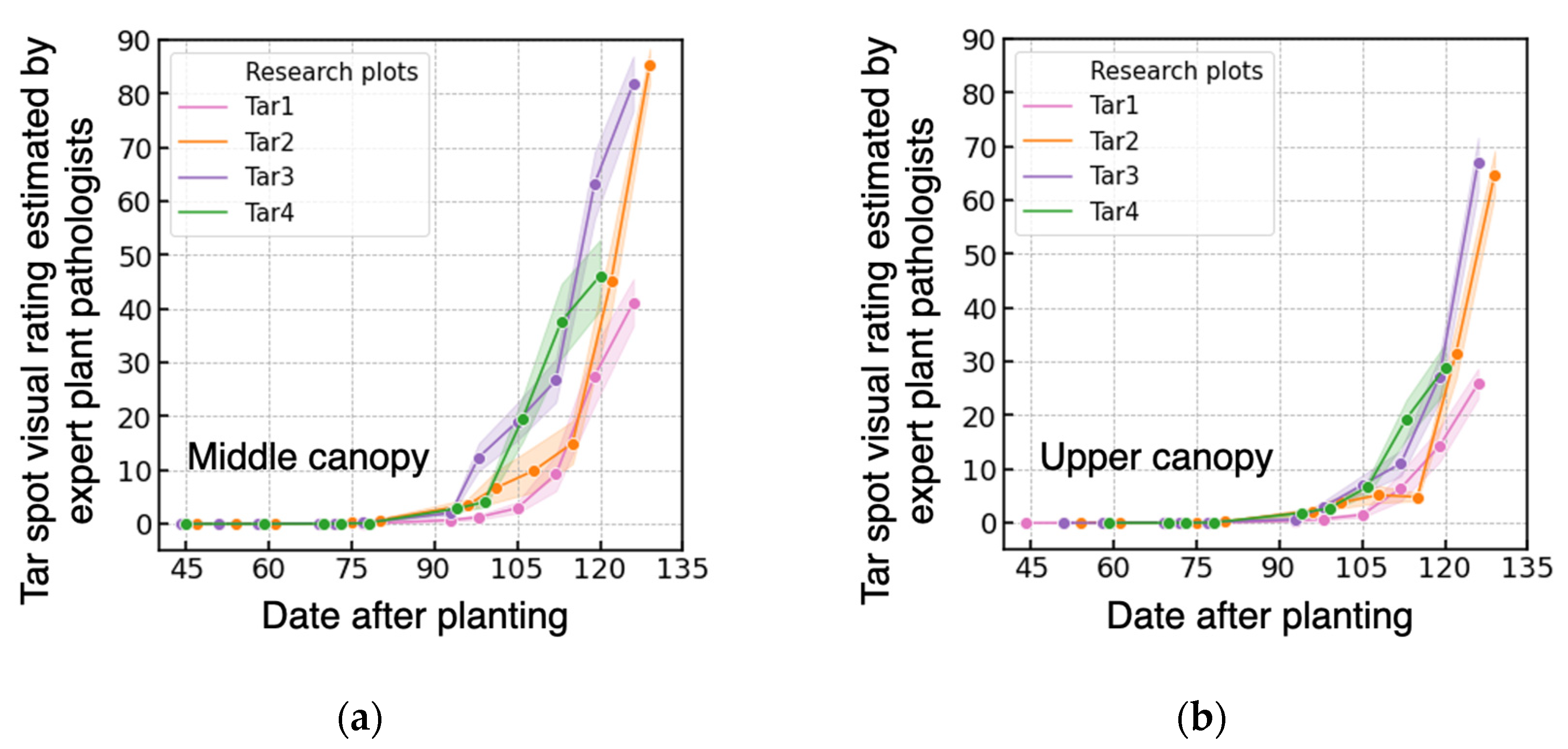
Figure 4.
Tar spot disease rating in (a) middle and (b) upper canopy layers. The average disease severity was shown as dots on the solid lines. The band shaded with color represents the standard deviation of visual rating.
Figure 4.
Tar spot disease rating in (a) middle and (b) upper canopy layers. The average disease severity was shown as dots on the solid lines. The band shaded with color represents the standard deviation of visual rating.
Figure 5.
Preprocessing and plant phenotyping procedure of unmanned aircraft systems (UAS) data. * avg: average, ** stdev: standard deviation.
Figure 5.
Preprocessing and plant phenotyping procedure of unmanned aircraft systems (UAS) data. * avg: average, ** stdev: standard deviation.
Figure 6.
Architecture of multilayer perceptron (MLP) used for UAS-based tar spot measurement. An optimal number of input data and processing nodes in the hidden layer vary according to the spatial resolution of explanatory variables (level 1 grid or level 2 grid) and response variables (visual rating in the middle or upper canopy layer).
Figure 7.
Correlation coefficients between level 1 grid (L1G) unmanned aircraft system (UAS) phenotypes. CCCP: canopy cover derived from the Canopeo algorithm, CV: canopy volume, EXG: average of excessive greenness, MSAVI: modified soil-adjusted vegetation index, NDVI: normalized difference vegetation index, SAVI: soil-adjusted vegetation index, avg: average, mx: maximum, sd: standard deviation.
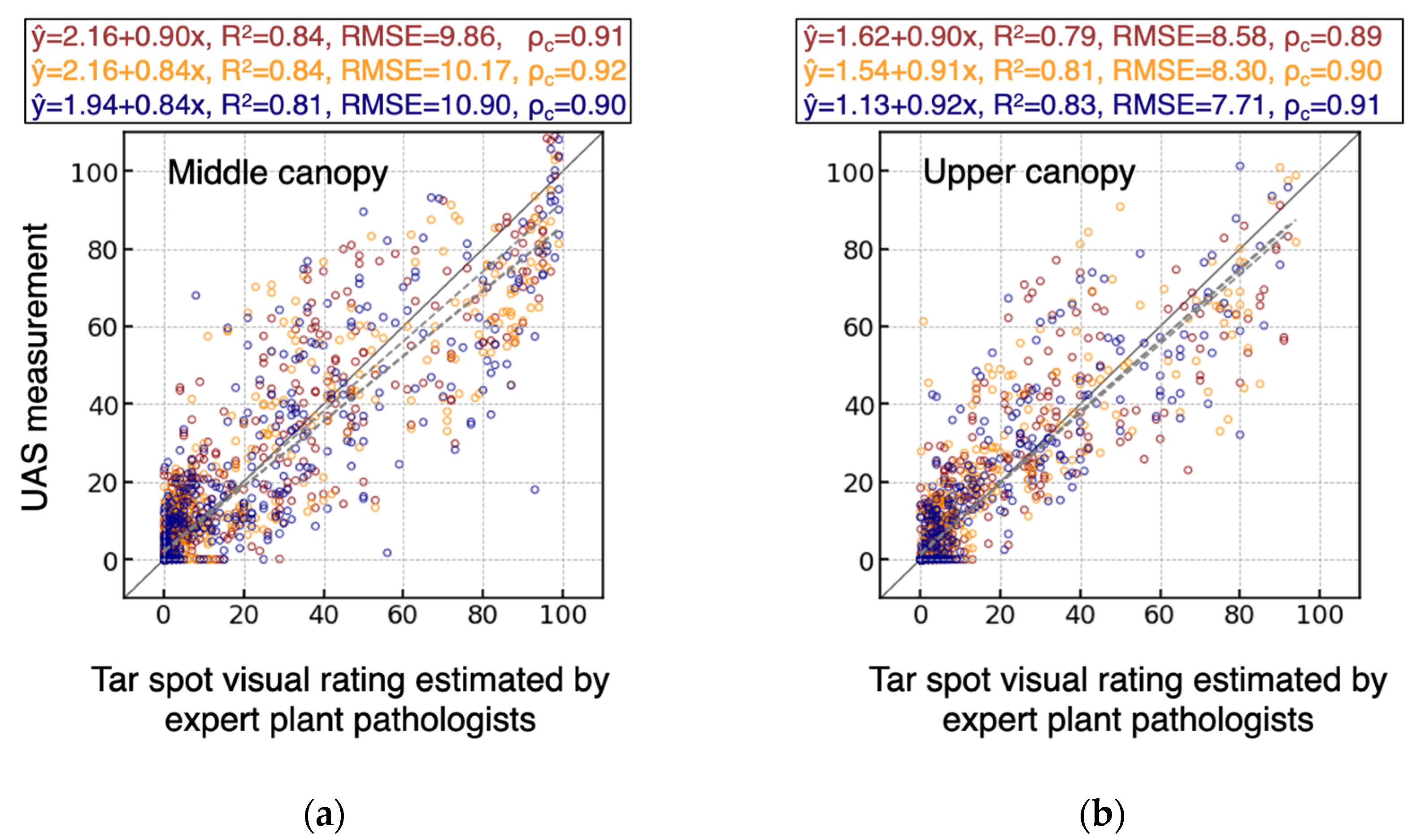
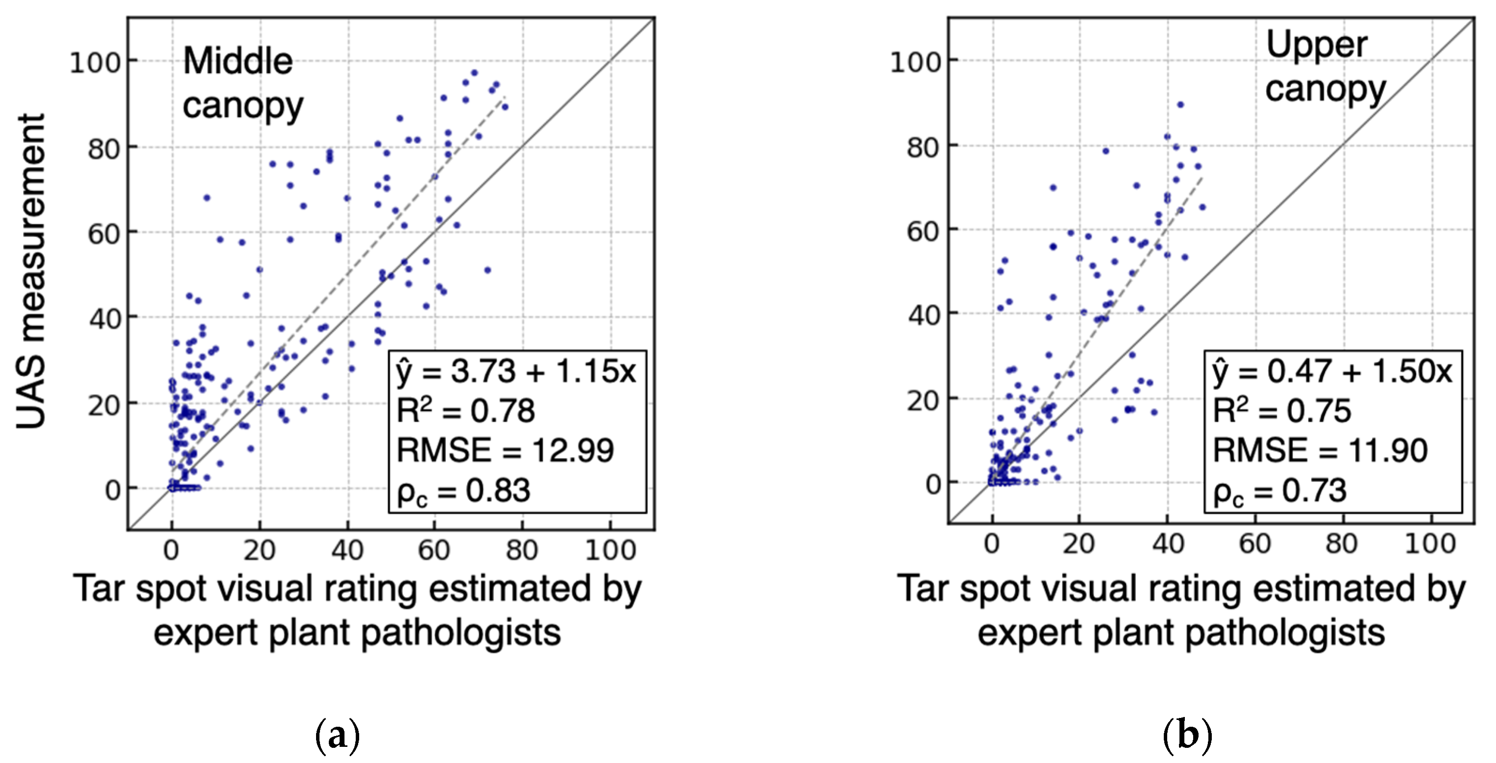
Figure 8.
Tar spot disease rating measured by UAS-based MLP-L1G models at the (a) middle and (b) upper canopy level. The MLP-L1G model was trained with a random split of 3-fold cross-validation of all PPAC data.
Figure 8.
Tar spot disease rating measured by UAS-based MLP-L1G models at the (a) middle and (b) upper canopy level. The MLP-L1G model was trained with a random split of 3-fold cross-validation of all PPAC data.
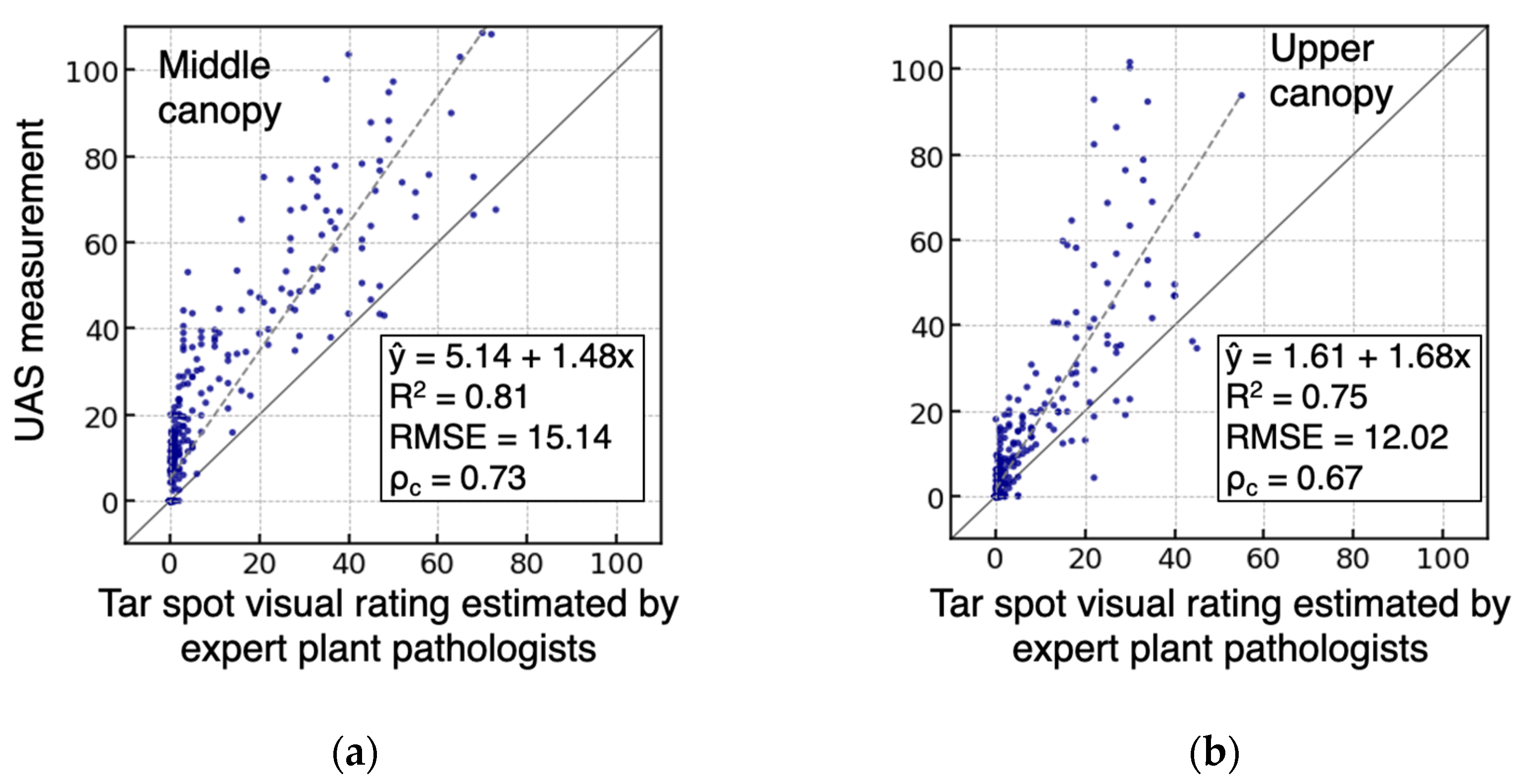
Figure 9.
Tar spot disease rating in Tar1 area measured by UAS-based MLP-L1G model at the (a) middle and (b) upper canopy level. The MLP-L1G model was trained with Tar2, Tar3, and Tar4 data.
Figure 9.
Tar spot disease rating in Tar1 area measured by UAS-based MLP-L1G model at the (a) middle and (b) upper canopy level. The MLP-L1G model was trained with Tar2, Tar3, and Tar4 data.
Figure 10.
Tar spot disease rating in Tar2 area measured by UAS-based MLP-L1G model at the (a) middle and (b) upper canopy level. The MLP-L1G model was trained with Tar1, Tar3, and Tar4 data.
Figure 10.
Tar spot disease rating in Tar2 area measured by UAS-based MLP-L1G model at the (a) middle and (b) upper canopy level. The MLP-L1G model was trained with Tar1, Tar3, and Tar4 data.
Figure 11.
Tar spot disease rating in Tar3 area measured by UAS-based MLP-L1G model at the (a) middle and (b) upper canopy level. The MLP-L1G model was trained with Tar1, Tar2, and Tar4 data.
Figure 11.
Tar spot disease rating in Tar3 area measured by UAS-based MLP-L1G model at the (a) middle and (b) upper canopy level. The MLP-L1G model was trained with Tar1, Tar2, and Tar4 data.
Figure 12.
Tar spot disease rating in Tar4 area measured by UAS-based MLP-L1G model at the (a) middle and (b) upper canopy level. The MLP-L1G model was trained with Tar1, Tar2, and Tar3 data.
Figure 12.
Tar spot disease rating in Tar4 area measured by UAS-based MLP-L1G model at the (a) middle and (b) upper canopy level. The MLP-L1G model was trained with Tar1, Tar2, and Tar3 data.
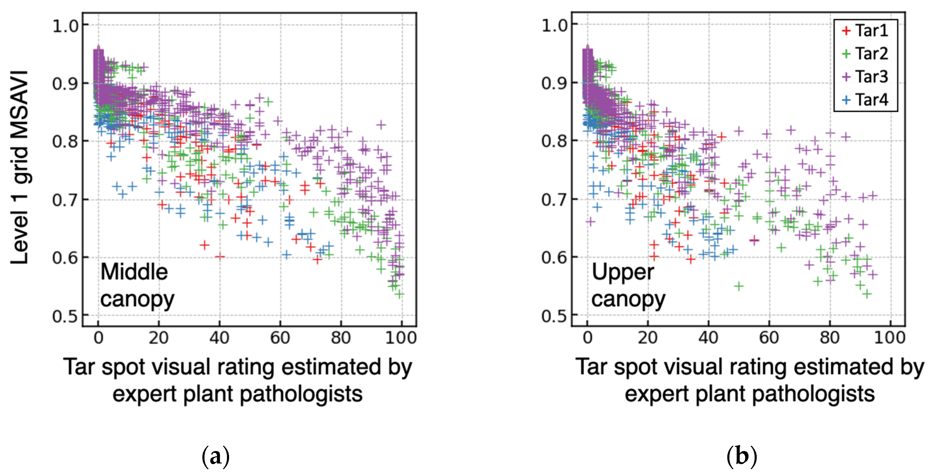
Figure 13.
Tar spot disease rating and level 1 grid (L1G) MSAVI average at the (a) middle and (b) upper canopy level.
Figure 13.
Tar spot disease rating and level 1 grid (L1G) MSAVI average at the (a) middle and (b) upper canopy level.
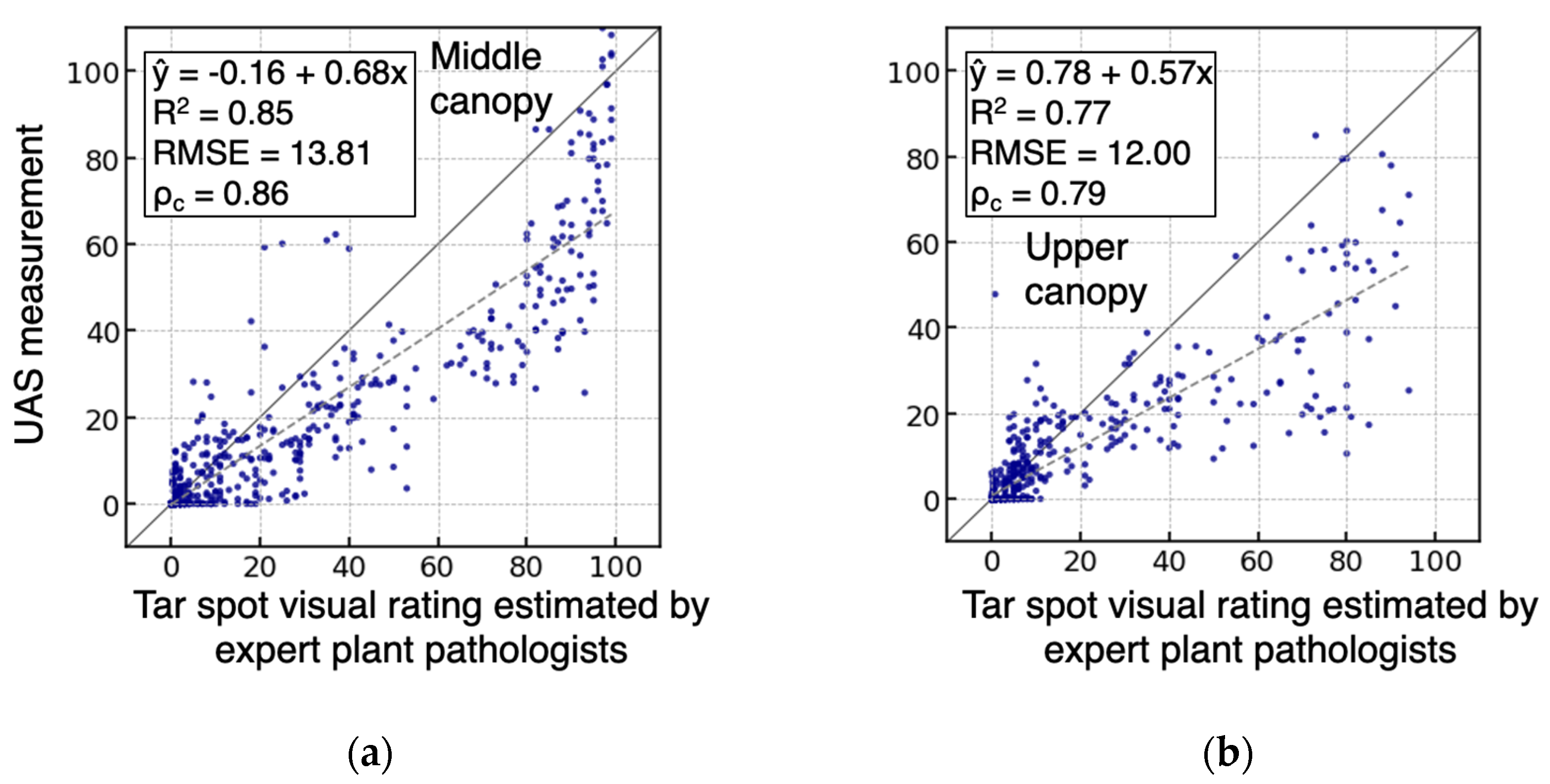
Figure 14.
Tar spot disease rating in Tar4 area measured by UAS-based MLP-L1G model at the (a) middle and (b) upper canopy level. The MLP-L1G model was trained with Tar1 data. A single observer estimated most of the tar spot visual ratings of the Tar1 and Tar4.
Figure 14.
Tar spot disease rating in Tar4 area measured by UAS-based MLP-L1G model at the (a) middle and (b) upper canopy level. The MLP-L1G model was trained with Tar1 data. A single observer estimated most of the tar spot visual ratings of the Tar1 and Tar4.
Table 1.
Description of the experiments at the Pinney Purdue Agricultural Center (PPAC) in Indiana, USA, established in the 2020 cropping cycle.
Table 1.
Description of the experiments at the Pinney Purdue Agricultural Center (PPAC) in Indiana, USA, established in the 2020 cropping cycle.
| Experiment Name | Planting Date | Number of Treatments | Number of Hybrid (s) | Number of Fungicide Treatments | Tillage Type |
|---|
| Trial Tar 1 | 9 June 2020 | 10 | 1 | 9 + 1 (non-treated) | Strip |
| Trial Tar 2 | 6 June 2020 | 12 | 3 | 1 + 1 (non-treated) | Strip, conventional |
| Trial Tar 3 | 9 June 2020 | 18 | 1 | 16 + 2 (non-treated) | Strip |
| Trial Tar 4 | 8 June 2020 | 10 | 1 | 9 + 1 (non-treated) | Strip |
Table 2.
Data acquisition dates of tar spot visual ratings and unmanned aircraft systems (UAS) data. Dates are displayed in MM/DD format for brevity. A: available, N/A: not available.
Table 2.
Data acquisition dates of tar spot visual ratings and unmanned aircraft systems (UAS) data. Dates are displayed in MM/DD format for brevity. A: available, N/A: not available.
| | Tar1 | Tar2 | Tar3 | Tar4 |
|---|
| Visual Rating | UAS Data | Visual Rating | UAS Data | Visual Rating | UAS Data | Visual Rating | UAS Data |
|---|
| 07/13 | A | A | A | A | N/A | A | A | A |
| 07/23 | A | A | A | A | A | A | A | A |
| 07/30 | A | A | A | A | A | A | A | N/A |
| 08/06 | A | A | A | A | A | A | A | A |
| 08/13 | N/A | N/A | A | N/A | N/A | N/A | N/A | N/A |
| 08/17 | A | A | A | A | A | A | A | A |
| 08/20 | A | A | A | A | A | A | A | A |
| 08/25 | A | A | A | A | A | A | A | A |
| 09/03 | A | N/A | A | N/A | A | N/A | A | N/A |
| 09/10 | A | A | A | A | A | A | A | A |
| 09/15 | A | A | A | A | A | A | A | A |
| 09/22 | A | A | A | A | A | A | A | A |
| 09/29 | A | A | A | A | A | A | A | A |
| 10/06 | A | A | A | A | A | A | A | A |
| 10/13 | A | A | A | A | A | A | N/A | N/A |
Table 3.
List of support vector regression (SVR) hyperparameters used in the grid search.
Table 3.
List of support vector regression (SVR) hyperparameters used in the grid search.
| Kernel | ε | C | Kernel Parameters |
|---|
| Linear | 0.05, 0.10, 0.15 | 0.1, 1, 10, 100 | Not applicable |
| Polynomial | 0.05, 0.10, 0.15 | 0.1, 1, 10, 100 | Degree of polynomial = 2, 3 |
| Radial basis function (RBF) | 0.05, 0.10, 0.15 | 0.1, 1, 10, 100 | γ = 10−5, 10−3, 10−1, 10 |
Table 4.
Pearson’s correlation coefficient between visual ratings and level 1 grid (L1G) unmanned aircraft systems (UAS) phenotypes. * avg: average, ** max: maximum, *** stdev: standard deviation.
Table 4.
Pearson’s correlation coefficient between visual ratings and level 1 grid (L1G) unmanned aircraft systems (UAS) phenotypes. * avg: average, ** max: maximum, *** stdev: standard deviation.
| Kernel | Correlation of Level 1 Grid UAS Phenotype and Visual Rating in the |
|---|
| Middle Canopy | Upper Canopy |
|---|
| Canopy cover | −0.72 | −0.67 |
| Canopy volume | +0.09 | −0.03 |
| ExG avg * | −0.41 | −0.36 |
| ExG max ** | −0.41 | −0.37 |
| EXG stdev *** | −0.39 | −0.33 |
| MSAVI avg | −0.87 | −0.83 |
| MSAVI max | −0.82 | −0.81 |
| MSAVI stdev | +0.71 | +0.62 |
| NDVI avg | −0.86 | −0.82 |
| NDVI max | −0.82 | −0.81 |
| NDVI stdev | +0.56 | +0.45 |
| SAVI avg | −0.86 | −0.82 |
| SAVI max | −0.82 | −0.81 |
| SAVI stdev | +0.57 | +0.47 |
Table 5.
Ordinary least square results for middle canopy. R2, adjusted R2, and BIC were 0.78, 0.78, and 1.80 × 10⁴, respectively.
Table 5.
Ordinary least square results for middle canopy. R2, adjusted R2, and BIC were 0.78, 0.78, and 1.80 × 10⁴, respectively.
| | Coefficient | Standard Error | t | p > |t| |
|---|
| Constant | 22.38 | 0.274 | 81.73 | <0.001 |
| Canopy cover | −3.49 | 0.632 | −5.52 | <0.001 |
| Maximum of ExG | 1.84 | 0.354 | 5.12 | <0.001 |
| Average of MSAVI | −44.42 | 0.939 | −47.32 | <0.001 |
| Standard deviation of MSAVI | −8.55 | 0.663 | −12.89 | <0.001 |
Table 6.
Ordinary least square results for the upper canopy. R2, adjusted R2, and BIC were 0.76, 0.76, and 1.53 × 10⁴, respectively.
Table 6.
Ordinary least square results for the upper canopy. R2, adjusted R2, and BIC were 0.76, 0.76, and 1.53 × 10⁴, respectively.
| | Coefficient | Standard Error | t | p > |t| |
|---|
| Constant | 14.00 | 0.211 | 66.23 | <0.001 |
| Canopy cover | −3.02 | 0.506 | −5.97 | <0.001 |
| Maximum of ExG | 2.69 | 0.305 | 8.81 | <0.001 |
| Average of MSAVI | −31.54 | 1.661 | −18.98 | <0.001 |
| Maximum of MSAVI | −3.49 | 1.050 | −3.33 | 0.001 |
| Standard deviation of MSAVI | −9.65 | 0.682 | −14.15 | <0.001 |
Table 7.
Optimal hyperparameters of SVR models.
Table 7.
Optimal hyperparameters of SVR models.
| Canopy Layer | Kernel | ε | C | Kernel Parameters |
|---|
| Middle canopy | RBF | 0.05 | 1 | γ = 0.1 |
| Upper canopy | Polynomial | 0.05 | 0.1 | Degree of polynomial = 3 |
Table 8.
Average and standard deviation of RMSE of unmanned aircraft system (UAS)-based tar spot disease measurement models.
Table 8.
Average and standard deviation of RMSE of unmanned aircraft system (UAS)-based tar spot disease measurement models.
| | Average RMSE of 30 Cross-Validation Trials | Standard Deviation of RMSE of 30 Cross-Validation Trials |
|---|
| | Middle Canopy | Upper Canopy | Middle Canopy | Upper Canopy |
|---|
| OLS with single L1G phenotypes | 12.4 | 10.0 | 0.09 | 0.08 |
| OLS with multiple L1G phenotypes | 11.9 | 9.0 | 0.09 | 0.07 |
| SVR with multiple L1G phenotypes | 11.4 | 10.8 | 0.12 | 0.13 |
| MLP with multiple L1G phenotypes | 10.4 | 7.9 | 0.07 | 0.04 |
| MLP with all L2G phenotypes | 10.4 | 8.2 | 0.06 | 0.06 |


 ,
, 


