Article

The Influence of Solar X-ray Flares on SAR Meteorology: The Determination of the Wet Component of the Tropospheric Phase Delay and Precipitable Water Vapor

by
Aleksandra Nina
1,*,
Jelena Radović
2,
Giovanni Nico
3,4,
Luka Č. Popović
5,6,7,
Milan Radovanović
8,9,
Pier Francesco Biagi
10 and
Dejan Vinković
11
1
Institute of Physics Belgrade, University of Belgrade, 11080 Belgrade, Serbia
2
Department of Atmospheric Physics, Faculty of Mathematics and Physics, Charles University, Ke Karlovu 3, 12116 Prague, Czech Republic
3
Istituto per le Applicazioni del Calcolo (IAC), Consiglio Nazionale delle Ricerche (CNR), 70126 Bari, Italy
4
Department of Cartography and Geoinformatics, Institute of Earth Sciences, Saint Petersburg State University (SPSU), 199034 Saint Petersburg, Russia
5
Astronomical Observatory, 11060 Belgrade, Serbia
6
Department of Astronomy, Faculty of Mathematics, University of Belgrade, 11000 Belgrade, Serbia
7
Faculty of Science, University of Banja Luka, 78000 Banja Luka, Republic of Srpska, Bosnia and Herzegovina
8
Geographical Institute “Jovan Cvijić” SASA, 11000 Belgrade, Serbia
9
Institute of Sports, Tourism and Service, South Ural State University, 454080 Chelyabinsk, Russia
10
Physics Department, Università di Bari, 70125 Bari, Italy
11
Science and Society Synergy Institute, B.J. Jelacica 22, 40000 Čakovec, Croatia
*
Author to whom correspondence should be addressed.
Remote Sens. 2021, 13(13), 2609; https://0-doi-org.brum.beds.ac.uk/10.3390/rs13132609
Submission received: 18 May 2021 / Revised: 19 June 2021 / Accepted: 25 June 2021 / Published: 2 July 2021

Abstract

:
In this work, we study the impact of high-energy radiation induced by solar X-ray flares on the determination of the temporal change in precipitable water vapor ( Δ PWV) as estimated using the synthetic aperture radar (SAR) meteorology technique. As recent research shows, this radiation can significantly affect the ionospheric D-region and induces errors in the estimation of the total electron content (TEC) by the applied models. Consequently, these errors are reflected in the determination of the phase delay and in many different types of measurements and models, including calculations of meteorological parameters based on SAR observations. The goal of this study is to quantify the impact of solar X-ray flares on the estimation of Δ PWV and provide an estimate of errors induced if the vertical total electron content (VTEC) is obtained by single layer models (SLM) or multiple layer models (MLM) (these models do not include ionosphere properties below the altitude of 90 km as input parameters and cannot provide information about local disturbances in the D-region). The performed analysis is based on a known procedure for the determination of the D-region electron density (and, consequently, the vertical total electron content in the D-region (VTEC D )) using ionospheric observations by very low frequency (VLF) radio waves. The main result indicates that if the D-region, perturbed by medium-sized and intense X-ray flares, is not modeled, errors occur in the determination of Δ PWV. This study emphasizes the need for improved MLMs for the estimation of the TEC, including observational data at D-region altitudes during medium-sized and intense X-ray flare events.

Graphical Abstract

1. Introduction

Earth observations based on remote sensing by synthetic aperture radar (SAR) signals can be applied to different types of detection and modeling. In particular, SAR interferometry (InSAR) provides useful information in many applications related to the measurement of displacements and, more recently, in meteorology [1]. SAR meteorology is a recent technique that aims to map precipitable water vapor (PWV) with a high spatial resolution [2,3,4]. The temporal change of PWV between two SAR observations along the same orbit is related to the propagation delay in the atmosphere through a constant that changes slightly based on the properties of the vertical profiles of the atmospheric temperature [5]. Even if the temporal sampling frequency of SAR PWV maps is lower than that of the global navigation satellite system (GNSS) PWV measurements, their higher spatial resolution has a positive impact when assimilated in numerical weather prediction (NWP) models [6,7,8,9]. This can enhance the capability of NWP models to compute the propagation delay in the atmosphere [10] with advantages in other InSAR applications (e.g., the measurement of terrain displacements [11,12,13] and snow water equivalent (SWE) [14,15]).
The basic assumption of SAR meteorology is that there are no terrain displacements between two passes of a SAR sensor over the area of interest, along the same orbit, and that all other phenomena that can affect the propagation delay are negligible (see [6] for more details). In this case, the temporal change in PWV is related to the temporal change in the wet propagation delay between the two passes. However, as a result of the constant exposure to numerous influences, the properties of a medium, which affect signal propagation, are time dependent, and corrections in the calculations are necessary in some cases. The sources of these variations originate in different terrestrial layers and in outer space. In the second case, the ionosphere has the most significant influence on the variability of SAR signal propagation. For this reason, the determination of the total electron content (TEC), a quantity which describes ionospheric influence on electromagnetic signal delay ( P I ), is important. However, insufficient knowledge of perturber characteristics and atmospheric responses make its exact modeling impossible and many approximations must be used because of the various limitations of current remote sensing techniques.
The existing models for the calculation of the vertical total electron content (VTEC) are based on observational data and expressions that give the electron density space dependencies [16,17,18,19,20]. These observational data relate to one (single layer models) or a few (multiple layer models) altitudes which, because of the large electron density, primarily lie in the upper ionosphere. For this reason, these models cannot “see” local ionospheric disturbances at the D-region altitudes (50–90 km) and, consequently, do not provide a good enough approximation of P I for satellite signals in periods when intense disturbances dominate the lower ionosphere. This problem is reported for the first time in [21] a study of satellite signal delay in the ionospheric D-region disturbed by a solar X-ray flare.
The increased X-radiation emitted during a solar X-ray flare primarily affects the ionospheric D-region, in which the electron density and corresponding part of the vertical total electron content ( VTEC D ) can increase by more than two orders of magnitude with respect to their values under quiet conditions [22,23,24]. Although the electron density in the D-region is lower than in the F-region, whose contribution is dominant in the TEC, the study presented in [21] indicates that solar X-ray flare-induced disturbances within the D-region can be important in calculating and modeling satellite signal delays. As a consequence, the results obtained in this paper indicate the need for further analyses concerning the influence of solar X-rays on the application of observations by GNSS and SAR signals.
In this paper, we focus on SAR meteorology and the estimations of Δ ϕ wet and differences in the precipitable water vapor (ΔPWV) during periods in which the master and slave images are recorded by a SAR satellite. We present a procedure for modeling the correction factor that should be included in the determination of Δ ϕ wet ( B D ), and the correction factor that should be included in the determination of ΔPWV ( C D ) if the influence of a solar X-ray flare is present in one of the two considered time periods. The study consists of two analyses: first, we consider one particular X-ray flare and calculate B D and C D dependencies on the X-ray flux during this event; second, we determine B D and C D for maximum X-ray flux for solar X-ray flares using ionospheric parameters derived in [24] and based on the statistical analysis presented in [25]. In both cases, four frequencies are considered: 1.2 GHz and 5.4 GHz, which are the operating frequencies of radar systems on board the advanced land observing satellite-2 (ALOS-2) and Sentinel-1 satellites, respectively; 0.43 GHz, which is the frequency of the radar system on board the planned BIOMASS mission; and 3.4 GHz, which is one of the two frequencies that will be used by the radar system on board the planned joint mission involving National Aeronautics and Space Administration (NASA) and Indian Space Research Organisation (ISRO), known as the NASA-ISRO Synthetic Aperture Radar (NISAR) (the other frequency is 1.2 GHz, as is the case for ALOS-2).
The paper is organized as follows. After describing the geostationary operational environmental satellite (GOES),very low/low frequency (VLF/LF), and SAR measurements in Section 2, we present our proposed methodology in Section 3. The results of the presented model when apply to the particular event and ionospheric conditions at the X-ray flux maximum, during class-C and -M solar X-ray flares, are shown in Section 4. The conclusions of this study are given in Section 5.

2. Observations

The procedure presented in this study is based on data collected by the GOES satellite measuring the X-ray flux and by VLF/LF receivers using radio waves to sound the lower ionosphere. In addition, the proposed methodology needs the working frequency of SAR systems as an input parameter.

2.1. GOES Satellite Measurements

The measurements of solar X-ray flux provided by the GOES satellite allow for the detection of solar X-ray flares and the analyses of the energy properties of the ionized radiation perturbing the ionospheric D-region. These measurements are captured by two detectors in the energy channels A and B, corresponding to the wavelength domains 0.05 nm–0.4 nm and 0.1 nm–0.8 nm, respectively.
Considering that the temporal evolutions of fluxes recorded by these detectors are different, it is first necessary to pay attention to the determination of the X-ray flux values Φ relevant to this study. The contribution of X-ray photons with wavelength λ in total ionization in the terrestrial ionosphere depends on the altitude (e.g., see [26]). However, the comparison of the temporal evolution of the electron density at a given altitude, and fluxes recorded by the GOES energy channels A and B, presented in [27], shows that the recorded flux in channel A is more relevant for the lower D-region, and that the recorded flux in GOES channel B better describes the influence of an X-ray flare in the upper part of this ionospheric layer. Considering that the electron density increases with altitude, i.e., the upper D-region provides the dominant contribution to the VTEC D , we assume that Φ is the flux recorded by the GOES channel B. The data recorded through this channel are also used in many previous studies of reactions in the low ionosphere [28,29,30].
Datasets of the X-ray fluxes recorded by the GOES satellites with samples of approximately 2 s are available on the NOAA’s National Centers for Environmental Information website (http://satdat.ngdc.noaa.gov/sem/goes/data, accessed on 18 May 2021). Values corresponding to the X-ray flare that occurred on 6 January 2015 are shown in the upper left panel of Figure 1.

2.2. VLF/LF Measurements

The VLF/LF radio waves propagate in the Earth–ionosphere waveguide, the upper border of which lies in the analyzed atmospheric layer. Applications of this measurement technique in lower ionospheric observations and research are based on the fact that changes in the ionospheric electron density have the most significant influence on variations in the signal amplitude and phase recorded by a VLF/LF receiver. This makes the VLF/LF radio technique a useful tool for remote sensing in the ionosphere D-region. For this reason, we are able to study the influences of many astrophysical and terrestrial phenomena in this layer, such as ionospheric disturbances induced by gamma ray bursts [31,32], solar X-ray flares [33,34,35,36], tropical cyclones [37,38,39], and lightning [40,41,42]. In addition to independent receivers, there are several networks that are very important for the spatial analyses of local perturbations, such as those induced by earthquakes (the International Network for Frontier Research on Earthquake Precursors (INFREP) [43]) and lightning (the World Wide Lightning Location Network (WWLLN) [44]).
Practical applications of D-region disturbance modeling based on data recorded using this type of observational equipment are very important during solar X-ray flares. In certain cases, intense disturbances can last several hours and the electron density can increase by more than two orders of magnitude [22,23]. For this reason, we chose to analyze periods when this phenomenon affects the Earth’s atmosphere.
Firstly, in relation to the analysis of a particular event, we consider the amplitude (ΔA) and phase (ΔP) changes with respect to quiet conditions for signal emitted by the DHO transmitter in Germany and recorded by the atmospheric weather electromagnetic system for observation modeling and education (AWESOME) receiver [45] located in Belgrade, Serbia. The temporal evolution of the signal characteristics and their dependencies on X-ray flux during the considered flare, which occurred on 6 January 2015, are presented in Figure 1. As one can see, both dependencies on X-ray flux have hysteresis-like shapes; these are the result of the ionospheric plasma properties response to the increase in the photo-ionization rate, which itself depends on electron loss processes.

2.3. SAR Characteristics

Frequency and polarization are the two main characteristics of the SAR signal, useful when modeling their propagation in the ionosphere D-region. Because this paper is focused on the mitigation of ionosphere artifacts in SAR meteorology applications, we only consider the frequency of the SAR signal. Generally, propagation delay maps are obtained by interferometrically processing two SAR images to derive the interferometric phase [10]:
Δ φ atm = 4 π λ R atm = 10 6 4 π λ 0 H sat Δ N d h ,
where Δ R atm and Δ φ atm are the temporal changes of the range and interferometric phase delays due to propagation through the whole atmosphere at the acquisition times of the master and slave SAR images, respectively, λ is the radar wavelength, H sat is the altitude of satellite, and Δ N is the temporal change in refractivity along the propagation path of the radar signal. The relationship between the interferometric phase and propagation delay solely depends on the signal frequency. If fully polarized SAR images are used, other effects can be observed and quantified, such as the Faraday rotation effect. However, this effect does not affect the propagation delay and it is not taken into consideration as a possible artifact in SAR meteorology applications. The mapping of temporal change in PWV requires the estimation of the propagation delay caused by the wet component of atmospheric refractivity and the vertical profile of temperature [5]:
Δ PWV = Π Z W D ,
where Π is a function of the mean temperature along a vertical profile and Z W D is the zenith wet delay obtained by projecting the wet component of the propagation delay in a vertical direction [5]. The estimation of the wet delay is performed by modeling and removing the temporal change of the other components of propagation delay (mainly the hydrostatic components, but also others related to the ionosphere) from the Δ R a t m . The impact of uncertainty on the estimation of the propagation delay is studied in [10]. In this paper, we focus on the C-, L-, and P-bands. The C-band is of key importance for SAR meteorology applications as a result the free access to Sentinel-1 SAR data. The L-band is more applicable in atmospheric studies, because it is directly comparable to GNSS measurements, which work in the L-band. However, thus far, the L-band ALOS-2 mission does not provide data with the same temporal revisiting time as Sentinel-1. The new satellites for observation and communications (SAOCOM) mission of Argentina’s space agency [46] and NISAR, the joint mission between NASA and ISRO, [47], will increase the availability of L-band SAR data. ALOS-2 and SAOCOM work in the following frequencies: f = 1.200 GHz and f = 1.275 GHz, respectively. NISAR will carry both an L-band ( λ = 24 cm) and S-band: ( λ = 9 cm) radar. In this work, we also consider the P-frequency band that will be used by the BIOMASS mission planned to be launched by the European Space Agency in 2022 [48]. The frequencies and wavelengths of these satellites are summarized in Table 1.

3. Modeling Δ PWV Corrections Resulting from the Influence of a Solar X-ray Flare

In this section, we describe a methodology for modeling the influence of the X-ray flare-perturbed D-region on the measurements of Δ PWV currently obtained by InSAR meteorology and provide a means to estimate the necessary correction resulting from X-ray flare effects. Modeling of the solar X-ray-perturbed D-region influence on Δ PWV can be divided into two steps: 1. calculations of the electron density ( N e ) and, consequently, VTEC D ; 2. the determination of the corresponding correction factors B D and C D , in calculations of Δ ϕ wet and ΔPWV, respectively. A description of these steps is given in the following, and a schematic view of this methodology is presented in Figure 2.

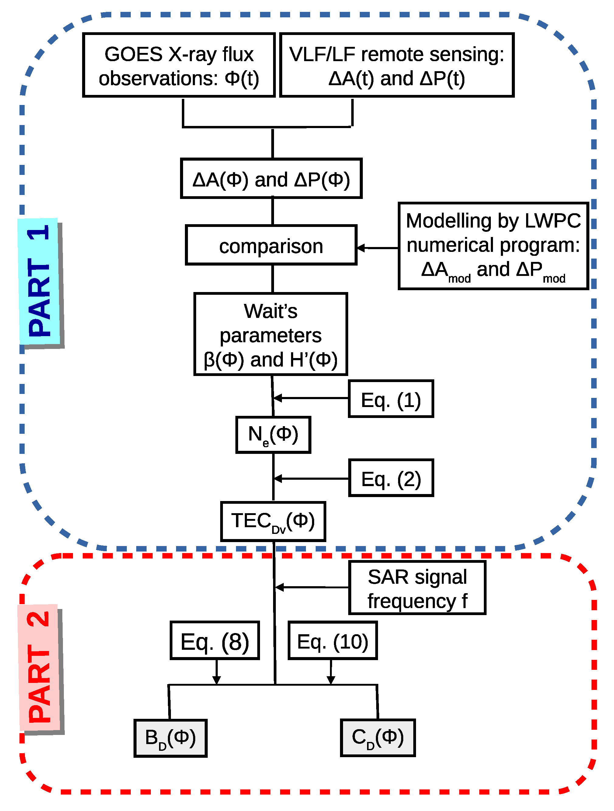
3.1. Determination of VTEC D

The determination of VTEC D during a solar X-ray flare is explained in [21] in detail. In this study, we apply very similar procedures, which substitutes dependencies on the time evolution to dependencies on the X-ray flux. It consists of the observation and modeling, and its main steps are as follows:
  • The determination of the period when the considered X-ray flare affected the terrestrial atmosphere from data collected by a GOES satellite;
  • The determination of the considered time period from the temporal evolution of the DHO signal amplitude and phase recorded by the AWESOME VLF receiver in Belgrade. These variations are used because the ionosphere perturbations last longer than the increase in the X-radiation;
  • The extraction of time series data recorded by the GOES energy channel B ( Φ ( t ) ), and the VLF receiver ( Δ A ( t ) , and Δ P ( t ) ) in the considered time interval;
  • The determination of Δ A ( Φ ) and Δ P ( Φ ) . As presented in Figure 2, these relationships are obtained in comparison with the recorded datasets (given in time);
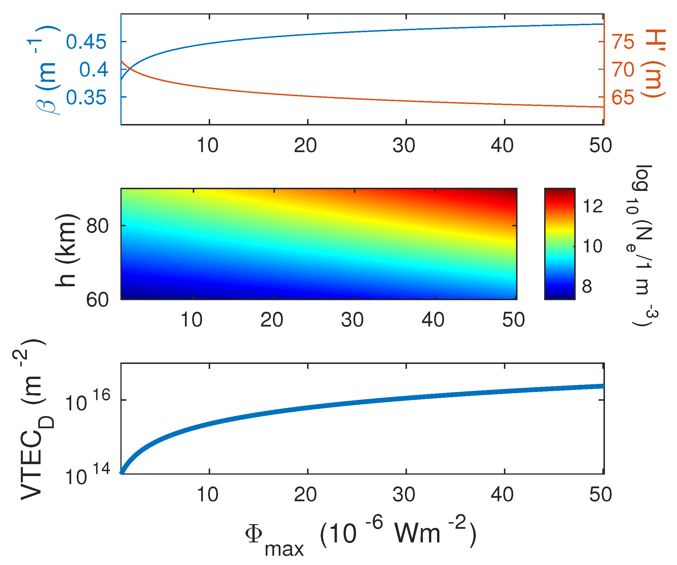
  • The determination of N e ( Φ , h ) in the D-region altitude domain. We use the Wait model of the ionosphere [49], which is based on two ionospheric parameters: the “sharpness” ( β ) which describes the electron density vertical gradient, and signal reflection height ( H ) which shows at what altitude the VLF or LF signal is reflected from the ionosphere. These parameters are determined by comparing the recorded values ΔA and ΔP with corresponding values modeled using the long-wave propagation capability (LWPC) numerical program for the simulation of the signal propagation in the Earth–ionosphere waveguide developed by the Space and Naval Warfare Systems Center, San Diego, USA [50]. This procedure is explained in [51] and is applied in several previous studies [22,52,53]. The initial values of Wait’s parameters β and H in quiet conditions before the influence of the considered flare are determined using the Quiet Ionospheric D-Region (QIonDR) model [54]. Knowledge of the time evolution of Wait’s parameters allows the electron density time-altitude distribution to be calculated using equation [55]:
    N e ( t , h ) = 1.43 × 10 13 e β ( t ) H ( t ) e ( β ( t ) 0.15 ) h ,
    which is used in numerous previous papers [56,57,58,59]. Here, N e , β , and H and the considered D-region altitude h are given in m 3 , km 1 and km, respectively;
  • The determination of the vertical total electron content time evolution VTEC D ( t ) within the D-region altitude domain h D (60–90 km) using Equation [24]:
    VTEC D ( Φ ) = h D N e ( Φ , h ) d h .
The obtained values of VTEC D are input values in the second part of the presented procedure.

3.2. Determination of B D and C D

The determination of B D and C D depends on both the D-region and SAR signal properties. In this study, we present a procedure for its estimation. Before describing this method, it is important to note that a solar X-ray flare significantly influences the determination of Δ ϕ wet and ΔPWV during one or both periods relevant for master and slave SAR images. However, the second case is very rare and, for this reason, we focus our attention on the first.
Considering that Δ ϕ wet is one of the components of the phase delay Δ ϕ , it can be calculated from Equation [9]:
Δ ϕ = Δ ϕ top + Δ ϕ wet + Δ ϕ hyd + Δ ϕ ion ,
where Δ ϕ top , Δ ϕ hyd , and Δ ϕ ion relate to changes in the terrain morphology, the hydrostatic component of tropospheric delay, and ionospheric delay during the two considered periods, respectively. Because a solar X-ray flare has no influence on terrain morphology or tropospheric parameters, Equation (5) demonstrates that parameter B D represents the difference in Δ ϕ wet , in cases in which the influence of X radiation is and is not considered (relevant values in the following are indicated by “*” and “o” in the superscript, respectively) [16]:
B D = Δ ϕ ion o Δ ϕ ion * .
The phase delay in the ionosphere due VTEC is given by the following [16]:
ϕ ion = 4 π λ K f 2 cos ( ϑ look ) VTEC ,
which gives their differences: Δ ϕ ion o = 4 π λ K f 2 cos ( ϑ look ) Δ VTEC and Δ ϕ ion m / s * = 4 π λ K f 2 cos ( ϑ look ) ( Δ VTEC VTEC D ) . Here, K = 40.28 m 3 /s 2 , VTEC is the difference in the VTEC between the slave and master acquisition times, where t s l a v e > t m a s t e r , and VTEC D is the additional VTEC variation due to an anomaly in the D-region. This quantity is added to or subtracted from Δ VTEC if this X-ray flare occurs at the slave or master acquisition time, respectively. Cases in which a flare affects the atmosphere at the master and slave acquisition times are indicated by subscripts “m” and “s”, respectively. The combination of these relationships with Equations (6) and (7) gives the equation for B D m / s in the following form:
B D m / s = ± 4 π λ K f 2 cos ( ϑ look ) VTEC D ,
where one can see that B D is proportional to VTEC D and cos 1 ( ϑ look ) . Δ PWV can be determined from the unwrapped phase Δ ϕ , which is obtained by filtering and unwrapping the wet component of the tropospheric delay δ ϕ [5]:
Δ PWV = λ 4 π cos ( ϑ look ) ρ ξ δ ϕ ,
where λ is the radar wavelength, ϑ look is the look angles along the swath, and ρ and ξ are constants, whose values are 1000 kg·m 3 (the density of water) and 6.4, respectively.
Assuming δ ϕ o δ ϕ * B D m / s , Equations (8) and (9) give
C D m / s = Δ PWV o Δ PWV * = ± K f 2 ρ ξ VTEC D .
This equation shows that correction factor C D is proportional to VTEC D and to f 2 . In other words, the influence of an X-ray flare on Δ PWV increases with its intensity, and has a larger effect on SAR signals with a lower frequency. In addition, it is important to note that the presented procedure demonstrates that the look angles along the swath ϑ look do not affect C D . This fact is a consequence of the linear dependence of Δ ϕ wet on cos ( ϑ look ) , and the reverse relationship between VTEC D and cos ( ϑ look ) .
As one can see from Equations (8) and (10), absolute values of both correction factors are the same in cases when a solar X-ray flare occurs at the master and slave acquisition time. For this reason, we further analyze B D and C D , e.g., the absolute values of quantities B D m / s and C D m / s , respectively.

4. Results and Discussion

The presented methodology for the estimation of the correction factors B D and C D is applied to two analyses relating to: 1. the dependencies of B D and C D on the X-ray flux ( Φ ) during one solar X-ray flare, and 2. the dependencies of B D and C D on the maximum X-ray flux ( Φ max ) for flares of classes C and M.

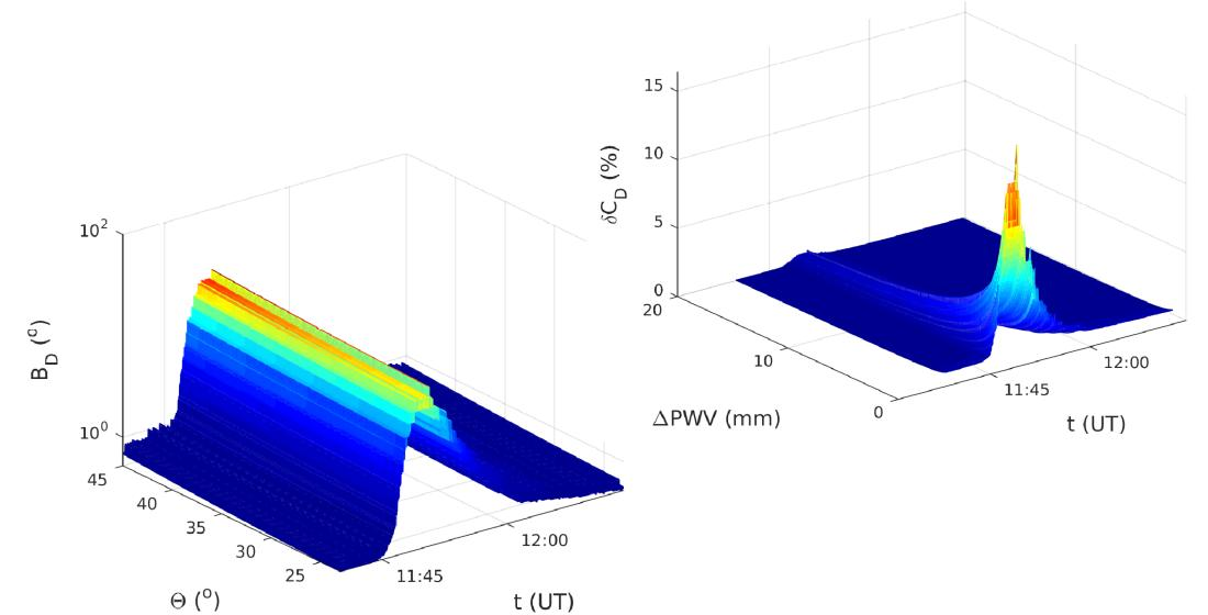
4.1. Particular X-ray Flare Event

As it can be seen in previous studies (see, for example, [58]), variations in the D-region electron density during solar X-ray flares have very similar characteristics, which allows us to study the properties of the dependences B D ( Φ ) and C D ( Φ ) in analysis of one event. Here, we present a detailed analysis for period during the class-C9.9 X-ray flare, which occurred on 6 January 2015. In addition, we show the results obtained for two more flares of classes C8.8 and C6.1, which occurred on 5 May 2010 and 8 January 2014, respectively (see Supplementary Material).
According the methodology shown in Figure 2, the comparison of the observed amplitude ΔA and phase ΔP changes (see Figure 1), and the corresponding values obtained by modeling the considered VLF signal propagation using the LWPC numerical model gives us Wait’s parameters β and H for each value of the X-ray flux Φ (upper panel of Figure 3). As one can see, β first increases with Φ . Although Φ decreases after Φ max , β continues to increase for some time and reaches a maximum value for Φ 8.7 × 10 6 Wm 2 , after which it begins to decrease. The changes in H run counter to those of the first parameter. In both cases, the values are not equal for the same Φ before and after the X-ray flux maximum and these dependencies have hysteresis-like shapes. During the period in which Φ increases, the changes in Wait’s parameters are slower for the smallest values of Φ . The properties are better visible in the dependencies of the electron density N e on Φ and altitude h before (the second panel) and after (the third panel) the X-ray flux maximum, as calculated by Equation (3). These properties are in agreement with the analysis given in [27], which describes them in detail. Here, we indicate that they can be explained according to complex processes in the ionospheric plasma, i.e., electron density changes depend on both ionization and electron loss processes, which induce an increase and decrease in N e . The rate of the first type of processes (G) is larger than the second (L) during the increase in Φ and some time after its maximum value. In this period, N e increases. After that, G < L and N e have the tendency to reach their initial values. Considering that L depends on the ionospheric state, its values are not the same for the same Φ before and after Φ max , which, together with the changes in the spectrum of the incoming X radiation in the considered area, explains the corresponding differences in N e ’s (and Wait’s parameters’) dependencies on Φ .
Finally, VTEC D ’s dependence on Φ is shown in the bottom panel of Figure 2. Its shape is the same as β , while the maximum difference for the same Φ is about one order of magnitude.
The application of Equations (8) and (10) to the obtained values of VTEC D , and signal frequencies f 1 = 0.43 GHz, f 2 = 1.2 GHz, f 3 = 3.2 GHz, and f 4 = 5.4 GHz, gives dependencies B D ( Θ , Φ ) and C D ( Φ ) , respectively.
To better visualize the signal frequency influence on B D ( Θ , Φ ) , we use the same color map scale for all four graphs in Figure 4, which present the results for the BIOMASS (upper left graph), ALOS-2 (upper right graph), NISAR (bottom left graph), and Sentinel-1 (bottom right graph) satellites. The upper panels for each satellite correspond to the period before Φ max , while values obtained for the period after Φ max are presented in the bottom panels. As one can see, B D varies more than one order of magnitude for all satellites and all angles during the considered flare. Its values strongly depend on the signal frequency (∼ f 2 ) and differ more than one order of magnitude for the satellites with the lowest (BIOMASS) and the largest (Sentinel-1) frequency when the other parameters are the same. The maximal values of B D are 25.36 o , 18.86 o , 3.55 o , and 2.06 o for the BIOMASS, ALOS-2, NISAR, and Sentinel-1 satellites, respectively. According to Equation (8), the maximal values of B D correspond to Φ measured at the peak of VTEC D . Variations with Θ are weak and they are more pronounced for the ALOS-2 satellite, in which the operating angle domain is the widest and reaches the lowest values (as B D cos 1 ( Θ ) , these variations increase with Θ , which is clearly visible in the relevant graph). The maxima of B D are for the largest Θ , which can be seen from Equation (8) and from the fact that Θ has values lower than 90 o .
Dependencies of C D on Φ are shown in Figure 5. Their quantitative description (for one frequency) is the same as that for β and VTEC D . As in the case of B D , this correction factor is proportional to VTEC D and f 2 (see Equation (10)). For all frequencies, C D reaches values that are more than one order of magnitude larger in the moment of the most intense D-region disturbance. Its maxima are 0.16 mm, 0.02 mm, 0.003 mm, and 0.001 mm for the BIOMASS, ALOS-2, NISAR, and Sentinel-1 satellites, respectively. To estimate the importance of these values, which represent errors in the modeling of Δ PWV due to the influence of the increased X-radiation during a solar X-ray flare, we calculated their ratio with absolute values of Δ PWV obtained in [60]. The domain of Δ PWV is from about −22 mm to 8 mm. Although they include the results of calculations with absolute values lower than 1 mm, we do not present them in Figure 6. This is because despite providing a large considered ratio δ C D = C D | Δ PWV | × 100 % , they are not as important for practical applications. As it can be seen in Figure 6, the obtained δ C D increases with VTEC D and reaches 15.6%, 2.0%, 0.3%, and 0.1% for the BIOMASS, ALOS-2, NISAR, and Sentinel-1 satellites, respectively. Here, we can see that the signal frequency is important in the determination of the considered error, which, in the case of this flare of class C, is only larger than 10% for the BIOMASS satellite.
As one can see in Supplementary Materials, very similar graphs are obtained for the other two analyzed X-ray flares. The plots are quite similar like those described in the previous text, and B D , C D , and δ C D reaches similar values like in the case of the first analyzed flare.

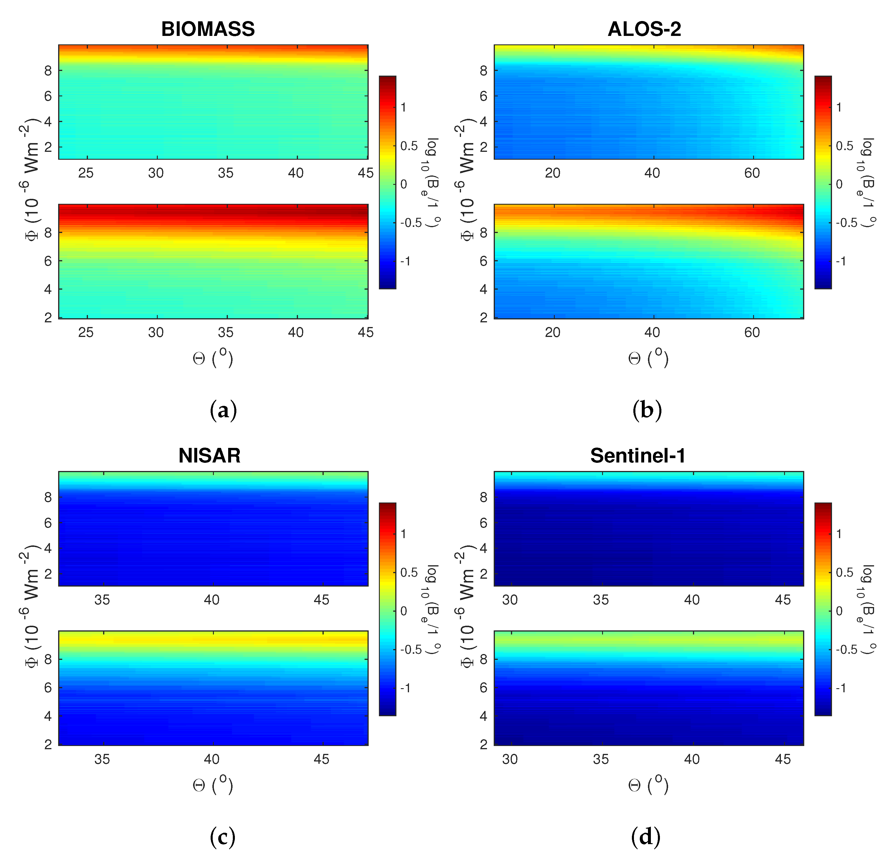
4.2. Maximum X Radiation Flux

To analyze the influence of the X-ray flare class on the determination of Δ ϕ wet and Δ PWV in SAR meteorology, we study the dependence of B D and C D on the radiation flux maximum Φ max . In this case, we calculate the VTEC D using expressions for Wait’s parameters derived in [24] by processing data based on the observation and statistical study in [21,25]. Considering that the application of Equation (3) better fits with the values obtained by other models for flares of classes C and M than for flares of class X, we consider the dependency for Φ max 5 × 10 5 Wm 2 . All calculations are performed using the same equations as in the previous corresponding analyses.
The dependences of Wait’s parameters, the electron density at D-region heights, and the total electron content on Φ max are shown in Figure 7. As one can see, all quantities increase with Φ max except H which has the opposite tendency. The maximum calculated VTEC D ( 2.4 × 10 16 m 3 ) is more than five times that of the flare analyzed in the first part of this study ( 4.6 × 10 15 m 3 ), which again provides larger errors in the estimation of Δ ϕ wet and Δ PWV .
The influences of f, Θ , and Φ max on B D are illustrated in Figure 8. According to Equation (8), B D is proportional to f 2 and cos 1 ( Θ ) , as in the case of one event. However, in this analysis, B D monotonically increases with Φ max because of the increase in VTEC D with this radiation flux. For the considered domains, the most important variations are recorded for different Φ max (of more than two orders of magnitude). The influence of the chosen frequency is also important (they can provide variations in B D for more than one order of magnitude), while the lowest significance has Θ , which, as in the first case, is the most pronounced for the ALOS-2 satellite. The maximum obtained values are 132.8 ° , 98.8 ° , 18.6 ° , and 10.8 ° for the BIOMASS, ALOS-2, NISAR, and Sentinel-1 satellites, respectively. This is more than five times larger than in the case of the flare considered in the first part of this study, which indicates that the intensity of the considered X-ray flare has a significant influence.
Increases in C D with Φ max are shown in Figure 9. As is the case for the analysis of one flare, the considered correction factor decreases with signal frequency and, for M5 X-ray flares, reaches values of 0.81 mm, 0.10 mm, 0.015 mm, and 0.0052 mm for the BIOMASS, ALOS-2, NISAR, and Sentinel-1 satellites, respectively. The maximum obtained values reach 81.7%, 10.5%, 1.5%, and 0.5% of those for Δ PWV presented in [60] for the considered satellites, respectively.
The tendencies of the obtained dependencies B D ( Φ max ) and C D ( Φ max ) indicate that more intense flares (firstly, class X flares) can induce non-negligible errors in the determination of ϕ wet and Δ PWV for the BIOMASS and ALOS-2 satellites (Figure 10).

5. Conclusions

In this paper, we study how neglecting the D-region electron density temporal variations in the determination of the total electron content by single and multiple layer models affects results in synthetic aperture radar meteorology when this ionospheric region is significantly disturbed. We present an analysis of the correction factors that should be included in the determination of differences in the wet component of tropospheric phase delay and precipitable water vapor obtained by synthetic aperture radar meteorology during a solar X-ray flare event. We study the dependence of these correction factors on X-ray flux during an X-ray flare event, and C- and M-class flares at the time of their maximum radiation intensity. The obtained results show the following:
  • The correction factors for the same radiation flux are larger in the period after than in the period before the radiation maximum;
  • During a solar X-ray flare event, the maxima of the considered correction factors pertain to the radiation flux that is lower than its maximum value and that occurred after the radiation maximum. For the X-ray flare that occurred on 6 January 2015, the correction factor that should be included in the determination of differences in the wet component of tropospheric phase delay reaches 25.36 ° , while the correction factor that should be included in the determination of temporal changes in the precipitable water vapor can reach 0.16 mm (this value can be more than 15% of the values for precipitable water vapor changes given in [60]);
  • The correction factors increase with the maximum X-ray flux. For the considered fluxes, the correction factor that should be included in the determination of differences in the wet component of tropospheric phase delay can reach more than 130 ° while the correction factor that should be included in the determination of changes in the precipitable water vapor can reach 0.8 mm, which can be more than 80% of the values for precipitable water vapor changes given in [60];
  • The correction factors are inversely proportional to the square of the frequency. The differences for the considered maximal and minimal frequencies are more than two orders of magnitude for the correction factor in the determination of changes in the wet component of tropospheric phase delay, and more than one order of magnitude for the correction factor in the determination of changes in the precipitable water vapor, in the case of the same X-ray intensity. The changes are also pronounced as regards the variation in the X-ray flux, while changes in B D with the signal angle are the weakest (they are the largest in the case of the advanced land observing satellite-2 due to the wider operating angle range and the largest angles).
To conclude, this is the first study to analyze the errors induced by intense ionospheric D-region disturbances (in this study, induced by a solar X-ray flare) in the practical application of synthetic aperture radar signals. We found that the inclusion of the D-region altitude in the calculation of the total electron content, which is used to determine changes in the wet component of tropospheric phase delay and precipitable water vapor using synthetic aperture radar meteorology, is necessary during larger solar X-ray flare events. It has a larger influence on lower frequency signals and is most important for the BIOMASS satellite.

Supplementary Materials

The following are available online at https://0-www-mdpi-com.brum.beds.ac.uk/article/10.3390/rs13132609/s1, Table S1: The maximal values of the correction factor in the determination of changes in the wet component of tropospheric phase delay (BDmax), correction factor in the determination of changes in the precipitable water vapor (CDmax), and ratio (in percent) of the correction factor in the determination of changes in the precipitable water vapor and absolute values of changes in the precipitable water vapor presented in [1] (dCDmax) during a solar X-ray flare, which occurred on 5 May 2010 for the BIOMASS, ALOS-2, NISAR, and Sentinel-1 satellites, Table S2: The maximal values of the correction factor in the determination of changes in the wet component of tropospheric phase delay (BDmax), correction factor in the determination of changes in the precipitable water vapor (CDmax), and ratio (in percent) of the correction factor in the determination of changes in the precipitable water vapor and absolute values of changes in the precipitable water vapor presented in [1] (dCDmax) during a solar X-ray flare, which occurred on 8 January 2014 for the BIOMASS, ALOS-2, NISAR, and Sentinel-1 satellites.

Author Contributions

Conceptualization, A.N.; methodology, A.N.; software, A.N.; validation, G.N., L.Č.P., P.F.B. and D.V.; formal analysis, A.N., J.R., G.N. and L.Č.P.; investigation, A.N.; resources, A.N.; data curation, A.N.; writing—original draft preparation, A.N. and G.N.; writing—review and editing, all authors; visualization, A.N.; funding acquisition, A.N., G.N. and M.R. All authors have read and agreed to the published version of the manuscript.

Funding

This research was funded by OT-4CLIMA Project, which was funded by the Italian Ministry of Education, University, and Research (D.D. 2261 del 6.9.2018, PON R&I 2014–2020). This research was also funded by the Institute of Physics Belgrade, Geographical Institute “Jovan Cvijić” SASA and Astronomical Observatory (the contract 451-03-68/2020-14/200002) through the grants by the Ministry of Education, Science, and Technological Development of the Republic of Serbia.

Institutional Review Board Statement

Not applicable.

Informed Consent Statement

Not applicable.

Data Availability Statement

Publicly available datasets were analyzed in this study. These data can be found here: https://satdat.ngdc.noaa.gov/sem/goes/data/full/, accessed on 18 May 2021.

Acknowledgments

This research is also provided within the COST Action CA15211.

Conflicts of Interest

The authors declare no conflict of interest.

References

  1. Miranda, P.M.A.; Mateus, P.; Nico, G.; Catalão, J.; Tomé, R.; Nogueira, M. InSAR Meteorology: High-Resolution Geodetic Data Can Increase Atmospheric Predictability. Geophys. Res. Lett. 2019, 46, 2949–2955. [Google Scholar] [CrossRef] [Green Version]
  2. Mateus, P.; Catalão, J.; Nico, G.; Benevides, P. Mapping Precipitable Water Vapor Time Series From Sentinel-1 Interferometric SAR. IEEE Trans. Geosci. Remote Sens. 2020, 58, 1373–1379. [Google Scholar] [CrossRef]
  3. Kinoshita, Y.; Shimada, M.; Furuya, M. InSAR observation and numerical modeling of the water vapor signal during a heavy rain: A case study of the 2008 Seino event, central Japan. Geophys. Res. Lett. 2013, 40, 4740–4744. [Google Scholar] [CrossRef]
  4. Hanssen, R.F.; Weckwerth, T.M.; Zebker, H.A.; Klees, R. High-Resolution Water Vapor Mapping from Interferometric Radar Measurements. Science 1999, 283, 1297–1299. [Google Scholar] [CrossRef] [PubMed] [Green Version]
  5. Mateus, P.; Nico, G.; Catalão, J. Maps of PWV Temporal Changes by SAR Interferometry: A Study on the Properties of Atmosphere’s Temperature Profiles. IEEE Geosci. Remote Sens. Lett. 2014, 11, 2065–2069. [Google Scholar] [CrossRef]
  6. Mateus, P.; Tomé, R.; Nico, G.; Catalão, J. Three-Dimensional Variational Assimilation of InSAR PWV Using the WRFDA Model. IEEE Trans. Geosci. Remote Sens. 2016, 54, 7323–7330. [Google Scholar] [CrossRef]
  7. Mateus, P.; Miranda, P.M.A.; Nico, G.; Catalão, J.; Pinto, P.; Tomé, R. Assimilating InSAR Maps of Water Vapor to Improve Heavy Rainfall Forecasts: A Case Study With Two Successive Storms. J. Geophys. Res. Atmos. 2018, 123, 3341–3355. [Google Scholar] [CrossRef]
  8. Kinoshita, Y.; Furuya, M. Localized Delay Signals Detected by Synthetic Aperture Radar Interferometry and Their Simulation by WRF 4DVAR. SOLA 2017, 13, 79–84. [Google Scholar] [CrossRef] [Green Version]
  9. Pierdicca, N.; Maiello, I.; Sansosti, E.; Venuti, G.; Barindelli, S.; Ferretti, R.; Gatti, A.; Manzo, M.; Monti-Guarnieri, A.V.; Murgia, F.; et al. Excess Path Delays From Sentinel Interferometry to Improve Weather Forecasts. IEEE J. Sel. Top. Appl. Earth Obs. Remote Sens. 2020, 13, 3213–3228. [Google Scholar] [CrossRef]
  10. Mateus, P.; Nico, G.; Catalão, J. Uncertainty Assessment of the Estimated Atmospheric Delay Obtained by a Numerical Weather Model (NMW). IEEE Trans. Geosci. Remote Sens. 2015, 53, 6710–6717. [Google Scholar] [CrossRef]
  11. Catalão, J.; Raju, D.; Nico, G. Insar Maps of Land Subsidence and Sea Level Scenarios to Quantify the Flood Inundation Risk in Coastal Cities: The Case of Singapore. Remote Sens. 2020, 12, 296. [Google Scholar] [CrossRef] [Green Version]
  12. Aobpaet, A.; Cuenca, M.C.; Hooper, A.; Trisirisatayawong, I. InSAR time-series analysis of land subsidence in Bangkok, Thailand. Int. J. Remote Sens. 2013, 34, 2969–2982. [Google Scholar] [CrossRef]
  13. Chaussard, E.; Amelung, F.; Abidin, H.; Hong, S.H. Sinking cities in Indonesia: ALOS PALSAR detects rapid subsidence due to groundwater and gas extraction. Remote Sens. Environ. 2013, 128, 150–161. [Google Scholar] [CrossRef]
  14. Conde, V.; Nico, G.; Mateus, P.; Catalão, J.; Kontu, A.; Gritsevich, M. On The Estimation of Temporal Changes of Snow Water Equivalent by Spaceborne Sar Interferometry: A New Application for the Sentinel-1 Mission. J. Hydrol. Hydromech. 2019, 67, 93–100. [Google Scholar] [CrossRef] [Green Version]
  15. Guneriussen, T.; Hogda, K.A.; Johnsen, H.; Lauknes, I. InSAR for estimation of changes in snow water equivalent of dry snow. IEEE Trans. Geosci. Remote Sens. 2001, 39, 2101–2108. [Google Scholar] [CrossRef]
  16. Klobuchar, J.A. Design and characteristics of the GPS ionospheric time delay algorithm for single frequency users. In PLANS ’86-Position Location and Navigation Symposium; Institute of Electrical and Electronics Engineers: New York, NY, USA, 1986. [Google Scholar]
  17. Zhao, J.; Zhou, C. On the optimal height of ionospheric shell for single-site TEC estimation. GPS Solut. 2018, 22, 48. [Google Scholar] [CrossRef]
  18. Daniell, R.J.; Brown, L. PRISM: A Parameterized Real-Time Ionospheric Specification Model, Version 1.5; Defense Technical Information Center: Fort Belvoir, VA, USA, 1995. [Google Scholar]
  19. Nava, B.; Coïsson, P.; Radicella, S. A new version of the NeQuick ionosphere electron density model. J. Atmos. Sol. Terr. Phys. 2008, 70, 1856–1862. [Google Scholar] [CrossRef]
  20. Scherliess, L.; Schunk, R.W.; Sojka, J.J.; Thompson, D.C.; Zhu, L. Utah State University Global Assimilation of Ionospheric Measurements Gauss-Markov Kalman filter model of the ionosphere: Model description and validation. J. Geophys. Res. Space Phys. 2006, 111, A11315. [Google Scholar] [CrossRef] [Green Version]
  21. Nina, A.; Nico, G.; Odalović, O.; Čadež, V.; Drakul, M.T.; Radovanović, M.; Popović, L.Č. GNSS and SAR Signal Delay in Perturbed Ionospheric D-Region During Solar X-ray Flares. IEEE Geosci. Remote Sens. Lett. 2020, 17, 1198–1202. [Google Scholar] [CrossRef]
  22. Nina, A.; Čadež, V.; Srećković, V.; Šulić, D. Altitude distribution of electron concentration in ionospheric D-region in presence of time-varying solar radiation flux. Nucl. Instrum. Methods B 2012, 279, 110–113. [Google Scholar] [CrossRef] [Green Version]
  23. Singh, A.K.; Singh, A.; Singh, R.; Singh, R. Solar flare induced D-region ionospheric perturbations evaluated from VLF measurements. Astrophys. Space Sci. 2014, 350. [Google Scholar] [CrossRef]
  24. Drakul, M.; Čadež, V.M.; Bajčetić, J.; Popović, L.Č.; Blagojević, D.; Nina, A. Behaviour of electron content in the ionospheric D-region during solar X-ray flares. Serb. Astron. J. 2016, 193, 11–18. [Google Scholar] [CrossRef]
  25. McRae, W.M.; Thomson, N.R. Solar flare induced ionospheric D-region enhancements from VLF phase and amplitude observations. J. Atmos. Sol. Terr. Phys. 2004, 66, 77–87. [Google Scholar] [CrossRef]
  26. Pacini, A.A.; Raulin, J.P. Solar X-ray flares and ionospheric sudden phase anomalies relationship: A solar cycle phase dependence. J. Geophys. Res. Space Phys. 2006, 111. [Google Scholar] [CrossRef]
  27. Nina, A.; Čadež, V.M.; Bajčetić, J.; Mitrović, S.T.; Popović, L.Č. Analysis of the Relationship Between the Solar X-ray Radiation Intensity and the D-Region Electron Density Using Satellite and Ground-Based Radio Data. Sol. Phys. 2018, 293, 64. [Google Scholar] [CrossRef]
  28. Basak, T.; Chakrabarti, S.K. Effective recombination coefficient and solar zenith angle effects on low-latitude D-region ionosphere evaluated from VLF signal amplitude and its time delay during X-ray solar flares. Astrophys. Space Sci. 2013, 348, 315–326. [Google Scholar] [CrossRef] [Green Version]
  29. Grubor, D.P.; Šulić, D.M.; Žigman, V. Influence of solar X-ray flares on the earth-ionosphere waveguide. Serb. Astron. J. 2005, 171, 29–35. [Google Scholar] [CrossRef]
  30. Chakraborty, S.; Basak, T. Numerical analysis of electron density and response time delay during solar flares in mid-latitudinal lower ionosphere. Astrophys. Space Sci. 2020, 365, 184. [Google Scholar] [CrossRef]
  31. Inan, U.S.; Lehtinen, N.G.; Moore, R.C.; Hurley, K.; Boggs, S.; Smith, D.M.; Fishman, G.J. Massive disturbance of the daytime lower ionosphere by the giant γ-ray flare from magnetar SGR 1806-20. Geophys. Res. Lett. 2007, 34, 8103. [Google Scholar] [CrossRef] [Green Version]
  32. Nina, A.; Simić, S.; Srećković, V.A.; Popović, L.Č. Detection of short-term response of the low ionosphere on gamma ray bursts. Geophys. Res. Lett. 2015, 42, 8250–8261. [Google Scholar] [CrossRef] [Green Version]
  33. Thomson, N.R.; Clilverd, M.A. Solar flare induced ionospheric D-region enhancements from VLF amplitude observations. J. Atmos. Sol. Terr. Phys. 2001, 63, 1729–1737. [Google Scholar] [CrossRef]
  34. Kolarski, A.; Grubor, D.; Šulić, D. Diagnostics of the Solar X-Flare Impact on Lower Ionosphere through Seasons Based on VLF-NAA Signal Recordings. Balt. Astron. 2011, 20, 591–595. [Google Scholar] [CrossRef]
  35. Srećković, V.; Šulić, D.; Vujičić, V.; Jevremović, D.; Vyklyuk, Y. The effects of solar activity: Electrons in the terrestrial lower ionosphere. J. Geogr. Inst. Cvijic 2017, 67, 221–233. [Google Scholar] [CrossRef]
  36. Thomson, N.R.; Rodger, C.J.; Clilverd, M.A. Large solar flares and their ionospheric D region enhancements. J. Geophys. Res. Space Phys. 2005, 110, A06306. [Google Scholar] [CrossRef] [Green Version]
  37. Kumar, S.; NaitAmor, S.; Chanrion, O.; Neubert, T. Perturbations to the lower ionosphere by tropical cyclone Evan in the South Pacific Region. J. Geophys. Res. Space Phys. 2017, 122, 8720–8732. [Google Scholar] [CrossRef]
  38. Nina, A.; Radovanović, M.; Milovanović, B.; Kovačević, A.; Bajčetić, J.; Popović, L.Č. Low ionospheric reactions on tropical depressions prior hurricanes. Adv. Space Res. 2017, 60, 1866–1877. [Google Scholar] [CrossRef] [Green Version]
  39. NaitAmor, S.; Cohen, M.B.; Kumar, S.; Chanrion, O.; Neubert, T. VLF Signal Anomalies During Cyclone Activity in the Atlantic Ocean. Geophys. Res. Lett. 2018, 45, 10185–10192. [Google Scholar] [CrossRef] [Green Version]
  40. Inan, U.S.; Cummer, S.A.; Marshall, R.A. A survey of ELF and VLF research on lightning-ionosphere interactions and causative discharges. J. Geophys. Res. Space Phys. 2010, 115. [Google Scholar] [CrossRef] [Green Version]
  41. Peter, W.B.; Inan, U.S. Electron precipitation events driven by lightning in hurricanes. J. Geophys. Res. Space Phys. 2005, 110, 5305. [Google Scholar] [CrossRef] [Green Version]
  42. Li, D.; Luque, A.; Rachidi, F.; Rubinstein, M.; Azadifar, M.; Diendorfer, G.; Pichler, H. The Propagation Effects of Lightning Electromagnetic Fields Over Mountainous Terrain in the Earth-Ionosphere Waveguide. J. Geophys. Res. Atmos. 2019, 124, 14198–14219. [Google Scholar] [CrossRef] [Green Version]
  43. Biagi, P.F.; Maggipinto, T.; Righetti, F.; Loiacono, D.; Schiavulli, L.; Ligonzo, T.; Ermini, A.; Moldovan, I.A.; Moldovan, A.S.; Buyuksarac, A.; et al. The European VLF/LF radio network to search for earthquake precursors: Setting up and natural/man-made disturbances. Nat. Hazards Earth Syst. Sci. 2011, 11, 333–341. [Google Scholar] [CrossRef]
  44. Lay, E.H.; Holzworth, R.H.; Rodger, C.J.; Thomas, J.N.; Pinto, O., Jr.; Dowden, R.L. WWLL global lightning detection system: Regional validation study in Brazil. Geophys. Res. Lett. 2004, 31. [Google Scholar] [CrossRef] [Green Version]
  45. Cohen, M.B.; Inan, U.S.; Paschal, E.W. Sensitive Broadband ELF/VLF Radio Reception With the AWESOME Instrument. IEEE Trans. Geosci. Remote Sens. 2010, 48, 3–17. [Google Scholar] [CrossRef]
  46. Official Website for the Marketing of SAOCOM® Products. Available online: https://saocom.veng.com.ar/en/ (accessed on 18 May 2021).
  47. NISAR-ISRO SAR Mission (NISAR). Available online: https://nisar.jpl.nasa.gov/ (accessed on 18 May 2021).
  48. Biomass. Available online: https://earth.esa.int/web/guest/missions/esa-future-missions/biomass (accessed on 18 May 2021).
  49. Wait, J.R.; Spies, K.P. Characteristics of the Earth-Ionosphere Waveguide for VLF Radio Waves; NBS Technical Note: Boulder, CO, USA, 1964. [Google Scholar]
  50. Ferguson, J.A. Computer Programs for Assessment of Long-Wavelength Radio Communications, Version 2.0; Space and Naval Warfare Systems Center: San Diego, CA, USA, 1998. [Google Scholar]
  51. Grubor, D.P.; Šulić, D.M.; Žigman, V. Classification of X-ray solar flares regarding their effects on the lower ionosphere electron density profile. Ann. Geophys. 2008, 26, 1731–1740. [Google Scholar] [CrossRef] [Green Version]
  52. Šulić, D.; Srećković, V.A. A comparative study of measured amplitude and phase perturbations of VLF and LF radio signals induced by solar flares. Serb. Astron. J. 2014. [Google Scholar] [CrossRef] [Green Version]
  53. Žigman, V.; Grubor, D.; Šulić, D. D-region electron density evaluated from VLF amplitude time delay during X-ray solar flares. J. Atmos. Sol. Terr. Phys. 2007, 69, 775–792. [Google Scholar] [CrossRef]
  54. Nina, A.; Nico, G.; Mitrović, S.T.; Čadež, V.M.; Milošević, I.R.; Radovanović, M.; Popović, L.Č. Quiet Ionospheric D-Region (QIonDR) Model Based on VLF/LF Observations. Remote Sens. 2021, 13, 483. [Google Scholar] [CrossRef]
  55. Thomson, N.R. Experimental daytime VLF ionospheric parameters. J. Atmos. Terr. Phys. 1993, 55, 173–184. [Google Scholar] [CrossRef]
  56. Hayes, L.A.; Gallagher, P.T.; McCauley, J.; Dennis, B.R.; Ireland, J.; Inglis, A. Pulsations in the Earth’s Lower Ionosphere Synchronized With Solar Flare Emission. J. Geophys. Res. Space Phys. 2017, 122, 9841–9847. [Google Scholar] [CrossRef] [Green Version]
  57. Ammar, A.; Ghalila, H. Estimation of nighttime ionospheric D-region parameters using tweek atmospherics observed for the first time in the North African region. Adv. Space Res. 2020, 66, 2528–2536. [Google Scholar] [CrossRef]
  58. Nina, A.; Čadež, V. Electron production by solar Ly-α line radiation in the ionospheric D-region. Adv. Space Res. 2014, 54, 1276–1284. [Google Scholar] [CrossRef] [Green Version]
  59. Kumar, A.; Kumar, S. Solar flare effects on D-region ionosphere using VLF measurements during low- and high-solar activity phases of solar cycle 24. Earth Planets Space 2018, 70, 29. [Google Scholar] [CrossRef]
  60. Mateus, P.; Catalão, J.; Nico, G. Sentinel-1 Interferometric SAR Mapping of Precipitable Water Vapor Over a Country-Spanning Area. IEEE Trans. Geosci. Remote Sens. 2017, 55, 2993–2999. [Google Scholar] [CrossRef]
Figure 1. Upper left panel: time dependency of the energy X-ray flux ( Φ ) during the flare that occurred on 6 January 2015. Bottom left panel: time dependences of the amplitude (ΔA) and phase (ΔP) changes with respect to quiet conditions. Right panel: relationships between ΔA, ΔP, and X-ray flux Φ .
Remotesensing 13 02609 g001
Figure 2. Flow-chart of the proposed methodology.
Remotesensing 13 02609 g002
Figure 3. Dependencies of the modeled parameters on the X-ray flux ( Φ ) during the considered flare, which occurred on 6 January 2015. Upper panel: dependencies of Wait’s parameters “sharpness” ( β ) and signal reflection height ( H ) on Φ . Middle panels: dependencies of log10( N e / 1 m 3 ), where N e is the electron density given in 1 m 3 , before (upper middle panel) and after (bottom middle panel) the X-ray flux maximum on Φ and altitude h. Bottom panel: dependencies of the vertical total electron content in the D-region (VTEC D ) on Φ .
Remotesensing 13 02609 g003
Figure 4. Dependencies of the correction factor in the determination of changes in the wet component of tropospheric phase delay ( B D ) on the angle ( Θ ) and the X-ray flux ( Φ ) during the considered event for the four considered spaceborne synthetic aperture radar (SAR) systems: (a) BIOMASS (L-band); (b) advanced land observing satellite-2 (ALOS-2) (L-band); (c) National Aeronautics and Space Administration (NASA), Indian Space Research Organisation (ISRO), and synthetic aperture radar (NISAR) (S-band); and (d) Sentinel-1 (C-band).
Remotesensing 13 02609 g004
Figure 5. Dependence of the correction factor in the determination of changes in the precipitable water vapor ( C D ) on the X-ray flux ( Φ ) during the considered event.
Remotesensing 13 02609 g005
Figure 6. Dependencies of the ratio (in percent) of the correction factor in the determination of changes in the precipitable water vapor and absolute values of changes in the precipitable water vapor presented in [60] ( δ C D ) on the X-ray flux ( Φ ) and changes in the precipitable water vapor ( Δ PWV) during the considered event for the four considered spaceborne synthetic aperture radar (SAR) systems: (a) BIOMASS (L-band); (b) advanced land observing satellite-2 (ALOS-2) (L-band); (c) National Aeronautics and Space Administration (NASA), Indian Space Research Organisation (ISRO), and synthetic aperture radar (NISAR) (S-band); and (d) Sentinel-1 (C-band).
Remotesensing 13 02609 g006
Figure 7. Dependences of the Wait’s parameters “sharpness” ( β ) and signal reflection height ( H ) (upper panel) obtained in [24] based on data presented in [25], log10( N e /1 m 3 ), where N e is the electron density given in m 3 , at the D-region altitudes (h) (middle panel) and the vertical total electron content in the D-region (VTEC D ) (bottom panel) on the maximum X-ray flux ( Φ max ).
Remotesensing 13 02609 g007
Figure 8. Dependencies of the correction factor in the determination of changes in the wet component of tropospheric phase delay ( B D ) on the angle ( Θ ) and the X-ray flux maximum ( Φ m a x ) for the four considered spaceborne synthetic aperture radar (SAR) systems: (a) BIOMASS (L-band); (b) advanced land observing satellite-2 (ALOS-2) (L-band); (c) National Aeronautics and Space Administration (NASA), Indian Space Research Organisation (ISRO), and synthetic aperture radar (NISAR) (S-band); and (d) Sentinel-1 (C-band).
Remotesensing 13 02609 g008
Figure 9. Dependence of the correction factor C D on the X-ray flux maximum Φ max .
Remotesensing 13 02609 g009
Figure 10. Dependencies of the ratio (in percent) of the correction factor in the determination of changes in the precipitable water vapor and absolute values of changes in the precipitable water vapor presented in [60] ( δ C D ) on the X-ray flux maximum ( Φ m a x ) and changes in the precipitable water vapor ( Δ PWV) for the four considered spaceborne synthetic aperture radar (SAR) systems: (a) BIOMASS (L-band); (b) advanced land observing satellite-2 (ALOS-2) (L-band); (c) National Aeronautics and Space Administration (NASA), Indian Space Research Organisation (ISRO), and synthetic aperture radar (NISAR) (S-band); and (d) Sentinel-1 (C-band).
Remotesensing 13 02609 g010
Table 1. The ranges, operating frequencies (f), wavelengths ( λ ), and angles ( θ ) of the considered satellites.
SatelliteRangef (GHz) λ (cm) θ [ ]
Sentinel-1A/BC5.45.529.1–46
NISARS3.29.333–47
ALOS-2L1.2248–70
SAOCOML1.275248–70
NISARL1.22433–47
BIOMASSP0.437023–60
Publisher’s Note: MDPI stays neutral with regard to jurisdictional claims in published maps and institutional affiliations.

