Onboard Real-Time Dense Reconstruction in Large Terrain Scene Using Embedded UAV Platform

Abstract

Using unmanned aerial vehicles (UAVs) for remote sensing has the advantages of high flexibility, convenient operation, low cost, and wide application range. It fills the need for rapid acquisition of high-resolution aerial images in modern photogrammetry applications. Due to the insufficient parallaxes and the computation-intensive process, dense real-time reconstruction for large terrain scenes is a considerable challenge. To address these problems, we proposed a novel SLAM-based MVS (Multi-View-Stereo) approach, which can incrementally generate a dense 3D (three-dimensional) model of the terrain by using the continuous image stream during the flight. The pipeline of the proposed methodology starts with pose estimation based on SLAM algorithm. The tracked frames were then selected by a novel scene-adaptive keyframe selection method to construct a sliding window frame-set. This was followed by depth estimation using a flexible search domain approach, which can improve accuracy without increasing the iterate time or memory consumption. The whole system proposed in this study was implemented on the embedded GPU based on an UAV platform. We proposed a highly parallel and memory-efficient CUDA-based depth computing architecture, enabling the system to achieve good real-time performance. The evaluation experiments were carried out in both simulation and real-world environments. A virtual large terrain scene was built using the Gazebo simulator. The simulated UAV equipped with an RGB-D camera was used to obtain synthetic evaluation datasets, which were divided by flight altitudes (800-, 1000-, 1200 m) and terrain height difference (100-, 200-, 300 m). In addition, the system has been extensively tested on various types of real scenes. Comparison with commercial 3D reconstruction software is carried out to evaluate the precision in real-world data. According to the results on the synthetic datasets, over 93.462% of the estimation with absolute error distance of less then 0.9%. In the real-world dataset captured at 800 m flight height, more than 81.27% of our estimated point cloud are less then 5 m difference with the results of Photoscan. All evaluation experiments show that the proposed approach outperforms the state-of-the-art ones in terms of accuracy and efficiency.

1. Introduction

With the rapid development of modern digital cameras and unmanned platforms, high-quality, low-cost aerial images can be easily captured. Such advances in hardware technology have significantly promoted photogrammetry to become an essential tool in various research areas, such as geosciences [1,2], urban construction [3] and monitoring [4], etc. Therefore, image-based 3D reconstruction is now gaining newfound momentum in many modern applications, including 3D maps for unmanned driving, smart city planning, search and rescue in critical environments, etc.

Many commercial software can achieve centimeter-level precision [5] terrain reconstruction. However, it is usually very time-consuming, and considerable computational resources are required. In practice, a number of applications regard efficiency to be as important as accuracy, and they urgently need the spatial structural information of the environment to be recovered as fast as possible. Some of those applications used for emergency rescue tasks even require real-time. For example, in natural disasters such as landslides and earthquakes, a 3D model of the disaster area can provide intuitive and helpful information to support the human operator in quick decision-making [6]. However, since the routes leading to the disaster area may be damaged or hindered, the close-range survey could be dangerous for the rescuers. Moreover, large measuring equipment may increase the rescue burden. Therefore, vision-based remote sensing by using the unmanned aerial vehicles (UAVs) is a favorable choice due to its excellent SWaP (superior size, weight, and power) characteristics [7,8,9]. On the other hand, faster reconstruction can enable quicker urgent action, and thus the damage could be lower.

Since fast terrain reconstruction is in urgent demand, it is no surprise has received significant attention. A high volume of efficient 3D reconstruction approaches based on various sensors have emerged. Due to the weight and size limitation, the LiDAR sensors are not applicable for lightweight UAV platforms. In addition, stereo or RGB-D cameras (such as Microsoft Azure-Kinect-DK [10] and Intel RealSense [11]) are only applicable for small scenes due to the limited the measurement distance. Considering such constraints of those measuring sensors, the monocular vision has almost become the most preferred sensor. Despite a great deal of existing work, there are several challenges that lie ahead for real-time dense reconstruction in large scene. There are two major unsolved problems that result in limited application. Firstly, it is difficult to obtain stable accuracy for 3D reconstruction of large scenes or long-distance targets due to the insufficient parallaxes. Secondly, with the increased volume of large scene data, time costs involved in the localization and dense depth estimation process cannot be tolerated due to the quadratic relationship between computational complexity and the number of optimized parameters [12].

To solve these problems, we proposed a monocular reconstruction system running on embedded GPU, which considered both efficiency and density rate in the surface reconstruction of large terrain scene. We have implemented the system on a low-cost, small-size UAV platform. This scheme can promote the broader application of terrain 3D reconstruction. The main contributions are as follows:

• Simultaneous localization and dense depth estimation are carried out full automatically without ground control points (GCPs) or other manual intervention;
• An efficient portable GPU-accelerated pipeline is proposed. Careful engineering considerations are taken on as highly parallel and memory efficient. The system is finally implemented on the GPU-equipped UAV platform. Usability and efficiency are proved on both the real-world and synthesized large-scene aerial data;
• A new adaptive keyframe selection method is proposed. We analyzed the relationship among the accuracy of depth estimation, the length of the keyframe baseline, and the angle of optic ray, then proposed a cost function to select the keyframe for depth estimation dynamically. This method is aimed at the large and incline scene reconstruction;
• A novel dynamic search domain for the depth estimation scheme is proposed. This method utilizes the distribution characteristic of the scene to fit the plane dynamically, and enables the algorithm to adjust the search scale to improve accuracy without increasing the iterate time or memory consumption.

2. Related Work

In this section, we will discuss the related inspiring work on real-time dense 3D reconstruction of large scenes by using embedded GPU, which is the main topic of this paper.

Traditional monocular vision-based 3D reconstruction methods can be roughly divided into three modules according to their functions [13]. The first one involves calculating the position and orientation of each camera viewpoint. This module is mainly addressed in the pose localization problem. The goal of the second module is to recover the depth information of the observed scene by the overlapping images. The third module synthesizes the 3D model with each observation depth. Such a process jointly optimizes the point clouds of the common-view scene, then performs the fusion operation. In a 3D reconstruction system, these three modules are usually not independent of each other. The pose estimation module requires the depth of some interest points as a constraint, and the depth estimation module also depends on the accurate calculation of the pose [14]. The depth fusion module is a post-processing step used to enhance the effect of dense reconstruction [15].

2.1. Localization

The visual-based localization methods aims to estimate the pose relationships (position and orientation) among cameras from a set of overlapping images captured at different viewpoints.

Localization is one of the main tasks in SLAM algorithm, which is a well-established technique, namely simultaneous localization and mapping (SLAM). Since the concept of SLAM was initially introduced in 1998 [16], researchers have proposed many approaches to solve the pose tracking problem. The history of SLAM begins with a filter-based approach, such as the FastSLAM [17], Montemerlo et al. utilized Rao-Blackwellized particle filter(RBPF) to recover the pose of camera. Davison et al. proposed MonoSLAM [18], which is based on extended Kalman filter (EKF) and was the first real-time visual SLAM method. However, despite many improved filter-based SLAM algorithms emerged, this approach still encounter some problems such as scale drift, the limited number of landmark, and quadratic complexity [19,20].

The Parallel Tracking and Mapping (PTAM) [21] algorithm was designed to solve those problems mentioned above. The authors proposed a breakthrough method which firstly based on multi-thread processing architecture and nonlinear optimization method. At present, the mainstream visual SLAM is based on this scheme. Most of the recent remarkable works [22,23,24,25] have inherited the PTAM algorithm. ORB-SLAM3 is one of those representative works, which is based on graph optimization and sliding window method. Its time complexity, accuracy, and real-time performance have reached the level of commercial application. High-precision localization provides a basis for high-precision depth estimation and 3D reconstruction.

2.2. Depth Estimation

Monocular vision-based depth estimation aims to recover the corresponding depth information of the pixels from a collection of images taken from known camera position and orientation [26].

In the 3D reconstruction task, density of the reconstructed model is intensified via multi-view-stereo (MVS) algorithm. This technique can find correspondences between overlapping images and produce 3D dense point clouds [27,28,29,30]. Many early MVS algorithms focus on small objects reconstruction [31,32,33], while the tightly controlled imaging conditions make those algorithms not directly suitable for the large scene, resulting in the limited application [26]. To further promote MVS application to large scenes like outdoor or aerial situations, Vu et al. [34] proposed an MVS pipeline that utilized an adaptive domain and mesh-based variational refinement strategy.

At present, typical MVS methods usually use two major strategies in pixel matching: global or semi-global [35] optimization. Some of those methods can even be compared with laser-based reconstruction in some specific scenes [36]. The GPU-based method DTAM [37] minimizes a photometric error by optimizing the global energy function and achieves height accuracy dense depth map. However, since the high-performance GPU is required in the intensive global matching process, DTAM is not suitable for portable devices. To balance computation cost and accuracy, VI-MEAN [38] uses a semi-global optimization to regularize the cost volume and implement it on mobile GPU Nvidia TX1. However, the 4-path 1D cost volume managed in VI-MEAN inevitably produces streak artifacts on the estimated depth map. To solve this problem, quadtree-mapping [39] uses quadtree pixel selection and dynamic belief propagation method to construct a 2D cost volume so that optimization variables can be transferred in two directions at the same time for each aggregation. Such a scheme is very effective in filling the depth of low-texture areas without streak artifacts. However, since this excellent work is designed for drone navigation in the small or medium scene, it sets the depth in a fixed scale for cost matching, limiting its application in variable-scale scenes. Besides, our experiments show that for the case of incline viewing angles, quadtree-mapping in the depth estimation of distant targets is relatively noisy.

3. Methods

3.1. System Overview

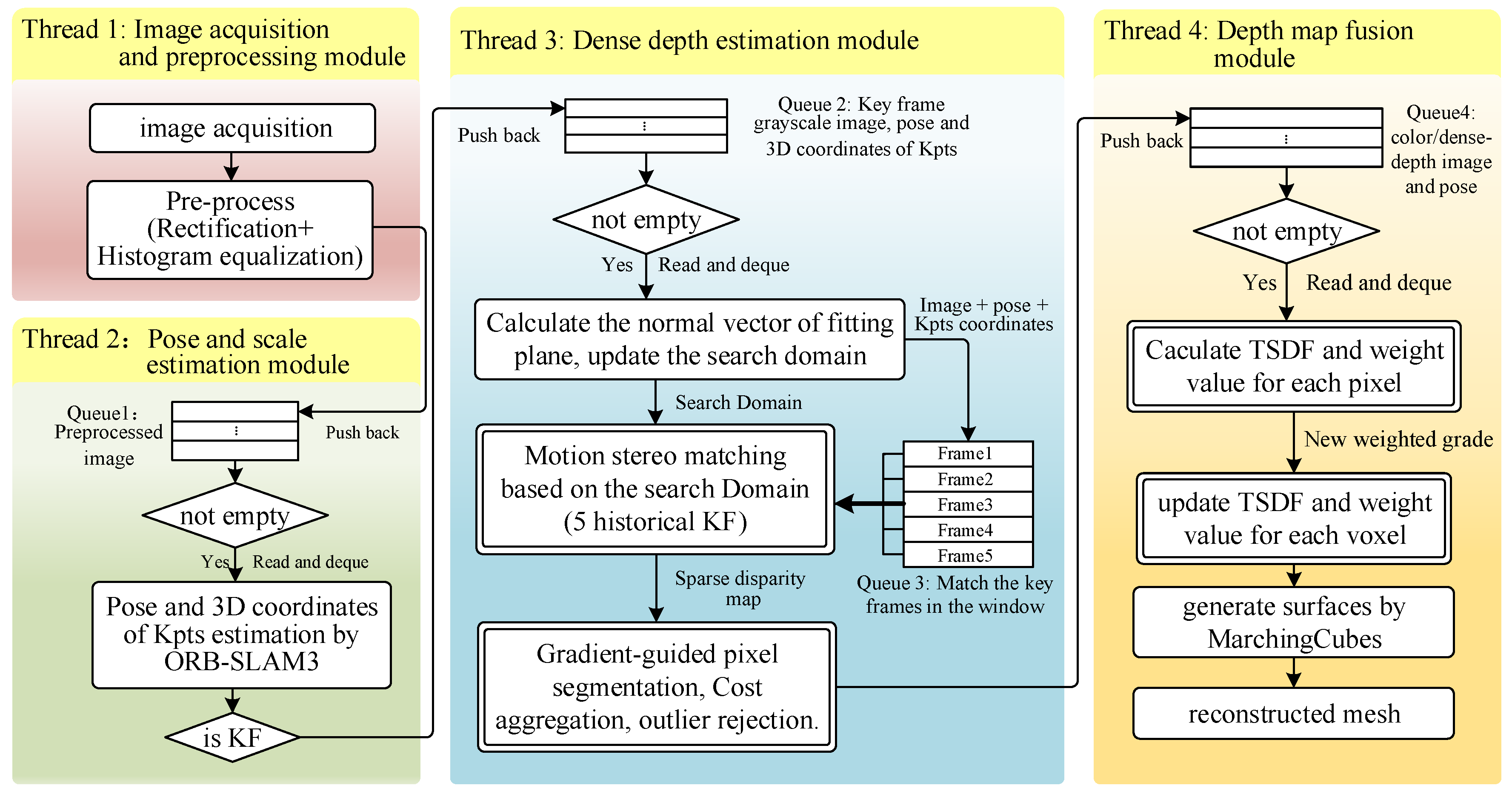
To improve the efficiency and maintainability of the proposed 3D reconstruction system, the framework is divided into several modules by using a multi-processing architecture based on a distributed robot operating system (ROS). The pipeline of our system is shown in Figure 1. It consists of four process modules: image acquisition and pre-processing module, pose and scale estimation module, dense depth estimation module, and global fusion module. Each processing module is assigned to an independent thread.

In this pipeline, modules can perform its functions in parallel and interact with each other through the data queue, which is filled with a ROS-based callback function. The image acquisition and pre-processing module acquire the image in real-time and pre-process it by un-distortion and histogram equalization for stable photometric. Pre-processed grayscale images will be pushed into the back of queue 1. Subsequently, the pose and scale estimation module gets the newest frame from the front of queue 1, and de-queue that frame to keep the size of the queue constant. Then, this module outputs the pose and 3D coordinates of the keypoints (kpts) by using ORB-SLAM3, which involves the process of ORB feature extraction and matching, triangulation, and BA optimization. Keyframe (KF) sets in queue 2 for depth estimating are selected by dynamic baseline constraint, which will be described in Section 3.2. The dense depth estimation module is mainly implemented on GPU. This module generates a dense depth map by using the proposed dynamic searching plane method and will be described in Section 3.3. At last, the final global map is obtained by fusing the incremental local depth measurements in a memory-efficient way by using a truncated signed distance function (TSDF) proposed by Zeng et al. [40]. The process marked with a double-line frame indicates that it is divided into the pixel-by-pixel calculation and implemented based on the parallel computing framework of the compute unified device architecture (CUDA). Such highly parallelized design enables the operation accelerated to achieve real-time performance, and will be described in Section 3.3.3.

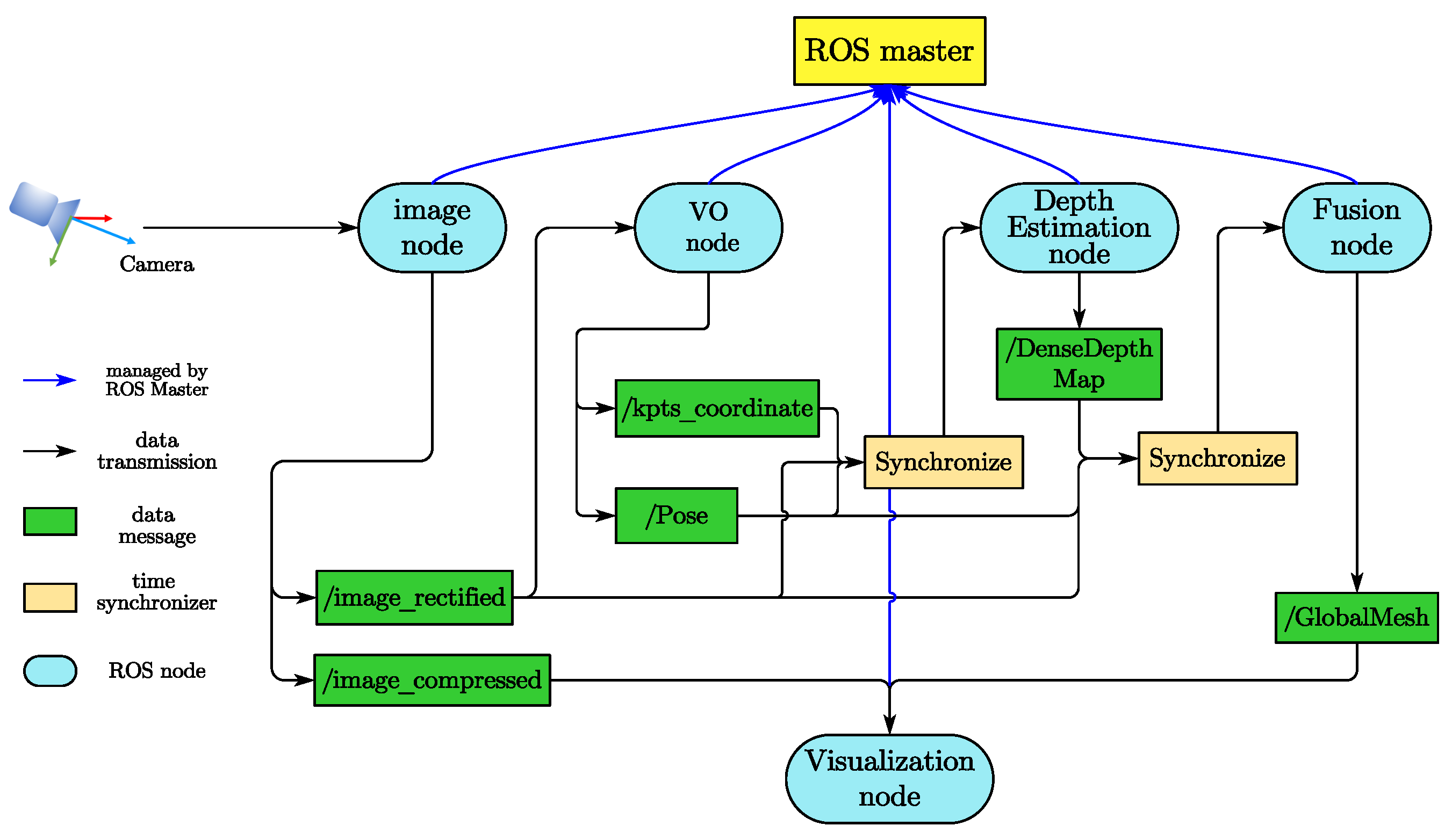
The workflow of ROS-based message passing and synchronizing is shown in Figure 2, which is a peer-to-peer network of processes that are loosely coupled using the ROS communication infrastructure. This framework can balance the computing load in performing communication and messaging passing.

3.2. Dynamic Baseline Keyframe Selection

In this section, we describe how to select the measurement frame set, which is the basis of the sliding-window-based depth estimation. The pose and scale estimation module utilized ORB-SLAM3 to calculate the relative pose of the latest frame and the 3D coordinate of the sparse feature points. The relative pose reflects the displacement and the orientation angle of the camera, and the sparse feature point clouds reflect the primary contour and the structural characteristics of the current scene. This information guided the keyframe selection method to decide whether to insert the latest frame to the measurement frame set for depth estimating. In this study, care has been taken to select the keyframe to reduce redundancy among consecutive frames and keep the parallax sufficiency among frames in the measurement set.

The relationship between the keyframe baseline length, scene depth distribution, and the accuracy of depth estimation is described below: let $e_d$ be the parallax error, $e_z$ be the depth error, b be the baseline, f (in pixels) be the focal length, and z be the depth. To facilitate the analysis, we assume that the camera movement is a lateral translation and only consider the translation vector t. Taking the first order Taylor series approximation about $e_d$ = 0, the depth error can be written in terms of the disparity error $e_d$:

$$e_z=\frac{bf}{d}-\frac{bf}{d+e_d}\approx \frac{e_d{z}^2}{bf}$$

(1)

assuming that the baseline, focal length, and parallax as constant, the depth error has a quadratic relationship with depth [41], which indicates that careful selection of baseline constraint to filtering out some frames can, therefore, effectively improve the accuracy of depth estimation. The larger the baseline, the smaller the depth error. However, a baseline threshold should be set to avoid a low percentage of overlap. Unlike most other 3D-reconstruction methods, simply set the baseline threshold as a constant or sets as dynamic but missing the geometric structure of the scene, we select the frame according to the center and the normal vector of the scene to achieve disparity stability and sufficient overlap. Thus, we proposed the following cost function:

$$cost(i)=\left|sh(1+\sin \left(\phi \right))-\frac{b^{i}f}{z_{avg}^{ref}}\right|+\left|r\tan \left(\frac{4{\alpha }^i}{\pi }\right)\right|$$

(2)

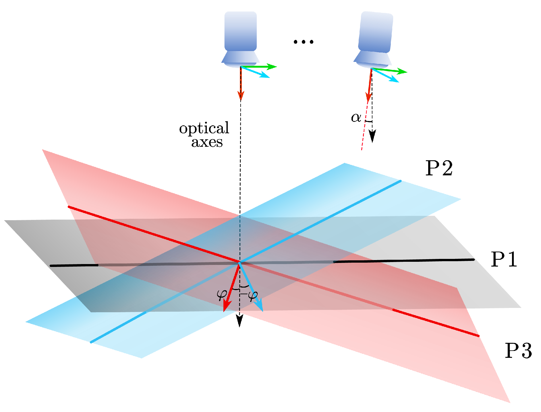
where s and r are the constant scale factor, we set to 0.25 and 0.125, respectively, as a rough indication of the intended overlap between the two images. h is image height, $\alpha$ is the optical axis angle deviation from the last KF, and $\phi$ is the angle between optical axes and normal vector $\mathit{n}$ of the fitting plane, which will be described later in Section 3.3. The first term in Equation (2) indicates that the cost function penalizes deviations from the desired disparity. Thus, the preferred next KF satisfies the disparity constrain that make the cost minimum, such that the average disparity is approximately equal to $sh(1+\sin \left(\phi \right))$. The scene can be classified into three cases according to the scale trends, as demonstrated in Figure 3. When the scene is almost parallel to the camera plane (i.e., the scene P1), φ is close to 0 such that the desired baseline is close to $sh\frac{z_{avg}^{ref}}{f}$. In other cases (i.e., the scene P2 and P3) the desired baseline of the next keyframe dynamically adjusted according to φ to achieve scale consistency and higher accuracy. In addition, since large rotation of the camera may result in insufficient overlapping, the second term of our cost function takes into account the rotation component. KF baseline becomes longer as the camera rotates or the average depth become smaller.

3.3. Multi-View Stereo Matching

In this section, we will first describe the sliding-window-based depth estimation and explain how we dynamically select a searching plane to construct a disparity matching cost vector. Then, we will describe the architecture design of embedded-GPU-based parallel-computation technology for depth-estimate acceleration.

3.3.1. Notation

Let $T_{w,c}\in \mathbb{S}\mathbb{E}\left(3\right)$ be the pose of the camera with respect to the world frame. Similarly, $T_{w,r}$ and $T_{w,k}$ be the pose transformation from reference frame and keyframe to the world frame, respectively. A landmark $P={[x, y, z]}^{\mathrm{T}}$ in 3D space is projected into the pixel coordinate through the perspective projection mapping $\mathit{u}=\pi (\overline{P})={(K{[x/z y/z 1]}^{\mathrm{T}})}_{0:1}$, where $\overline{P}$ is the normalized homogeneous coordinates corresponding to P, K is the camera intrinsic matrix. Accordingly, $\overline{P}={\pi }^{-1}\left(\mathit{u}\right)$ represents the inverse process of projection. To simplify the expression, use ${(·)}_{0:1}$ denotes the vector formed by the first two element of the vector $(·)$. ${\mathsf{\Gamma }}_{\mathit{n},P}$ denotes a plane with interior point P and normalized vector n.

3.3.2. Matching Cost

The first step of depth estimation processing workflow involves maintaining a fixed size queue of recent KFs $I_r\in \mathcal{R}$, which are candidates for multi-view stereo matching. Such a fixed-size queue is a sliding window. The new keyframe $I_k$ satisfying the baseline constraint will be added to the back of this queue. Then, the window shifts forward to delete the oldest frame so that we can maintain sufficient parallax and constant computational complexity.

The relative pose from $I_r$ to $I_k$ estimated by the pose estimation module will be used for triangle constraint to recover depth of pixels in $I_k$. The most important step in this process (i.e., depth estimate) is to correctly match corresponding pixel in multi-view frames. Like other direct or semi-direct method based SLAM, we assume that the imaging intensity value corresponding to a certain 3D landmark in space remains constant in all observations. Such an assumption is called pixel grayscale invariance [42]. To eliminate the impact of illumination change or intensity noise on pixel matching, we consider the patch-pixel grayscale invariance, i.e., matching the similarities of a $n\times n$ patch window instead of one single pixel. Given a certain depth hypothesis of a pixel in $I_k$, by projecting the corresponding 3D coordinate to all candidate matching frames $I_r\in \mathcal{R}$, we can obtain the matching cost by measuring the intensity difference. The process of depth search equivalent to minimizing the matching cost.

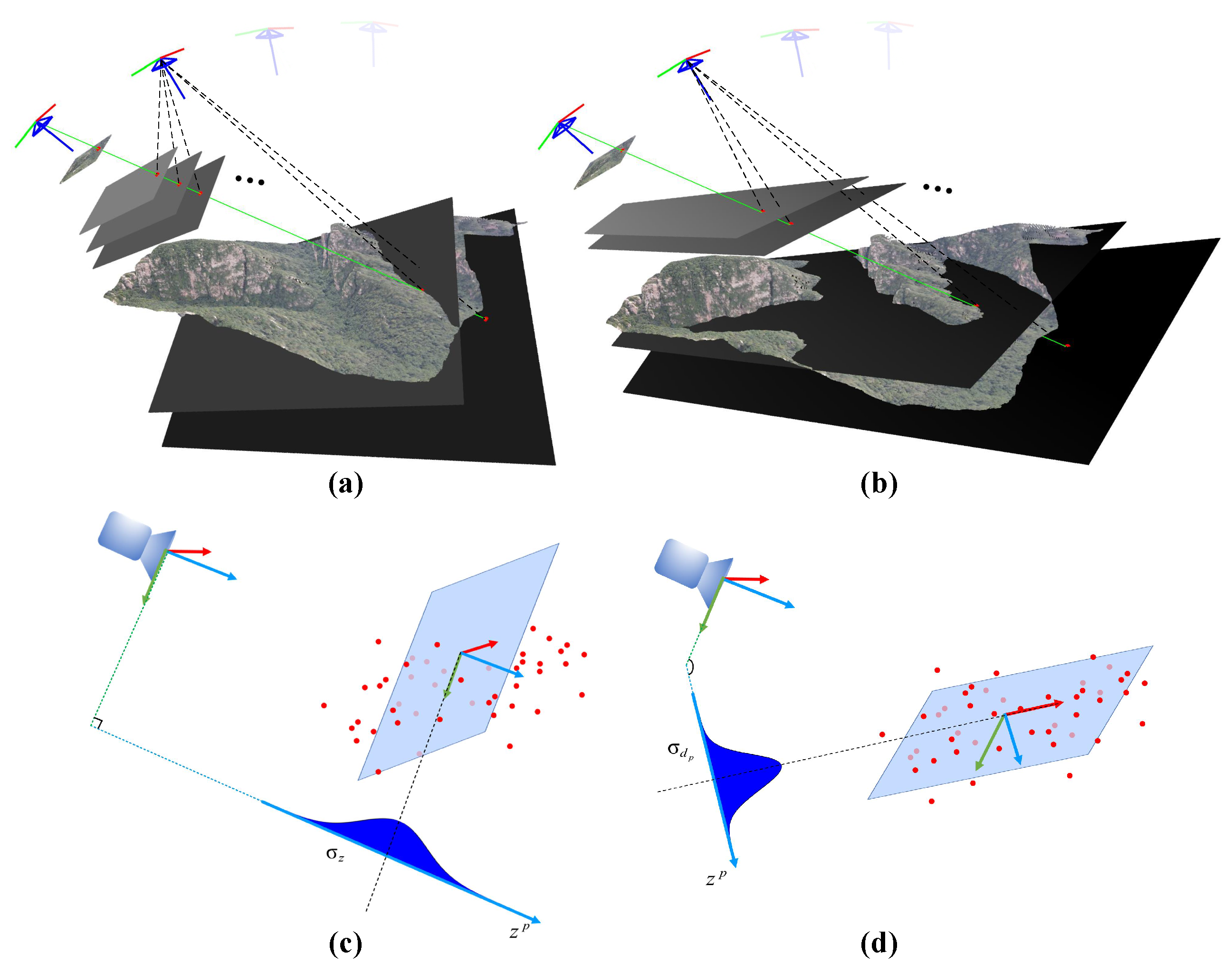
In stereo matching, each selected point in $I_k$ is sampled by N_d depth values, which are uniformly distributed in certain depth space. The sampling depths of all pixels constitute N_d depth searching planes. Those depth values are used as the hypothesis for calculating the matching cost in candidate reference frames one by one. The final value of depth measurement $z^{*}$ is determined by the minimum matching cost. Since the resolution of depth estimation is decided by the distance between neighboring searching planes, elaborately selecting depth planes is therefore crucial to depth estimation accuracy. A comparison of the selected depth searching plane is demonstrated in Figure 4. Unlike the other methods, which selecting planes parallel to the imaging plane (i.e., (a,c) in Figure 4), our method allows the plane to be selected with significant flexibility by dynamically fitting the spatial distribution of depth.

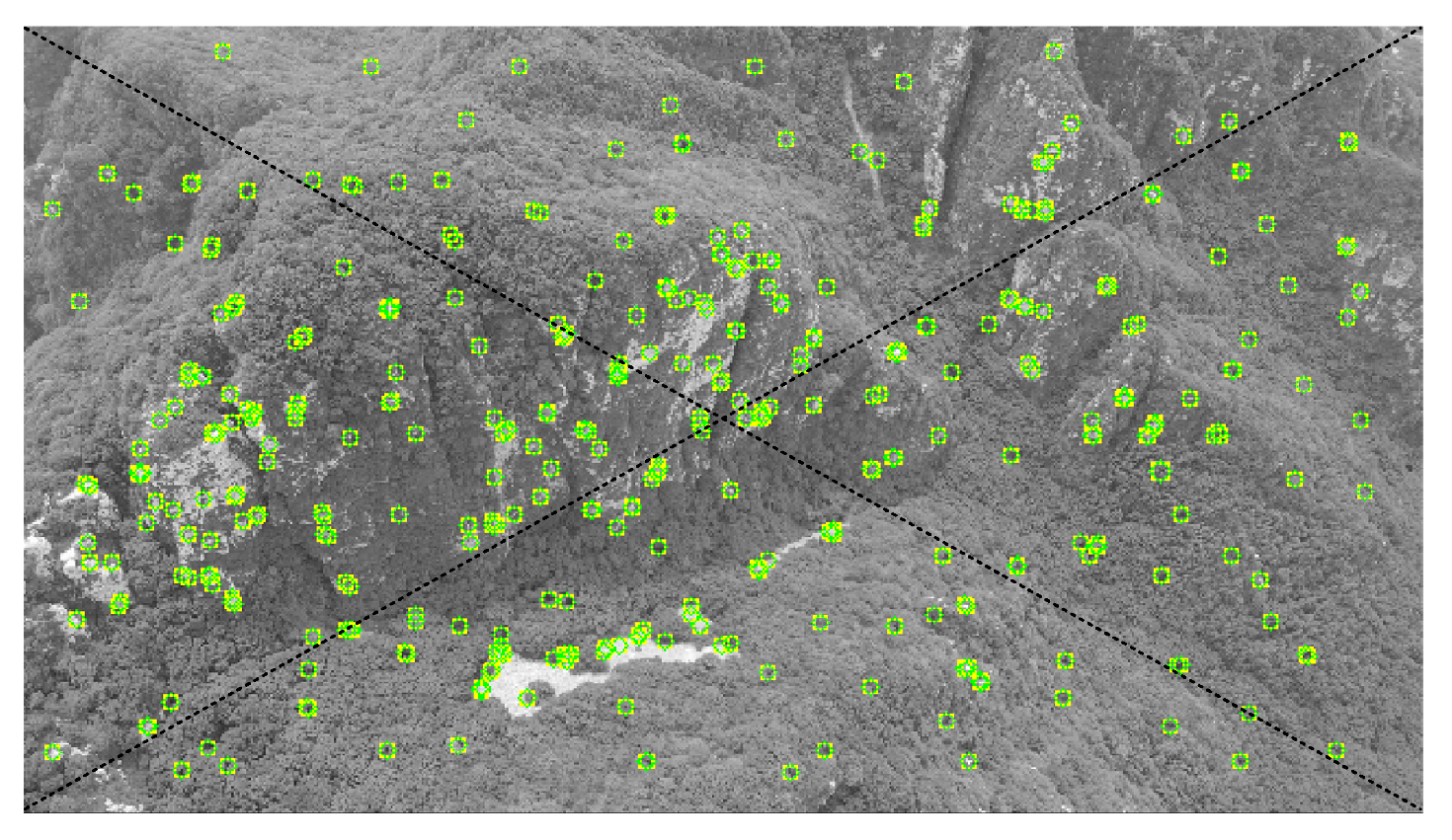
Three-dimensional coordinates of keypoints calculated by BA are used as a prior to predict the spatial distribution of depth in the scene. Figure 5 shows that the distribution of the keypoints extracted by ORB-SLAM3 is divided into four areas. Let $P_m={\left[x_m y_m z_m\right]}^{\mathrm{T}}$ be the focus of the whole scene, and the focus of each area is $P_i={[x_i y_i z_i]}^{\mathrm{T}},i=0,1,2,3$, which can be obtained by calculating the mean 3D coordinates of keypoints in each area. The depth distribution of the scene can be approximated by a fitting plane ${\mathsf{\Gamma }}_{\mathit{n},P_m}$, which passes through the focus $P_m$, and its normal vector $\mathit{n}={[a b c]}^{\mathrm{T}}$ satisfies:

$$\left(\begin{array}{c}{x}_1-x_m y_1-y_m z_1-z_m\\ x_2-x_m y_2-y_m z_2-z_m\\ x_3-x_m y_3-y_m z_3-z_m\\ x_4-x_m y_4-y_m z_4-z_m\end{array}\right) \left(\begin{array}{c}a\\ b\\ c\end{array}\right)=A\mathit{n}=0$$

(3)

where $\mathit{n}$ can be obtained by using SVD decomposition of A, such that the equation of the fitting plane is defined as:

$${\mathsf{\Gamma }}_{\mathit{n},P_m}(x,y,z):a(x-x_m)+b(y-y_m)+c(z-z_m)=0$$

(4)

For a given pixel, p with normalized homogeneous coordinates $\overline{P}$, let $\gamma$ be the optic ray (i.e., the green line in Figure 4) that passes through both the optical center and $\overline{P}$, finding the 3D coordinates $P={(x y z)}^{\mathrm{T}}$ of the selected point is equivalent to solving the intersection point of $\gamma$ & ${\mathsf{\Gamma }}_{\mathit{n},P_m}$, which yields:

$$\frac{x}{{\overline{P}}_x}=\frac{y}{{\overline{P}}_y}=z$$

(5)

Combining Equations (4) and (5), we can solve the candidate depth value on the searching plane corresponding to $\overline{P}$ by:

$$z_{\mathit{n},P_m}(\overline{P})=\frac{a{x}_m+b{y}_m+c{z}_m}{a{\overline{P}}_x+b{\overline{P}}_y+c}=\frac{\mathit{n}{P}_m^{\mathrm{T}}}{\mathit{n}{\overline{P}}^{\mathrm{T}}}$$

(6)

Distance between the fitted 3D feature point ${\mathrm{P}}_f$ and the fitting plane $\mathsf{\Gamma }(\mathit{n},{\mathrm{P}}_m)$ are calculated by:

$$d({\mathrm{P}}_f,\mathsf{\Gamma })=\frac{{\mathsf{\Gamma }}_{\mathit{n},{\mathrm{P}}_m}\left({\mathrm{P}}_f\right)}{\sqrt{\Vert \mathit{n}\Vert }}$$

(7)

We assumed that $d\left({\mathrm{P}}_f,\mathsf{\Gamma }\right)$ obeyed the normal distribution with covariance ${\sigma }_{d_p}$. Hence, take $({\mathsf{\Gamma }}_{\mathit{n},P_m-3{\sigma }_{d_p}·\mathit{n}},{\mathsf{\Gamma }}_{\mathit{n},P_m+3{\sigma }_{d_p}·\mathit{n}})$ as the search range, as demonstrated in Figure 4b, the N_d candidate depth values of all pixels uniformly covered the whole scene. For any given pixel ${\mathit{u}}_k$ in frame $I_k$, the corresponding candidate depth $d\left({\mathit{u}}_k,i\right)$ is calculated by:

$$d({\mathit{u}}_k,i)=z_{\mathit{n},P_i}\left({\pi }^{-1}{({\mathit{u}}_k)}_{0:1}\right)$$

(8)

$$z_{\mathit{n},P_i}(\overline{P})=\frac{\mathit{n}{(P_m+\frac{2i-N_d}{N_d}3{\sigma }_d·\mathit{n})}^{\mathrm{T}}}{\mathit{n}{\overline{P}}^{\mathrm{T}}},i=0,1,\dots ,N_d-1$$

(9)

where the sequence of $d({\mathit{u}}_k,i)$ for $i=0,1,\dots ,N_d-1$ denotes the set of candidate depth in the searching planes. Then, we can get a set of matching 2D points, denoted as ${\mathit{u}}_r^{prj}$, located in sliding window frames (i.e., history keyframe in $\mathcal{R}$) by coordinate transform and projection process:

$${\mathit{u}}_r^{prj}=\pi \left(T_{w,r}^{-1}{T}_{w,k}d({\mathit{u}}_k,i){\pi }^{-1}({\mathit{u}}_k)\right)$$

(10)

As mentioned above, by measuring the intensity difference, we can obtain the matching cost vector:

$$C({\mathit{u}}_k,i)=\frac{1}{\left|\mathcal{R}\right|}\mathrm{\sum }_{I_r\in \mathcal{R}}SAD\left(I_r,I_k,{\mathit{u}}_k,d({\mathit{u}}_k,i)\right)$$

(11)

where $SAD$ simply calculates the sum of absolute difference of two 3 × 3 pixel patches located at ${\mathit{u}}_k$ and ${\mathit{u}}_r^{prj}$:

$$SAD\left(I_r,I_k,{\mathit{u}}_k,d({\mathit{u}}_k,i)\right)=\left|I_r\left({\mathit{u}}_r^{prj}\right)-I_k({\mathit{u}}_k)\right|$$

(12)

3.3.3. Parallel Computing

In this section, we described the detailed implementation in the process of depth searching. Since the calculation of matching cost between pixels is independent of each other, for the benefit of online computation, we implement every cost calculation in GPU as an independent thread to accelerate the process.

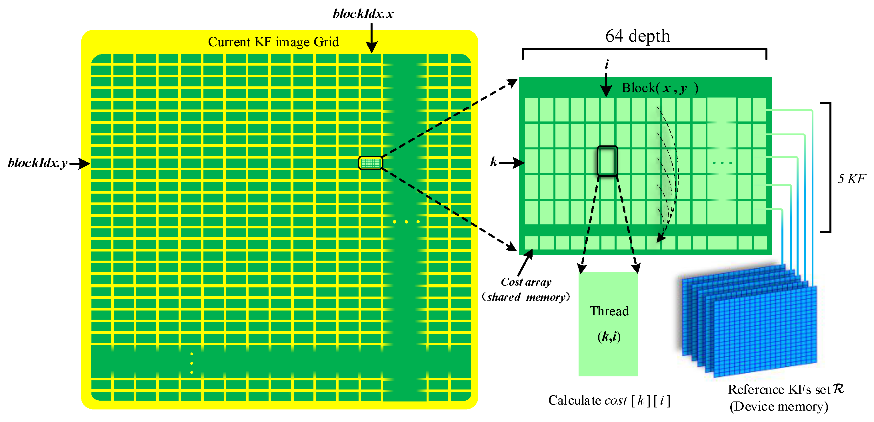
As shown in Figure 6, the current matching image grid is composed of multiple CUDA blocks, and each CUDA block is composed of multiple threads, enumerating $N_d$ depth hypothesis. In each block thread, the matching cost of a $4\times 4$ pixel patch in all measurement frame $\mathcal{R}$ is carried out independently for $N_d$ depth hypothesis, which means that a block contains $\Vert \mathcal{R}\Vert \times N_d$ threads. We sum the cost result of different threads for each depth hypothesis and write the results to an $N_d$ array in shared memory, which multiple threads can access. The final optimal depth $d^{*}$ is determined by the minimum matching cost:

$$\arg \underset{d^{*}}{\min }\mathrm{\sum }_{k=1}^{\Vert \mathcal{R}\Vert }cost(k,d)$$

(13)

In CUDA architecture, the smallest computing unit of a warp contains 32 threads [43]. Considering both the memory and computation time, we set the number of historical keyframes in the sliding window as 5, and set the number of depth hypothesis as $N_d$ = 64. Each block has 320 threads, which is the integer multiple of 32. The final cost is a 64 dimension array, which is stored in the shared memory of the block and can be accessed by all block threads. The calculation of each block thread is as shown in Algorithm 1.

Algorithm 1 Pseudocode of optimal depth extraction algorithm.

Input:

1: blockIdx;

2: threadIdx;

3: image intensity of current target keyframe $I_k$ and measurement frame set $I_r\in \mathcal{R}$

Output: optimal $d^{*}$

4: Pixel col: $x\leftarrow 4\times blockIdx.x$

5: Pixel row: $y\leftarrow 4\times blockIdx.y$

6: Currently matched referent keyframe index: $r\leftarrow threadIdx.x,r\in [0,\Vert \mathcal{R}\Vert ]$

7: Currently matched depth hypothesis index: $i\leftarrow threadIdx.y,i\in [0,N_d-1]$

8: define shared memory array: $cost\left[N_d\right]\leftarrow \mathbf{0}$     ⊳ Accessed by all block threads

9: define shared memory array: $depth\_index\left[N_d\right],depth\_index\left[i\right]\leftarrow i$

10: define local variable: $\Delta I\leftarrow 0$

11: ${\mathit{u}}_k\leftarrow (x,y)$

12: $d({\mathit{u}}_k,i)\leftarrow$ Equation (8)

13: ${\mathit{u}}_r^{prj}\leftarrow$ Equation (10)

14: for $patch\_i=-1$; $patch\_i<2$; $patch\_i++$ do

15:  for $patch\_j=-1$; $patch\_j<2$; $patch\_j++$ do

16:   $\mathit{p}\leftarrow (patch\_i,patch\_j)$

17:   $\Delta I\leftarrow \Delta I+\left|I_r({\mathit{u}}_r^{prj}+\mathit{p})-I_k({\mathit{u}}_k+\mathit{p})\right|$

18:  end for

19: end for

20: $cost\left[i\right]\leftarrow cost\left[i\right]+\Delta I$        ⊳ Avoid thread blocking by using atomicAdd()

21: synchronize threads

22: $step\leftarrow N_d/2$

23: for $step>0$ do

24:  if $i<N_d/2$ and $cost\left[i\right]>cost[i+step]$ then

25:   $cost\left[i\right]\leftarrow cost[i+step]$                ⊳ Parallel rolling scan

26:   $depth\_index\left[i\right]\leftarrow i+step$

27:  end if

28:  $step\leftarrow step/2$

29:  synchronize threads

30: end for

31: $i^{*}\leftarrow depth\_index\left[0\right]$

32: $d^{*}\leftarrow d({\mathit{u}}_k,i^{*})$

By using parallel acceleration and rolling scan strategy, we reduced the time complexity of Equation (13) from $O\left(N_d^2\right)$ to $O\left(log\left(N_d^2\right)\right)$ in our algorithm, and extract the optimal depth for each pixel patch in each keyframe with the highest efficiency.

4. Experiment and Results

In this section, we present the evaluation comparison between the proposed method and other state-of-art methods: REMODE [44], probabilistic-mapping [45], and quadtree-mapping [39]. Those methods are targeted on dense depth estimation on portable devices. The system is evaluated in the following three aspects:

• Accuracy: The relative error rate (% w.r.t m), RMSE(m), and mean error(m) were calculated for the cross-method evaluations;
• Computation time (ms): The average computation time of each selected keyframe and the total computation cost;
• Density rate (%): The average percentage of the valid measurement in each depth map.

Two types of experiments were carried out. The first experiment was a depth accuracy evaluating experiment in which synthetic aerial images and ground truth depth are used. The second experiment used real large scene aerial video for time consumption and stable performance evaluation of the system. In addition, we have quantified the difference between the models generated by our system and commercial reconstruction software under real scene data.

The system was implemented using C++/CUDA on the embedded platform NVidia TX2 [46], which is equipped with a quad-core ARM CPU and a 256-core GPU, 8 GB of memory, and its excellent SWaP (Size Weight and Power) capability makes real-time dense reconstruction of portable platforms possible. All the experimental for this study are carried out based on this platform.

4.1. Accuracy Evaluation

4.1.1. Evaluation Data Acquisition

The popular RGB-D datasets, such as the TUM RGB-D SLAM dataset [47], ICL-NUIM dataset [48], and KITTI dataset [49], were originally designed for odometry, thus they are not suitable for the evaluation of 3D reconstruction algorithm, especially for algorithms designed for large-scenes. Moreover, error of depth obtained by the binocular camera is non-negligible in the large scene. Therefore, it is difficult to obtain the depth ground-truth of the real large scene. We proposed an experimental approach for evaluating the depth accuracy based on synthesized data, which is generated by the Gazebo 3D robotics simulator [50]. To make the synthesized data more realistic, the virtual scene is build up by sunlight conditions and certain textures that are typically observed in the real world, such as grass, sands, and rocks, as shown in Figure 7. Besides, simulated RGB-D sensor in this environment can provide perfect depth ground-truth corresponding to each RGB image.

As is shown in Figure 8a,b, an 16-bit grayscale depth map with a spatial resolution of 1 m were obtained by height map generator: terrain.party [51] (data sourced by OpenStreetMap [52]) from the real-world. This height map enables us to build a real-scale uneven terrain 3D model with the size of 8000 m × 8000 m in the Gazebo simulator. We use a simulated s UAV equipped with an RGB-D camera to fly over the scene and acquire the aerial data. The RGB images are used for system input and the depth maps for accuracy evaluation. Furthermore, the ground truth pose is given. By modeling sensor noise in the RGB camera, real-world artifacts in the synthesized data are simulated. Besides, the simulation environment can provide the physical characteristics of the wind so that the UAV can swing weakly within the controllable range.

In the photogrammetric terrain mapping tasks, aerial images are usually taken at different ground heights for the various types of terrain. Considering this, we take the UAV flight height and the average height difference of terrain as variables to design two kinds of datasets for accuracy evaluation. The flight height is the average distance between the UAV and the ground, and the height difference of terrain is the distance between the highest and lowest points of the terrain in a top view.

The first dataset contains aerial images captured at different ground heights (800 m, 1000 m, and 1200 m) for the same scene. We built a terrain based on the height map shown in Figure 8 for this dataset. For the second dataset, we built three new height maps with different height differences (100 m, 200 m, and 300 m). The front view and the side view of the three scenes are shown in Figure 9. We fixed the relative flight height of the UAV as 300 m to collect the data. To make the experiment unaffected by other factors, the scene texture mapping used in each case is the same. Figure 10 shows some example images of the two datasets taken at different spatial positions.

4.1.2. Depth Accuracy Evaluation

The synthesized datasets described in Section 4.1.1 are used for cross-method accuracy evaluation. All algorithms compared in this experiment use the pose generated by ORB-SLAM3 as the mapping pose. After obtaining the depth maps, the accuracy assessment procedures were performed. All six image sequences were compared by using the relative error rate and root mean square errors (RMSE) of estimated depth.

Since the monocular based visual odometry cannot recover the absolute scale of the pose, depth value estimated by multi-view geometry is proportional to the true value under a scale factor. To evaluate the depth accuracy in the true scale, we use the scale w.r.t. the ground-truth translation vector t to scale the depth. Considering that the depth map is generated between the current KF and the measurement frames in $\mathcal{R}$, set the scale average of the corresponding pose t as the zoom factor $s_k$ of the depth in frame k:

$$s_k=\frac{1}{\Vert \mathcal{R}\Vert }\sum _{i\in \mathcal{R}}\frac{\Vert t_{ik}^{gt}\Vert }{\Vert t_{ik}^{est}\Vert }$$

(14)

such that the relative error rate of pixel depth in depth map $D_k$ is defined as:

$$e_r=\frac{|s_k·d_p^{est}-d_p^{gt}|}{d_p^{gt}},p\in D_k$$

(15)

and the depth RMSE is calculated by:

$${\mathrm{RMSE}}_{(d)}=\sqrt{\frac{1}{n}\sum _{D_k\in \mathcal{R}}\sum _{p\in D_k}{(s_k·d_p^{est}-d_p^{gt})}^2}$$

(16)

The result is shown in Figure 11, a comparison of pixel percentage of converged measurements (vertical axis) within a certain relative error rate threshold (horizontal axis).

The curves shown in Figure 11 described the distribution of the estimated values of the algorithm in different accuracy ranges. The corresponding detailed numerical values statistics is shown in

Table 1. Detailed numerical values statistics of results of different methods on the synthesized datasets. The best metric value is highlighted in bold.

Method	Metrics	Flying Ground Height			Terrain Height Difference
		800 m	1000 m	1200 m	100 m	200 m	300 m
Ours	Error Rate within 1% (%)	83.741	81.542	85.974	77.273	83.791	78.389
	Outlier Rate (%)	0.706	1.227	1.261	0.612	1.347	1.682
	RMSE (m)	5.767	7.608	8.288	2.441	2.020	2.448
	Mean Error (m)	4.537	5.957	6.516	1.970	1.544	1.910
Quadtree Mapping	Error Rate within 1% (%)	82.101	77.053	80.62	69.998	74.016	76.113
	Outlier Rate (%)	0.632	1.182	0.934	0.899	1.591	0.719
	RMSE (m)	5.940	8.322	9.352	2.996	2.559	2.541
	Mean (m)	4.701	6.574	7.445	2.296	2.066	2.018
Probabilistic Mapping	Error Rate within 1% (%)	64.821	60.124	57.403	70.511	76.068	69.464
	Outlier rate (%)	3.410	6.183	9.433	2.493	2.533	3.558
	RMSE (m)	8.081	12.258	12.953	2.882	2.465	2.879
	Mean (m)	6.534	10.024	10.486	2.274	1.941	2.271
REMODE	Error Rate within 1% (%)	67.632	73.210	62.288	69.086	76.842	69.419
	Outlier rate (%)	5.113	2.760	13.641	3.3186	1.874	2.610
	RMSE (m)	7.839	9.136	11.223	2.985	2.428	2.836
	Mean (m)	6.168	7.106	9.016	2.348	1.949	2.280

. The results indicate that for low altitude and highly uneven terrain, the performance of different algorithms tends to be relatively close. While for the flatter and further terrain, adjusting the matching baseline and using planar features of the scene enable our algorithm to outperform the others in insufficient parallax cases. We achieved over 81% of estimated depth with error rate less then 1% in this case. For the lower altitude (300 m) data with different flatness, we achieved typical RMSE of depth error around 2.3 m.

4.2. Global Mapping Evaluation

In the last evaluation experiment, we measured the accuracy of each depth estimation, i.e., the accuracy of Z. For the 3D point, which can reflect the accuracy in terms of X, Y, and Z three dimensions, we evaluated by the global mapping in this section.

The 3D point cloud generated in this study is originally from the 2D depth map. By applying mapping transformation through the camera pose, and marginalizing the redundant estimation by using TSDF, we can build a global map of the entire scene. Depth maps stability (i.e., consistency of the estimate for the same spatial object point in different keyframes) plays an important role in this step. We project all the depth maps to the spatial, as is shown in Figure 12, to evaluate the point cloud stability.

Purple boxes in Figure 12a,b shows the comparison of the reconstructed point cloud details in the case of an inclined scene. Due to the change of scale and the lack of parallax of distant points, REMODE has more noise than ours because it cannot maintain the depth stability of the same 3D landmark in different observations. Moreover, the point cloud density at the edge of the scene is significantly reduced. Our method adjusts the search range of different areas to be as close to the scene depth as possible, enables us to achieve a smoother estimation without a filter. As for the areas of green boxes, the preset search range is too large for the estimation module of quadtree-mapping, which causes the point cloud drift in a larger range, resulting in the thick surface point cloud. As is shown of the detail in the black boxes, the probabilistic-mapping causes streak artifacts due to 4-path optimization. We use the global 2D update SGM as quadtree-mapping do so that this problem can be avoided.

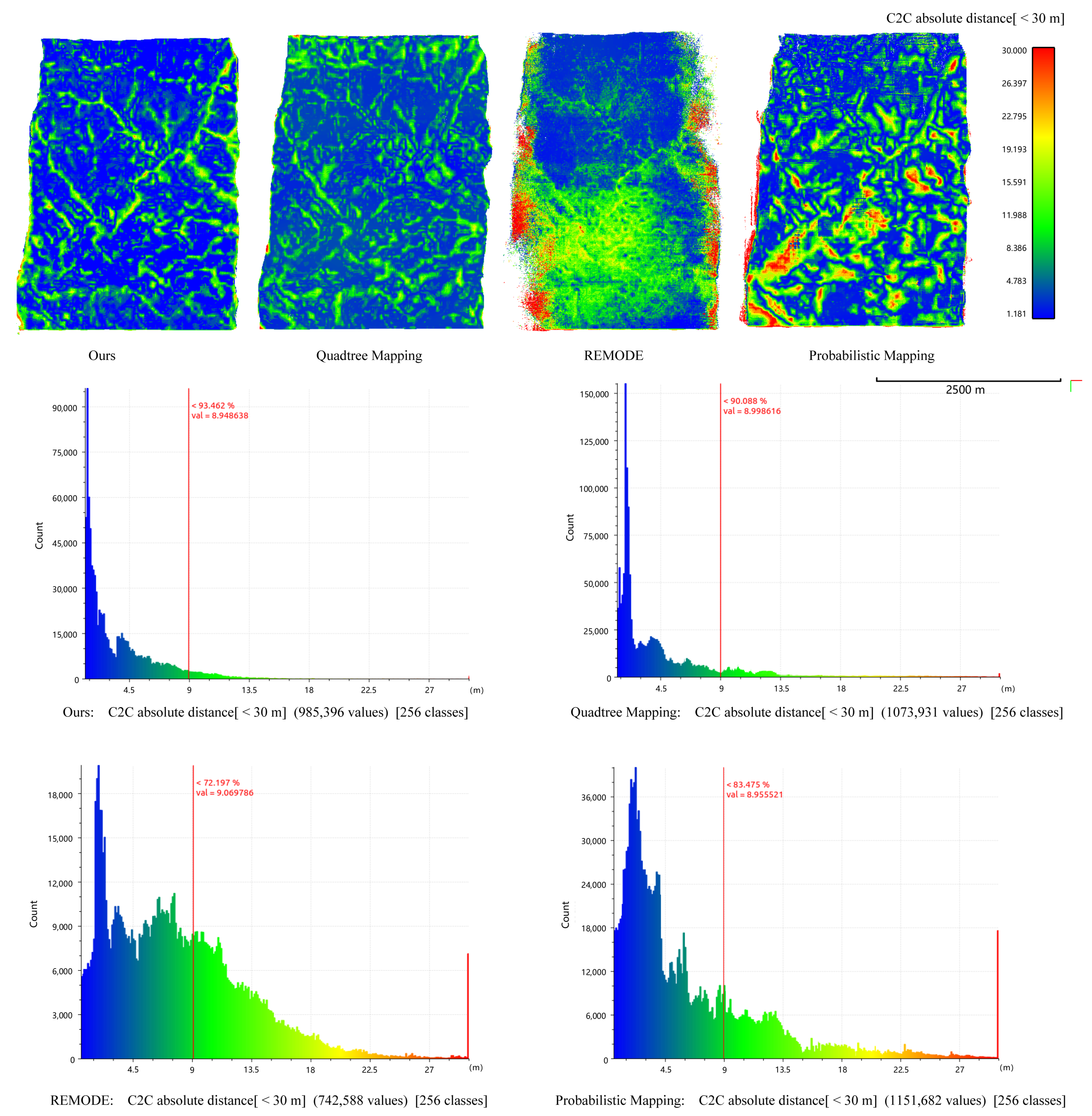
The data used in this experiment is the 1000 m height sequence of dataset 1, and the rest of the datasets produced similar results. The C2C (Cloud to Cloud) absolute distance error of the final terrain model was carried out using CloudCompare [53] open source software. The CloudCompare is a 3D processing tool, also known as a evaluation tool, which calculates the closest distance between each estimated point and the ground truth point cloud. We set the distance threshold as 30 m, and the error map and respective absolute error distribution histogram is given.

As the error pseudo-color map illustrated in Figure 13, the proposed method can maintain stable estimation accuracy in different areas of scene scale change. On the other hand, we can see that the estimation accuracy is more improved than single depth map after depth fusion. Our method achieves percentage of absolute distance error lower then 9 m (0.9% of the absolute distance) is 93.462%, quadtree-mapping 90.088%, REMODE 72.197%, and probabilistic-mapping 83.475%.

4.3. Speed Evaluation

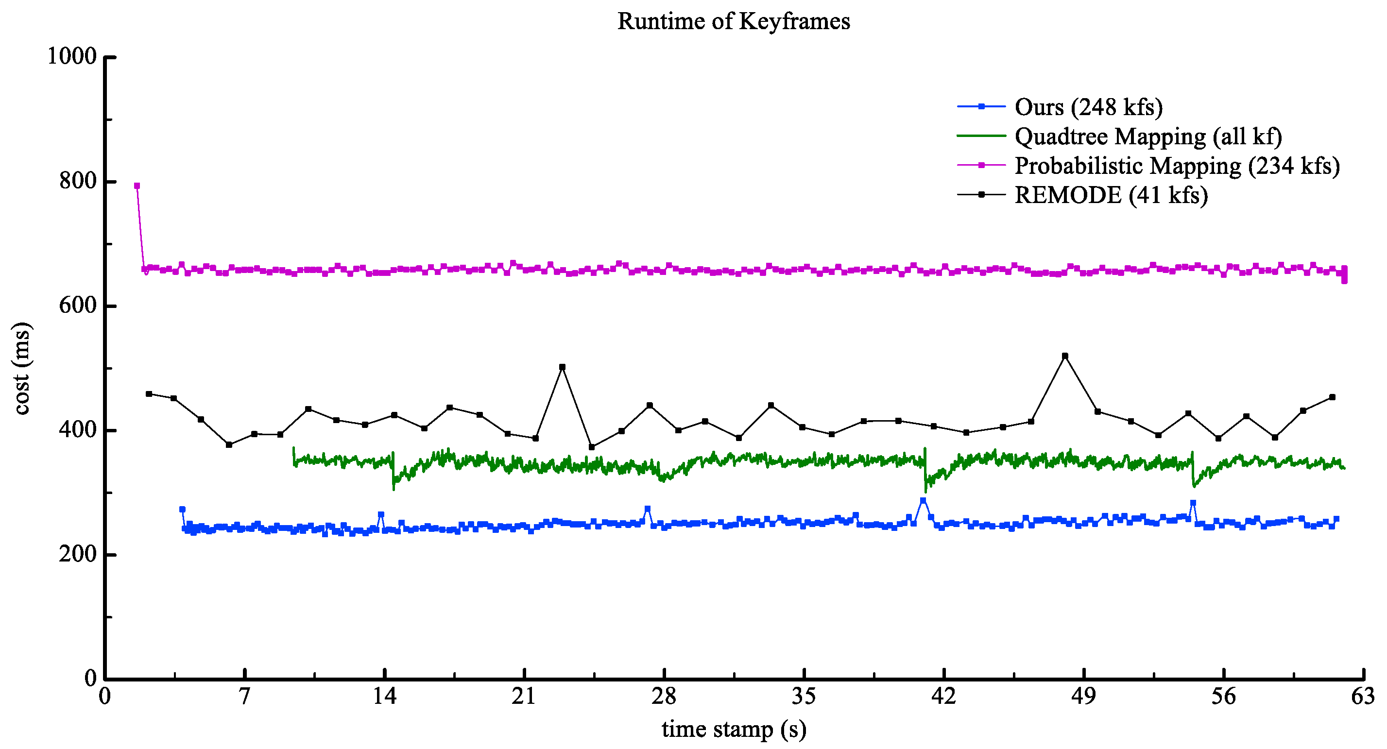
We compared our method with the other three methods: REMODE, probabilistic-mapping, and quadtree-mapping in terms of run-time per keyframe to evaluate the efficiency of the proposed algorithm. This experiment is based on the aerial video captured by the DJI Air2 UAV platform at 30 fps and resized to 960 × 540 pixels. Results of keyframe computational cost as shown in Figure 14.

Probabilistic-mapping does not a have keyframe selection module, and it achieves real-time performance by abandoning presets number of the frame. Quadtree-mapping transfers the depth of each frame and iteratively updates it, enabling the system to generate dense depth for every input image in the tracking model. Hence, the run time is relatively long. The average cost and the average density rate of the depth map are shown in

Table 2. Results comparison with state-of-art method on aerial video data.

Method	Number of Keyframe	Mean Cost Per Keyframe (s)	Total Run-Time (s)	Density Rate (%)
Ours	248	0.229	62.762	93.391
Quadtree-Mapping	1577	0.346	646.999	97.189
REMODE	41	0.417	64.981	50.695
Probabilistic-Mapping	234	0.657	153.866	96.693

, and our method generates depth maps in a shorter time without losing much of the density rate.

4.4. Evaluation in Real-World Terrain Scenes

In this section, we presented the results obtained from real-world large scene to prove the usability and efficiency of our system. Since it is difficult to obtain the depth ground-truth of the real large scene, and there is no aerial datasets contain both RGB and depth images of the terrain, we chose to compare with the commercial software, PhotoScan (Agisoft LLC, Russia) [54], which is mainly targeted at the accuracy of reconstruction. It usually takes a long time to process and requires high level calculation power hardware. The surface absolute difference among the proposed methods and PhotoScan are obtained for quantitative comparison.

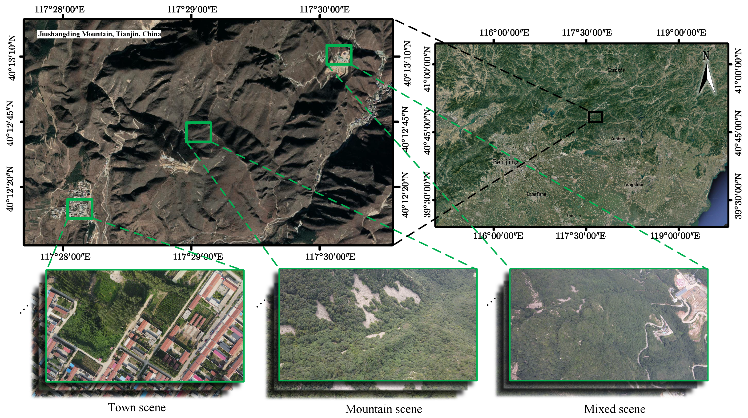
The UAV platform we used in this experiment was equipped with a UHD camera to acquire aerial images at 3840 × 2160 resolution and 30 frames per second. Besides, GPS and IMU values are also recorded, enabling us to classify the data by the approximate ground high and pitch angle (the angle between the optical axis of the camera and the horizontal plane). The UAV has flight several times to acquire aerial images on the region of interest, including town, mountain, and the mixed zone scene. These scenes located in the Jiushangding mountain, Tianjin, covering the area at approximately nine square kilometers. Figure 15 shows examples of satellite images acquired by google earth and aerial images acquired by UAV. These datasets were taken at ground heights ranging from 400 m to 1000 m in different pitch angle. Before feeding the sequences to our system, we resized all images to 960 × 540 resolution for the balance between run-time and accuracy. Detailed statistics are as shown in

Table 3. Detailed statistics of aerial datasets and results point cloud number of our method.

Image Sequences	No.	Image Amount	Approximate Ground Height (m)	Pitch Angle (°)	Point Amount
Towns	1	1811	400	75	632,758
	2	1805	500	75	596,257
	3	1823	500	90	613,125
Mountains	1	1806	600	75	563,649
	2	1851	800	75	513,699
	3	1864	800	90	533,461
Mixed Zone	1	1835	800	75	476,533
	2	1840	800	75	451,128
	3	1862	1000	90	419,561

.

In this experiment, the results of Photoscan are used as the benchmark. After obtaining the models, the ICP algorithm, implemented in CloudCompare, was used to align the model generated by our method and the model obtained by Photoscan. The absolute distance difference between the models is then calculated. Note that we only calculate the distance difference of common parts, no consideration will be given to the differences in the edges.

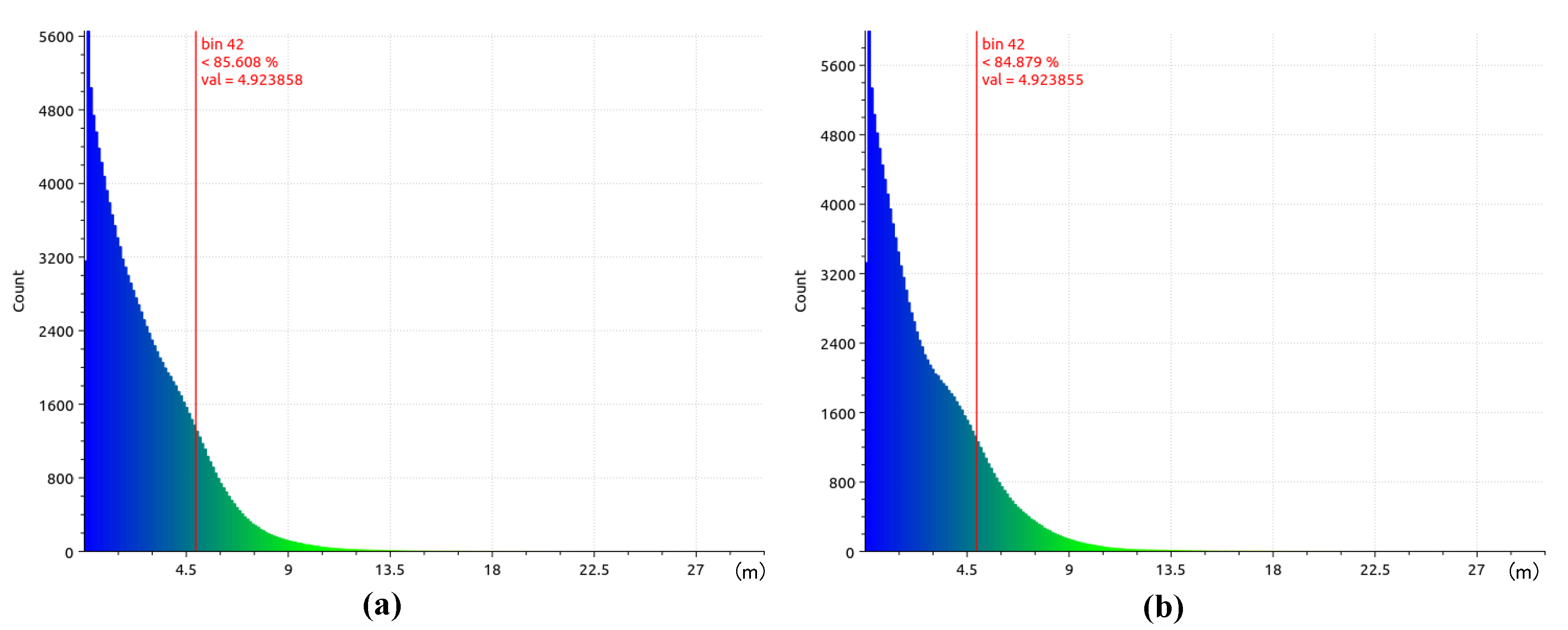
Figure 16 and Figure 17 shown two examples of reconstructed results comparison of our and Photoscan method in real-world aerial data. The surface absolute difference distribution between Photoscan and proposed method shown in Figure 18 indicate that more than 84% of sample points’ difference are less than 5 m on the 800 m flight height data Mixed Zone-2. We downsampled all the data to 960 × 540 and input the two methods for efficiency and difference evaluation. In order to make Photoscan obtain higher accuracy, the images were aligned with GPS data. Finally, the hardware environment, time consumption, and percentage of difference within 5 m of the two methods are shown in

Table 4. Time cost compare on datasets in Table 3, T is the Town, M is the Mountains, and MZ is the Mixed Zone.

Methods	CPU	GPU	Time Costs on Aerial Datasets (m′s″)
			T1	T2	T3	M1	M2	M3	MZ1	MZ2	MZ3
Ours	Arm Cortex A57	TX2 Embedded GPU	$1^{\prime }{01}^{″}$	$1^{\prime }{01}^{″}$	$1^{\prime }{02}^{″}$	$1^{\prime }{01}^{″}$	$1^{\prime }{03}^{″}$	$1^{\prime }{03}^{″}$	$1^{\prime }{02}^{″}$	$1^{\prime }{02}^{″}$	$1^{\prime }{03}^{″}$
Photoscan	Intel Core i9 10850	NVidia RTX2080ti	${37}^{\prime }{50}^{″}$	${30}^{\prime }{17}^{″}$	${34}^{\prime }{45}^{″}$	${29}^{\prime }{14}^{″}$	${26}^{\prime }{32}^{″}$	${30}^{\prime }{37}^{″}$	${25}^{\prime }{43}^{″}$	${25}^{\prime }{58}^{″}$	${27}^{\prime }{51}^{″}$
Percentage of Difference < 5 m(%)			75.31	78.23	81.27	81.68	83.14	88.25	83.85	84.87	89.25

.

In summary, for real-world aerial images with a flight height of about 500 m, more than 75.3% of our estimated point cloud are less then 5 m difference with the results of Photoscan, and for the data with a flight height in range of 800 m to 1000 m, it can reach 80% to 90%. All in all, what the main contribution of our proposed method is online dense 3D reconstruction for large scene, therefore, it is acceptable to sacrifice minor accuracy within a small range in exchange fo real-time performance.

5. Discussion and Future Works

As two main factors restricting the application of 3D reconstruction, accuracy and efficiency have always been the main topics that scholars are committed to working on. Many methods tend to pursue accuracy based on ensuring real-time performance. For example, the methods compared in the experiment in this article are mainly improved in two aspects: fusion or denoising, and they have obtained considerable results in the typical scenes. The experiment in Section 4.1.1 also illustrated that, results in different algorithms are similar under the conditions of small scene, sufficient parallax. Based on these studies, we refine the research problem to the terrain reconstruction for large scenes, and redesigned the system framework to achieve higher efficiency. In comparison with commercial software, our method achieves real-time processing without losing too much precision. Since our system does not require a height compute capability of GPU or heavyweight sensors but using just a low-cost RGB camera and a lightweight embedded platform, it shows a great deal of potential for widening the applicability of 3D reconstruction.

Although our proposal achieved satisfactory results in many experiments, it still has certain limitations for practical applications, which are worth future investigation. Specifically, it includes the following aspects:

• We only did preliminary research with the aim of real-time terrain 3D reconstruction and proposed a calculation framework. This study focused on the use of a single camera for 3D reconstruction, which resulted in the lack of scale of the established 3D model. Thus, the points cannot be registered with the real-world terrain. Using IMU, GPS or other scale-aware sensors to fuse cameras together for scale registration can provide constraints under the condition of lack of vision, and the stability of the system could be improved as well.
• There is still room for improvement in accuracy. The monocular SLAM algorithm generally has problems relating to scale drift due to error accumulation. A loop-closure detection module is necessary for pose correction. Similar concepts can be used in the 3D reconstruction system. The localization module with closed-loop function can fuse the previous and current point clouds to build a drift-free 3D model, which can build a larger scale of terrain scene.

6. Conclusions

In this study, we use the portable embedded platform as a computing device to implement a real-time 3D reconstruction system for large scenes of various terrains. The proposed method is well designed by carefully considered from two aspects, i.e., hardware and algorithm. The algorithm makes full use of the geometric characteristics of the terrain scene, combines the advantages of SLAM and MVS-based depth estimation, and makes improvements in keyframe selection and depth searching. In terms of hardware, by analyzing the structural characteristics of GPU and independence of computation process, we utilized ROS-based multi-process and CUDA acceleration techniques, which enables the algorithm to achieve real-time performance. The overall experiments results have demonstrated that, in the ultra height altitude aerial dataset (≥800 m), more than 83.741% of the depth estimation error rate are lower then 1% in the simulated scene. In the global mapping, 93.462% of the estimated point clouds with absolute error distance of less then 0.9%. In the real-world scene, more than 81.27% of our estimated point clouds are less than 5 m difference from the results of Photoscan. The proposed method can be used for various terrains scenes and outperforms the state-of-the-art embedded GPU-based real-time 3D reconstruction method in terms of accuracy and efficiency.

References

- Eltner, A.; Kaiser, A.; Castillo, C.; Rock, G.; Neugirg, F.; Abellan, A. Image-based surface reconstruction in geomorphometry—Merits, limits and developments. Earth Surf. Dyn. 2016, 4, 359–389. [Google Scholar] [CrossRef] [Green Version]
- Meinen, B.U.; Robinson, D.T. Mapping erosion and deposition in an agricultural landscape: Optimization of UAV image acquisition schemes for SfM-MVS. Remote Sens. Environ. 2020, 239. [Google Scholar] [CrossRef]
- Mohammed, F.; Idries, A.; Mohamed, N.; Al-Jaroodi, J.; Jawhar, I. UAVs for smart cities: Opportunities and challenges. In Proceedings of the 2014 International Conference on Unmanned Aircraft Systems (ICUAS), Orlando, FL, USA, 27–30 May 2014; pp. 267–273. [Google Scholar] [CrossRef]
- Bash, E.A.; Moorman, B.J.; Gunther, A. Detecting Short-Term Surface Melt on an Arctic Glacier Using UAV Surveys. Remote Sens. 2018, 10, 1547. [Google Scholar] [CrossRef] [Green Version]
- Jaud, M.; Passot, S.; Le Bivic, R.; Delacourt, C.; Grandjean, P.; Le Dantec, N. Assessing the Accuracy of High Resolution Digital Surface Models Computed by PhotoScan® and MicMac® in Sub-Optimal Survey Conditions. Remote Sens. 2016, 8, 465. [Google Scholar] [CrossRef] [Green Version]
- Hinzmann, T.; Schönberger, J.L.; Pollefeys, M.; Siegwart, R. Mapping on the Fly: Real-Time 3D Dense Reconstruction, Digital Surface Map and Incremental Orthomosaic Generation for Unmanned Aerial Vehicles. In Field and Service Robotics; Springer: Cham, Switzerland, 2018; Volume 5, pp. 383–396. [Google Scholar]
- Panigrahi, N.; Tripathy, S. Design Criteria of a UAV for ISTAR and Remote Sensing Applications. J. Indian Soc. Remote Sens. 2021, 49, 665–669. [Google Scholar] [CrossRef]
- Tran, D.Q.; Park, M.; Jung, D.; Park, S. Damage-Map Estimation Using UAV Images and Deep Learning Algorithms for Disaster Management System. Remote Sens. 2020, 12, 4169. [Google Scholar] [CrossRef]
- Meinen, B.U.; Robinson, D.T. Streambank topography: An accuracy assessment of UAV-based and traditional 3D reconstructions. Int. J. Remote Sens. 2020, 41, 1–18. [Google Scholar] [CrossRef] [Green Version]
- Microsoft Azure-Kinect-DK. Available online: https://azure.microsoft.com/en-us/services/kinect-dk/ (accessed on 1 July 2021).
- Intel RealSense Sensor. Available online: https://www.intelrealsense.com/ (accessed on 1 July 2021).
- Jiang, S.; Jiang, C.; Jiang, W. Efficient structure from motion for large-scale UAV images: A review and a comparison of SfM tools. Isprs J. Photogramm. Remote Sens. 2020, 167, 230–251. [Google Scholar] [CrossRef]
- Gupta, S.K.; Shukla, D.P. Application of drone for landslide mapping, dimension estimation and its 3D reconstruction. J. Indian Soc. Remote Sens. 2018, 46, 1–12. [Google Scholar] [CrossRef]
- Snavely, N.; Seitz, S.M.; Szeliski, R. Photo tourism: Exploring photo collections in 3D. Acm Trans. Graph. (TOG) 2006, 25, 835–846. [Google Scholar] [CrossRef]
- Schmid, S.; Fritsch, D. Fast Radiometry Guided Fusion of Disparity Images. ISPRS Int. Arch. Photogramm. Remote Sens. Spat. Inf. Sci. 2016, XLI-B3, 91–97. [Google Scholar] [CrossRef] [Green Version]
- Smith, R.C.; Cheeseman, P. On the Representation and Estimation of Spatial Uncertainty. Int. J. Robot. Res. 1986, 5, 56–68. [Google Scholar] [CrossRef]
- Montemerlo, M.; Thrun, S.; Koller, D.; Wegbreit, B. FastSLAM: A Factored Solution to the Simultaneous Localization and Mapping Problem; MIT Press: Cambridge, UK, 2002; pp. 593–598. [Google Scholar]
- Davison, A.J.; Reid, I.D.; Molton, N.D.; Stasse, O. MonoSLAM: Real-time single camera SLAM. IEEE Trans. Pattern Anal. Mach. Intell. 2007, 29, 1052–1067. [Google Scholar] [CrossRef] [Green Version]
- Jinyu, L.; Bangbang, Y.; Danpeng, C.; Nan, W.; Guofeng, Z.; Hujun, B. Survey and evaluation of monocular visual-inertial SLAM algorithms for augmented reality. Virtual Real. Intell. Hardw. 2019, 1, 386–410. [Google Scholar] [CrossRef]
- Huang, B.; Zhao, J.; Liu, J. A Survey of Simultaneous Localization and Mapping with an Envision in 6G Wireless Networks. arXiv 2020, arXiv:1909.05214. [Google Scholar]
- Klein, G.; Murray, D. Parallel Tracking and Mapping for Small AR Workspaces. In Proceedings of the 2007 6th IEEE and ACM International Symposium on Mixed and Augmented Reality, Nara, Japan, 13–16 November 2007; pp. 225–234. [Google Scholar]
- Engel, J.; Schöps, T.; Cremers, D. LSD-SLAM: Large-Scale Direct Monocular SLAM. In Proceedings of the European Conference on Computer Vision, Zurich, Switzerland, 6–12 September 2014; pp. 834–849. [Google Scholar] [CrossRef] [Green Version]
- Engel, J.; Koltun, V.; Cremers, D. Direct Sparse Odometry. IEEE Trans. Pattern Anal. Mach. Intell. 2018, 40, 611–625. [Google Scholar] [CrossRef]
- Forster, C.; Pizzoli, M.; Scaramuzza, D. SVO: Fast semi-direct monocular visual odometry. In Proceedings of the 2014 IEEE International Conference on Robotics and Automation (ICRA), Hong Kong, China, 31 May–7 June 2014. [Google Scholar] [CrossRef] [Green Version]
- Campos, C.; Elvira, R.; Gómez, J.J.; Montiel, J.M.M.; Tardós, J.D. ORB-SLAM3: An Accurate Open-Source Library for Visual, Visual-Inertial and Multi-Map SLAM. arXiv 2020, arXiv:2007.11898. [Google Scholar]
- Seitz, S.; Curless, B.; Diebel, J.; Scharstein, D.; Szeliski, R. A Comparison and Evaluation of Multi-View Stereo Reconstruction Algorithms. In Proceedings of the 2006 IEEE Computer Society Conference on Computer Vision and Pattern Recognition (CVPR’06), New York, NY, USA, 17–22 June 2006; Volume 1, pp. 519–528. [Google Scholar] [CrossRef]
- Furukawa, Y.; Hernández, C. Multi-View Stereo: A Tutorial; Now Publishers, Inc.: Hanover, MA, USA, 2015; pp. 1–148. [Google Scholar]
- Piazza, P.; Cummings, V.; Guzzi, A.; Hawes, I.; Lohrer, A.; Marini, S.; Marriott, P.; Menna, F.; Nocerino, E.; Peirano, A. Underwater photogrammetry in Antarctica: Long-term observations in benthic ecosystems and legacy data rescue. Polar Biol. 2019, 42, 1061–1079. [Google Scholar] [CrossRef] [Green Version]
- Xiao, X.; Guo, B.; Li, D.; Li, L.; Yang, N.; Liu, J.; Zhang, P.; Peng, Z. Multi-View Stereo Matching Based on Self-Adaptive Patch and Image Grouping for Multiple Unmanned Aerial Vehicle Imagery. Remote Sens. 2016, 8, 89. [Google Scholar] [CrossRef] [Green Version]
- Mohamed, H.; Nadaoka, K.; Nakamura, T. Towards Benthic Habitat 3D Mapping Using Machine Learning Algorithms and Structures from Motion Photogrammetry. Remote Sens. 2020, 12, 127. [Google Scholar] [CrossRef] [Green Version]
- Hornung, A.; Kobbelt, L. Robust and efficient photo-consistency estimation for volumetric 3D reconstruction. In Proceedings of the European Conference on Computer Vision (ECCV), Graz, Austria, 7–13 May 2006; Volume 3952, pp. 179–190. [Google Scholar]
- Starck, J.; Hilton, A.; Miller, G. Volumetric Stereo with Silhouette and Feature Constraints. In Proceedings of the British Machine Vision Conference, Edinburgh, UK, 4–7 September 2006; pp. 1189–1198. [Google Scholar] [CrossRef] [Green Version]
- Tran, S.; Davis, L. 3D surface reconstruction using graph cuts with surface constraints. In Proceedings of the European Conference on Computer Vision (ECCV), Graz, Austria, 7–13 May 2006; Volume 3952, pp. 219–231. [Google Scholar]
- Vu, H.H.; Labatut, P.; Pons, J.P.; Keriven, R. High Accuracy and Visibility-Consistent Dense Multiview Stereo. IEEE Trans. Pattern Anal. Mach. Intell. 2012, 34, 889–901. [Google Scholar] [CrossRef] [PubMed]
- Hirschmüller, H. Semi-Global Matching-Motivation, Developments and Applications. In Proceedings of the Invited Paper at the 54th Photogrammetric Week, Stuttgart, Germany, 5–11 September 2011; pp. 173–184. [Google Scholar]
- Luo, Q.; Li, Y.; Qi, Y. Distributed Refinement of Large-Scale 3D Mesh for Accurate Multi-View Reconstruction. In Proceedings of the 2018 International Conference on Virtual Reality and Visualization (ICVRV), Qingdao, China, 22–24 October 2018. [Google Scholar]
- Newcombe, R.A.; Lovegrove, S.J.; Davison, A.J. DTAM: Dense tracking and mapping in real-time. In Proceedings of the 2011 International Conference on Computer Vision, Barcelona, Spain, 6–13 November 2011; pp. 2320–2327. [Google Scholar] [CrossRef] [Green Version]
- Yang, Z.; Gao, F.; Shen, S. Real-time monocular dense mapping on aerial robots using visual-inertial fusion. In Proceedings of the 2017 IEEE International Conference on Robotics and Automation (ICRA), Singapore, 29 May–3 June 2017; pp. 4552–4559. [Google Scholar] [CrossRef]
- Wang, K.; Ding, W.; Shen, S. Quadtree-Accelerated Real-Time Monocular Dense Mapping. In Proceedings of the 2018 IEEE/RSJ International Conference on Intelligent Robots and Systems (IROS), Madrid, Spain, 1–5 October 2018; pp. 1–9. [Google Scholar] [CrossRef]
- Zeng, A.; Song, S.; Nießner, M.; Fisher, M.; Xiao, J.; Funkhouser, T. 3DMatch: Learning Local Geometric Descriptors from RGB-D Reconstructions. In Proceedings of the 2017 IEEE Conference on Computer Vision and Pattern Recognition (CVPR), Honolulu, HI, USA, 21–26 July 2017; pp. 199–208. [Google Scholar] [CrossRef] [Green Version]
- Gallup, D.; Frahm, J.M.; Mordohai, P.; Pollefeys, M. Variable baseline/resolution stereo. In Proceedings of the 2008 IEEE Conference on Computer Vision and Pattern Recognition, Anchorage, AK, USA, 23–28 June 2008; pp. 1–8. [Google Scholar] [CrossRef] [Green Version]
- Aguilar-González, A.; Arias-Estrada, M. Dense mapping for monocular-SLAM. In Proceedings of the 2016 International Conference on Indoor Positioning and Indoor Navigation (IPIN), Alcala de Henares, Spain, 4–7 October 2016; pp. 1–8. [Google Scholar] [CrossRef] [Green Version]
- He, Y.; Evans, T.J.; Yu, A.B.; Yang, R.Y. A GPU-based DEM for modelling large scale powder compaction with wide size distributions. Powder Technol. 2018, 333, 219–228. [Google Scholar] [CrossRef]
- Pizzoli, M.; Forster, C.; Scaramuzza, D. REMODE: Probabilistic, monocular dense reconstruction in real time. In Proceedings of the 2014 IEEE International Conference on Robotics and Automation (ICRA), Hong Kong, China, 31 May–7 June 2014; pp. 2609–2616. [Google Scholar] [CrossRef] [Green Version]
- Ling, Y.; Wang, K.; Shen, S. Probabilistic Dense Reconstruction from a Moving Camera. In Proceedings of the 2018 IEEE/RSJ International Conference on Intelligent Robots and Systems (IROS), Madrid, Spain, 1–5 October 2018; pp. 6364–6371. [Google Scholar] [CrossRef]
- NVidia TX2. Available online: https://www.nvidia.cn/autonomous-machines/embedded-systems/jetson-tx2/ (accessed on 1 July 2021).
- Sturm, J.; Engelhard, N.; Endres, F.; Burgard, W.; Cremers, D. A benchmark for the evaluation of RGB-D SLAM systems. In Proceedings of the 2012 IEEE/RSJ International Conference on Intelligent Robots and Systems, Vilamoura–Algarve, Portugal, 7–12 October 2012; pp. 573–580. [Google Scholar]
- Handa, A.; Whelan, T.; McDonald, J.; Davison, A.J. A benchmark for RGB-D visual odometry, 3D reconstruction and SLAM. In Proceedings of the 2014 IEEE International Conference on Robotics and Automation (ICRA), Hong Kong, China, 31 May–7 June 2014; pp. 1524–1531. [Google Scholar] [CrossRef] [Green Version]
- Geiger, A.; Lenz, P.; Urtasun, R. Are we ready for autonomous driving? The KITTI vision benchmark suite. In Proceedings of the 2012 IEEE Conference on Computer Vision and Pattern Recognition, Providence, RI, USA, 16–21 June 2012; pp. 3354–3361. [Google Scholar] [CrossRef]
- Gazebo Simulator. Available online: http://www.gazebosim.org/ (accessed on 1 July 2021).
- Terrain.Party. Available online: https://terrain.party/ (accessed on 1 July 2021).
- OpenStreetMap. Available online: www.openstreetmap.org (accessed on 1 July 2021).
- Cloud Compare. Available online: http://www.cloudcompare.org (accessed on 1 July 2021).
- Agisoft PhotoScan Professional. Available online: http://www.agisoft.com/ (accessed on 1 July 2021).
Figure 1.
The framework of multi-processing system.
Figure 2.
Workflow of ROS-based message passing and synchronizing.
Figure 3.
P1, P2, and P3 are the fitting plane of three kinds of scene, which indicates three cases of the scale, i.e., remains stable, getting smaller, and getting larger.
Figure 4.
The gray plane in (a) is the selected searching plane, which is parallel to the imaging plane, and (b) shows the plane selected by our method. Gray scale value of the plane indicates depth value, the darker the point, the larger the depth z. The two different ways to select the searching plane can lead to different depth distributions along the search direction, as is demonstrated in (c,d).
Figure 5.
Uniformly distributed Oriented FAST and Rotated BRIEF (ORB) feature points are divided into four areas.
Figure 6.
The composition of computing structure in GPU. The yellow box on the left represents block arrays, and the green box on the right represents thread arrays. Device memory can be accessed by all blocks and threads, while shared memory can be accessed by threads in the same block.
Figure 7.
The textures of grass (a), sands (b), and rocks (c) were captured in the real world. By applying suitable height maps, we can fuse all the textures into a whole mixed terrain scene. The fade-in and fade-out fusion was used to eliminate the image stitching seams. Sunlight conditions also applied to make synthesized data more realistic. Top view of the final synthesized scene are shown in (d).
Figure 8.
Selected area (a) is located in the middle part of the Himalayan, (b) is its corresponding depth maps generated by terrain.party. (c) shows the s UAV, which is equipped with an RGB-D camera for RGB video capture and depth ground truth data collection. The depth sampling distance of the camera is not limited. (d) is the example of registered color image for system input, and (e) is the ground truth depth map for accuracy evaluation.
Figure 9.
Three synthesized terrains with height differences of 100 m, 200 m, and 300 m, respectively.
Figure 10.
Example images of the datasets captured at different flight heights (a) and different terrain average height differences (b). Each of the two datasets contains three synthetic RGB image sequences together with the corresponding depth image sequences with a resolution of 960 × 540 and a frame rate of 30 per second.
Figure 11.
Comparison of relative depth error rate (% w.r.t m) in synthesized image sequences, which are divided into 800 m, 1000 m, and 1200 m three mean ground height and 100 m, 200 m, and 300 m three height difference terrain. We calculate the pixel percentage of converged measurements (vertical axis) within a certain relative error rate threshold (horizontal axis). The better performance has a higher percentage in any error rate threshold.
Figure 12.
Global mapping of four methods: (a) proposed method (b) quadtree-mapping (c) REMODE, and (d) probabilistic mapping. The selected areal shows the detail of point cloud.
Figure 13.
Comparison of absolute distance error (m) in sequences of synthesized 1000 m height data.
Figure 14.
The runtime of the listed algorithms to generate each depth map on real-world data.
Figure 15.
Examples of satellite images and low altitude aerial images of the town, mountain and the mixed zone scene.
Figure 16.
The image sequence data is Mountains-2 in Table 3. Reconstruction results compared with Photoscan. (a,d) are the top view and the front view of the model generated by Photoscan offline. (b,e) are the corresponding results generated by our real-time approach. (c,f) are the difference pseudo-color image.
Figure 17.
The image sequence data is Mixed Zone-2 in Table 3. Reconstruction results compared with Photoscan. (a,d) are the top view and the front view of the model generated by Photoscan offline. (b,e) are the corresponding results generated by our real-time approach. (c,f) are the difference pseudo-color image.
Figure 18.
The histogram statistics of the different methods on the data of Mountains-2 (a) and Mixed Zone-2 (b).