1. Introduction
Unmanned aerial vehicles (UAVs) are a type of aircraft that does not operate with a pilot on board and which, depending on the type, is either remotely piloted by a human, or operates autonomously with onboard computers [
1]. From their invention, UAVs have been used for information gathering, surveillance, and agriculture in areas ranging from military, to civilian, to entertainment use [
2]. As their usefulness was widely validated, these vehicles were made to face more complex tasks. Particularly, they have been extensively used for survivor detection and geolocalization in complex post-disaster environments [
3].
Indeed, UAVs are particularly useful in the response phase of natural disasters. However, they are required to be equipped with monitoring sensors such as ground sensors, light detection and ranging (LIDAR), cameras [
4,
5], and/or hyperspectral cameras, enabling a detailed analysis of objects using unique information at different wavelengths (e.g., dryness of leaves/soil, or health of trees) [
6]. However, in such scenarios, immediacy in decision-making is crucial, which requires real-time processing of images to rapidly detect heat sources or flooding areas.
Edge computing offers computational capabilities close to (or at) the source of data, i.e., sensors or mobile devices [
7], opening up a new range of interactive and scalable applications [
8]. We are witnessing a rapid evolution of specialized hardware (e.g., GPU, TPU) during the last decade, which enables more complex image processing workloads at the edge. Nevertheless, gathering real-time data from off-grid devices remains a challenge due to the network, energy, and cost constraints. To optimize AI for the edge, compression methods for neural networks (NNs) have been proposed [
9], together with distillation methods to learn a less complex network using an existing one [
10]. Recent proposals experiment with the inclusion of accelerators in UAV devices. An example is [
11], where a DNN-based real-time vehicle monitoring system is proposed to estimate the speed of vehicles using a UAV and the Xavier NX jetson device, being one of the first proposals for a monitoring system in drone platforms under real-world constraints.
Despite these advances, the real-time constraints and the addition of AI workloads at the edge still pose a challenging problem due to the cost of these workloads [
12]. Within the umbrella of natural disasters, there are deep learning (DL)-based image processing techniques for the detection of risks in such scenarios. For instance, Nijhawan et al. developed a convolutional neural network (CNN) plus a feature extraction algorithm to classify images of natural disasters such as cyclones, avalanches, fires, and tornadoes [
13], using synthetic data developed by the authors. In the same way, gebrehiwot et al. proposed the use of a CNN for flood image classification using images obtained from a UAV, where the classification was performed offline [
14]. Another job listed is [
15], where a genetic algorithm combined with a neural network was proposed to classify images from a flood; this approach was compared with three CF methods, being that the proposed algorithm was able to achieve better results. In all these works, techniques based on deep learning are the ones that achieve the best performance in image classification of natural disasters, but they consume a lot of computational resources, and therefore image classification is always performed offline in the cloud. In our previous work [
16], we started to figure out what happens if we developed AI pipelines at the edge for processing natural disaster images taken from drones. We showed that edge computing platforms with low-power GPUs were a compelling alternative for processing fuzzy clustering workloads, obtaining a performance loss of only 2.3× compared to its cloud counterpart version, running both the training and inference steps.
In this paper, we conducted a comprehensive evaluation of different deep learning modes for image segmentation on low-power GPU-based edge computing platforms. In particular, we focus on the identification of flooded areas after a natural disaster to find out whether these platforms can provide enough computing power to build autonomous drones that, in real time, assist emergency teams in assessing flooded areas for immediate decision-making on the ground, focusing on finding and obtaining all flooded areas from a series of images captured from a drone in order to reconstruct the emergency situation on a map.
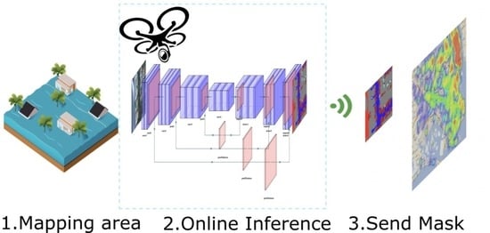
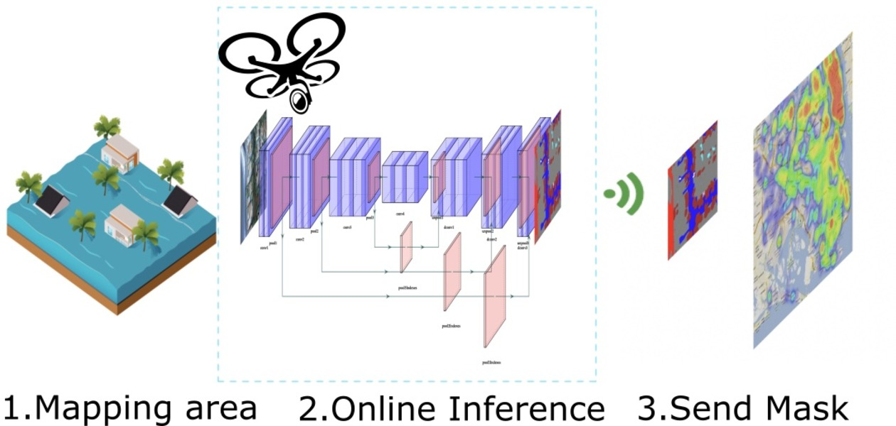
Figure 1 shows an overview of the structure of the proposed solution. Major contributions of this paper are the following:
- 1.
Different state of the art DNN-based deep learning models for image segmentation are analyzed for flooding detection in terms of performance, accuracy, and memory footprint. Particularly, PSPNet, DeepLabV3, and U-Net are under study.
- 2.
Several encoders are also analyzed as they are the main bottleneck for the memory footprint, the disk weight, and the execution time of the inference process. Particularly, we analyze ResNet152, EfficientNet, and MobileNet.
- 3.
The Cartesian product of these neural networks models and encoders are trained to identify flooded areas from aerial images; i.e., nine models in total. A semisupervised training procedure with a pseudolabeling strategy is designed to increase the accuracy in up to 4%.
- 4.
An in-depth performance evaluation of different low-power GPU-based edge computing devices is provided to assess the feasibility of autonomous AI drones in detecting flooding areas.
- 5.
An evaluation in terms of memory, performance, and quality is provided to analyze which of the models and encoders for flood image segmentation is best suited to be run on drones to provide real-time feedback to decision-makers.
The article is structured as follows.
Section 2 introduces the general infrastructure, the main deep learning models targeted, and methods used to deal with aerial images of flooded areas.
Section 3 shows the experimental setup before showing the performance and quality evaluation of our approach. A discussion of the results is then provided in
Section 4. Finally,
Section 5 shows conclusions and directions for future work.
2. Materials and Methods
This section introduces different neural network models that are widely used in detecting flooded areas. These models will be trained in order to obtain the segmentation mask of each image from the drone. The data used and the training procedures carried out are also summarized prior to the evaluation on the drone to be performed in the following section.
2.1. Hardware Environment
The UAV device that supports the segmentation hardware consists of the following components:
DJI F550 frame.
Pixhawk flight controller.
Processing unit.
Marshall Electronics CV503-WP Mini Full HD Camera.
Battery Tattu 9000 mAh 22.2 V 25 C 6S1P Lipo.
3DR GPS receiver.
Sunnysky X2212 motors—980 kv.
APM 433 MHz telemetry.
Taranis X9D controller + X8R receiver.
Table 1 shows the hardware platforms used to perform the experiments below. Particularly, we use a high-performance computing (HPC) computer, called Pedra, as a baseline for our experiments. Then, three GPU-based edge computing devices from the NVIDIA Jetson family (i.e., Jetson nano, Jetson TX2, and Jetson AGX Xavier) are also targeted. Moreover, the software environment is based on gcc v7.4.0, CUDA v10.2 with cuDNN and Python v3.6 with pytorch v1.8.0 built for edge devices, torchvision v0.9.0 built for edge devices, and scikit-learn v0.24.1.
2.2. Dataset
FloodNet [
17] is a set of images captured in the aftermath of Hurricane Harvey, which made a landfall near Texas and Louisiana on August 2017, as a Category 4 hurricane. In it, special emphasis is placed on areas that have been flooded. In particular, it contains UAV images captured during the response phase by emergency personnel. The authors of the dataset obtained the images using small DJI Mavic Pro quadcopters. The images were captured at a height of 60 m with a spatial resolution of 1.5 cm. Currently, it is the only dataset created with images of floods captured from a drone after a catastrophic event, and at an optimal level of detail to train a neural network that must be operational within a UAV.
Floodnet images are labeled at the pixel level, which makes them useful for the semantic segmentation task. FloodNet attempts to perform fine labeling that encompasses situations such as detecting flooded roads and buildings, and distinguishing between natural water and flooded water. Although the dataset approach is broader than image segmentation, in this particular case, we will focus on it, as the training dataset consists of 51 labeled images of flooded areas, 347 labeled images of nonflooded areas, and 1047 unlabeled images on which pseudolabeling tasks are to be performed. Labeled images include the following instances: Building flooded (3248 instances), Building Non flooded (3427 instances), Road flooded (495 instances), Road Non Flooded (2155 instances), Water (1374 instances), Tree (19682 instances), Vehicle (4535 instances), Pool (1141 instances), and Grass (19682 instances).
2.3. Semantic Segmentation for Flooding Detection
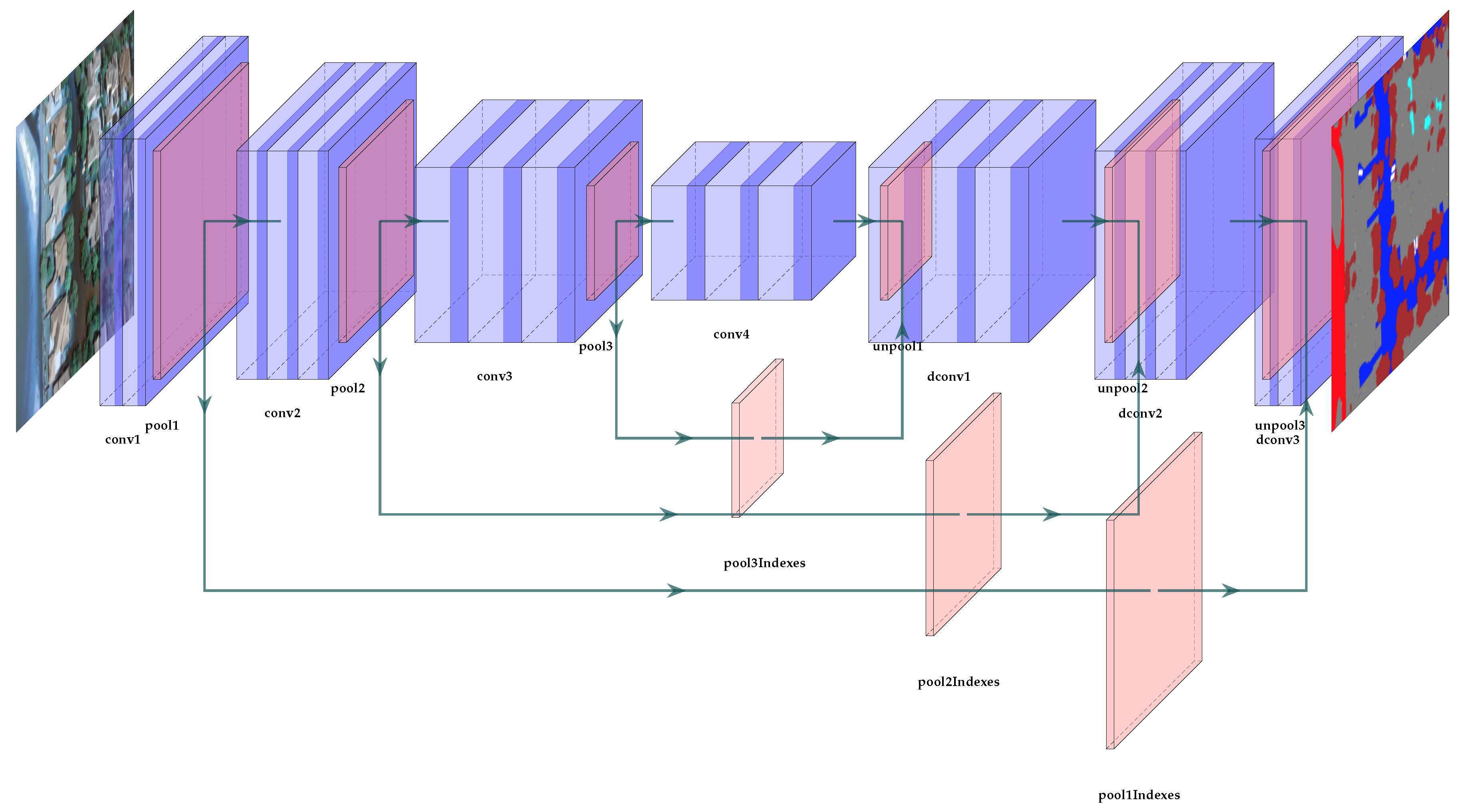
In this study, the experimentation is focused on obtaining the data from the drone for sending. For this task, image segmentation has been considered the technology best suited to the requirements of detecting flooded areas. Semantic segmentation is the technique of classifying parts of an image that belong to the same object class. It is a form of pixel-level prediction where pixels in an image are classified according to a category. An example of this type of network can be seen in
Figure 2, which shows a simple deep convolutional autoencoder where you can see the two main parts of a network dedicated to image segmentation; on the left, the one that tries to capture the visual patterns of the image, and on the right, the one that tries to reconstruct a representation of the detected classes. Notice that image classification merely has to identify what is present in the image, whereas semantic segmentation identifies not only what is present in the image, but also where to find it by signalling all pixels that belong to each characteristic identified. Indeed, since the emergence of deep neural network (DNN), segmentation has made tremendous progress. We refer the reader to [
18,
19,
20] to see a full review of deep learning techniques for image semantic segmentation. Among these techniques, we highlight the following:
PSPNet [21] is a model that uses a pyramid parsing module to exploit the global context information through region-based context aggregation. The combined local and global cues make the final prediction more reliable. Given an input image, PSPNet uses a pretrained CNN with the dilated network strategy to extract the feature map. The final size of the feature map is the same as that of the input image. On top of the map, it uses the pyramid clustering module to gather context information. Using a four-level pyramid, the clustering kernels cover the whole, half, and small portions of the image. They are merged as the global priority and then concatenate the prior with the original feature map in the final part of the decoder. Next, a convolution layer generates the final prediction map.
DeepLabV3 [22] is a semantic segmentation architecture that builds on DeepLabv2 [
23] with the following modifications: in order to deal with the problem of multiscale object segmentation, modules have been designed that use cascaded or parallel Atrous convolution to capture the multiscale context by adopting multiple Atrous rates. Another modification over the previous version is that the Atrous Spatial Pyramid Pooling module [
24] is extended with image-level features that encode the global context, further increasing performance. The last change is that DenseCRF [
25] postprocessing has been dropped.
U-Net [26] uses an encoder–decoder architecture based on a contraction route to capture the context, and a symmetric expansion route to achieve accurate location. It was originally designed for segmenting medical images, and it achieves robust results with a more uniform training set. In recent years, studies have shown that U-Net is also suitable for remote sensing images [
27], and has great potential for improvement.
All the segmentation models mentioned make use of a backbone that is capable of extracting the fine-grained patterns of the image in the form of an encoder of the information. A large part of the trainable parameters of the network come from these blocks, and depending on the type of network chosen for this purpose, the memory footprint, the disk weight, and the execution time of the inference process will be different. For this study, three backbones of different characteristics have been chosen in order to find the best option between inference time and accuracy obtained. These are described below:
ResNet152, or residual networks, is a variant of convolutional neural network that was first introduced by Kaiming et al. [
28]. Its main feature is that it learns the representation functions of the residuals instead of learning the signal representation directly. ResNet introduces the hop connection (or direct access connection) to adjust the input from the previous layer to the next one without any modification of the input, thus allowing a deeper network that is easy to optimize and can gain accuracy by greatly increasing the depth. In this work, the 152-layer version was chosen to perform the encoder task because it obtains better accuracy while maintaining better complexity than other networks, such as Visual Geometry Group (VGG), as the authors explained in their work.
EfficientNet [29] is a type of DNN whose main feature is that it scales uniformly all dimensions of depth, width, and resolution with a set of preset scaling coefficients. It is based on the intuitive concept that the larger the size of the input image, the greater the number of layers and the greater the number of channels the network will need to capture the patterns in the image; this concept has been studied in works such as [
30].
MobileNet [
31] is a convolutional neural network that has been specifically designed to be executed in embedded devices that require solving computer vision tasks. Its architecture is formed by depthwise separable convolutions with the objective of obtaining the lightest possible network and that allows a low latency when executed in devices that have few resources and that do not usually have a graphic accelerator. The complete MobilNetV2 model, which has been used in this work, is formed by the initial convolutional layer of 32 filters and is followed by 19 residual bottleneck layers. The complete model consists of 2 million parameters.
These encoders (i.e., ResNet152, EfficientNet, MobileNet) are trained to embed the information patterns from the aerial images into an input that can be processed by the network in charge of performing the semantic segmentation (i.e., PSPNet, DeepLabV3, U-Net). However, there are certain scenarios, such as the one we are dealing with in this study, where the training dataset for the encoders is very small, i.e., there are a small number of labeled images, and therefore it is difficult to achieve sufficient accuracy to generate an accurate mask of the captured image to serve as input for the image segmentation procedure. Several works proposed the use of transfer learning techniques [
32] to take advantage of the knowledge acquired when solving one problem and apply it to a different but related problem. In transfer learning, neural networks are initialized with weights from a neural network that is already trained (a.k.a., pretrained) using a large, structured, and labeled dataset. This procedure has shown better performance than those trained from scratch on a small dataset [
33].
In this work, we use the ImageNet database for the pretraining of the encoders. ImageNet [
34] is a large visual database designed for visual object recognition. It consists of over 14 million images that have been hand-annotated to indicate which objects appear in them and, in at least one million of these images, bounding boxes are also provided. ImageNet has more than 20,000 categories, each consisting of several hundred images. Imagenet has proven to be optimal for transfer learning exercises, as shown in [
35], where an empirical investigation is provided that studies the importance of the number of images, and the balance between the images of each class and the number of classes.
2.4. Image Preprocessing
To enhance the performance of the network, a series of transformations are performed on the captured image. To facilitate the implementation of these techniques, we have used the albumentations tool [
36], which is a Python library for fast and flexible image augmentations. Albumentations efficiently implements a rich variety of image transform operations that are optimized for performance, and does so while providing a concise, yet powerful, image augmentation interface for different computer vision tasks, including object classification, segmentation, and detection. In particular, the following features are useful for our purposes:
- 1.
Resize: Rescale an image so that the maximum side is equal to maxsize param, maintaining the aspect ratio of the initial image.
- 2.
ShiftScaleRotate: Randomly apply affine transforms: translate, scale, and rotate the input.
- 3.
RGBShift: Randomly shift values for each channel of the input RGB image. In [
37], authors show that images with different wavelengths and RGB channels determine which kind of images with different color spectrum provide better information to generate a better accuracy of our DNN model.
- 4.
RandomBrightnessContrast: Randomly change brightness and contrast of the input image to reduce a model’s sensitivity to color.
- 5.
Normalize: Normalization is achieved through the formula:
This transformation sequence is applied to each of the images after being captured, and before performing the process of obtaining the mask through the neural network. It is an operation that will be performed on each of the edge devices.
2.5. Inference Precision
This section shows the accuracy of the combination models/encoders on the test dataset. First, an evaluation of all of these combinations is provided by training with the dataset described in
Section 2.2. Then, it is analyzed how the accuracy of the models improves with the semisupervised training proposed in
Section 2.6.
The mean intersection-over-union (MIoU) metric was used to measure accuracy. This metric is based on the Jaccard index, which is defined as the ratio of intersection and union area between the predicted segmentation map and the ground truth defined. It was developed by Paul Jaccard, and it is also known as the Jaccard similarity coefficient; specifically, it is a statistic used for gauging the similarity and diversity of sample sets defined as
where
B shows the predicted segmentation maps, and
A represents ground truth.
Based on it, we can calculate IoU, which is a number from 0 to 1 that specifies the amount of overlapping between the predicted and ground truth:
MIoU is defined as the average value of IoU over all label classes. It is generally used to report the performance of segmentation models. It usually ranges between 0 and 1, given as
where
k represents total classes,
is number of true positives, and
and
are false positive and false negatives.
2.6. Semisupervised Training Procedure
As shown in
Section 2.2, the number of labeled instances is very small, consisting of only 398 images. With regard to the number of test images, 47, this value is considered low; therefore, to achieve a correct performance of the network, it is necessary to apply semisupervised learning techniques on the 1047 training images that have not been previously labeled, therefore creating a dataset of 1445 images. Semisupervised learning is a training method that mixes a small amount of labeled data with a large amount of unlabeled data in the training phase. Semisupervised learning stands between unsupervised learning (with no labeled training data) and supervised learning (with only labeled training data). Unlabeled data is only useful if it provides information for label prediction that is either not present in the labeled data, or cannot be obtained from the labeled data alone. The procedure consists of the following steps:
- 1.
Train the model using training labeled data.
- 2.
Infer labels for an unlabeled data.
- 3.
Add confident predicted test observations to our training data.
- 4.
Train the model for a few extra epochs also using the new labeled data.
2.7. Solution Deployment
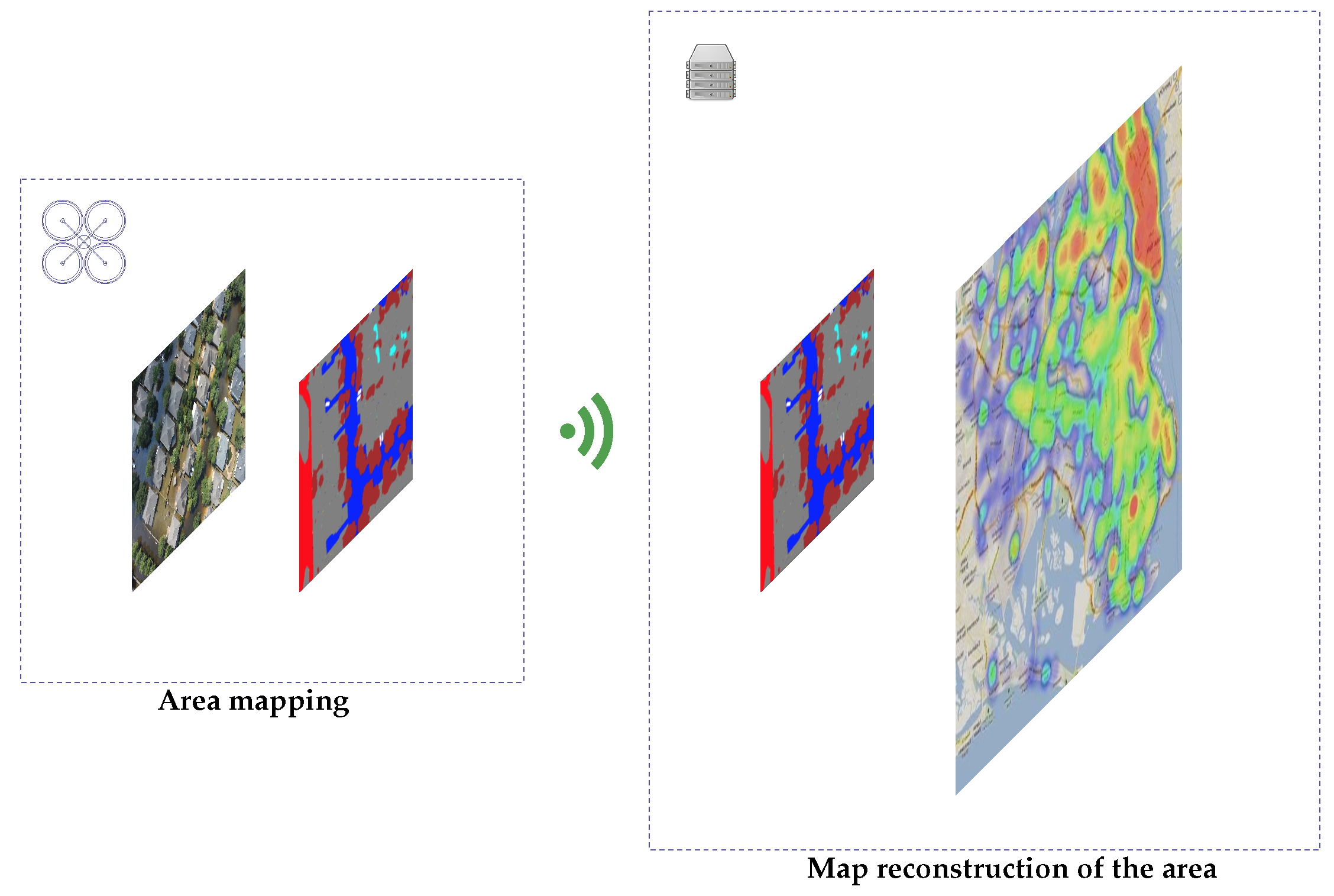
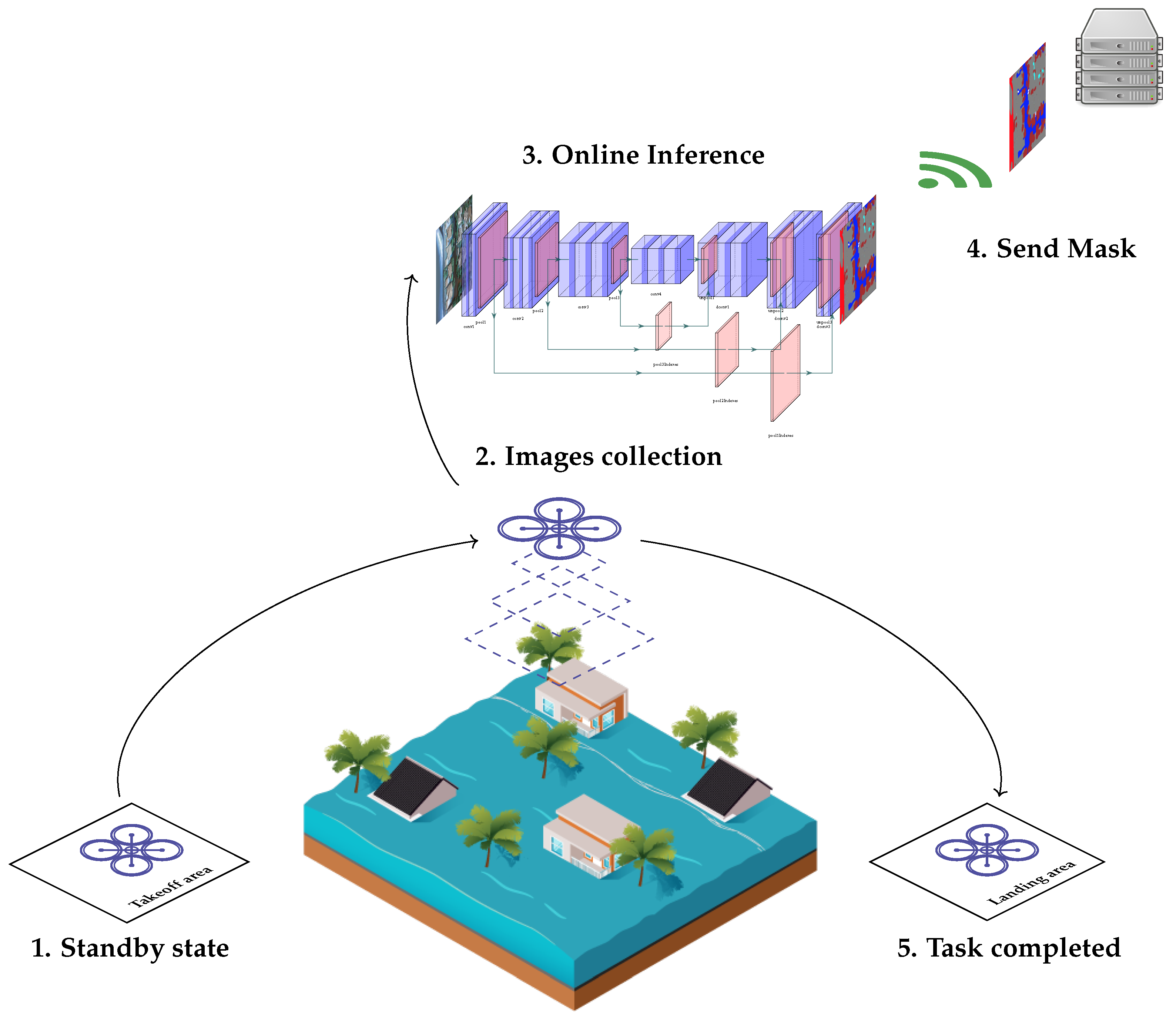
Once the problem has been defined, and the image segmentation proposal enabling a subsequent reconstruction on the server has been proposed as a solution, we now proceed to describe the execution flow that would be carried out in a real natural disaster management scenario.
Figure 3 shows the life cycle of an image collection and processing mission at the edge. The UAVs start from a standby position (step 1) to prepare for takeoff before starting to gather images from the affected area. While the images are being collected (step 2), the deep learning models (step 3) are running to perform a real-time inference of each of the images from the UAV device, resulting in image processing at the edge. In step 4, images are sent to the server. Steps 2–4 are repeated until all the area to be mapped has been imaged, and all the masks are generated. It is noteworthy that, in step 4, only masks are sent to the cloud, which means using only 4 bits per pixel, instead of the 24 bits per pixel that would be sent in the case of using a standard bitmap having 24 bits. Notice that 4 bits per pixel are adopted because they conform to the minimum value required to represent the 10 classes that the system is able to detect, and therefore each pixel of the image can be represented merely by a value between 0 and 9. This significantly reduces the overall bandwidth requirements by a factor of 8, as shown in
Section 3.3.1.
3. Results
This section starts by summarizing the main hardware features of the hardware environment targeted for assessing the deep learning models for image segmentation previously presented. Then, it provides an overview of the dataset used to train and test those models before a performance assessment in terms of quality, execution time, and memory footprint is provided.
This section evaluates the performance (i.e., execution time) and precision of the deep learning architectures previously presented in
Section 2.
3.1. Image Preprocessing Results
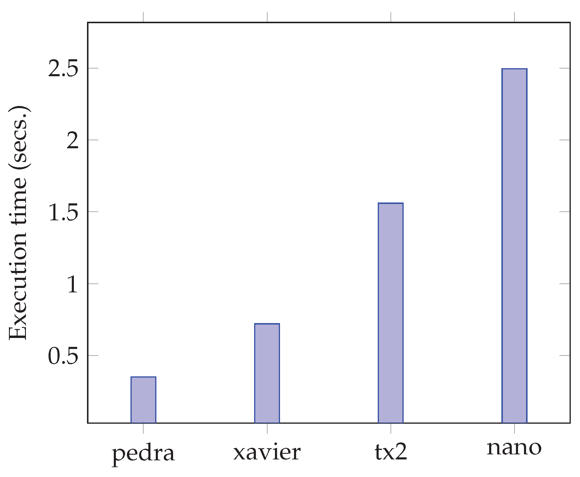
Figure 4 shows the difference in execution time between the different devices. This execution time is added to the mask acquisition time to define the frame rate that can be sent to the server. The HPC server will also be included in each of the time figures in order to have a reference of the inference time that would be required with a non-edge device. The figure shows that the execution times range from 0.35 s on the server hosted in the data center, to 2.49 s on the Jeson Nano device; i.e., a performance loss of up to 7.11× on the edge platform. The difference between these two devices is notorious, and for image processing during the mission, where many images have to be captured within a short timespan, the compartmentalization of this step with the neural network processing will have to be taken into account, being able to execute the processing of the current image on the CPU, while obtaining the mask of the previous image through the neural network using the GPU.
3.2. Inference Precision Results
This section shows the MIoU obtained for each model with each of the chosen encoders.
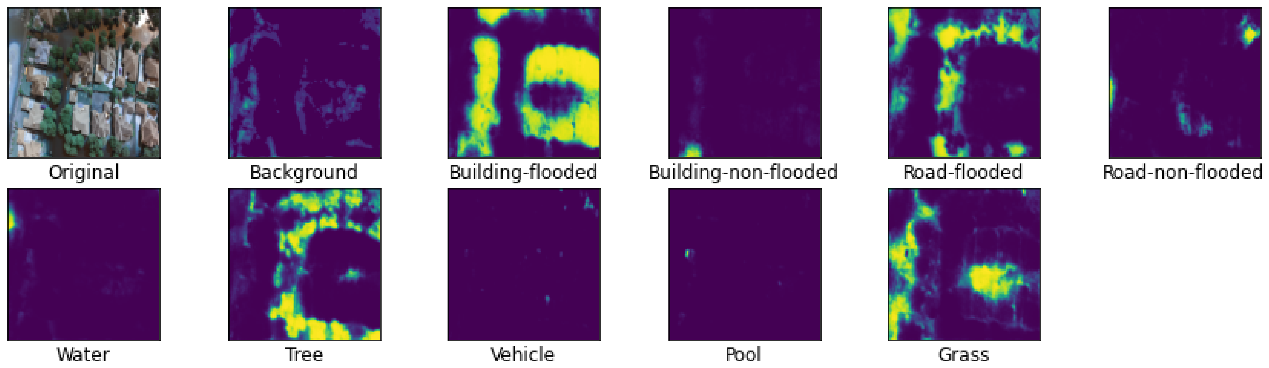
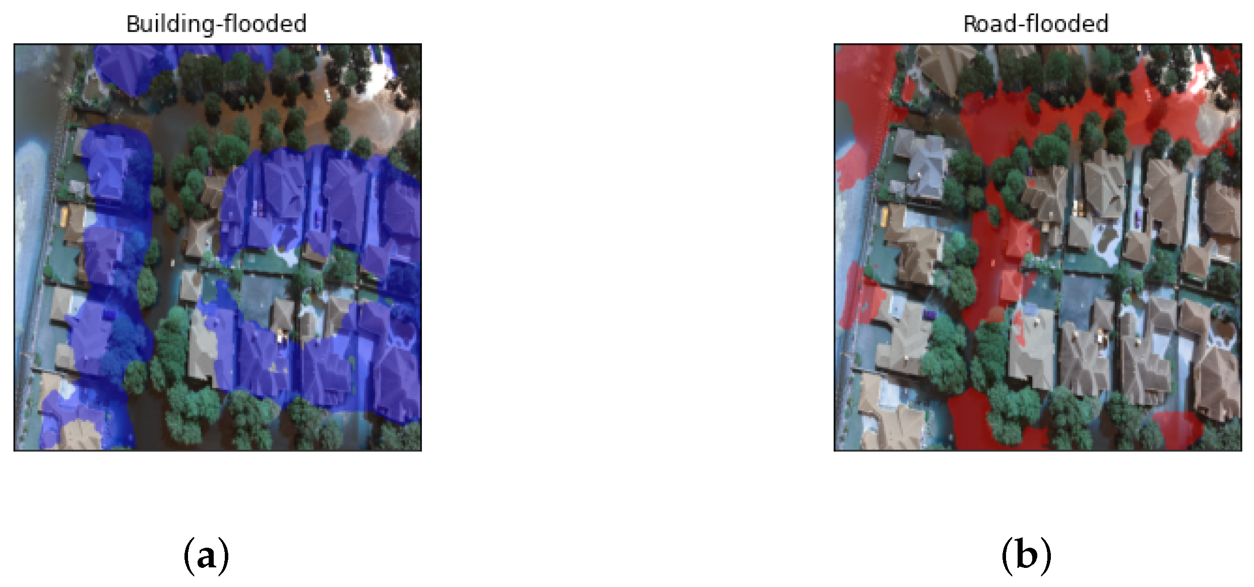
Figure 5 shows the mask generated for each of the 10 classes of the dataset on one of the images of the dataset. For the requirements of this work, only the classes that refer to floods are necessary. Two of these masks are shown in
Figure 6: flooded buildings and flooded roads. Nevertheless, in the training of the network, the IoU of each of the classes was taken into account.
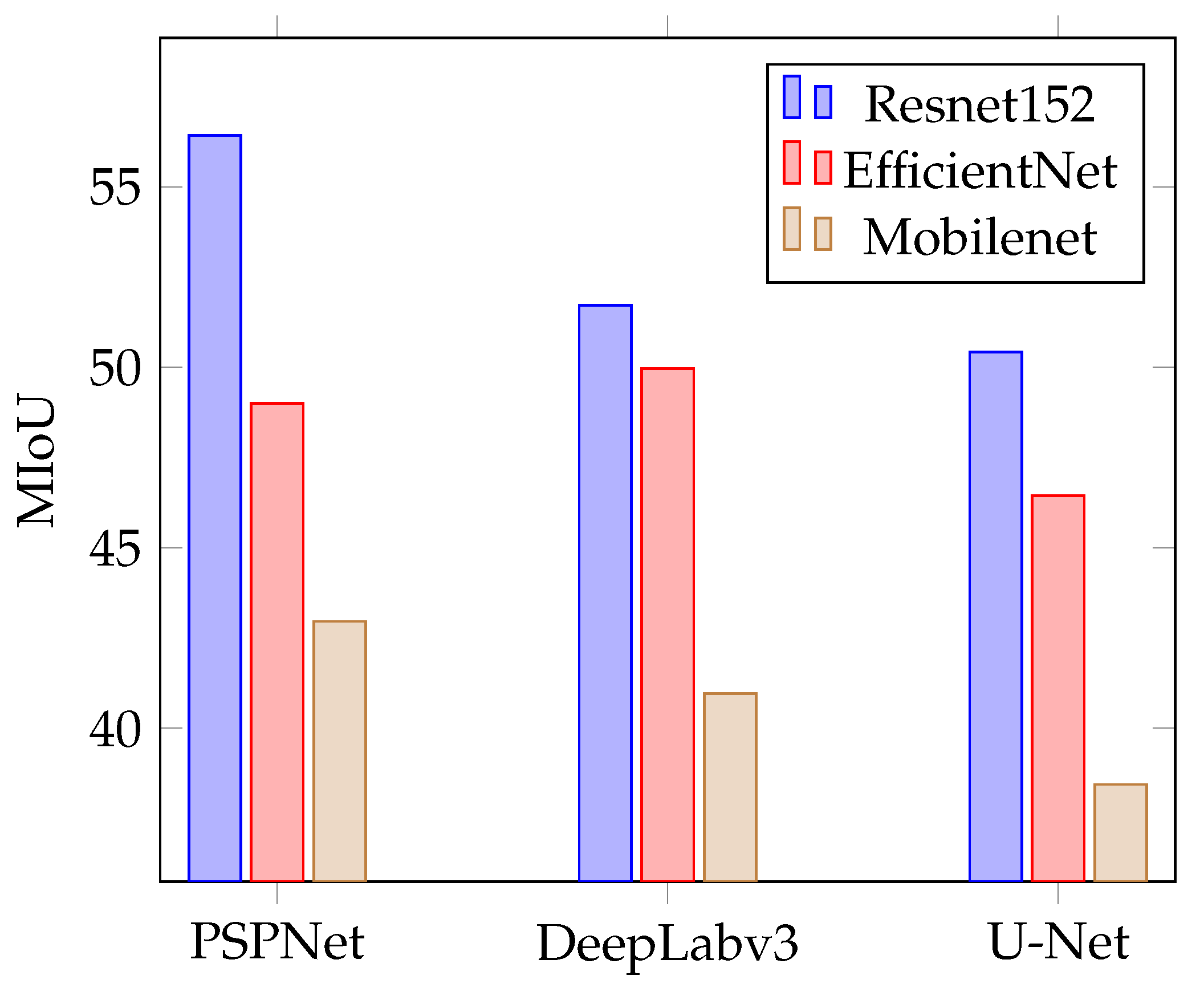
Figure 7 shows the model efficiency based on the MIoU achieved for each combination of neural network model and encoder. For PSPNet training, a constant learning rate of 0.001 for 15 epochs was set; for DeepLabV3, the learning rate was of 0.01 for 10 epochs, while for U-Net it was trained for 15 epochs with a learning rate of 0.001. For the batch size during training, a value of 4 was set for all models when using the RestNet152 encoder, a batch size of 7 for EfficientNet encoders, and 8 for MobileNet encoders. It can be seen that the RestNet152 encoder achieves the best result, with the PSPNet Network having the most significant difference, which increases by more than 5% with respect to EfficientNet. In the DeepLabv3 network, the difference between RestNet and EfficientNet is of 2%, which is not so significant. The MobileNet encoder shows the worst results of all, with a difference of up to 13% compared to the best case.
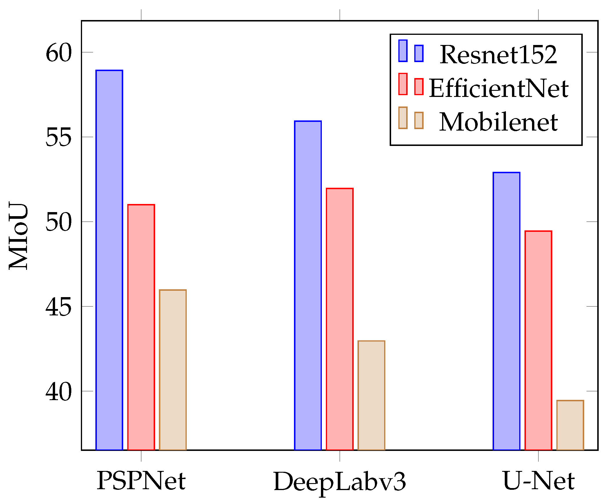
Figure 8 shows the accuracy of the trained models when they are trained using the pseudolabeling technique described in
Section 2.6. For this process, the same parameters of learning rate, number of epochs, and batch size were used as in the previous results shown in
Figure 7.
Figure 8 shows a slight increase in the MIoU of all models: 2% for PSPNet with the ResNet152 encoder, 3% for DeepLabv3; for EfficientNet, the biggest difference is found in the U-Net network with an increase of 4%. The MobileNet encoder obtains almost identical values with U-Net, with a great improvement when it comes to PSPNet. It can be seen that the network that has benefited the most from this type of training is PSPNet. This has to be taken into account when choosing which model to use for the deployment of the solution, since it is possible to add previously unlabeled data to generate soft labels with them, and thus adapt the model to changes that may occur in the area to be mapped.
It is not possible to consider the supremacy of a model over the rest for all the use cases in which image segmentation can be applied, since with another dataset or another task the result may be that DeepLabv3 or U-Net behave better than PSPNet; for this reason it would be necessary to redo the experimentation and perform a reparametrization of the learning rate, optimizer, and other factors that may affect the performance of the network.
3.3. Model Comparative
This section shows a comparison of the three models chosen with their corresponding encoders in terms of size, performance, and inference time for each of the edge computing devices to be embedded in a UAV. The size of a model is represented by the number of trainable parameters of the model. After the training process, these models are usually serialized in a certain standard format to be distributed to different applications, and for different devices. The size of the exported model on disk will be smaller than the size it will occupy in memory and, therefore, these two variables must be taken into account in the study of the space footprint of a model. The size of each encoder used must also be taken into account, and a choice then made based on the size and accuracy of the encoder.
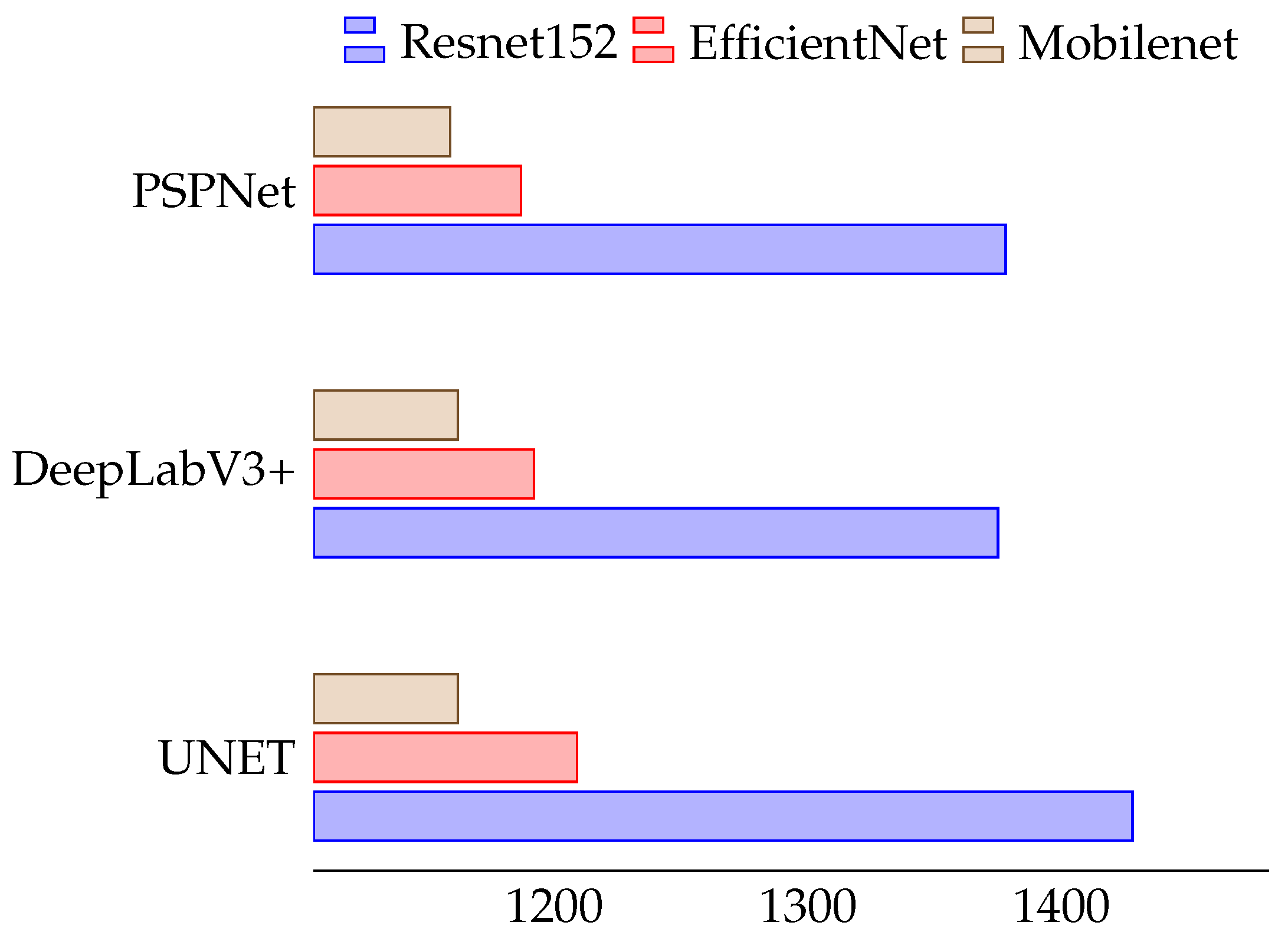
Figure 9 shows a comparison of the disk size (in MB) of each serialized model, and for each of the encoders used in the training phase (i.e., ResNet152, EfficientNet, and MobileNet). It can be seen that, regardless of the network used, ResNet152 has a much higher weight than the rest, the difference between DeepLabV3 and PSPNet being negligible, of 235 MB for DeepLabV3, and of 226 MB for PSPNet. For EfficientNet, both Deeplab3 and PSPNet occupy a space of 50 MB. UNet has a slightly lower value of 46 MB. The MobileNet encoder, together with PSPNet, has the smallest footprint of all combinations, with a value of 9.1 MB, followed by equal values of 17 MB for the two other networks.
Figure 10 shows a comparison (in MB) of the footprint of each model when deserialized in memory. As in
Figure 9, the values of each of the encoders with each of the models are shown. The increase in space required with respect to the serialized model is evident, tripling in all models. These results will have to be taken into account when deploying each of the models on edge devices, especially in the TX2 and Jetson Nano platforms where the GPU memory capacity is very limited.
The inference time, together with the image preprocessing time, is one of the values to be taken into account when deploying the trained model for the inference process. Undoubtedly, a compromise has to be found between the accuracy of the models and the time it will take to obtain the result; i.e., the mask of the image captured by the drone. An elongate inference time to generate the mask would prevent the real-time processing we are looking for to help first responders. Therefore, the ideal scenario would be to process the image and send its mask before the next image is captured. For this reason, a performance evaluation for each model + encoder targeted on each edge computing platform that can be embedded in a UAV was carried out. CPU and GPU processing times were measured to study, in which case it is necessary to install the latter, and in which case a single CPU would be enough, thus saving both weight and energy, which would reduce both the weight and the power consumption of the UAV. The HPC server is included in each of the time figures in order to have a reference of the inference time that would be required with a non-edge device.
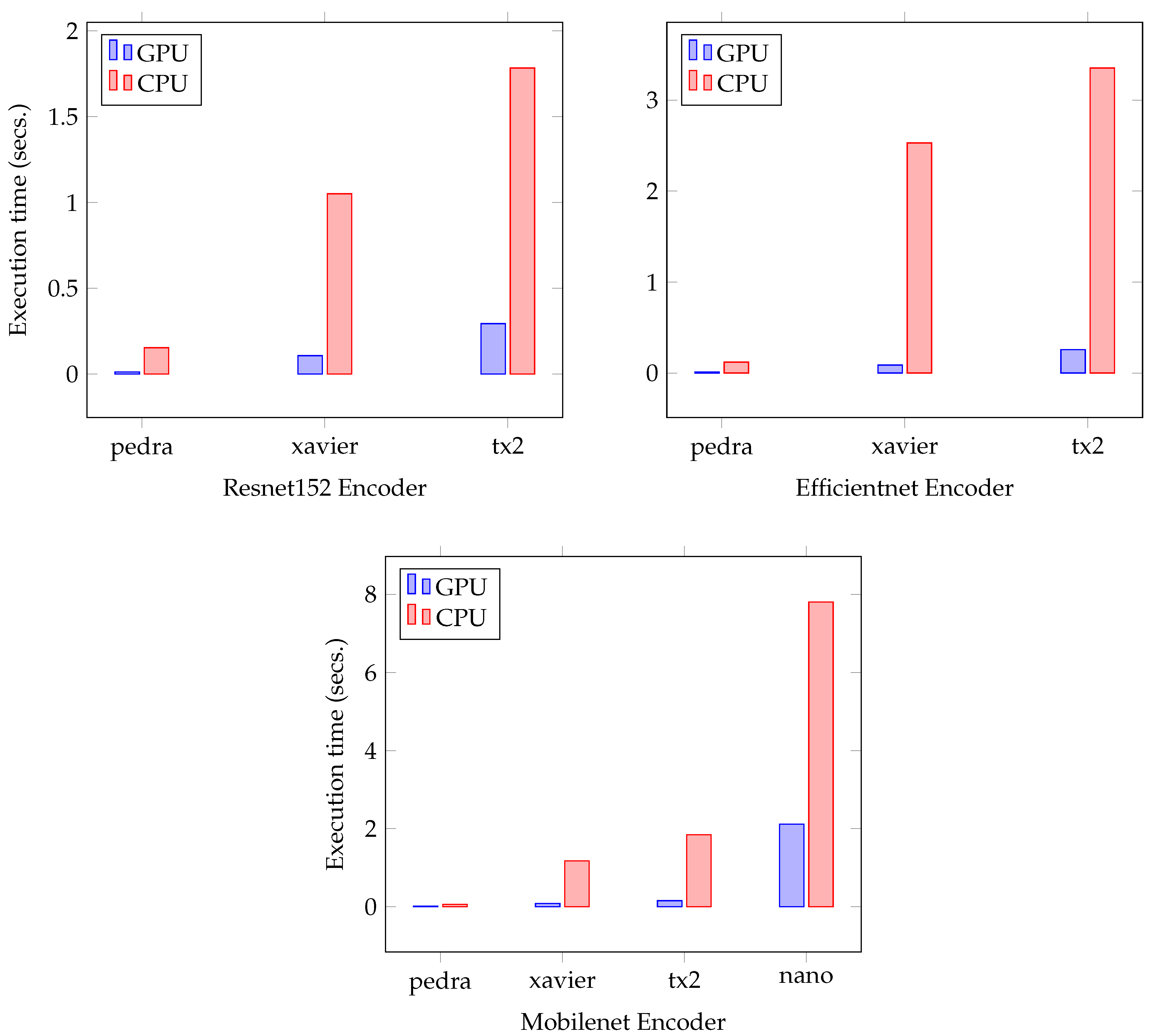
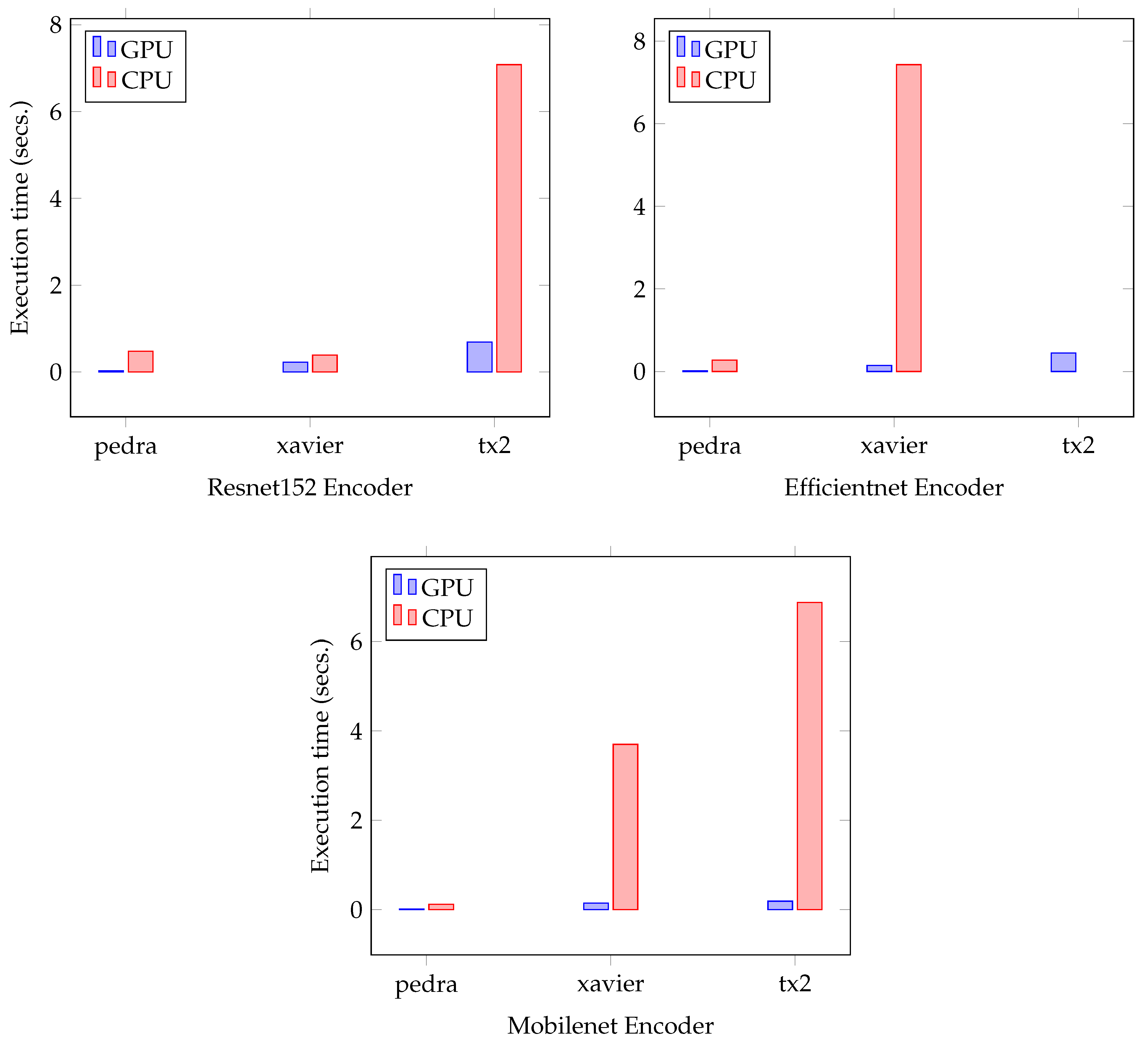
Figure 11 shows three bar charts, all corresponding to the PSPNet network with each of the given encoders. For each of the bar charts, the execution time on GPU and CPU is shown. The ResNet encoder could only be executed on the Xavier and TX2 devices, the latter doubling the Xavier platform in both GPU and CPU time. The Jetson Nano device could not finish the inference process, and therefore some simplifications would have to be made on it in order to run it. PSPNet, together with EfficientNet, could not be run on the Jetson Nano platform either, and both the AGX Xavier and TX2 show similar inference times. PSPNet-MobileNet could be executed on the Jetson Nano device, this being the only encoder out of the three with which we have experimented that could be hosted without problems, although the execution time is several orders of magnitude higher than that of TX2 and Xavier which, as with EfficientNet, have very similar times, to the detriment of TX2.
Figure 12 follows the same structure as
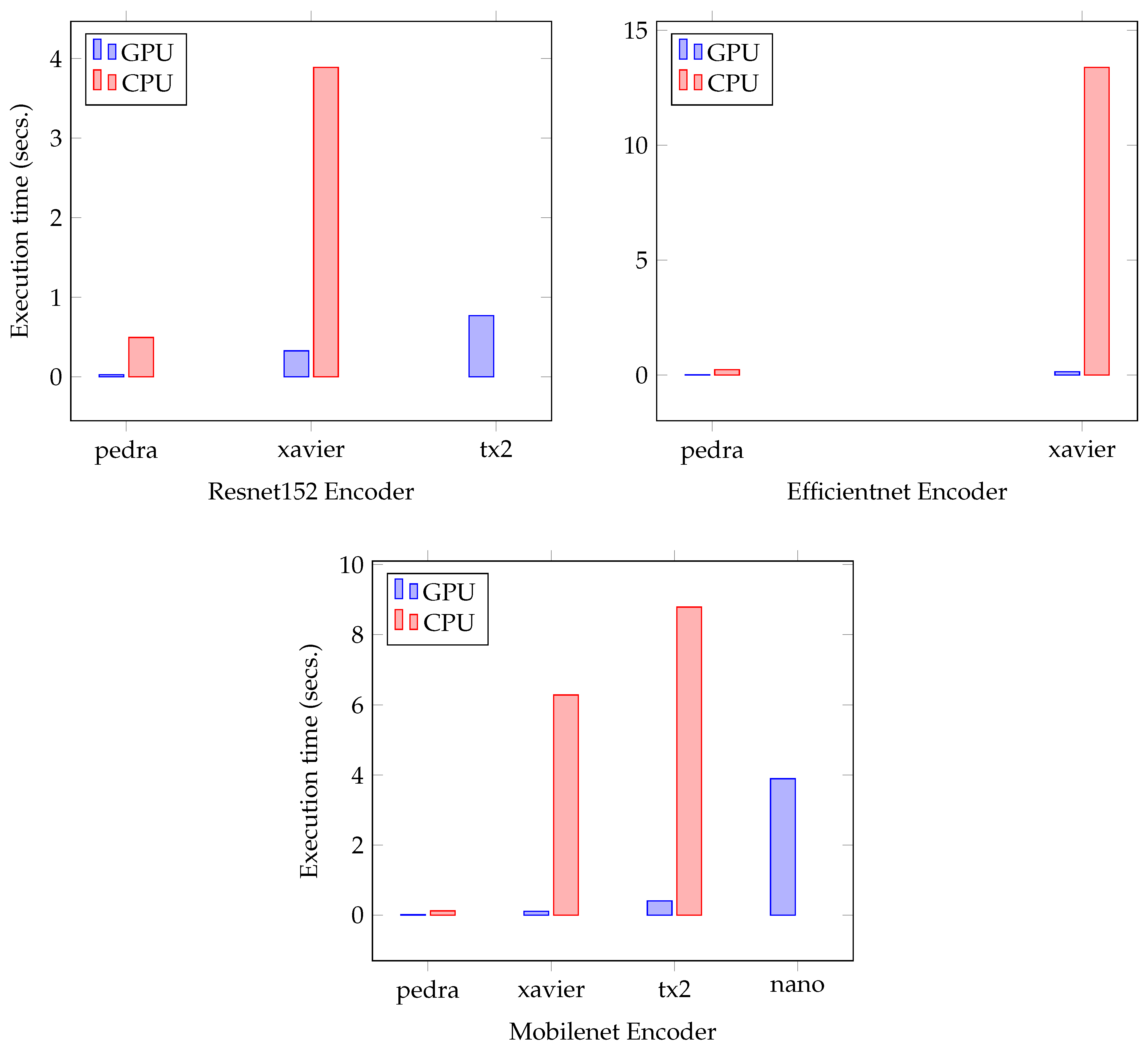
Figure 11, but showing the UNET execution times with all encoders. This network is the one that shows the most limitations in terms of execution, where only the MobileNet encoder was able to be executed in all the devices, and where the execution times are higher than in the other two models. In the first graph, with ResNet, the execution in the Jetson Nano platform was not possible, and in TX2 only when using the GPU, and with a time overhead close to the second. In the EfficientNet encoder, it was only possible to perform the execution in the Xavier platform, with a remarkable CPU time of 14 s per image. MobileNet was executed on all devices using GPU, while the Jetson Nano device could not be executed on CPU.
Figure 13 follows the same structure as in
Figure 11, but showing the DeeplabV3 execution times with all encoders. The big difference is that this model could not be run on the Jetson Nano device with any encoder. In ResNet152 it can be seen how, in the TX2 platform in the CPU, the time is very high with respect to Xavier, achieving a GPU time of less than 1 s. In EfficientNet, the execution times are significantly higher than in ResNet152, and it was not possible to perform the execution of the TX2 platform in the CPU due to lack of memory. Using MobileNet, the fastest execution times are achieved within the TX2 device, but not for Xavier.
3.3.1. Data Compression
Following the image classification procedure described before, the next step consists of sending an alert to the control station located in the cloud with the frame, and the meta-information that details the coordinates marked as positive for the emergency team to evaluate them. We show a comparison between sending the raw information and the mask resulting from the network processing. Notice that by just sending the mask, we are able to save bandwidth.
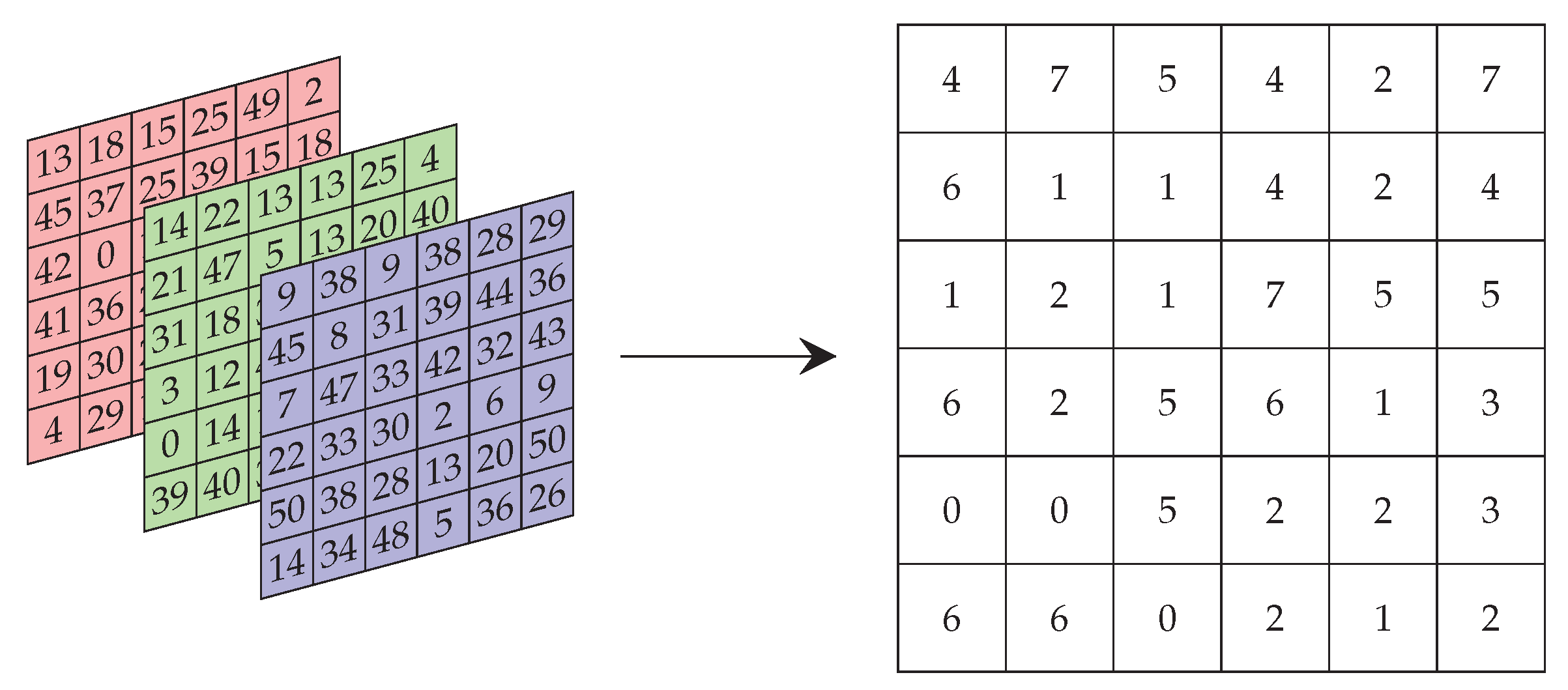
Figure 14 shows the information compression achieved by sending the mask to the server from the UAV. If the complete image was used, the values represented over three channels would be sent with values ranging from 0–255. However, to store the segmentation information found according to the target classes, only one channel and one value for each of the classes is needed. In this case, the dataset has a maximum of 10 classes, and so only 4 bits would be needed for each pixel represented, in contrast to the 8 bits per pixel required when sending the original image.
This compression represents a saving in the bandwidth to be transmitted, which would affect both the consumption and the speed of sending information to the server. In particular, the original image sized 4000 × 3000, which occupies 5.488 MB, would in turn generate a mask of 910 KB, which would represent a saving of 83.42% of the information to be transmitted. This would not be enough if we were looking for a detailed representation of the information. Nevertheless, in this work, we are merely aiming at sending enough information to be able to reconstruct the scene on which the tracking operation is being performed, this being the information collected by the semantic classification of the entities of the captured image.
4. Discussion
In the experimentation carried out in the previous section, we extracted the data to be taken into account when implementing an area monitoring system using semantic segmentation perform from a resource-constrained device such as a drone. In this section, and based on the results obtained, we discuss the most solid proposal to be deployed.
This study used an input-ready dataset, so far the best suited to the task at hand, using semisupervised learning techniques, which is an obvious disadvantage compared to a rich dataset with each instance correctly labeled in all photos; this reveals that more work needs to be carried out on collecting and labeling flooding datasets derived from UAVs. A positive observation regarding the results obtained using such a small dataset is that, using semisupervised learning techniques, it would be possible to deploy the solution in areas where the geography and architecture are different from the training dataset, and a process of image collection and labeling is required. By obtaining a small sample, and with a training process of less than 10 epochs, a functional model to run on the UAV would be available.
In terms of accuracy based on the Floodnet validation dataset, we can estimate that the PSPNet network, together with a Resnet152 encoder pretrained on ImageNet, and further trained in a semisupervised way using soft labels, is the combination that will allow a more accurate server reconstruction of the mapped area, achieving 56% of MIoU. This is a valid result to solve the problem of obtaining a mask of flooded areas on roads, buildings, and places near river or sea beds, as it would allow differentiating natural water masses from those that have flooded areas, and where water is not expected.
Figure 5 and
Figure 6 show an example of the pixel-level segmentation of each of the classes detected. This information is the main component in the server reconstruction of the monitored area. The main issue of using this proposal is its memory size limitation, as it is the second largest model in terms of memory footprint, and hence cannot run on a Jetson Nano device, which is the most suitable device to be installed on a UAV due to its weight and dimensions. Another advantage of selecting these parameters is their speed, as they would be among the fastest of all those studied; if we wanted to use them, we would obtain a speed of less than half a second on a TX2 device using the GPU. On the opposite side, UNet has been the most problematic model in terms of execution and adaptation to the different edge devices, and some of its parameterizations, for example using Efficientnet, do not allow its execution neither in TX2 nor in Nano, the two lightest devices, and therefore is more susceptible to be assembled in a UAV.
If the weight and power limitations are sufficient to install a Xavier device, PSP-Resnet152 would be the best option. Otherwise, and if we were looking for the most efficient solution in these two parameters, we would have to use a Jetson Nano, and our software combination would be limited to the PSPNet-MobileNet and Unet-MobileNet models (GPU restricted), with an MiOU of 45.9 and 39.4, respectively, and a GPU execution time of 2 s and 8 s CPU in PSPNet, against 4 s in Unet GPU. Therefore, PSP-MobileNet would be the best choice for the Jetson Nano platform. In case a weight margin could be obtained in the processor, and the weight of the UAV is not excessive, it would be convenient to install a TX2 device, as for 24 grams and a little more power consumption, the best combination would be achieved, which would mean an improvement of 13% in accuracy, and a reduction of execution time of 1.7 s if the GPU is used, and of 6 s if CPU power is used instead. Therefore, a good configuration, offering an adequate trade-off between accuracy, execution time, weight, and power of the drone, could be the TX2 platform as an inference hardware device where a PSPNet network would be deployed with a ResNet152 encoder pretrained with ImageNet.
The frame-sending interval (process that starts when a new image is obtained, and that ends with the sending of the mask obtained to the server, without taking into account the network speed and latency of the same), that could be achieved with the best solution would be of 1.5 s of image preprocessing time, plus 0.29 s of GPU inference, so it would be 2 s using GPU (0.5 Hz) and 3.3 s in the case of using only the CPU (0.3 Hz). In addition, as shown in the compression section, the bandwidth of sending the information from the drone will be significantly reduced when generating the mask on the edge, and that can save network resources and lower battery consumption.
5. Conclusions
UAVs have the potential to play a “key role” in mitigating the consequences of climate change. However, both hardware and software solutions are needed to make these devices truly crucial players in these tasks. AI and edge computing are undoubtedly a winning combination by enabling to transform autonomous drones into useful tools in various emergency situations. In this work, an AI-based pipeline was proposed for execution on edge computing platforms to enable efficient processing of natural disaster images captured by UAVs.
Our results reveal that the use of neural networks designed for real-time image segmentation from drones can be a viable solution as long as the drone is equipped with an edge computing device endowed with GPUs. The benefit of merely sending the result mask instead of the raw image, which is made possible by performing image processing at the same location where the image is captured, reduces the required network traffic by several orders of magnitude. It is worth mentioning that the computational load differences between edge and cloud platforms remain large, with speedup factors in the range of 2.8×–22.17×. Yet, the development of efficient platforms for the execution of specific workloads, such as deep learning, shows a roadmap that enables the development of applications for relevant autonomous and intelligent systems, such as the one proposed here.
We are certain that autonomous UAV technology can be an important factor in the fight against climate change. This study has shown how, with a small dataset correctly labeled and the right model, a real-time segmentation system can be embedded in a UAV, bringing the main computational work closer to the device in charge of processing the information to make an offline inference and send the digested data. However, there is still a lot of work to be undertaken from several points of view. In terms of communication, extending the results of this article to a swarm of drones can provide a greater coverage of the area to be surveyed, something very necessary in this type of natural catastrophe. Additionally, it becomes necessary to increase the performance of IA models by providing new datasets, as well as studying in more depth the representation part of the semantic segmentation result obtained by the network on a map of the area where images have been captured, so as to provide greater insights.
Author Contributions
Conceptualization, J.M.C. and C.T.C.; methodology, J.M.C.; software, D.H.; validation, J.M.C.; formal analysis, D.H. and J.M.C.; data curation, D.H.; writing—original draft preparation, D.H.; writing—review and editing, J.M.C., C.T.C. and J.-C.C.; supervision, J.M.C. and J.-C.C.; project administration, J.M.C., C.T.C. and J.-C.C.; funding acquisition, J.M.C., C.T.C. and J.-C.C. All authors have read and agreed to the published version of the manuscript.
Funding
This work is derived from R&D projects RTI2018-096384-B-I00 and RTC2019-007159-5, as well as the Ramon y Cajal Grant RYC2018-025580-I, funded by MCIN/AEI/10.13039/501100011033, “ FSE invest in your future” and “ERDF A way of making Europe”, and by the “Conselleria de Educación, Investigación, Cultura y Deporte, Direcció General de Ciéncia i Investigació, Proyectos AICO/2020”, Spain, under Grant AICO/2020/302.
Conflicts of Interest
The authors declare no conflict of interest.
References
- Austin, R. Unmanned Aircraft Systems: UAVS Design, Development and Deployment; John Wiley & Sons: Hoboken, NJ, USA, 2011; Volume 54. [Google Scholar]
- Shakhatreh, H.; Sawalmeh, A.H.; Al-Fuqaha, A.; Dou, Z.; Almaita, E.; Khalil, I.; Othman, N.S.; Khreishah, A.; Guizani, M. Unmanned aerial vehicles (UAVs): A survey on civil applications and key research challenges. IEEE Access 2019, 7, 48572–48634. [Google Scholar] [CrossRef]
- Rohman, B.P.; Andra, M.B.; Putra, H.F.; Fandiantoro, D.H.; Nishimoto, M. Multisensory surveillance drone for survivor detection and geolocalization in complex post-disaster environment. In Proceedings of the IGARSS 2019—2019 IEEE International Geoscience and Remote Sensing Symposium, Yokohama, Japan, 28 July–2 August 2019; pp. 9368–9371. [Google Scholar]
- Hagen, N.A.; Kudenov, M.W. Review of snapshot spectral imaging technologies. Opt. Eng. 2013, 52, 090901. [Google Scholar] [CrossRef] [Green Version]
- Wang, Y.W.; Reder, N.P.; Kang, S.; Glaser, A.K.; Liu, J.T. Multiplexed optical imaging of tumor-directed nanoparticles: A review of imaging systems and approaches. Nanotheranostics 2017, 1, 369. [Google Scholar] [CrossRef]
- Geelen, B.; Tack, N.; Lambrechts, A. A snapshot multispectral imager with integrated tiled filters and optical duplication. In Advanced Fabrication Technologies for Micro/Nano Optics and Photonics VI; International Society for Optics and Photonics: San Francisco, CA, USA, 18 March 2013; Volume 8613, p. 861314. [Google Scholar]
- Khan, W.Z.; Ahmed, E.; Hakak, S.; Yaqoob, I.; Ahmed, A. Edge computing: A survey. Future Gener. Comput. Syst. 2019, 97, 219–235. [Google Scholar] [CrossRef]
- Guo, D.; Gu, S.; Xie, J.; Luo, L.; Luo, X.; Chen, Y. A Mobile-assisted Edge Computing Framework for Emerging IoT Applications. ACM Trans. Sens. Netw. (TOSN) 2021, 17, 1–24. [Google Scholar] [CrossRef]
- Balemans, D.; Casteels, W.; Vanneste, S.; de Hoog, J.; Mercelis, S.; Hellinckx, P. Resource efficient sensor fusion by knowledge-based network pruning. Internet Things 2020, 11, 100231. [Google Scholar] [CrossRef]
- Zhou, S.; Wang, Y.; Chen, D.; Chen, J.; Wang, X.; Wang, C.; Bu, J. Distilling Holistic Knowledge with Graph Neural Networks. In Proceedings of the IEEE/CVF International Conference on Computer Vision, Montreal, QC, Canada, 10–17 October 2021; pp. 10387–10396. [Google Scholar]
- Balamuralidhar, N.; Tilon, S.; Nex, F. MultEYE: Monitoring System for Real-Time Vehicle Detection, Tracking and Speed Estimation from UAV Imagery on Edge-Computing Platforms. Remote Sens. 2021, 13, 573. [Google Scholar] [CrossRef]
- Tang, F.; Gao, W.; Zhan, J.; Lan, C.; Wen, X.; Wang, L.; Luo, C.; Cao, Z.; Xiong, X.; Jiang, Z.; et al. AIBench training: Balanced industry-standard AI training benchmarking. In Proceedings of the 2021 IEEE International Symposium on Performance Analysis of Systems and Software (ISPASS), Stony Brook, NY, USA, 28–30 March 2021; pp. 24–35. [Google Scholar]
- Nijhawan, R.; Rishi, M.; Tiwari, A.; Dua, R. A Novel Deep Learning Framework Approach for Natural Calamities Detection. In Information and Communication Technology for Competitive Strategies; Springer: Berlin, Germany, 2019; pp. 561–569. [Google Scholar]
- Gebrehiwot, A.; Hashemi-Beni, L.; Thompson, G.; Kordjamshidi, P.; Langan, T.E. Deep convolutional neural network for flood extent mapping using unmanned aerial vehicles data. Sensors 2019, 19, 1486. [Google Scholar] [CrossRef] [Green Version]
- Singh, A.; Singh, K.K. Satellite image classification using Genetic Algorithm trained radial basis function neural network, application to the detection of flooded areas. J. Vis. Commun. Image Represent. 2017, 42, 173–182. [Google Scholar] [CrossRef]
- Hernández, D.; Cano, J.C.; Silla, F.; Calafate, C.T.; Cecilia, J.M. AI-enabled autonomous drones for fast climate change crisis assessment. IEEE Internet Things J. 2021. early access. [Google Scholar] [CrossRef]
- Rahnemoonfar, M.; Chowdhury, T.; Sarkar, A.; Varshney, D.; Yari, M.; Murphy, R.R. FloodNet: A High Resolution Aerial Imagery Dataset for Post Flood Scene Understanding. IEEE Access 2021, 9, 89644–89654. [Google Scholar] [CrossRef]
- Garcia-Garcia, A.; Orts-Escolano, S.; Oprea, S.; Villena-Martinez, V.; Martinez-Gonzalez, P.; Garcia-Rodriguez, J. A survey on deep learning techniques for image and video semantic segmentation. Appl. Soft Comput. 2018, 70, 41–65. [Google Scholar] [CrossRef]
- Lateef, F.; Ruichek, Y. Survey on semantic segmentation using deep learning techniques. Neurocomputing 2019, 338, 321–348. [Google Scholar] [CrossRef]
- Minaee, S.; Boykov, Y.Y.; Porikli, F.; Plaza, A.J.; Kehtarnavaz, N.; Terzopoulos, D. Image segmentation using deep learning: A survey. IEEE Trans. Pattern Anal. Mach. Intell. 2021. early access. [Google Scholar] [CrossRef]
- Zhao, H.; Shi, J.; Qi, X.; Wang, X.; Jia, J. Pyramid Scene Parsing Network. In Proceedings of the IEEE Conference on Computer Vision and Pattern Recognition (CVPR), Honolulu, HI, USA, 21–26 July 2017. [Google Scholar]
- Chen, L.C.; Papandreou, G.; Schroff, F.; Adam, H. Rethinking atrous convolution for semantic image segmentation. arXiv 2017, arXiv:1706.05587. [Google Scholar]
- Chen, L.C.; Papandreou, G.; Kokkinos, I.; Murphy, K.; Yuille, A.L. Deeplab: Semantic image segmentation with deep convolutional nets, atrous convolution, and fully connected crfs. IEEE Trans. Pattern Anal. Mach. Intell. 2017, 40, 834–848. [Google Scholar] [CrossRef]
- He, K.; Zhang, X.; Ren, S.; Sun, J. Spatial pyramid pooling in deep convolutional networks for visual recognition. IEEE Trans. Pattern Anal. Mach. Intell. 2015, 37, 1904–1916. [Google Scholar] [CrossRef] [Green Version]
- Liu, F.; Lin, G.; Shen, C. CRF learning with CNN features for image segmentation. Pattern Recognit. 2015, 48, 2983–2992. [Google Scholar] [CrossRef] [Green Version]
- Ronneberger, O.; Fischer, P.; Brox, T. U-net: Convolutional networks for biomedical image segmentation. In Proceedings of the International Conference on Medical Image Computing and Computer-Assisted Intervention, Munich, Germany, 5–9 October 2015; pp. 234–241. [Google Scholar]
- Huang, B.; Lu, K.; Audebert, N.; Khalel, A.; Tarabalka, Y.; Malof, J.; Boulch, A.; Le Saux, B.; Collins, L.; Bradbury, K.; et al. Large-scale semantic classification: Outcome of the first year of Inria aerial image labeling benchmark. In Proceedings of the IGARSS 2018-IEEE International Geoscience and Remote Sensing Symposium, Valencia, Spain, 22–27 July 2018; pp. 1–4. [Google Scholar]
- He, K.; Zhang, X.; Ren, S.; Sun, J. Deep residual learning for image recognition. In Proceedings of the IEEE Conference on Computer Vision and Pattern Recognition, Las Vegas, NV, USA, 27–30 June 2016; pp. 770–778. [Google Scholar]
- Tan, M.; Le, Q. Efficientnet: Rethinking model scaling for convolutional neural networks. In Proceedings of the International Conference on Machine Learning, PMLR, Long Beach, CA, USA, 9–15 June 2019; pp. 6105–6114. [Google Scholar]
- Lu, Z.; Pu, H.; Wang, F.; Hu, Z.; Wang, L. The expressive power of neural networks: A view from the width. In Proceedings of the 31st International Conference on Neural Information Processing Systems, Long Beach, CA, USA, 4–9 December 2017; pp. 6232–6240. [Google Scholar]
- Sandler, M.; Howard, A.; Zhu, M.; Zhmoginov, A.; Chen, L.C. Mobilenetv2: Inverted residuals and linear bottlenecks. In Proceedings of the IEEE Conference on Computer Vision and Pattern Recognition, Salt Lake City, UT, USA, 18–23 June 2018; pp. 4510–4520. [Google Scholar]
- Tan, C.; Sun, F.; Kong, T.; Zhang, W.; Yang, C.; Liu, C. A survey on deep transfer learning. In Proceedings of the International Conference on Artificial Neural Networks, Rhodes, Greece, 4–7 October 2018; pp. 270–279. [Google Scholar]
- Van Opbroek, A.; Achterberg, H.C.; Vernooij, M.W.; De Bruijne, M. Transfer learning for image segmentation by combining image weighting and kernel learning. IEEE Trans. Med Imaging 2018, 38, 213–224. [Google Scholar] [CrossRef] [Green Version]
- Deng, J.; Dong, W.; Socher, R.; Li, L.J.; Li, K.; Fei-Fei, L. Imagenet: A large-scale hierarchical image database. In Proceedings of the 2009 IEEE Conference on Computer Vision and Pattern Recognition, Miami, FL, USA, 20–25 June 2009; pp. 248–255. [Google Scholar]
- Huh, M.; Agrawal, P.; Efros, A.A. What makes ImageNet good for transfer learning? arXiv 2016, arXiv:1608.08614. [Google Scholar]
- Buslaev, A.; Iglovikov, V.I.; Khvedchenya, E.; Parinov, A.; Druzhinin, M.; Kalinin, A.A. Albumentations: Fast and flexible image augmentations. Information 2020, 11, 125. [Google Scholar] [CrossRef] [Green Version]
- Fuentes, A.; Im, D.; Yoon, S.; Park, D. Spectral Analysis of CNN for Tomato Disease Identification. In International Conference on Artificial Intelligence and Soft Computing; Springer: Cham, Switzerland, 2017; pp. 40–51. [Google Scholar] [CrossRef]
| Publisher’s Note: MDPI stays neutral with regard to jurisdictional claims in published maps and institutional affiliations. |
© 2022 by the authors. Licensee MDPI, Basel, Switzerland. This article is an open access article distributed under the terms and conditions of the Creative Commons Attribution (CC BY) license (https://creativecommons.org/licenses/by/4.0/).


