Article

UAV Oblique Imagery with an Adaptive Micro-Terrain Model for Estimation of Leaf Area Index and Height of Maize Canopy from 3D Point Clouds

by
Minhui Li
1,2,
Redmond R. Shamshiri
1,2,*,
Michael Schirrmann
2,
Cornelia Weltzien
1,2,
Sanaz Shafian
3 and
Morten Stigaard Laursen
4
1
Technische Universität Berlin, Straße des 17 Juni 144, 10623 Berlin, Germany
2
Leibniz Institute for Agricultural Engineering and Bioeconomy (ATB), Max-Eyth-Allee 100, 14469 Potsdam, Germany
3
School of Plant and Environmental Sciences, Virginia Polytechnic Institute and State University, Blacksburg, VA 24061-0306, USA
4
Department of Engineering, Aarhus University, Finlandsgade 22, 8200 Aarhus, Denmark
*
Author to whom correspondence should be addressed.
Submission received: 22 November 2021 / Revised: 21 January 2022 / Accepted: 21 January 2022 / Published: 26 January 2022
(This article belongs to the Special Issue 2D and 3D Mapping with UAV Data)

Abstract

:
Leaf area index (LAI) and height are two critical measures of maize crops that are used in ecophysiological and morphological studies for growth evaluation, health assessment, and yield prediction. However, mapping spatial and temporal variability of LAI in fields using handheld tools and traditional techniques is a tedious and costly pointwise operation that provides information only within limited areas. The objective of this study was to evaluate the reliability of mapping LAI and height of maize canopy from 3D point clouds generated from UAV oblique imagery with the adaptive micro-terrain model. The experiment was carried out in a field planted with three cultivars having different canopy shapes and four replicates covering a total area of 48 × 36 m. RGB images in nadir and oblique view were acquired from the maize field at six different time slots during the growing season. Images were processed by Agisoft Metashape to generate 3D point clouds using the structure from motion method and were later processed by MATLAB to obtain clean canopy structure, including height and density. The LAI was estimated by a multivariate linear regression model using crop canopy descriptors derived from the 3D point cloud, which account for height and leaf density distribution along the canopy height. A simulation analysis based on the Sine function effectively demonstrated the micro-terrain model from point clouds. For the ground truth data, a randomized block design with 24 sample areas was used to manually measure LAI, height, N-pen data, and yield during the growing season. It was found that canopy height data from the 3D point clouds has a relatively strong correlation (R2 = 0.89, 0.86, 0.78) with the manual measurement for three cultivars with CH90. The proposed methodology allows a cost-effective high-resolution mapping of in-field LAI index extraction through UAV 3D data to be used as an alternative to the conventional LAI assessments even in inaccessible regions.

1. Introduction

Leaf area index (LAI) is an important ecophysiological parameter for farmers and scientists for evaluating the health and growth of plants over time. It is defined as the ratio of the leaf surface area to the unit ground cover [1]; it describes leaf gas exchange and is used as an indication of the potential for growth development and yield. It is widely employed in crop growth models for optimizing management decisions in order to respond to field uncertainties, such as terrain erosion [2], soil organic carbon problems [3], and climate change effects [4]. Because LAI is an integrative measure of water and carbon balance in plants, it is associated with evapotranspiration, surface energy, water balance [5], light interception, and CO2 flows [6], which are of interest in studies related to maize plants’ physiology, breeding, and vegetation structure [7,8,9]. Conventional methods for collecting LAI data involve manual measurements using in-field portable instruments [5], such as LI-3000C (LI-COR Biosciences GmbH, Homburg, Germany) or AccuPAR LP-80 (METER Group, Pullman, WA, USA). The former is used by measuring and recording the area, length, average width, and maximum width of each leaf; the latter is frequently used to measure the attenuation of photosynthetically active radiation (PAR) by the plant canopy based on the Beer–Lambert Law [10]. However, each process is a tedious and time-consuming pointwise operation, and each of the datum sources generally requires experts or specific software to extract the relevant information only within limited areas; therefore, new cost-effective and reliable methods for mapping the LAI within extended areas to acknowledge the high temporal and spatial variabilities encountered in fields are needed [11,12]. Various studies have proposed alternative methods for estimation of LAI using ground-based [13,14] or aerial-based (Table 1) sensing platforms with different imaging devices and data processing techniques.

Literature Review and Background Study

Unmanned aerial vehicles (UAVs) equipped with high-resolution imaging sensors, LiDAR, multi-spectral, and hyperspectral cameras [15,16,17,18,19,20,21] have been widely used for supporting precision agriculture and digital farming applications, such as plant phenotyping [22,23], leaf area density (LAD) [24,25], leaf chlorophyll content (LCC) [26], and breeding [27] due to their versatility, flexibility, and low operational costs. A conceptual illustration of a UAV-based image acquisition system for estimation of crop parameters along with other in situ sensors and manual measurements is shown in Figure 1. With the advances in sensing approaches, different methods, including 2D and 3D imaging techniques, have been successfully used to identify crop size traits as well as unitless indices, such as LAI for various crops, including maize [28], berries [29], almonds [30], olives [31], grapes [32], apples [33], and pears [34]. UAV-photogrammetry has shown the potential to estimate LAI and represents canopy coverage ratio at the plant and canopy levels [1], which is a major component in the estimation of evapotranspiration, surface energy, and water balance [5]. Concerning photogrammetry-based 3D imaging approaches and techniques, such as structure from motion (SfM), a general trend can be observed in the literature, indicating that the depth and quality of point cloud, which is influenced by the sensing range determines the accuracy of crop size measurements. As an example, it has been shown that although SfM is a low-cost (compared to LiDAR) and robust solution for providing detailed point clouds from wheat fields depending on the camera angles, it requires significant computational effort for 3D reconstruction [1,35]. In addition, illuminations, ambient light conditions, and external disturbances, such as wind and occlusion, can significantly affect the quality of the reconstructed point clouds. It has been concluded that the main challenge with the SfM technique, especially in large field experiments consisting of hundreds of plots, is the requirement for reference objects when accurate metric data are not available [36,37,38,39].
Research works involving other common approaches for determining crop size traits, such as descriptive and outline-based shape analysis methods [39], have incorporated mathematical models, such as Fourier [40,41] and wavelet analysis [42], as well as artificial intelligence techniques [43,44]. These studies show promising results in deriving height, ratios, LAI, and angles for quantifying and describing object shapes in studies related to maize [35,45], vineyard grape leaves [12], cotton leaves [46], and grapevine berries [47]. As alternative solutions for UAV photogrammetry, 3D imaging and laser scanning instruments, such as LiDAR, have also been used for rapid phenotyping [7,48,49], including estimation of height and the volume of crops and plant canopy [50]; however, the main burden to employ these devices is their high cost and unavailability. Although the performance of LiDAR can also be affected by occlusions, they have been optimized for outdoor environments to eliminate illumination disturbances and, therefore, are able to produce a high quality and detailed 3D view of the plants [50,51].
Concerning satellite-based imaging, Tian et al. [52] compared UAV-based LAI estimation with satellite-based data and found that the average normalized difference vegetation index resulted in the highest accuracy (i.e., R2 = 0.817, RMSE = 0.423) for a plot level of 10 m2, between the UAV and WorldView-2 satellite-based LAI estimation for mangrove forest. Some of the studies that investigated the use of UAV for estimating LAI, leaf chlorophyll content, and plants’ height include [32,53,54,55,56,57,58,59,60]. For example, Mathews et al. [32] quantified the vineyard LAI using UAV based structure from motion (SfM) point cloud method, showing a relatively low R2 = 0.56 with 6 predictor variables. Their study concluded that 3D point cloud datasets obtained with oblique imagery, integrating micro terrain data are paramount for more accurate estimation of LAI and plant height, instead of the structure from motion dataset. Li et al. [60] estimate leaf parameters for wheat by different single-view imagery with mono−camera system, and their results showed that a direct viewing angle of vertically at −45° and horizontally at 0° (VA −45, HA 0) would be the most efficient viewing angle to detect leaf canopy variables of the crop canopy. Comba et al. [23] measured LAI from 3D point clouds acquired in vineyards using UAV multispectral imagery and calculated through a multivariate linear regression model was shown in Figure 2. The spatial distribution of the leaves along the canopy wall was extracted and graphically represented in the background of the vine canopy (Figure 2a) with a portion enlarged in Figure 2b. The vineyard LAI estimation showed a good correlation with R2 of 0.82 compared with the traditional method. Recent research of maize height estimation has implemented by using 3D modeling and/or UAV imagery. Hämmerle and Höfle [61] used a low-cost Kinect 2 camera gained correlation of R2 = 0.79 and RMSPE = 7.0%. Han et al. [28] studied the difference of canopy dynamics among different cultivars with the height estimation. Chu et al. [62] estimated maize canopy height using UAV 3D data combined with color features to accurately identify corn lodging. Che et al. [35] estimated height using oblique UAV imagery, and their results showed an improvement between nadir imagery(R2 = 0.90) and oblique imagery(R2 = 0.91). A summary of the reviewed literature is provided in Table 1.
Table 1. Summary of the reviewed published research works related to the use of UAV-based phenotyping.
SensorCase StudyEstimating ParameterMethod and Core Findings (R2, RMSE)Ref.
RGB cameraMaizeLAI, height3D point cloud from photogrammetry with a 3D voxel method, LAI estimation by nadir photography R2 = 0.56, LAI estimation by oblique photography R2 = 0.67, height estimation R2 > 0.9.[35]
RGB cameraMaizeLAI, canopy height, green-canopy coverTop-of-canopy RGB images with a ‘vertical, leaf area distribution factor’ (VLADF), LAI R2 = 0.6 and RMSE = 0.73.[63]
RGB cameraSoybeanLAIRGB photography, integrating the effects of viewing geometry and gap fraction theory. LAI estimation R2 = 0.92, RMSE = 0.42 compared with gap fraction-based handheld device, R2 = 0.89, RMSE = 0.41 compared with destructive LAI measurements. Proved to be a reasonable alternative to handheld and destructive LAI measurements.[64]
RGB camera, Multispectral cameraBarleyLAI, dry biomassDry biomass and LAI were modeled using random forest regression models with good accuracies (DM: R2 = 0.62, nRMSEp = 14.9%, LAI: R2 = 0.92, nRMSEp = 7.1%). Important variables for prediction included normalized reflectance, vegetation indices, texture and plant height.[65]
RGB camera, Multispectral cameraSorghumLAI, biomass,
plant height
Image-based estimation with regression model. LAI estimation R2 = 0.92, biomass estimation R2 = 0.91, plant height estimation RMSE = 9.88 cm.[66]
Multispectral cameraVineyardLAI, height canopy thickness, leaf density distribution3D point cloud from photogrammetry. Correlation between manual measurement of LAI and estimated LAI using multivariate linear regression resulted in R2 = 0.82.[23]
Multispectral cameraPotatoLAI, LCCMultispectral 2D orthophoto with PROSAIL model. LAI RMSE = 0.65, LCC RMSE = 17.29, huge improvement was obtained by multi-angular sampling configurations rather than by nadir position.[56]
Multispectral cameraMaizeLAI, ChlorophyllR2 increased from 0.2 to 0.77 with incorporation of UAV-based LAI estimation in the empirical model for chlorophyll.[67]
Multispectral cameraMaizeYieldThe best model for yield prediction was found using maize plant development stage reproductive 2 (R2) for both maize grain yield and ear weight (R2 = 0.73, R2 = 0.49, root mean square error of validation (RMSEV) values RMSEV = 2.07, RMSEV = 3.41 tons/ha using partial least squares regression (PLSR) validation models).[8]
LiDARMaizeLAIUAV-based LiDAR mapping, 3D point cloud with voxel-based method. LAI estimation NRMSE for the upper, middle, and lower layers were 10.8%, 12.4%, 42.8%, for 27,495 plants/ha, respectively. Different correlations were developed among varying parameters including voxel size, UAV route, point density, and plant densities.[1]
LiDARBlueberriesHeight, width, crown size, shape, bush volume3D point cloud with bush shape analysis. One-dimensional traits (height, width, and crown size) had high correlations (R2 = 0.88–0.95), bush volume showed relatively lower correlations (R2 = 0.78–0.85).[14]
LiDARForestLAI, LADCounting method for multi-return LiDAR point clouds. Method is suitable for estimating foliage profiles in a complex tropical forest.[68]
LiDARDense tropical forestLAI, LADLiDAR point cloud with voxel-based approaches. Authors recommend voxels with a small grain size (<10 m) only when pulse density is greater than 15 pulses m−2.[69]
LiDARCoast live oak Queen palmLAITwo different methods: penetration metrics and allometric method. LIDAR penetration method resulted in the highest R2 = 0.82.[70]
Near-infrared laserCottonLAI3D point cloud-based estimation of LAI by height of cotton crop. LAI separation in plants by height. Irrigation, cotton cultivar, and stages of growth in cotton impacted LAI by height. 3D point cloud-based estimation may supplement measures of spatial factors and radiation capture.[71]
Satellite imageryDwarf shrub, Graminoid, Moss, LichenLAIQuantification of NDVI and LAI using satellite imagery at different phenological stages. Results showed that LAI supported variation in NDVI with R2 = 0.4 to 0.9.[72]
RGB camera and Satellite imageryForest, plantations, croplandsLAIGlobal estimation of LAI using NASA SeaWIFS satellite data and more than 1000 published estimation models. R2 = 0.87 between LAI from database and mean LAI estimated using NASA SeaWIFS satellite dataset repository.[73]
RGB camera and Satellite imageryMangroveLAIComparison between UAV-based LAI estimation and WorldView-2 LAI raster. LAI was estimated using two different methods (i.e., UAV based LAI estimation and satellite WorldView-2 based LAI estimation). On an average, UAV based LAI estimation was relatively more accurate as compared to WorldView-2 due to high resolution.[52]
The reviewed literature indicates that integration of micro-terrain model into the estimation of LAI and plant height from UAV images has not been studied for maize field. The presented paper therefore investigates the hypothesis that a set of 3D point clouds generated by UAV oblique imagery can be used effectively to estimate the variability in LAI and height of maize canopy. The ground for testing the hypothesis was motivated by our background study that indicates a 3D representation of a complex maize canopy can provide valuable information on the growth status. Our effort is to find strong evidence, including a high correlation between estimated parameters from UAV images and the in situ manual measurements with a low root mean square error to suggest the high accuracy of the approach. We have shown that the estimation of LAI can be obtained by linearly fitting the canopy descriptors (such as point density and average canopy height) of the point cloud map. The present study also explores that by applying specific processing algorithms and automatic processing to 3D point clouds, a cost-effective scheme in LAI estimation is achievable and implementable, making the 3D point cloud canopy analysis an alternative to conventional LAI assessment. The main objective of the study was to develop a 3D imaging approach to measure the leaf area index and height of maize plants in the field. Specific objectives were as follows: (i) to develop an adaptive micro-terrain model with a sine function to effectively demonstrate the inclusion of the micro-terrain structure; (ii) to estimate the canopy height from image-based point clouds for maize plants with three different cultivars in field conditions; and (iii) to estimate LAI with descriptors (canopy height and canopy density) of maize plants and evaluate the proposed method with the ground-truth data from ground-based measurements. The outcome of this research can be applied in a cost-effective high-resolution mapping of in-field LAI and height extraction through UAV 3D data to be used as an alternative to the conventional LAI and height assessments even in inaccessible regions.

2. Materials and Methods

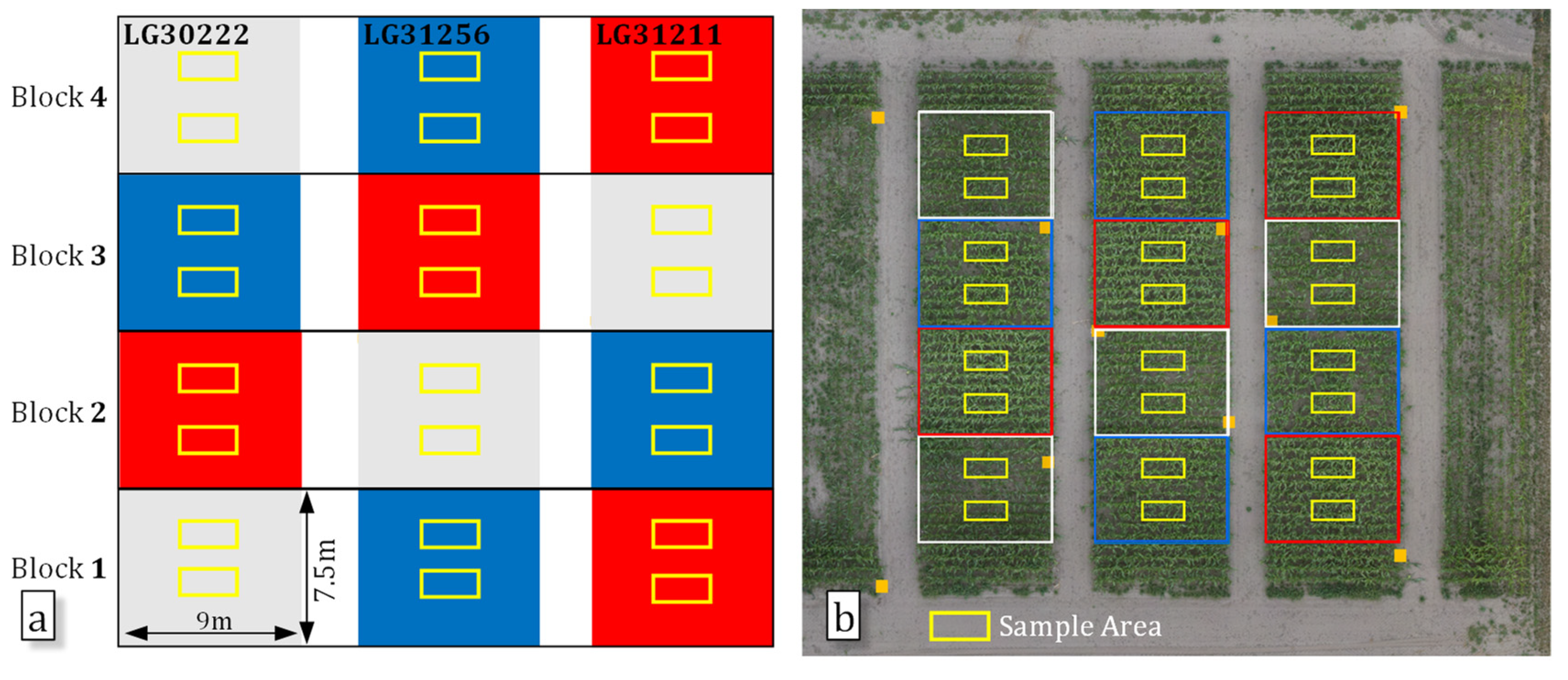
2.1. Field Preparation

All experiments and data collections were carried out between June and September of 2019, on a maize field at the Marquardt Digital Agriculture field of the Leibniz Institute for Agricultural Engineering and Bioeconomy, located in Potsdam, Germany (Lat: 52°28′01.2″N Lon: 12°57′20.9″E, Alt: 65–68 m). A map of the area is shown in Figure 3a. The landscape of the field was dominated by small-sized experimental plots containing other crops. The distribution of the maize field with 3 sub-plots is shown in Figure 3a. The study characterized three cultivars of maize with different canopy architectures that were cultivated in 12 plots over a total area of 48 by 36 m2. The maize field was seeded on 3 May 2019, with two rows per bed using a precision seeder (Terradonis company, La Jarrie, France) that was attached to a HEGE 76 farm-implement carrier (HEGE Maschinen, Hohebuch, Germany), as shown in Figure 3b. The seeder had two independent seeding units that were mounted on a bar and were then adjusted for a row spacing of 0.75 m spacing. The disk system was used to set a plant spacing of 0.25 m. The seed rate was equal through the experimental plots. Cultivation practices including irrigation, nutrition, fertilizer, and pesticide applications were performed by expert technicians. Figure 3c shows a view of the field at 26 days after sowing (DAS). Maize reached the growth stage of 13–15 on the Biologische Bundesanstalt, Bundessortenamt und CHemische Industrie (BBCH) scale code [74].

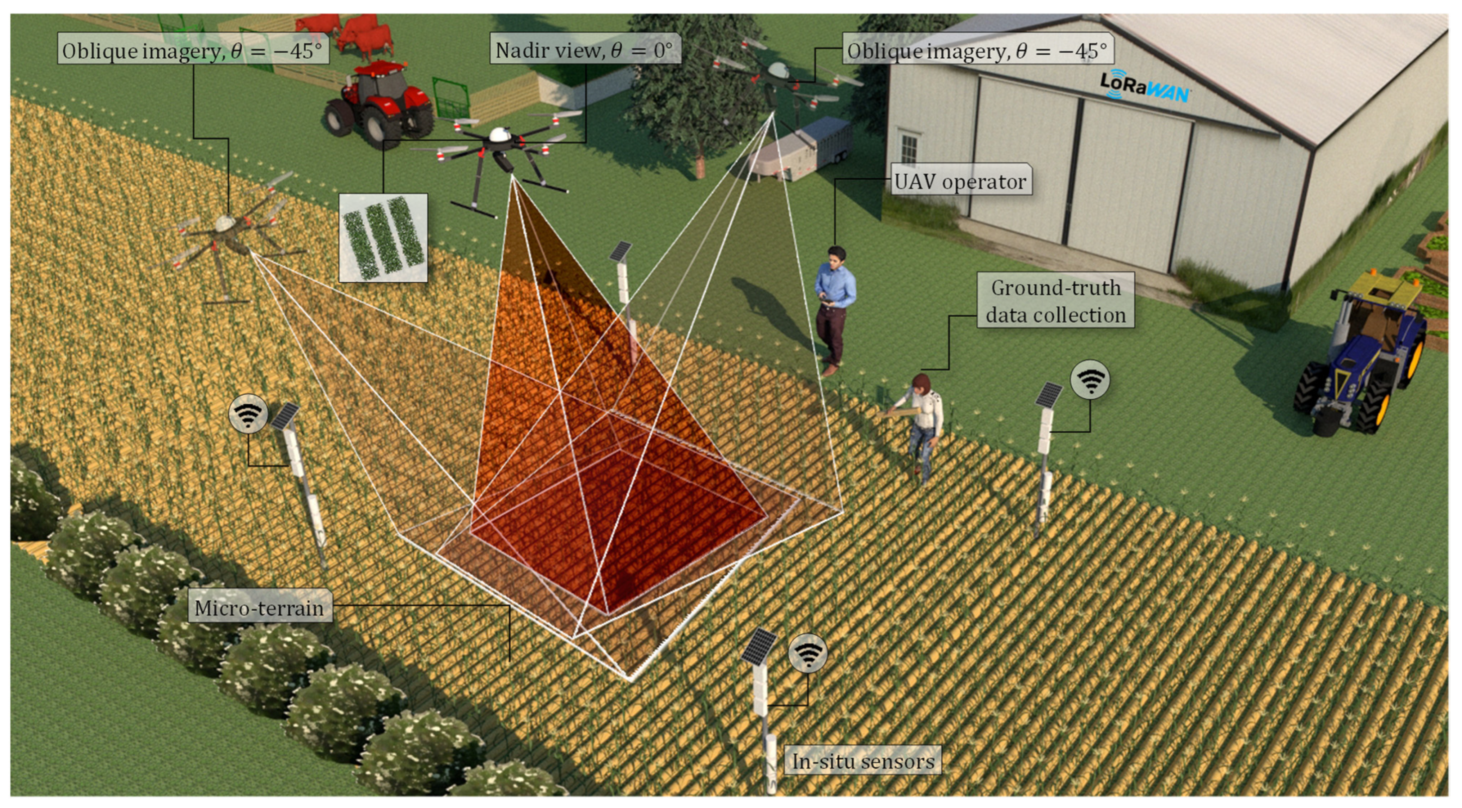
2.2. UAV-Image Acquisition and Manual Measurements

A multi-rotor unmanned aerial vehicle model HP-X4-E1200 (HEXAPILOTS, Dresden, Germany) equipped with a 2-axis gimbal, a Sony Alpha 6000 RGB camera (Sony Corporation, Tokyo, Japan), and a 16 mm lens were used to acquire RGB images in nadir and oblique view from the maize field at six different time slots during the growing season. The data collection setup and image acquisition hardware is shown in Figure 4. The camera was equipped with a 16 mm f/2.8 pancake lens, which provided a field-of-view equivalent to a classic 24 mm full format lens. The camera was mounted on the gimbal to provide nadir ( θ = 0 ° ) and oblique shooting angles ( θ = 45 ° ). During the image acquisition, the camera configuration mode was set to shutter 1/1000 s, ISO 100-200, F-stop auto, and daylight mode. An overlapping setting rate of 80% for both sides was employed to satisfy the Agisoft PhotoScan (Agisoft LLC, St. Petersburg, Russia) recommendation. The UAV and camera technical specifications used for this study of the crop estimation are listed in Table 2. The instruments used for ground-truth data collections were (i) SunScan LAI meter, (ii) ground control points (GCPs), and (iii) Topcon HiPer® Pro Differential Global Positioning System (DGPS).
The details of the six UAV flight campaigns are summarized in Table 3. Each flight task is labeled as A i N or A i O , where i is the index of the flight task, and N and O refers to the nadir and oblique views, respectively. The flight objective, growth stages, wind conditions, and the number of images collected during each flight are also given in Table 3. The first flight campaign (i.e., tasks A 1 N and A 1 O ) was performed as a pre-test for camera calibration, and to simulate the reference ground model with micro-terrain. The total of 2979 RGB images were collected in different wind speeds under clear sky conditions during eight back-and-forth flight lines with 5.87 m distance between the lines to cover the entire experimental plots in the maize field. The UAV was programmed to fly with ground speed of approximately 3 m/s at the heights that are given in Table 3. Images were collected continuously at an interval of 1 s, which resulted in a ground sampling distance (GSD) of approximately 5 mm/pixel. All images were taken from an equal distance to the surface of the canopy by applying different flight heights and flight route offset (FRO). The flight duration to complete image acquisition for each flight campaign was approximately between 25 and 35 min. It should be noted that the growth stage data given in Table 3 are based on the standard BBCH-scale code [74]. In addition, the wind speed data were provided by the Potsdam weather station located 11 km from the experimental site.

2.3. Ground-Truth Data Collection

Measurements of LAI and plants’ height were performed on the same day of the UAV flight campaigns. A screenshot of the map of the actual flight route and the flight control adjustments are shown in Figure 5. LAI was measured by a SunScan plant canopy analyzer system (SS1-COM-R4, Peak Design Ltd., Winster, UK). The analyzer system included a BF5 Sunshine Sensor, RadioLink components, a Personal Digital Assistant (PDA), a SunScan probe, and a tripod (shown earlier in Figure 4). The BF5 Sunshine Sensor was linked with the RadioLink component and then leveled by the three-axis tripod to record the above-canopy reference. The Handheld PDA is connected to the SunScan probe to collect and analyze readings from measurements. The system was used to measure the averaged LAI in sample areas for the canopy of different maize cultivars and growth variability. The plant height (PHT) and yield data were also collected according to agronomic reference measurements. Ground control points were designed to place in the field. They later were determined using the differential GPS HiPer Pro system (Topcon Corporation, Tokyo, Japan), having a relative horizontal and vertical accuracy of 3 and 5 mm (shown in Figure 5). It should be mentioned that the measurements did not involve any destructive sampling to record the lengths or the widths of the plants and leaves. In this study, the manually measured LAI and plant heights are referred to as actual measurements, while those extracted from UAV images are the estimated measurements.

2.4. Experimental Design and Statistical Analysis

Randomized complete block design (RCBD) was applied with the one-factor treatment and four replications, as shown in Figure 6. The factor is maize cultivar with three treatments (αi) for the contrasting canopy structures. Figure 6a,b show the schematic view of RCBD under study and the corresponding actual maize field layout. The field was split into four blocks (bj). Each block was divided into three experimental plots of equal size with ten rows. All three treatments were randomly assigned to the experimental plots in each block. The one-way analysis of variance (ANOVA) model can be stated as: yij =µ + αi + bj + ɛij. The maize cultivars are LG30222, LG31211, LG31256, respectively. Two cultivars, LG30222 and LG31211, have a reduced stature (not that high). Between the two of them, LG31211 has good development in the early growth stage and a leafier stature, and the third cultivar, LG31256, has a normal stature (higher canopy shape). Contrasting canopy structures were established in this way by three cultivars with their contrasting canopy architectures shown in Figure 6b. In addition, linear regression comparison analysis was performed to assess the performance of the UAV-SfM based method in estimating plant height and LAI across the maize field. The coefficients of determination (R2), root mean square error (RMSE), and relative root mean square error (rRMSE) described by the following equations were used to assess the degree of coincidence between ground truth and the estimated dataset. Here xi represents the field-observed value for sample area i , yi represents estimated value from image-based point clouds for sample area i , x ¯ and y ¯ are the average values, and n is the number of observed or estimated values in each dataset. The comparison was carried out for each growth stage separately and for all data pooled together.
R 2 = i = 1 n ( x i x ¯ ) 2 ( y i y ¯ ) 2 n i = 1 n ( x i x ¯ ) 2 i = 1 n ( y i y ¯ ) 2
RMSE = 1 n i = 1 n ( y i x i ) 2
rRMSE = RMSE x ¯ × 100 %

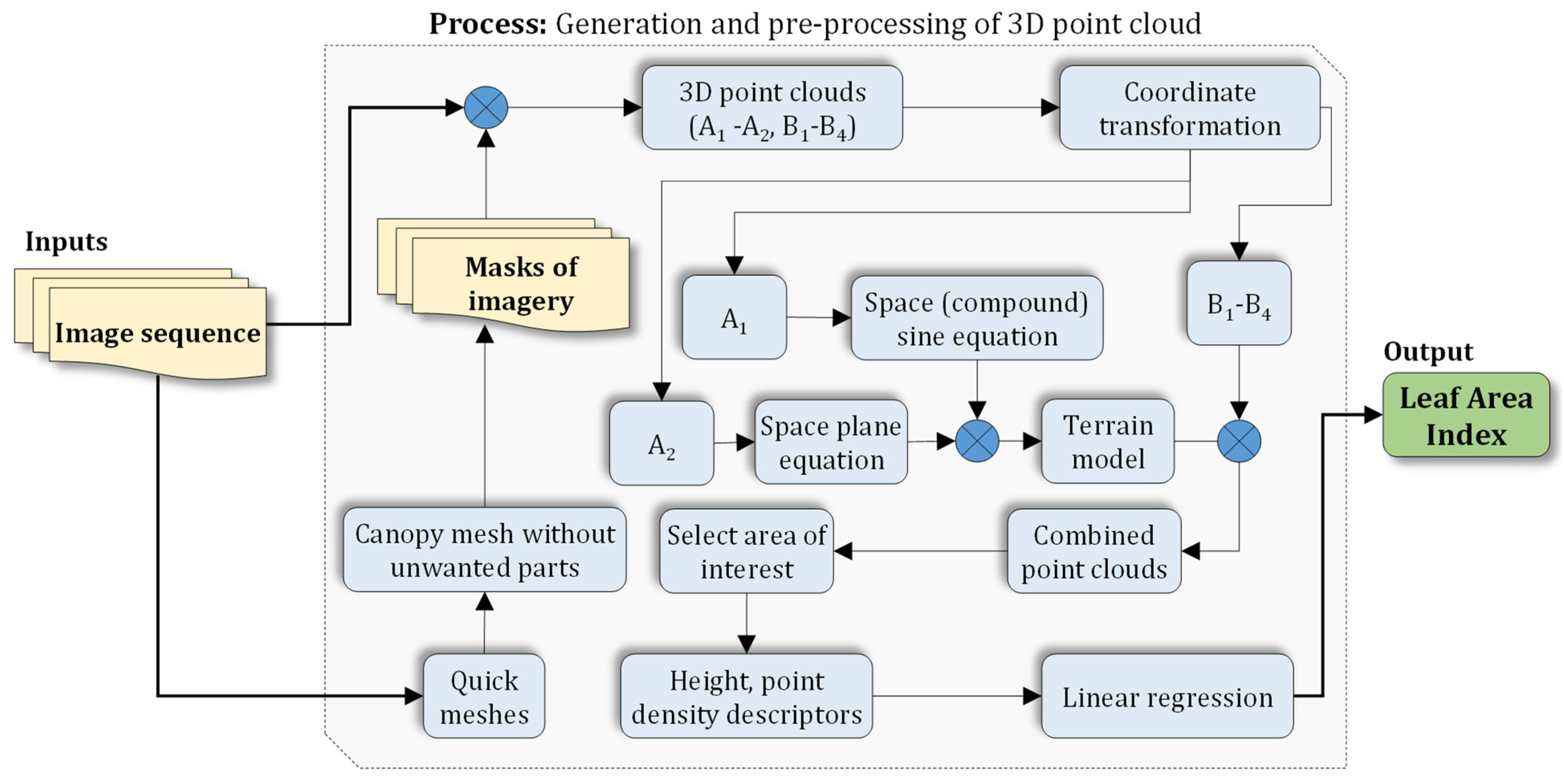
2.5. Generation and Pre-Processing of 3D Point Cloud

UAV images were processed using Agisoft Metashape Professional 1.7.3 (Agisoft LLC, St. Petersburg, Russia). The software uses SfM photogrammetry for generating 3D point clouds. For each growth stage, a 3D point cloud was generated from the nadir and oblique view set of images. The pre-processing steps included manual removal of invalid images (i.e., images that were acquired at the very beginning and end of the flight campaign, or those that were taken outside the field). The valid images from the six flight campaigns (A1–A2, B1–B4) were then imported to the Metashape, resulting in six individual image sequences which were processed individually by the software. For each image, maize canopy were separated from the soil and other undesired objects before modeling. This mask was created by the standard workflow for generating a quick mesh in Metashape. This step was required to improve the canopy model. Because most of the matching point pairs were extracted from irrelevant soil background, it reduced the usage of matching point pairs within the plant canopy. Prior to the image alignment, the mask was imported with the following software settings: method: from model, operation: replacement, and tolerance: 10. This approach avoided repetitive creation of masks for each individual image. The masks were then applied while generating the 3D point clouds using the SfM approach, including alignment, GCP labeling, gradual selection, and optimization procedure. Figure 7 illustrated the process of the generation of LAI from 3D point clouds using UAV RGB imagery. Here, the image sequences were used to create masks before 3D modeling and then the extracted masks of imagery were applied to generate the 3D point clouds (A1–A2, B1–B4). The point clouds were transformed to local coordinates. In the next step, the 3D point clouds A1–A2 were used for the derivation of the terrain model using a space (compound) sine equation and a space plane equation for the base-plane model, and the simulated micro-terrain. The terrain model was then merged with the 3D point clouds B1–B4 to obtain combined point clouds. The height, point density descriptors were calculated from the selected area of interest from the combined point clouds. The LAI were then calculated through a multivariate linear regression using height and point density descriptors in the select area of interest.
For quality optimization, 3D tie points were used from image alignment, which matched specific features in overlapping images. For these point clouds, a gradual selection procedure was used to identify and filter out low-quality points with the following user-defined criteria: reprojection error < 0.5 pixels, reconstruction uncertainty < 60, and projection error < 15. The filtered tie points were used to optimize the positions of the cameras using bundle adjustment. The resulting and optimized tie points were used as sparse point clouds. The sparse point clouds were georeferenced into the coordinate reference system ETRS89 UTM zone 33N (EPSG: 25833) and exported to PLY format. For further analysis in MATLAB, only the sparse point clouds were used as the 3D point clouds. This technique caused the point clouds to have the highest validity to the image feature matching [59]. Six individual point clouds, labeled as (A1–A2, B1–B4) were generated from the flight campaigns. In this scheme, a point cloud, i.e., A1, is defined as:
  P t C l o u d   A 1 = { [ φ i , λ i , ε i ] T R 3 ; i = 1 , , N A 1 }  
where φ i , λ i , and ε i are the value of eastings, northings, and altitude in meter of ith point of the P t C l o u d A 1 positioned in the UTM zone 33N, and N A 1 is the cardinality of the point cloud. The point clouds were split into k = 3 superplots Sk each covering an area of 9 by 36 m. To accelerate the next steps involving point clouds processing, a coordinate transformation was used to shift the superplots using Equation (5):
[ x y z ] = T [ φ x 1 λ y 1 ε ]  
where T = [ cos ( α )   sin ( α )   0 sin ( α )   cos ( α )   0 0   0   1 ] is the rotation matrix, and α is the rotation angle. The smallest value of φ and λ in the superplots was defined as ( x 1 , y 1 , 0 ) T , which is the translation vector to the origin ( 0 ,   0 ,   0 ) . After the rotations, the maize row of each S k is now parallel to the X-axis and vertical to Y-axis. P t C l o u d S k A s or P t C l o u d S k B s represent the superplots in local coordinates of each point cloud dataset and A1–A2 or B1–B4 are the identifiers of the point clouds. The example of a subset point cloud S 1 A 1 is defined as:
P t C l o u d S 1 A 1 = { [ x i , y i , z i ] T R 3 ; i = 1 , , N s 1 A 1 }
where x i , y i and z i are the value of X-axis, Y-axis, and altitude in meter of i t h point of the P t C l o u d S 1 A 1 in local coordinate transformation. N S 1 A 1 is the cardinality of the point cloud.

2.6. Derivation of Terrain Model

The terrain model was derived using a compound equation of two sine functions to simulate a curved surface that was constrained to point cloud P t c l o u d A 1 (early growth stage) with additional information of point cloud P t c l o u d A 2 (after tillage) for the base plane parameters. In the field, there is a periodic nature in the terrain present due to ridges and furrows that changes in the row direction. The difference of the peaks in a period is due to the rollers of field vehicles. To obtain the characteristics of this periodicity, soil points were extracted from P t c l o u d A 1 . The soil point section was then projected on the YZ-plane, and its characteristics were obtained through preliminary observations of the lower limit of the section, which has two-dimensionality and periodicity. These characteristics were used for defining the parameters A and B in Equation (7). Equation (7) describes the curve that characterizes this micro-terrain pattern by using a combined periodic piecewise sine function:
f ( t ) = { A × sin ( 2 π × rem ( t , T ) )   t ( r e m ( t , T ) 0.5 ,   0 t n   )   B × sin ( 2 π × ( rem ( t , T ) 0.5 ) )   t ( r e m ( t , T ) > 0.5 ,   0 t n ) ,
where A = 1 / 17 and B = 1 / 8 are the amplitudes, t is the position, T = 1.5   [ m ] is the period of the function representing two maize row spacing as one period, rem represents the remainder function, and n = 36 m is the total length of all rows. The axis of f ( t ) is defined as a tangent to the row direction and equal to the Y-axis. Then, based on the point cloud dataset P t c l o u d A 2 , the planar features of the superplots S 1 S 3 were extracted by estimating a plane from the point clouds using least squares approximation. The equation is expressed as:
z 0 k = a k x + b k y + c k   0 x m ,   0 y n
where a k , b k , c k are defined as values of the planar features, k is the index of the superplot (i.e., 1,2,3), x and y represent the point cloud positions, and m and n are the maximum size of the superplots in X and Y-axis, which are defined as 9 and 36 m. Finally, the parametrized plane curve f ( t ) (Equation (7)) was applied to the corresponding three planes z 0 k (Equation (8)). Consequently, the simulated terrain models were derived representing the micro-pattern features within plots S1S3, as follows:
Z k = { z k = a k x + b k y + c k + f ( y ) + c | 0 x m ,   0 y n   }
where c is a constant to adjust the height difference caused by tillage. Henceforth, only the simulated terrain model was used, and thus its explicit dependence on the ground surface point cloud was omitted. A schematic and two actual views of the ground surface are provided in Figure 8, showing ridges, row spacing and plant spacing of the ground surface (Figure 8a), and the nadir and side view of the actual field (Figure 8b,c).

2.7. Canopy Height Estimation

The following steps were used to estimate the canopy height from the point clouds. First, the middle part of the point clouds A S k ,   B s were extracted, which covered an area of 1 by 36 m along the middle line of superplot S k . It should be noted that the point clouds of the sample areas were included in the extraction. This resulted in three selections of points p i extracted from four point clouds with respect to the corresponding superplots ( S k ) and growth stages (s). The sample selection of the points in A S 1 ,   B 4 is given by Equation (10):
A S 1 ,   B 4 = { p i = [ x i , y i , z i ] T R 3 | | m 2 x i | 0.5 ,   0 y n , p i P t C l o u d S 1 ,   B 4 }
where point p i are the selection of the subset points. The selection of point clouds is thus constituted only by the points p i , representing maize canopy, from which the maize height will be extracted with respect to the terrain. The second step was to find the local peaks of the ridges from the simulated terrain model, which is a parametrized plane curve Z k . The peaks H k were detected by solving the local maximum problem:
H k = { q i = [ x , y , z ] T Z k | c = [ x c , y c , z c ] T Z k , c q , q i ( x , y ) z k ( x c , y c ) , }
where q i are the points on the ridges in the terrain model, point c Z k is the neighborhood of a point q i Z k , represented by coordinate values x c , y c , and z c . The third step was to obtain the height distribution of the canopy. For the sake of simplicity, 2D canopy maps A S k ,   B s 2 D were created with a dimensionality reduction of the subset 3D point clouds A S k ,   B s as given in Equation (12):
A S k ,   B s 2 D = { w i = [ x , y ] T R 2 | x = y , y = z , [ x , y , z ] T A S k ,   B s }   .
In order to avoid different slopes between the A S k ,   B s 2 D , the points were rotated slightly around the X-axis to match with the Y-axis. Figure 13d shows a sample of the resulting 2D canopy map A S 1 ,   B 4 2 D . Finally, the plant heights were calculated as the difference between the peak points of the ridges H k and the top percentiles of the point clouds (90% and 95%) in respect to the Z-axis. The two datasets were obtained from the field point clouds representing 24 sample areas including three cultivars. The canopy height-based values for sample areas were then used for estimating the crop height with a linear regression model. In this model, the dependent variable was the extracted height from the point cloud and the independent variable was the averaged plant height from field measurements.

2.8. Leaf Area Index Estimation

The following steps were used to estimate the LAI of the maize canopy from the point clouds A S k ,   B s 2 D . First, rectangular grids with different sizes were integrated into the point clouds A S k ,   B s 2 D to spatially divide the plant canopy and calculate the point density for each grid cell. Because the leaves and stems within the plant canopy are randomly distributed, the leaf area density of A S k ,   B s 2 D at the canopy level can be assumed as the point density of the grid. The density grids were used with sizes of 8, 15, and 25 cm. Equation (13) shows a matrix of the density grid distribution N S 1 ,   B 3 0.08 for the plant canopy with the grid size 8 cm (Figure 15a):
N S 1 ,   B 3 0.08 = { (   n u , v ) u × v   ,   w i A S 1 ,   B 3 2 D ,   u = x max x min 0.08 , v = y max y min 0.08   }
where   n u , v is the number of points measured in m 2 per grid, u and v are the number of grids in Y-axis and height directions, x max ,   x min ,   y max , and y min are the boundary values of the point cloud, 0.08 is the density grid size. The matrices with different grid sizes are represented as N S k ,   B s 0.08 , N S k ,   B s 0.15 , and N S k ,   B s 0.25 . The second step was to obtain a descriptor for the canopy density to describe the distribution for each sample area. For this purpose, a ratio was calculated between the amount of grid greater than w and the total map grid. The selected value of w was 0.2 × W S k ,   B s . Here, W S k ,   B s relates to the average point cloud density of the 2D canopy map obtained by dividing the total number of points by the area of the valid grids. Grid cells, where the density fall below the threshold w , were not used in the calculation of the descriptors. (Figure 14). Equation (14) refers to the descriptors for the sample areas in S 1 ,   B 3 :
D S 1 ,   B 3 = {   [ d 1 , r 0.08 ,   d 2 , r 0.15 ,   d 3 , r 0.25 ] 3 × 8 | d 1 , r 0.08 = f ( N S 1 ,   B 3 0.08 ) ,   d 2 , r 0.15 = f ( N S 1 ,   B 3 0.15 ) , d 3 , r 0.25 = f ( N S 1 ,   B 3 0.25 )   }
where function f ( N S 1 ,   B 3 0.08 ) , f ( N S 1 ,   B 3 0.15 ) and f ( N S 1 ,   B 3 0.25 )   were used to calculate the ratios for the sample areas. It varies between [0,1]. Finally, the LAI was calculated with respect to the several growth stages and cultivars. The relationship between the defined maize canopy descriptors and the LAI was described by a multivariate linear model as:
L A I = ( k = 1 2 c k . d k + q ) . δ 1
where k is the set of selected descriptors d k , which is the height and canopy density descriptor, c k is the coefficient of descriptor d k , q is the model intercept, and δ is the maize sample width, which is equal to 1 here. The LAI model was compared with field measurements to obtain the most reliable LAI descriptor.

3. Results and Discussion

3.1. Reconstructed 3D Point Clouds
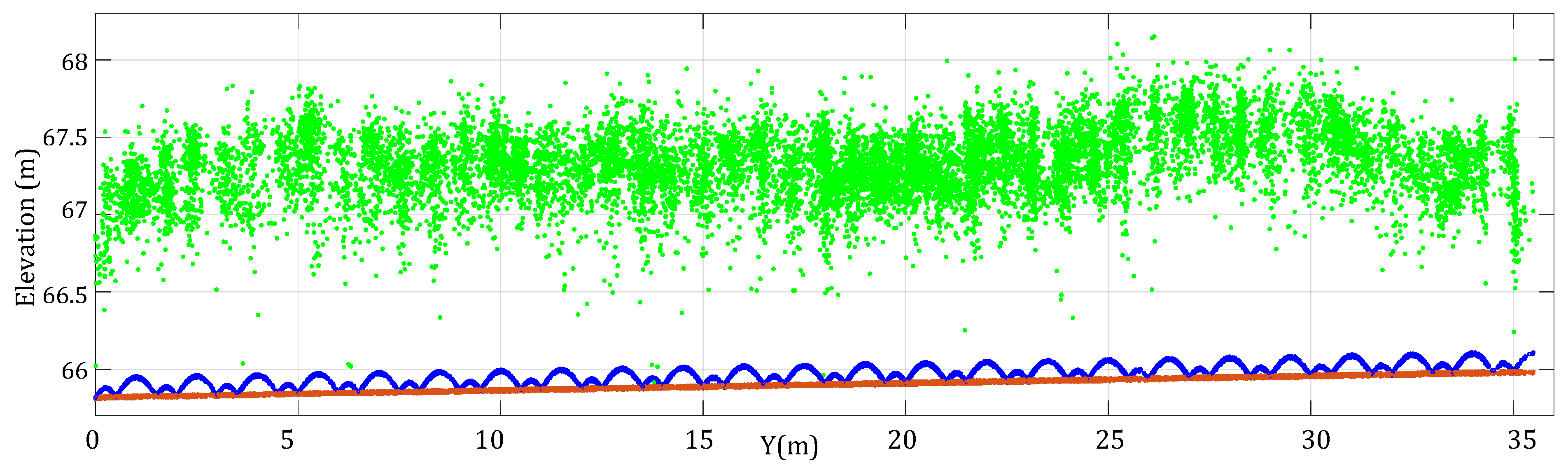
Reconstructed point clouds for the flight campaign of 31 July 2019, as well as camera locations and image overlap, ground control point locations, and digital elevation map, are shown in Figure 9. The 3D point cloud was processed by the SfM approach using image sequences that are masked shown in Figure 9a. It should be noted that ground pixels previously masked on the images were excluded from SfM procedures. A point cloud covering three superplots was created and used to extract the height and LAI values. Estimated camera locations are marked with a black dot, and numbers of the image overlap are indicated by coloring the position of recovery (Figure 9b). The image overlap reached 10 or more within the reconstructed canopy areas, indicating that every three images covered observed maize canopy effectively during the overflight. Figure 9c shows GCP locations and georeferencing precision on a spatial scale after filtering low-quality points. A total of 10 ellipses marked with dot points have been used to show the estimated GCP locations. These ellipses indicate the X (longitude), Y (latitude) errors of a reference point ranging between −1.9 and 4.6 cm. The estimated altitude accuracy (Z) is indicated by different colors representing the range between −0.79 and 0.63 cm. Figure 9d shows the reconstructed digital elevation. On this plot, the altitude ranges between 63.6 and 69.1 m, indicating the slope of the experimental site as well as the canopy height difference. The ground slope was considered in terrain model simulation after reconstruction.
The details of the result from the four flight campaigns, including the number of original images and aligned images after masking have been summarized in Table 4. These flight campaigns were performed as related to parameter estimation. Preliminary results showed that canopy pixels were prone to accurate reconstruction and georeferencing. The numbers of final images that were aligned after masking were between 561 and 616 for the four flight campaigns. The resulted ground sample distances (GSD) per campaign were between 5.64 and 5.84 mm. Reconstruction precision with original images and images after masking were found to be in the ranges of 1.5–2.0 mm and 1.7–2.0 mm, corresponding to average values of 1.7 and 1.85 mm, respectively. The increase from 1.7 to 1.85 is because of the exclusion of the soil ground pixels, which makes the image features more robust, which in the end, eliminates the error of matching pairs. Analysis of the data with t-test showed that the overall level of precision of point clouds resulted from original images, and aligned images were not significantly different. Georeferencing accuracy of the four campaigns resulted from the original images, and the aligned images were between 35.1 and 38.6 mm and 26.5–36.6 mm, respectively, showing a 21% (6.4 mm) improvement in the mean spatial accuracy.

3.2. Terrain Models

Sample graphical results corresponding to the derivation of the terrain model, including plots of the point cloud from the bare soil surface, the base-plane model, and the simulated terrain, are shown in Figure 10. The reconstructed soil point cloud generated from the tilled soil surface of superplot S 1 (as shown in Figure 10a), contains the general parameters of the ground surface. The plane parameters were obtained from the soil ground points within the corresponding area as a tilted space plane (Figure 10b). The simulated micro-terrain structure was applied to improve the general plane model by the piecewise Equation (7). It should be noted that the elevation of tilled soil decreases slightly than the previous seeded ground regarding the effect of tillage treatment. The terrain model was then generated from Equation (9), which included a factor to compensate for the difference between the tilled plane and the seeded ground. The result is shown by the simulated terrain of the field in Figure 10c.
Sample graphical results from the simulation of the micro-terrain structure are provided in Figure 11. It can be seen from the scatter plot of the terrain surface shown in Figure 11a that the discrete point data display a visible portion of point cloud A1 in view of the YZ-plane direction. While this sample of the reconstructed point cloud represented a relatively smooth and bare soil surface, the 3D point clouds still contained errors and noise, contributing to height differences that could reach 10 cm. This influenced the estimation of the height and LAI. For the sake of better investigation of the structure, Figure 11b shows the lower parts of the point cloud, which were more of interest by the simulation. By extracting the points, micro structure features revealed two sub-sections showing a curved profile. The extracted points were then used to fit the geometric characteristics using Equation (7) corresponding to the micro-terrain so as to make use of internal information in the point cloud. The simulated results of the micro-terrain structure were obtained and observed using the set of points in Figure 11c,d. The residual between the observed value and the simulated value is shown in Figure 11e. The results showed a high correlation between the model and points with residuals less than 3 to 4 cm. The micro-terrain in the ground surface corresponding to farm management can occur universally near the soil edges due to the effect of field machinery or vehicle developed across the field [75,76]. Lei et al. [1] obtained maize point cloud by LiDAR for LAI estimation, while ground point cloud was removed by de-noising and filtering. Christiansen et al. [50] studied the winter wheat crop and used only the pixel grid outside the plot to process a linear plane estimate for the soil surface. Information existing in point clouds can be repurposed to serve better and effective simulations and to support mining and use of internal information of point clouds (Figure 11). The residuals indicate the simulated structure can represent micro-terrain structure and proves effective at modeling the shape. Once the simulated ground surface was established using Equation (9) for superplots, a point cloud was built by combining the point simulated soil ground and the reconstructed maize canopy shown in Figure 12. As the ground surface was covered by maize canopy when the plant structure grew, these point clouds were used to the later canopy height estimation.

3.3. Height Estimation

The representative point clouds of maize canopies were derived from raw images and are demonstrated in Figure 13, showing the middle parts of the superplot S 1 over each growing season. The phenological stages of maize plants ranged from stem elongation with two nodes detectable (Figure 13a), to anthesis (Figure 13b), to end of flowering (Figure 13c), and to maturity (Figure 13d). It can be seen that the visualization of spatial arrangement for the maize canopy of point clouds varies depending on the dynamics of canopy growth. The differentiation of the canopy was structured according to plant coverage, leaf vitality, and degree of senescence. At the specific dates, the point clouds varied across the fields due to the difference in morphological performance between the three cultivars. Generally, thicker dense points indicate denser crop canopy, tighter structure, and higher plant vitality, whereas thinner sparser points are associated with sparser crop canopy. The differentiation gradually increased at the later dates.
The details of the models for estimation of the heights of the maize plant for each cultivar are given in Table 5. CH90 had a higher performance for the height estimation of all cultivars with different regression coefficients demonstrating that the three cultivars groups were statistically different in canopy shape. Except for the datasets corresponding to LG30256-CH95 (R2 = 0.46), General-CH95 (R2 = 0.60), and LG31211-CH95 (R2 = 0.67), other models showed a relatively high correlation between the actual (manual measurement) and estimated height. The reason for the low R2 of the mentioned cultivars is due to the reduced height of the structure of the samples. Plots of the correlation analysis between the actual and estimated height for each cultivar are provided in Figure 14. General models were provided by pooling all cultivars together and showed the model results and scatter plots. The plot labeled by LG30256-CH95 clearly shows the scattered points confirming the low R2. These plots also show the nature of the manual measurements that were carried out at four different growth stages, justifying the gap between the cultivars. Han et al. [28] studied canopy dynamics between different cultivars, and the results also supported the conclusion of this study that there were differences in the canopy dynamics results of crops at different growth stages. The bias between manually ruler measurement and point-derived plant height characterized by the RMSE also can come from that the average plant height was calculated to represent the height of the sample area.

3.4. LAI Estimation

A comparison between three kinds of scales for density divisions in the point cloud representing the maize crop superplot 1 acquired on 31 July 2019, is shown in Figure 15. These grids are the small scale of 0.08 × 0.08 m (Figure 15a), the medium scale of 0.15 × 0.15 m (Figure 15b), and the large scale of 0.25 × 0.25 m (Figure 15c), respectively. The color classification of the density was based on HSV color space. White/blank area indicated none of the points generated in this area, whereas varying color space indicated the varying density and condition of the maize canopy. Density distribution maps allowed observation of plant canopy and differentiation of canopy structure of varying density. The maize formed a continuous canopy of varying density from the image-based point clouds. The common characteristic was red profiles of grids scattered around the green core areas of varying density. The canopy structure description from point clouds was most similar to the map from the small-scale density grid. Additionally, the crop canopy rows, and their gaps were well-distinguished, which can also be seen in the plots from the early to maturity growth stages in Figure 15. However, two types of differences were found between the density maps divided under the three tested grids cells. First, based on the range of canopy densities, it was recognized that individual canopy density maps could have extremely high point cloud density values locally, especially in the core of the canopy in the small-scale grid division. The strong density can be explained by leaves, branches, and other parts being significantly concentrated in these areas and therefore forming a more robust occlusion. Second, along the maize rows, the density map showed a variation in density, whereas the variation tends to be weaker in density maps of larger-scale gridding. The loss of detail in larger grids can also be anticipated from the row spacing, which is 0.75 m. Moreover, in the small-scale canopy density map, it is possible to observe more contours and gaps because of the good discrimination along crop rows and gaps and also to identify the differences between varieties.
A more detailed comparison of point density maps for maize (18 m long) canopy of S 1 over different growth stages is shown in Figure 16. As shown before, from the point density maps and based on the UAV point clouds, it was possible to accurately map the general structures, such as corn crop contours and gaps. Due to the heterogeneous point distribution by the SfM method, it can be noticed that the point density showed variability within structures even rendered core canopy structure of maize. In this set of examples, the first density map (Figure 16a) showed canopy structures that were visually about the internal and row gaps, as can be seen in the early growth stage. Subsequently, the gap was gradually filled by both sides of the crop, and the core structures of the canopy gradually expanded (Figure 16b,c). In the last growth stage shown in the plot of Figure 16d, the gaps increased once more, whereas overall showed a more porous profile. In this scenario, the mature canopy was estimated to be relatively small and therefore was the sparsest. When comparing the height and LAI, the height difference between the third and fourth growth stages was relatively small, but the difference in the measured LAI estimates had a downward trend to some extent. In general, the point density values were compared and estimated laterally within point clouds of the same growth stage for canopy structure. When comparing two and more growth stages, point density values were, to some extent, influenced by wind speed, ambient light, reconstruction effect, and other field disturbances. Therefore, the average density values were used to unify the different point cloud images.
An example of the set of descriptors and calculated values for sample area 1 is given in Table 6. In particular, a set of five descriptors was calculated for all sample areas, two of which, CH 95 and CH 90 , are related to the height of the canopy, and three of which, D 0.08 , D 0.15 , and D 0.25 are related to the density distribution of the sample areas. In the considered sample areas, the canopy thickness is the width of the subset of the maize point cloud in the X-axis, and the thickness is consistent among sample areas. Figure 17 shows the measured and estimated LAI at four growth stages in an order of index of the sample area. LAI values compared with traditional manual method. The reference manual measured LAI (Figure 17a) was shown by scatter points and line graphs among the different growth stages. Estimated LAI values were plotted in the relation to the manual-measured LAI in Figure 17b. The LAI estimation of maize from sparse point cloud by the proposed methodology was able to estimate the LAI from the dataset of descriptors. Based on the multivariate linear regression model, CH90 was tested as the most effective descriptors of height for all cultivars. D 0.08 concluded as the best density descriptor among cultivar LG30222 and LG31256 and D 0.25 was the best density descriptor for LG31211. LAI for these three cultivars are also different. Large-scale canopy density descriptors are suitable for more sparer and/or higher canopy structures, while small-scale canopy density descriptors are more effective with the leafy and reduced canopy structure which were extracted from the 3D point clouds. The best correlation is R2 = 0.48 because of the missing of some maize plants, which makes the reduced density of canopy for seven sample areas in four plots, which at the end decreased the estimated LAI. Figure 18 shows actual and estimated averaged LAI in each field plot and the corresponding estimated error (%). Figure 18a shows some good agreement between the estimated averaged and averaged measured LAI at plot-level over the 12 plots for all growth stages. The estimated averaged LAI was relatively similar to the actual averaged LAI in the plots with well-germinated seeds that were not affected by lodging. In the plots where the corresponding sample areas contained poorly germinated seeds or lodged plants, the canopy tended to be at least partly reduced [77], whereas the separation for the partial point cloud regions of non-plant objects was still difficult. Plant density descriptors in these sample areas can be smaller compared to those sample areas that recorded non-missing plants. As a result, in the field plots 3, 6, 9, and 12, it is possible to observe more significant estimated errors and lower estimated LAI values due to the missing of some maize plants within the area (Figure 18a,b). Point cloud density inside the canopy was a major factor causing the underestimation of the LAI because the effect of the missing plants was underestimated. The result in Figure 18 showed information about the crop regarding height, in particularly, canopy density, canopy width, or inter-row space are of interest for the nondestructive assessments of the vegetation biophysical parameters [23]. As an application of spatial point cloud density-related parameter estimation, how to filter out the partial point cloud regions of non-plant objects needs to be further considered in the calculation of spatial density descriptors (D0.08, D0.15, D0.25) of different grid sizes.

4. Conclusions

LAI and height of maize were estimated in this study using canopy height and point density descriptors processed through acquired UAV 3D data to investigate a cost-effective and high-resolution alternative to the conventional in-field measurement. The study used an unmanned aerial system to acquire nadir and oblique images of maize canopy from approximately 20 m distance from the canopy surface for reconstructing 3D point clouds using the SfM approach. The following conclusions can be drawn for the indirect 3D imaging approach of the maize height and LAI.
  • Before the estimation, the reference ground model with micro-terrain was derived and then simulated with a curved surface to be used to identify the canopy features. Including the micro-terrain in the ground, the model was found suitable for extracting the parameters of maize during the growing season in more detail.
  • Except for the datasets corresponding to LG30256-CH95 (R2 = 0.46) and LG31211-CH95 (R2 = 0.67), the height estimation of maize achieved a relatively high correlation (R2 = 0.89, 0.86, 0.78) for cultivar datasets LG30222-CH90, LG31256-CH90, and LG31211-CH90 between the estimated and actual data, indicating effective modeling by point cloud data. Additionally, a general model for height estimation was derived for all three cultivar datasets with an R2 of 0.80 in CH90. This could be beneficial to breeding experiments.
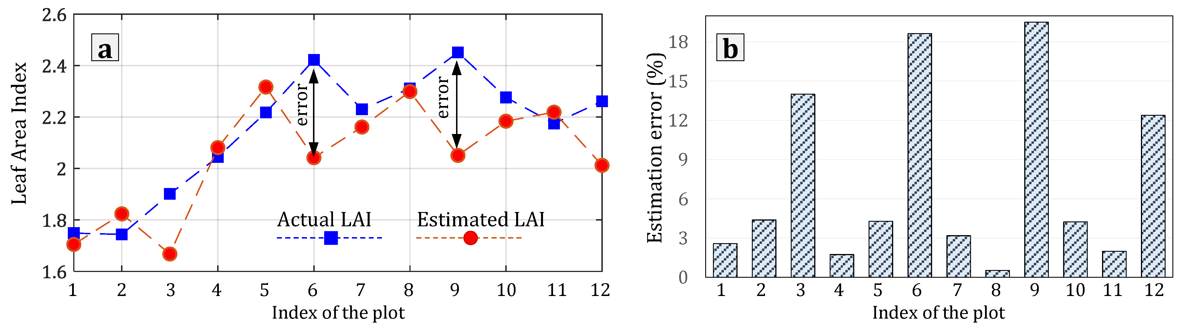
  • The correlation of LAI estimation was less desirable (R2 = 0.48) due to lower point density values caused by the missing maize plants in the sample areas (i.e., lodging, failure of seed germination), leading to a different and uneven number of maize in the areas and thus inaccurate estimation of canopy density and LAI. This should also be investigated further.
It is necessary to address the aforementioned issues and provide improved approaches in both field data collection and data processing for labeling and filtering out the regions of non-plant objects resulting in the error of spatial point cloud density-related parameters, such as canopy density and LAI. Future studies will also focus on the development of the approached methods with descriptors for further genotype differentiation in maize plants within a largescale field. The approach of mapping the canopy height and LAI in a field condition through the UAV platform would be particularly useful for supporting precision agriculture and digital farming applications, such as fertilization, breeding project, and yield prediction due to the versatility, flexibility, and low operational costs. The proposed methodology allows automatic measurement of LAI with high resolution and fast intensive mapping of in-field LAI index extraction from UAV 3D data of a field. Spatial and temporal data with high resolution is therefore assessable at an affordable cost with respect to conventional manual measurements.

Author Contributions

Conceptualization, M.L., M.S.L., R.R.S. and M.S.; methodology, M.L., M.S.L., R.R.S. and M.S.; software, M.L., M.S., R.R.S. and S.S.; validation, M.L., M.S., R.R.S. and S.S.; formal analysis, M.L., R.R.S. and M.S.; investigation, M.L. and R.R.S.; resources, C.W.; data curation, M.L. and R.R.S.; writing—original draft preparation, M.L. and R.R.S.; writing—review and editing, R.R.S., M.L., M.S. and S.S.; visualization, M.L. and R.R.S.; supervision, M.S.L., R.R.S., M.S., C.W. and S.S; project administration, C.W.; funding acquisition, C.W. and M.L. All authors have read and agreed to the published version of the manuscript.

Funding

This research received no external funding.

Institutional Review Board Statement

Not applicable.

Informed Consent Statement

Not applicable.

Data Availability Statement

Data are contained within the article.

Acknowledgments

The authors would like to acknowledge the support from the China Scholarship Council (CSC), the Leibniz Institute for Agricultural Engineering and Bioeconomy (ATB), and Technische Universität Berlin (TU Berlin). The fieldwork and data collection support from Antje Giebel and Marc Zimne are duly acknowledged. The publication has been funded by the Leibniz Open Access Publishing Fund.

Conflicts of Interest

The authors declare no conflict of interest.

References

  1. Lei, L.; Qiu, C.; Li, Z.; Han, D.; Han, L.; Zhu, Y.; Wu, J.; Xu, B.; Feng, H.; Yang, H. Effect of leaf occlusion on leaf area index inversion of maize using UAV–LiDAR data. Remote Sens. 2019, 11, 1067. [Google Scholar] [CrossRef] [Green Version]
  2. Rodrigo-Comino, J. Five decades of soil erosion research in “terroir”. The State-of-the-Art. Earth-Sci. Rev. 2018, 179, 436–447. [Google Scholar] [CrossRef]
  3. Chen, S.; Wang, J.; Zhang, T.; Hu, Z.; Zhou, G. Warming and straw application increased soil respiration during the different growing seasons by changing crop biomass and leaf area index in a winter wheat-soybean rotation cropland. Geoderma 2021, 391, 114985. [Google Scholar] [CrossRef]
  4. Anwar, S.A. On the contribution of dynamic leaf area index in simulating the African climate using a regional climate model (RegCM4). Theor. Appl. Climatol. 2021, 143, 119–129. [Google Scholar] [CrossRef]
  5. Mourad, R.; Jaafar, H.; Anderson, M.; Gao, F. Assessment of Leaf Area Index Models Using Harmonized Landsat and Sentinel-2 Surface Reflectance Data over a Semi-Arid Irrigated Landscape. Remote Sens. 2020, 12, 3121. [Google Scholar] [CrossRef]
  6. Paul, M.; Rajib, A.; Negahban-Azar, M.; Shirmohammadi, A.; Srivastava, P. Improved agricultural Water management in data-scarce semi-arid watersheds: Value of integrating remotely sensed leaf area index in hydrological modeling. Sci. Total Environ. 2021, 791, 148177. [Google Scholar] [CrossRef]
  7. Zhou, L.; Gu, X.; Cheng, S.; Yang, G.; Shu, M.; Sun, Q. Analysis of plant height changes of lodged maize using UAV-LiDAR data. Agriculture 2020, 10, 146. [Google Scholar] [CrossRef]
  8. Herrmann, I.; Bdolach, E.; Montekyo, Y.; Rachmilevitch, S.; Townsend, P.A.; Karnieli, A. Assessment of maize yield and phenology by drone-mounted superspectral camera. Precis. Agric. 2020, 21, 51–76. [Google Scholar] [CrossRef]
  9. Nguy-Robertson, A.L.; Peng, Y.; Gitelson, A.A.; Arkebauer, T.J.; Pimstein, A.; Herrmann, I.; Karnieli, A.; Rundquist, D.C.; Bonfil, D.J. Estimating green LAI in four crops: Potential of determining optimal spectral bands for a universal algorithm. Agric. For. Meteorol. 2014, 192, 140–148. [Google Scholar] [CrossRef]
  10. Monsi, M. Uber den Lichtfaktor in den Pflanzen-gesellschaften und seine Bedeutung fur die Stoffproduktion [On the light factor in plant societies and ist significance for substance production]. Jap. Journ. Bot. 1953, 14, 22–52. [Google Scholar]
  11. Yan, G.; Hu, R.; Luo, J.; Weiss, M.; Jiang, H.; Mu, X.; Xie, D.; Zhang, W. Review of indirect optical measurements of leaf area index: Recent advances, challenges, and perspectives. Agric. For. Meteorol. 2019, 265, 390–411. [Google Scholar] [CrossRef]
  12. Kerkech, M.; Hafiane, A.; Canals, R. Deep leaning approach with colorimetric spaces and vegetation indices for vine diseases detection in UAV images. Comput. Electron. Agric. 2018, 155, 237–243. [Google Scholar] [CrossRef]
  13. Deery, D.M.; Rebetzke, G.J.; Jimenez-Berni, J.A.; Condon, A.G.; Smith, D.J.; Bechaz, K.M.; Bovill, W.D. Ground-based LiDAR improves phenotypic repeatability of above-ground biomass and crop growth rate in wheat. Plant Phenomics 2020, 2020, 8329798. [Google Scholar] [CrossRef] [PubMed]
  14. Jiang, Y.; Li, C.; Takeda, F.; Kramer, E.A.; Ashrafi, H.; Hunter, J. 3D point cloud data to quantitatively characterize size and shape of shrub crops. Hortic. Res. 2019, 6, 43. [Google Scholar] [CrossRef] [Green Version]
  15. Zhang, X.; Ren, Y.; Yin, Z.Y.; Lin, Z.; Zheng, D. Spatial and temporal variation patterns of reference evapotranspiration across the Qinghai-Tibetan Plateau during 1971–2004. J. Geophys. Res. Atmos. 2009, 114. [Google Scholar] [CrossRef]
  16. Hardin, P.J.; Jensen, R.R. Small-Scale Unmanned Aerial Vehicles in Environmental Remote Sensing: Challenges and Opportunities. GIScience Remote Sens. 2011, 48, 99–111. [Google Scholar] [CrossRef]
  17. Knoth, C.; Klein, B.; Prinz, T.; Kleinebecker, T. Unmanned aerial vehicles as innovative remote sensing platforms for high-resolution infrared imagery to support restoration monitoring in cut-over bogs. Appl. Veg. Sci. 2013, 16, 509–517. [Google Scholar] [CrossRef]
  18. Linchant, J.; Lisein, J.; Semeki, J.; Lejeune, P.; Vermeulen, C. Are unmanned aircraft systems (UASs) the future of wildlife monitoring? A review of accomplishments and challenges. Mamm. Rev. 2015, 45, 239–252. [Google Scholar] [CrossRef]
  19. Whitehead, K.; Hugenholtz, C.H.; Myshak, S.; Brown, O.; LeClair, A.; Tamminga, A.; Barchyn, T.E.; Moorman, B.; Eaton, B. Remote sensing of the environment with small unmanned aircraft systems (UASs), part 2: Scientific and commercial applications. J. Unmanned Veh. Syst. 2014, 2, 86–102. [Google Scholar] [CrossRef] [Green Version]
  20. Shahbazi, M.; Théau, J.; Ménard, P. Recent applications of unmanned aerial imagery in natural resource management. GIScience Remote Sens. 2014, 51, 339–365. [Google Scholar] [CrossRef]
  21. Wallace, L.; Lucieer, A.; Watson, C.; Turner, D. Development of a UAV-LiDAR System with Application to Forest Inventory. Remote Sens. 2012, 4, 1519–1543. [Google Scholar] [CrossRef] [Green Version]
  22. Shamshiri, R.R. Fundamental Research on Unmanned Aerial Vehicles to Support Precision Agriculture in Oil Palm Plantations; Hameed, I.A., Ed.; IntechOpen: Rijeka, Croatia, 2019; Chapter 6; pp. 91–116. ISBN 978-1-78984-934-9. [Google Scholar]
  23. Comba, L.; Biglia, A.; Ricauda Aimonino, D.; Tortia, C.; Mania, E.; Guidoni, S.; Gay, P. Leaf Area Index evaluation in vineyards using 3D point clouds from UAV imagery. Precis. Agric. 2020, 21, 881–896. [Google Scholar] [CrossRef] [Green Version]
  24. Garcerá, C.; Doruchowski, G.; Chueca, P. Harmonization of plant protection products dose expression and dose adjustment for high growing 3D crops: A review. Crop Prot. 2021, 140, 105417. [Google Scholar] [CrossRef]
  25. Bates, J.S.; Montzka, C.; Schmidt, M.; Jonard, F. Estimating Canopy Density Parameters Time-Series for Winter Wheat Using UAS Mounted LiDAR. Remote Sens. 2021, 13, 710. [Google Scholar] [CrossRef]
  26. Vergara-Díaz, O.; Zaman-Allah, M.A.; Masuka, B.; Hornero, A.; Zarco-Tejada, P.; Prasanna, B.M.; Cairns, J.E.; Araus, J.L. A Novel Remote Sensing Approach for Prediction of Maize Yield Under Different Conditions of Nitrogen Fertilization. Front. Plant Sci. 2016, 7, 666. [Google Scholar] [CrossRef] [Green Version]
  27. Guo, W.; Carroll, M.E.; Singh, A.; Swetnam, T.L.; Merchant, N.; Sarkar, S.; Singh, A.K.; Ganapathysubramanian, B. UAS-Based Plant Phenotyping for Research and Breeding Applications. Plant Phenomics 2021, 2021, 9840192. [Google Scholar] [CrossRef]
  28. Han, L.; Yang, G.; Yang, H.; Xu, B.; Li, Z.; Yang, X. Clustering field-based maize phenotyping of plant-height growth and canopy spectral dynamics using a UAV remote-sensing approach. Front. Plant Sci. 2018, 9, 1638. [Google Scholar] [CrossRef] [Green Version]
  29. Herrero-Huerta, M.; González-Aguilera, D.; Rodriguez-Gonzalvez, P.; Hernández-López, D. Vineyard yield estimation by automatic 3D bunch modelling in field conditions. Comput. Electron. Agric. 2015, 110, 17–26. [Google Scholar] [CrossRef]
  30. Torres-Sánchez, J.; de Castro, A.I.; Peña, J.M.; Jiménez-Brenes, F.M.; Arquero, O.; Lovera, M.; López-Granados, F. Mapping the 3D structure of almond trees using UAV acquired photogrammetric point clouds and object-based image analysis. Biosyst. Eng. 2018, 176, 172–184. [Google Scholar] [CrossRef]
  31. Jiménez-Brenes, F.M.; López-Granados, F.; de Castro, A.I.; Torres-Sánchez, J.; Serrano, N.; Peña, J.M. Quantifying pruning impacts on olive tree architecture and annual canopy growth by using UAV-based 3D modelling. Plant Methods 2017, 13, 55. [Google Scholar] [CrossRef] [Green Version]
  32. Mathews, A.; Jensen, J. Visualizing and Quantifying Vineyard Canopy LAI Using an Unmanned Aerial Vehicle (UAV) Collected High Density Structure from Motion Point Cloud. Remote Sens. 2013, 5, 2164–2183. [Google Scholar] [CrossRef] [Green Version]
  33. Hobart, M.; Pflanz, M.; Weltzien, C.; Schirrmann, M. Growth Height Determination of Tree Walls for Precise Monitoring in Apple Fruit Production Using UAV Photogrammetry. Remote Sens. 2020, 12, 1656. [Google Scholar] [CrossRef]
  34. Guo, Y.; Chen, S.; Wu, Z.; Wang, S.; Robin Bryant, C.; Senthilnath, J.; Cunha, M.; Fu, Y.H. Integrating Spectral and Textural Information for Monitoring the Growth of Pear Trees Using Optical Images from the UAV Platform. Remote Sens. 2021, 13, 1795. [Google Scholar] [CrossRef]
  35. Che, Y.; Wang, Q.; Xie, Z.; Zhou, L.; Li, S.; Hui, F.; Wang, X.; Li, B.; Ma, Y. Estimation of maize plant height and leaf area index dynamics using an unmanned aerial vehicle with oblique and nadir photography. Ann. Bot. 2020, 126, 765–773. [Google Scholar] [CrossRef]
  36. Li, B.; Xu, X.; Zhang, L.; Han, J.; Bian, C.; Li, G.; Liu, J.; Jin, L. Above-ground biomass estimation and yield prediction in potato by using UAV-based RGB and hyperspectral imaging. ISPRS J. Photogramm. Remote Sens. 2020, 162, 161–172. [Google Scholar] [CrossRef]
  37. Cucchiaro, S.; Fallu, D.J.; Zhang, H.; Walsh, K.; Van Oost, K.; Brown, A.G.; Tarolli, P. Multiplatform-SfM and TLS data fusion for monitoring agricultural terraces in complex topographic and landcover conditions. Remote Sens. 2020, 12, 1946. [Google Scholar] [CrossRef]
  38. Nesbit, P.R.; Hugenholtz, C.H. Enhancing UAV-SfM 3D model accuracy in high-relief landscapes by incorporating oblique images. Remote Sens. 2019, 11, 239. [Google Scholar] [CrossRef] [Green Version]
  39. Volpato, L.; Pinto, F.; González-Pérez, L.; Thompson, I.G.; Borém, A.; Reynolds, M.; Gérard, B.; Molero, G.; Rodrigues, F.A., Jr. High throughput field phenotyping for plant height using UAV-based RGB imagery in wheat breeding lines: Feasibility and validation. Front. Plant Sci. 2021, 12, 185. [Google Scholar] [CrossRef]
  40. Duan, B.; Liu, Y.; Gong, Y.; Peng, Y.; Wu, X.; Zhu, R.; Fang, S. Remote estimation of rice LAI based on Fourier spectrum texture from UAV image. Plant Methods 2019, 15, 124. [Google Scholar] [CrossRef] [Green Version]
  41. Lin, C.-W.; Ding, Q.; Tu, W.-H.; Huang, J.-H.; Liu, J.-F. Fourier dense network to conduct plant classification using UAV-based optical images. IEEE Access 2019, 7, 17736–17749. [Google Scholar] [CrossRef]
  42. Zheng, Q.; Huang, W.; Ye, H.; Dong, Y.; Shi, Y.; Chen, S. Using continous wavelet analysis for monitoring wheat yellow rust in different infestation stages based on unmanned aerial vehicle hyperspectral images. Appl. Opt. 2020, 59, 8003–8013. [Google Scholar] [CrossRef] [PubMed]
  43. Hasan, M.M.; Chopin, J.P.; Laga, H.; Miklavcic, S.J. Detection and analysis of wheat spikes using Convolutional Neural Networks. Plant Methods 2018, 14, 100. [Google Scholar] [CrossRef] [PubMed] [Green Version]
  44. Yamaguchi, T.; Tanaka, Y.; Imachi, Y.; Yamashita, M.; Katsura, K. Feasibility of Combining Deep Learning and RGB Images Obtained by Unmanned Aerial Vehicle for Leaf Area Index Estimation in Rice. Remote Sens. 2021, 13, 84. [Google Scholar] [CrossRef]
  45. Li, Y.; Wen, W.; Guo, X.; Yu, Z.; Gu, S.; Yan, H.; Zhao, C. High-throughput phenotyping analysis of maize at the seedling stage using end-to-end segmentation network. PLoS ONE 2021, 16, e0241528. [Google Scholar] [CrossRef] [PubMed]
  46. Dhakal, M.; Locke, M.A.; Huang, Y.; Reddy, K.; Moore, M.T.; Krutz, J. Estimation of Cotton and Sorghum Crop Density and Cover at Early Vegetative Stages Using Unmanned Aerial Vehicle Imagery. In Proceedings of the AGU Fall Meeting Abstracts, online, 1–17 December 2020; Volume 2020, p. GC023-0005. [Google Scholar]
  47. Maimaitiyiming, M.; Sagan, V.; Sidike, P.; Kwasniewski, M.T. Dual activation function-based Extreme Learning Machine (ELM) for estimating grapevine berry yield and quality. Remote Sens. 2019, 11, 740. [Google Scholar] [CrossRef] [Green Version]
  48. Madec, S.; Baret, F.; De Solan, B.; Thomas, S.; Dutartre, D.; Jezequel, S.; Hemmerlé, M.; Colombeau, G.; Comar, A. High-throughput phenotyping of plant height: Comparing unmanned aerial vehicles and ground LiDAR estimates. Front. Plant Sci. 2017, 8, 2002. [Google Scholar] [CrossRef] [Green Version]
  49. ten Harkel, J.; Bartholomeus, H.; Kooistra, L. Biomass and crop height estimation of different crops using UAV-based LiDAR. Remote Sens. 2020, 12, 17. [Google Scholar] [CrossRef] [Green Version]
  50. Christiansen, M.P.; Laursen, M.S.; Jørgensen, R.N.; Skovsen, S.; Gislum, R. Designing and Testing a UAV Mapping System for Agricultural Field Surveying. Sensors 2017, 17, 2703. [Google Scholar] [CrossRef] [Green Version]
  51. Jay, S.; Rabatel, G.; Hadoux, X.; Moura, D.; Gorretta, N. In-field crop row phenotyping from 3D modeling performed using Structure from Motion. Comput. Electron. Agric. 2015, 110, 70–77. [Google Scholar] [CrossRef] [Green Version]
  52. Tian, J.; Wang, L.; Li, X.; Gong, H.; Shi, C.; Zhong, R.; Liu, X. Comparison of UAV and WorldView-2 imagery for mapping leaf area index of mangrove forest. Int. J. Appl. Earth Obs. Geoinf. 2017, 61, 22–31. [Google Scholar] [CrossRef]
  53. Córcoles, J.I.; Ortega, J.F.; Hernández, D.; Moreno, M.A. Estimation of leaf area index in onion (Allium cepa L.) using an unmanned aerial vehicle. Biosyst. Eng. 2013, 115, 31–42. [Google Scholar] [CrossRef]
  54. Lendzioch, T.; Langhammer, J.; Jenicek, M. Estimating snow depth and leaf area index based on UAV digital photogrammetry. Sensors 2019, 19, 1027. [Google Scholar] [CrossRef] [PubMed] [Green Version]
  55. Sha, Z.; Wang, Y.; Bai, Y.; Zhao, Y.; Jin, H.; Na, Y.; Meng, X. Comparison of leaf area index inversion for grassland vegetation through remotely sensed spectra by unmanned aerial vehicle and field-based spectroradiometer. J. Plant Ecol. 2018, 12, 395–408. [Google Scholar] [CrossRef] [Green Version]
  56. Roosjen, P.P.J.; Brede, B.; Suomalainen, J.M.; Bartholomeus, H.M.; Kooistra, L.; Clevers, J.G.P.W. Improved estimation of leaf area index and leaf chlorophyll content of a potato crop using multi-angle spectral data—Potential of unmanned aerial vehicle imagery. Int. J. Appl. Earth Obs. Geoinf. 2018, 66, 14–26. [Google Scholar] [CrossRef]
  57. Lin, Y.; Jiang, M.; Yao, Y.; Zhang, L.; Lin, J. Use of UAV oblique imaging for the detection of individual trees in residential environments. Urban For. Urban Green. 2015, 14, 404–412. [Google Scholar] [CrossRef]
  58. Atkins, J.W.; Stovall, A.E.L.; Yang, X. Mapping temperate forest phenology using tower, UAV, and ground-based sensors. Drones 2020, 4, 56. [Google Scholar] [CrossRef]
  59. Lin, L.; Yu, K.; Yao, X.; Deng, Y.; Hao, Z.; Chen, Y.; Wu, N.; Liu, J. UAV Based Estimation of Forest Leaf Area Index (LAI) through Oblique Photogrammetry. Remote Sens. 2021, 13, 803. [Google Scholar] [CrossRef]
  60. Li, M.; Shamshiri, R.R.; Schirrmann, M.; Weltzien, C. Impact of Camera Viewing Angle for Estimating Leaf Parameters of Wheat Plants from 3D Point Clouds. Agriculture 2021, 11, 563. [Google Scholar] [CrossRef]
  61. Hämmerle, M.; Höfle, B. Mobile low-cost 3D camera maize crop height measurements under field conditions. Precis. Agric. 2017, 4, 630–647. [Google Scholar] [CrossRef]
  62. Chu, T.; Starek, M.J.; Brewer, M.J.; Murray, S.C.; Pruter, L.S. Assessing lodging severity over an experimental maize (Zea mays L.) field using UAS images. Remote Sens. 2017, 9, 923. [Google Scholar] [CrossRef] [Green Version]
  63. Raj, R.; Walker, J.P.; Pingale, R.; Nandan, R.; Naik, B.; Jagarlapudi, A. Leaf area index estimation using top-of-canopy airborne RGB images. Int. J. Appl. Earth Obs. Geoinf. 2021, 96, 102282. [Google Scholar] [CrossRef]
  64. Roth, L.; Aasen, H.; Walter, A.; Liebisch, F. Extracting leaf area index using viewing geometry effects—A new perspective on high-resolution unmanned aerial system photography. ISPRS J. Photogramm. Remote Sens. 2018, 141, 161–175. [Google Scholar] [CrossRef]
  65. Wengert, M.; Piepho, H.-P.; Astor, T.; Graß, R.; Wijesingha, J.; Wachendorf, M. Assessing Spatial Variability of Barley Whole Crop Biomass Yield and Leaf Area Index in Silvoarable Agroforestry Systems Using UAV-Borne Remote Sensing. Remote Sens. 2021, 13, 2751. [Google Scholar] [CrossRef]
  66. Gano, B.; Dembele, J.S.B.; Ndour, A.; Luquet, D.; Beurier, G.; Diouf, D.; Audebert, A. Using UAV Borne, Multi-Spectral Imaging for the Field Phenotyping of Shoot Biomass, Leaf Area Index and Height of West African Sorghum Varieties under Two Contrasted Water Conditions. Agronomy 2021, 11, 850. [Google Scholar] [CrossRef]
  67. Simic Milas, A.; Romanko, M.; Reil, P.; Abeysinghe, T.; Marambe, A. The importance of leaf area index in mapping chlorophyll content of corn under different agricultural treatments using UAV images. Int. J. Remote Sens. 2018, 39, 5415–5431. [Google Scholar] [CrossRef]
  68. Detto, M.; Asner, G.P.; Muller-Landau, H.C.; Sonnentag, O. Spatial variability in tropical forest leaf area density from multireturn lidar and modeling. J. Geophys. Res. Biogeosciences 2015, 120, 294–309. [Google Scholar] [CrossRef]
  69. Almeida, D.R.; Stark, S.C.; Shao, G.; Schietti, J.; Nelson, B.W.; Silva, C.A.; Gorgens, E.B.; Valbuena, R.; Papa, D.D.; Brancalion, P.H. Optimizing the Remote Detection of Tropical Rainforest Structure with Airborne Lidar: Leaf Area Profile Sensitivity to Pulse Density and Spatial Sampling. Remote Sens. 2019, 11, 92. [Google Scholar] [CrossRef] [Green Version]
  70. Alonzo, M.; Bookhagen, B.; McFadden, J.P.; Sun, A.; Roberts, D.A. Mapping urban forest leaf area index with airborne lidar using penetration metrics and allometry. Remote Sens. Environ. 2015, 162, 141–153. [Google Scholar] [CrossRef]
  71. Dube, N.; Bryant, B.; Sari-Sarraf, H.; Kelly, B.; Martin, C.F.; Deb, S.; Ritchie, G.L. In Situ Cotton Leaf Area Index by Height Using Three-Dimensional Point Clouds. Agron. J. 2019, 111, 2999–3007. [Google Scholar] [CrossRef]
  72. Juutinen, S.; Virtanen, T.; Kondratyev, V.; Laurila, T.; Linkosalmi, M.; Mikola, J.; Nyman, J.; Räsänen, A.; Tuovinen, J.-P.; Aurela, M. Spatial variation and seasonal dynamics of leaf-area index in the arctic tundra-implications for linking ground observations and satellite images. Environ. Res. Lett. 2017, 12, 095002. [Google Scholar] [CrossRef]
  73. Asner, G.P.; Scurlock, J.M.O.; Hicke, J.A. Global synthesis of leaf area index observations: Implications for ecological and remote sensing studies. Glob. Ecol. Biogeogr. 2003, 12, 191–205. [Google Scholar] [CrossRef] [Green Version]
  74. Meier, U. Growth stages of mono-and dicotyledonous plants. In Federal Biological Research Centre for Agriculture and Forestry, 2nd ed.; BBCH Monograph; Blackwell Wissenschafts: Berlin, Germany, 2001; pp. 1–158. [Google Scholar]
  75. Deng, H.L.; Xiong, Y.C.; Zhang, H.J.; Li, F.Q.; Zhou, H.; Wang, Y.C.; Deng, Z.R. Maize productivity and soil properties in the Loess Plateau in response to ridge-furrow cultivation with polyethylene and straw mulch. Sci. Rep. 2019, 9, 3090. [Google Scholar] [CrossRef] [PubMed] [Green Version]
  76. Mo, F.; Wang, J.Y.; Zhou, H.; Luo, C.L.; Zhang, X.F.; Li, X.Y.; Li, F.M.; Xiong, L.B.; Kavagi, L.; Nguluu, S.N.; et al. Ridge-furrow plastic-mulching with balanced fertilization in rainfed maize (Zea mays L.): An adaptive management in east African Plateau. Agric. For. Meteorol. 2017, 236, 100–112. [Google Scholar] [CrossRef]
  77. Jiang, Y.; Li, C.; Paterson, A.H.; Sun, S.; Xu, R.; Robertson, J. Quantitative analysis of cotton canopy size in field conditions using a consumer-grade RGB-D camera. Front. Plant Sci. 2018, 8, 2233. [Google Scholar] [CrossRef] [PubMed] [Green Version]
Figure 1. Illustration of UAV-based photogrammetry for estimation of crop parameters via nadir and oblique views.
Remotesensing 14 00585 g001
Figure 2. Visualizations of 3D point cloud and point density distribution for vineyard [23] showing (a) subset of vineyard point cloud together with the corresponding density distribution and (b) enlargement of a portion of (a).
Remotesensing 14 00585 g002
Figure 3. Layout of the experimental plots and field preparation demonstrating (a) the geographical location of the experimental site in Germany, (b) sowing the seeds of maize using precision seeders with two rows per bed, and (c) the distribution of the maize in the field 26 after sowing.
Remotesensing 14 00585 g003
Figure 4. Illustration of the UAV-based image acquisition and manual ground truth measurements. The 2-axis gimbal was used to mount the camera sensor at −45° and nadir angles.
Remotesensing 14 00585 g004
Figure 5. The actual flight route of UAV for the nadir imagery.
Remotesensing 14 00585 g005
Figure 6. Illustration of the randomized complete block design, showing (a) the schematic view and (b) the actual view for a layout of one factor (maize) with three treatments for contrasting canopy architectures. The field was split into four blocks. The gray, blue, and red colors of blocks refer to cultivar LG30222, LG31256, and LG31211.
Remotesensing 14 00585 g006
Figure 7. Processing of UAV imagery for the generation of LAI. A1–A2 were generated from the flight campaigns A1–A2, which were captured for the simulation of the terrain model. B1–B4 were generated from the flight campaigns B1–B4, which were for the extraction of the crop canopies.
Remotesensing 14 00585 g007
Figure 8. Demonstration of the ground surface showing a schematic diagram (a) representing the micro-terrain pattern and the actual view of the terrain surface in the field plots from nadir (b) and side view (c).
Remotesensing 14 00585 g008
Figure 9. Demonstration of reconstruction showing (a) the point cloud of the field, (b) camera locations and image overlap, (c) GCP locations and error estimates, (d) reconstructed digital elevation.
Remotesensing 14 00585 g009
Figure 10. Demonstration of the simulated terrain model, showing (a) point cloud of bare soil ground, (b) base-plane model, and (c) simulated terrain of the field.
Remotesensing 14 00585 g010
Figure 11. Demonstration of the surface model showing (a) scatter plot of the terrain surface, (b) extracted bottom edge points, (c) simulated periodic curve, (d) a superposition of points and curve, (e) residual map of the simulation.
Remotesensing 14 00585 g011
Figure 12. Representative point cloud combining the point simulated soil ground and the reconstructed maize canopy.
Remotesensing 14 00585 g012
Figure 13. Sample point clouds derived from middle parts of superplot S 1 (from side view) during growing season, showing collected data from flight campaigns of (a) B1 on 25 June 2019, (b) B2 on 16 July 2019, (c) B3 on 31 July 2019, (d) B4 on 13 August 2019. Coordinates system: local coordinate system.
Remotesensing 14 00585 g013
Figure 14. Correlation analysis for the height estimation with two levels of canopy height.
Remotesensing 14 00585 g014
Figure 15. Representative results of canopy density distribution over different scales of the grid: three density maps under the same maize crop superplot S 1 acquired on 31 July, 2019, divided by (a) small-scale grid of 0.08 × 0.08 m, (b) medium-scale grid of 0.15 × 0.15 m, and (c) large-scale grid of 0.25 × 0.25 m.
Remotesensing 14 00585 g015
Figure 16. Changes of the canopy density over different growth stages. The demonstration of density map showing an enlargement of density map graphically present in the background of yz-plane, which is a projection canopy density of (a) B1 on 25 June 2019, (b) B2 on 16 July 2019, (c) B3 on 31 July 2019, (d) B4 on 13 August 2019. The selected point cloud is the half of the middle part in superplot S 1 .
Remotesensing 14 00585 g016
Figure 17. Scatter points and line graphs of (a) measured and (b) estimated LAI in different sample areas among the different growth stages. Y is LAI, X is the index of the sample area.
Remotesensing 14 00585 g017
Figure 18. Actual and estimated LAI for each plot (a), and percentage of the estimation error (b).
Remotesensing 14 00585 g018
Table 2. UAV and camera technical specification.
ParametersTechnical Specifications
Copter typeHP-X4-E1200 (HEXAPILOTS, Dresden, Germany)
PropulsionElectric, DJI E1200 (DJI Innovation, Shenzhen, China)
DimensionsWingspan 125 cm, height 57 cm
Endurance12 min
Navigation supportGPS, manual/autonomous
Flight controlPixhawk 2.1 (ProfiCNC, Black Hill, Australia)
CommunicationMicro Air Vehicle Link (MAVLink)
Radio remote controlFlySky remote controller system
MissionMission planner, open-source software
Battery typeLipo, 10000 mAh, voltage 22.2 V, continuous/peak C-rate of 25 C/50 C
Weight4 kg (battery included)
Max. payload1 kg
Parameters for crop estimation80% overlap, flight speed of 3 m/s, height of 15 m in nadir, 21 m in oblique
Camera typeSony Alpha 6000, APS-C sensor, 24.3 megapixels, objective 16 mm, f/2.8.
Camera setup1/1000 s, ISO 100-200, Auto f, daylight mode
Table 3. Flight campaigns objectives and wind conditions during overflight.
Flight Task *Flight DateFlight ObjectiveFlight Height (m)FRO **
(m)
Growth Stage
(BBCH Scale)
No. of Collected ImagesWind Speed (m/s)
(Avg.)(Max Gust)
A1, N20 June 2019Ground model21012–1593[2, 3][5, 6]
A1, O1514459
B1, N25 June 2019Crop canopy21032146[3, 5][7, 9]
B1, O1514470
B2, N16 July 2019Crop canopy21061–6799[5, 6][8, 9]
B2, O1514471
B3, N31 July 2019Crop canopy21069104[2, 3][4, 5]
B3, O1514469
B4, N13 August 2019Crop canopy21072100[5, 6][9, 10]
B4, O1514461
A2, N19 September 2019Ground model21099107[3, 5][7, 8]
* Flight task: each flight task is labeled as A i , N , A i , O , B i , N , or B i , O , where A i and B i refers to flight campaigns, A refers to the flight objective for ground model, B refers to the flight objective for crop canopy, i is the index of the flight campaigns for the flight objectives, and N and O refer to the nadir and oblique views, respectively. ** FRO: Flight route offset.
Table 4. Details of the flight campaigns, collected images, and aligned images after masking.
DateOriginal ImagesAligned Images after Masking
NumberGSD (mm/pix)Precision RMSENumberGSD (mm/pix)Precision RMSE
Point Cloud
(mm)
* GCPs XYZ
(mm, pix)
Point Cloud
(mm)
* GCPs XYZ
(mm, pix)
25 June 20196335.72.038.6 (0.30)6165.841.736.6 (0.27)
16 July 20195825.161.636.6 (0.45)5705.632.030.0(0.16)
31 July 20195785.451.638.5 (0.75)5735.691.926.5 (0.37)
13 August 20195816.061.535.1 (0.45)5615.841.830.2 (0.11)
Mean5935.601.737.2 (0.49)5805.751.8530.8 (0.23)
* GCPs XYZ: spatial accuracy of ground control points, X, Y, Z are longitude, latitude, and altitude.
Table 5. Details of the height estimation modes of the maize plant for each cultivar.
CultivarHeight ParameterR2RMSErRMSE
(%)
Fitted Function
LG30222 CH 90 0.890.148.67 y = 1.267 x 0.251
CH 95 0.860.138.12 y = 1.220 x 0.256
LG30256 CH 90 0.860.148.36 y = 1.132 x 0.214
CH 95 0.470.2716.47 y = 1.115 x 0.171
LG31211 CH 90 0.780.138.52 y = 1.151 x 0.161
CH 95 0.670.169.55 y = 0.759 x 0.350
General CH 90 0.800.159.71 y = 1.151 x 0.160
CH 95 0.600.2112.92 y = 0.976 x 0.060
Table 6. Descriptor set definition and computed values by sample area 1.
ParametersDescriptorDefinitionValue
Canopy heightCH9595 percentile1.82 m
CH9090 percentile1.50 m
Point density distributionD0.08Area range 0.08 × 0.08 m0.95
D0.15Area range 0.15 × 0.15 m0.92
D0.25Area range 0.25 × 0.25 m0.71
Publisher’s Note: MDPI stays neutral with regard to jurisdictional claims in published maps and institutional affiliations.

