The Role of Model Dimensionality in Linear Inverse Scattering from Dielectric Objects

Abstract

This paper deals with 3D and 2D linear inverse scattering approaches based on the Born approximation, and investigates how the model dimensionality influences the imaging performance. The analysis involves dielectric objects hosted in a homogenous and isotropic medium and a multimonostatic/multifrequency measurement configuration. A theoretical study of the spatial resolution is carried out by exploiting the singular value decomposition of 3D and 2D scattering operators. Reconstruction results obtained from synthetic data generated by using a 3D full-wave electromagnetic simulator are reported to support the conclusions drawn from the analysis of resolution limits. The presented analysis corroborates that 3D and 2D inversion approaches have almost identical imaging performance, unless data are severely corrupted by the noise.

1. Introduction

Microwave imaging (MWI) is a well-known non-destructive technique that aims at sensing a scene by means of interrogating electromagnetic (EM) waves in the microwave frequency band [1,2]. Specifically, MWI’s goal is to localize and characterize unknown targets placed in the investigated domain from the knowledge of the field that they scatter when illuminated by a known probing, or incident, field [2].

MWI exploits data processing techniques distinguished between non-linear and linear approaches [2]. Non-linear approaches are based an accurate model of the scattering phenomenon and allow, in principle, a quantitative reconstruction, i.e., the determination of permittivity and conductivity spatial maps of targets hosted in the probed region. On the other hand, they require an accurate knowledge of the electromagnetic features of the media hosting the targets as well as of the incident field, and need a large amount of independent data. Consequently, their applicability in practical cases is strongly limited because, generally, the knowledge of the hosting media, and thus the radiative behavior of the antennas, is approximate, and a small amount of data is available. In addition, commonly, non-linear approaches formulate the imaging as an optimization problem by searching for the global minimum of a non-linear cost functional. Therefore, save for a few cases where global optimization schemes are applicable [3], they formulate the imaging by means of local minimization strategies; hence, the imaging result depends on the initialization of the minimization procedure and a false solution may occur. Conversely, linear approaches account for an approximate model of the scattering phenomenon, such as the Born approximation [4]. These approaches do not suffer from local minima problems and lead to computationally effective inversion procedures. Moreover, they do not require accurate a priori information of the probed medium as well as of the antenna behavior, and properly work with a reduced amount of independent data, as that collected by means of a multimonostatic/multifrequency measurement configuration. By taking into account that a qualitative reconstruction is enough in many practical cases, linear MWI use is widespread and has been successfully applied in several application fields, such as ground penetrating radar (GPR) prospecting [5], which attracts interest in geophysics [6], civil engineering [7], archeology [8,9], and cultural heritage monitoring [10]. Other application fields of MWI include but are not limited to biomedical imaging [11], [12], non-destructive evaluation and testing [13], through the wall radar imaging [14,15] and urban sensing [16], passive radar imaging [17], and so on. Furthermore, different tools such as diffraction tomography [18] or the Singular Value Decomposition (SVD) of the scattering operator [19] are exploited to evaluate the information content retrievable from the data and the achievable resolution limits.

It must be stressed that MWI is a broad research field and a review of the available algorithms is not the scope of the present article; however, an overview of computational methods can be found in [20] for readers’ convenience.

The effectiveness of linear MWI approaches based on the Born approximation has already been demonstrated in challenging application scenarios, for instance, archeological prospections [9], cultural heritage [10], landmine detection [21], and glacier exploration [22]. Therefore, herein, the attention is focused on linear MWI data processing and aims at contributing to the open issue about the dimensionality of the model, i.e., 3D or 2D, to be used in the inverse scattering formulation. Specifically, the data account for the actual 3D nature of the scattering phenomenon, while the imaging is usually faced into a 2D vertical domain by processing data gathered along a line. Then, the aim is to investigate how the dimensionality of the scattering model affects the imaging performance. This goal is pursued by analyzing the spectral content of the scattering operator [19] and the point spread function (PSF) [23], which are two figures of merit extensively used in literature to foresee the achievable resolution limits [21,24,25].

In [26], an interesting data conversion procedure has been proposed in the seismic context to convert the data radiated by a source from 3D to 2D space by accounting for the ratio between the 2D and 3D Green’s functions. However, the application of a similar procedure, i.e., the conversion of 3D electromagnetic scattered field data to 2D before their inversion with the 2D model, is not straightforward in the problem at hand because the 3D Green’s function is dyadic and not a scalar quantity. Therefore, the data conversion from 3D to 2D is not considered in the inverse scattering formulation.

The value of the presented analysis is the possibility to predict the best model to be inverted depending on the noise level of the data. Reconstruction results based on full-wave synthetic data are also shown for extended targets to support the outcomes suggested by the resolution analysis. It must be stressed that full-3D linear inversion approaches are well-assessed for the case of several measurement lines and a volumetric investigation domain (e.g., see [24]). Therefore, the novel contribution of this work with respect to current state of art deals with the comparison of the performance of 3D and 2D linear scattering models when considering a single survey line and a planar investigation domain.

The paper is structured as follows. Section 2 describes the formulation of the problem and the MWI approach. In Section 3, the resolution analysis is presented and reconstruction results for extended targets are reported in Section 4. Conclusions follow in Section 5.

2. Problem Statement and MWI Approach

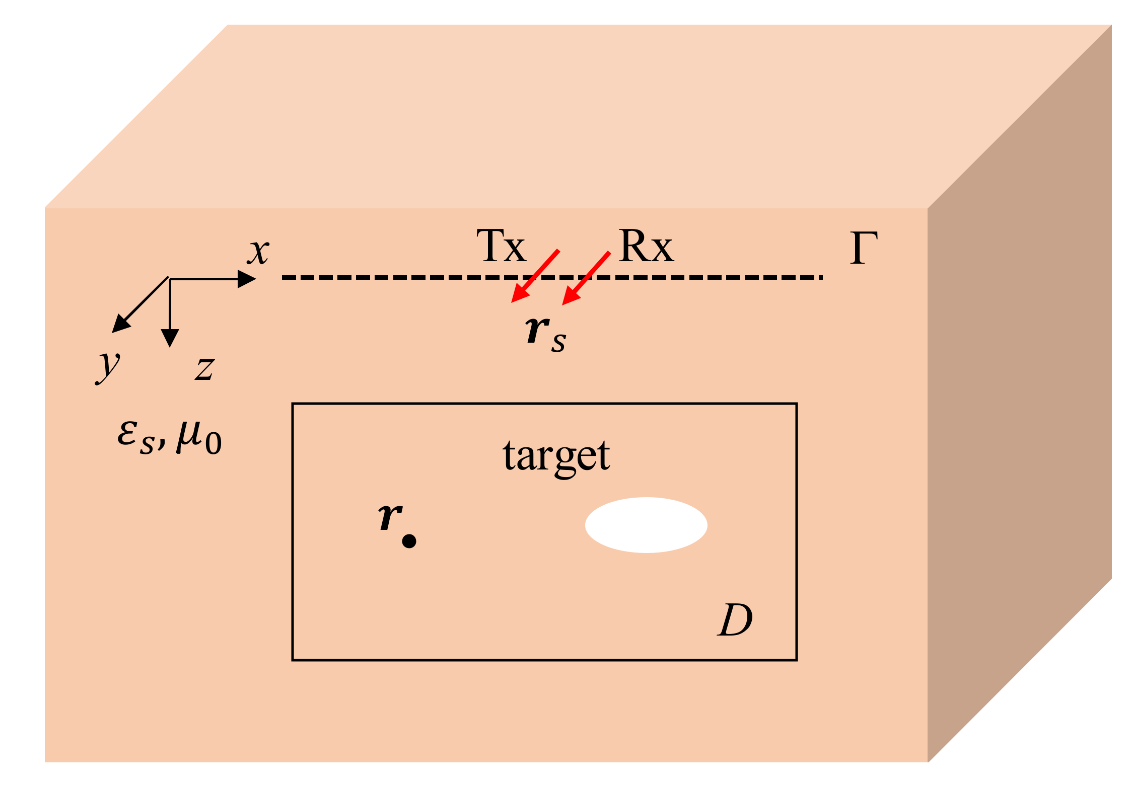
This section describes the mathematical models at the basis of the linear MWI approach. The models refer to the scenario in Figure 1 where the hosting medium is lossless, homogenous, non-magnetic, and characterized by the dielectric permittivity ${\epsilon }_s$ and magnetic permeability ${\mu }_0=4\pi \times {10}^{-7}$ H/m. The targets are probed by a Tx/Rx antenna pair moving along the line Γ at $z$= 0. The antennas collect data in the angular frequency range $\mathsf{\Omega }=\left[{\omega }_{min},{\omega }_{max}\right]$ and operate in monostatic mode; therefore, the generic measurement position is denoted by ${\mathit{r}}_s\in \mathsf{\Gamma }$. In the following, the $\exp \left(j\omega t\right)$ time dependence is assumed and dropped.

The investigation domain $D$ is a rectangular region hosting the targets identified by the survey direction (x-axis) and z-axis. Without loss of generality, it is assumed that the measurement line $\mathsf{\Gamma }$ and the investigation domain $D$ are both located at $y=y_s=0$ (see Figure 1). Therefore, it follows that ${\mathit{r}}_s=x_s\widehat{x}$ and $\mathit{r}=x\widehat{x}+z\widehat{z}$.

At any point $\mathit{r}\in D$, the presence of a target is described by the contrast function $\chi ={\epsilon }_t/{\epsilon }_s-1$, which represents the variation in the target permittivity ${\epsilon }_t$ with respect to the medium one ${\epsilon }_s$.

2.1. Full-3D Scattering Model

The antennas in Figure 1 are modeled as Hertzian dipoles linearly polarized in the direction normal to the survey line (y-axis). Under the Born approximation, the y-component of the scattered field $E_s^{3d}$ measured at ${\mathit{r}}_s$ is related to the unknown contrast function $\chi$ by the linear integral equation:

$$E_s^{3d}\left({\mathit{r}}_s,\omega \right)=\widehat{y}·k_s^2{\iint }_D^{}\underset{¯}{\underset{\_}{\mathit{G}}}\left({\mathit{r}}_s,\mathit{r}\right)·{\mathbf{E}}_i\left(\mathit{r},{\mathit{r}}_s\right)\chi \left(\mathit{r}\right)d\mathit{r}$$

(1)

where $k_s=\omega \sqrt{{\mu }_0{\epsilon }_s}$ is the propagation constant in the hosting medium, $\underset{¯}{\underset{\_}{\mathit{G}}}$is the dyadic Green’s function and ${\mathbf{E}}_i$is the incident electric field at $\mathit{r}$ radiated by a y-directed Hertzian dipole at ${\mathit{r}}_s$. The incident field ${\mathbf{E}}_i$is related to the dyadic Green’s function $\underset{¯}{\underset{\_}{\mathit{G}}}$by the formula [4]

$${\mathit{E}}_i\left(\mathit{r},{\mathit{r}}_s\right)=-j\omega {\mu }_0{I}_{0}l \underset{¯}{\underset{\_}{\mathit{G}}}\left(\mathit{r},{\mathit{r}}_s\right)·\widehat{y},$$

(2)

$I_{0}l$ being the electric dipole moment amplitude. The dyadic Green’s function $\underset{¯}{\underset{\_}{\mathit{G}}}$in a homogeneous and isotropic medium has a closed expression in the spatial domain [27] and, for the case at hand where $y=y_s=0$, the following expression holds:

$$\underset{¯}{\underset{\_}{\mathit{G}}}\left(\mathit{r},{\mathit{r}}_s\right)=\left[\begin{array}{ccc}{G}_1+G_2{\left(x-x_s\right)}^2& 0& G_2\left(x-x_s\right)z\\ 0& G_1& 0\\ G_2\left(x-x_s\right)z& 0& G_1+G_2{z}^2\end{array}\right]e^{-j{k}_s\mathit{R}}$$

(3)

$$G_1=\frac{-1-j{k}_{s}R+k_s^2{R}^2}{4\pi k_s^2{R}^3}$$

(4)

$$G_2=\frac{3+j3k_{s}R-k_s^2{R}^2}{4\pi k_s^2{R}^5}$$

(5)

where $R=\left|\mathit{r}-{\mathit{r}}_{\mathbf{s}}\right|=\sqrt{{\left(x-x_s\right)}^2+z^2}$.

Upon accounting for Equations (2)–(5), Equation (1) can be rewritten as

$$E_s^{3d}\left({\mathit{r}}_s,\omega \right)=-j\omega {\mu }_0{I}_{0}l{\iint }_D^{}{\left(\frac{-1-j{k}_s\mathit{r}+k_s^2{\mathit{r}}^2}{4\pi k_s{\mathit{r}}^3}\right)}^2{e}^{-j2k_s\mathit{r}}\chi \left(\mathit{r}\right)d\mathit{r}$$

(6)

The last formula is rewritten by introducing the compact operator notation as

$$E_s^{3d}={\mathcal{A}}^{3d}\chi$$

(7)

where ${\mathcal{A}}^{3d}$: ${\mathcal{L}}^2\left(D\right)\to {\mathcal{L}}^2\left(\mathsf{\Gamma }\times \mathsf{\Omega }\right)$ is a linear operator mapping the unknown space into the data space and ${\mathcal{L}}^2$ denotes the square integrable function space.

2.2. 2D Scattering Model

A common hypothesis adopted in MWI literature is to assume the invariance of the scene in the direction perpendicular to the image plane (i.e., y-direction in Figure 1) and model the antennas as filamentary electric currents directed along y (TM polarization) with amplitude I. Under these assumptions, the following scalar integral equation holds:

$$E_s^{2d}\left({\mathit{r}}_m,\omega \right)=k_{s }^2{{\displaystyle \iint }}_D^{}G\left({\mathit{r}}_s,\mathit{r}\right)E_i\left(\mathit{r},{\mathit{r}}_s\right)\chi \left(\mathit{r}\right)d\mathit{r}$$

(8)

where

$$G\left({\mathit{r}}_s,\mathit{r}\right)=\frac{j}{4}{H}_0^{\left(2\right)}\left(k_s\left|\mathit{r}-{\mathit{r}}_s\right|\right)$$

(9)

is the 2D Green’s function and $H_0^{\left(2\right)}$ is the Hankel’s function of second kind and zero order. Since

$$E_i\left(\mathit{r},{\mathit{r}}_s\right)=-j\omega {\mu }_{0}IG\left({\mathit{r}}_s,\mathit{r}\right),$$

(10)

and accounting for the reciprocity of Green’s function [4], the integral equation in (8) is rewritten as

$$E_s^{2d}\left({\mathit{r}}_m,\omega \right)=\frac{\omega {\mu }_{0}I{k}_{s }^2}{16}{{\displaystyle \iint }}_D^{}{\left(H_0^{\left(2\right)}\left(k_{s}R\right)\right)}^2\chi \left(\mathit{r}\right)d\mathit{r}$$

(11)

Similar to the 3D model in Section 2.1, the last equation is rewritten by using the operator notation

$$E_s^{2d}={\mathcal{A}}^{2d}\chi$$

(12)

where ${\mathcal{A}}^{2d}$: ${\mathcal{L}}^2\left(D\right)\to {\mathcal{L}}^2\left(\mathsf{\Gamma }\times \mathsf{\Omega }\right)$ is the 2D linear scattering operator.

2.3. Far-Field Operators

In this subsection, we present the far-field approximations of the 3D and 2D operators defined by Equations (6) and (11), respectively. The reason for introducing them is that they allow the geometrical attenuation term to be factorized, which can be then separated from the remaining amplitude terms. In Section 3.2, the SVD of the far-field operators is studied to highlight the role of the amplitude term while comparing the resolution performance of the 3D and 2D scattering models.

In the far-field approximation, the distance $R$ is large in terms of the EM wavelength, i.e., $k_{s}R\gg 1$. As a consequence, it is straightforward to verify that Equation (6) rewrites as

$$E_s^{3d}\left({\mathit{r}}_s,\omega \right)\approx \frac{-j\omega {\mu }_0{k}_s^2{I}_{0}l}{16{\pi }^2}{{\displaystyle \iint }}_D^{}\frac{e^{-j2k_s\mathit{r}}}{R^2}\chi \left(\mathit{r}\right)d\mathit{r}$$

(13)

As regards 2D model, we exploit the asymptotic form of the Hankel’s function [27]

$$H_0^{\left(2\right)}\left(z\right)\approx \sqrt{\frac{2}{\pi z}}{e}^{-j\left(z-\frac{\pi }{4}\right)}$$

(14)

which allows rewriting Equation (11) as

$$E_s^{2d}\left({\mathit{r}}_m,\omega \right)\approx \frac{j\omega {\mu }_{0}I{k}_s}{8\pi }{{\displaystyle \iint }}_D^{}\frac{e^{-j2k_{s}R}}{\mathit{r}}\chi \left(\mathit{r}\right)d\mathit{r}$$

(15)

Note that, in Equations (13) and (15), the geometrical attenuation factors $1/R^2$ and $1/R$, respectively, are factorized unlike Equations (6) and (11).

A further simplification, which will be exploited later in Section 3.2, is to neglect all the amplitude terms outside the integral in Equations (13) and (15), thus obtaining the simple integral relationships

$$E_s^{3d}\left({\mathit{r}}_s,\omega \right)\approx {{\displaystyle \iint }}_D^{}\frac{e^{-j2k_{s}R}}{R^2}\chi \left(\mathit{r}\right)d\mathit{r}$$

(16)

$$E_s^{2d}\left({\mathit{r}}_m,\omega \right)\approx {{\displaystyle \iint }}_D^{}\frac{e^{-j2k_{s}R}}{R}\chi \left(\mathit{r}\right)d\mathit{r}$$

(17)

We recall that only a qualitative image (i.e., the support) of the target can be retrieved by inverting a linear scattering model and the phase term plays the main role in the imaging process. In this respect, the approximate models of Equations (16) and (17) are admissible because the phase term is the same as in Equations (13) and (15).

2.4. The Solution of the Inverse Problem

The inverse problem is discretized by applying the Method of Moments [27], thus obtaining the matrix equation

$$E_s=\underset{¯}{\underset{\_}{A}}\cdot \chi$$

(18)

where $E_s\in {ℂ}^M$ and $\chi \in {ℂ}^N$ are the complex data and unknown vectors, respectively, and $\underset{¯}{\underset{\_}{A}}\in {ℂ}^{M\times N}$ is the matrix representing the scattering operator. Note that the matrix $\underset{¯}{\underset{\_}{A}}$ has rank $p\le \min \left(M,N\right)$.

The matrix $\underset{¯}{\underset{\_}{A}}$ is ill conditioned since it comes from the discretization of an ill-posed linear inverse problem [23]. Accordingly, the presence of noise on data makes the inversion an unstable process and it is necessary to apply a regularization scheme to get a physically meaningful solution. To this aim, we apply the Truncated Singular Value Decomposition (TSVD) strategy [23]

$$\tilde{\chi }={\displaystyle \sum }_{n=1}^{N_t}\frac{E_{\mathrm{s}}\cdot u_n^H}{{\sigma }_n}{v}_n$$

(19)

in which the superscript H is the conjugate transpose operation, ${\left\{{\sigma }_n,u_n,v_n\right\}}_{ }$ is the singular system of the relevant 3D/2D scattering operator matrix, ${\sigma }_n$ are singular values ordered in a descending order, $u_n$ and $v_n$ are orthonormal basis vectors in the space of data and unknowns, respectively. It is timely to remark that vectors $u_n$ depend on the measurement point $x_s$ while vectors $v_n$ depend on the point (x, z) in $D$. The regularization parameter $N_t$ is the number of retained singular values and its value is fixed in such a way to find an optimal trade-off between the accuracy and stability of the solution. In this work, as shown in Section 3, $N_t$ is determined according to the L-curve method [28].

The modulus of the retrieved contrast vector $\tilde{\chi }$ defines a spatial map herein referred to as tomographic image.

2.5. Point Spread Function and Spectral Content

The resolution analysis is herein carried out by considering two different figures of merit. The first one is the PSF, which is the regularized reconstruction of a point target [23]. Scattered field data are generated according to the 3D model being the data always referred to a 3D scenario in real applications; hence, the imaging is faced by exploiting both the 3D and 2D models and it is solved as described in Section 2.4.

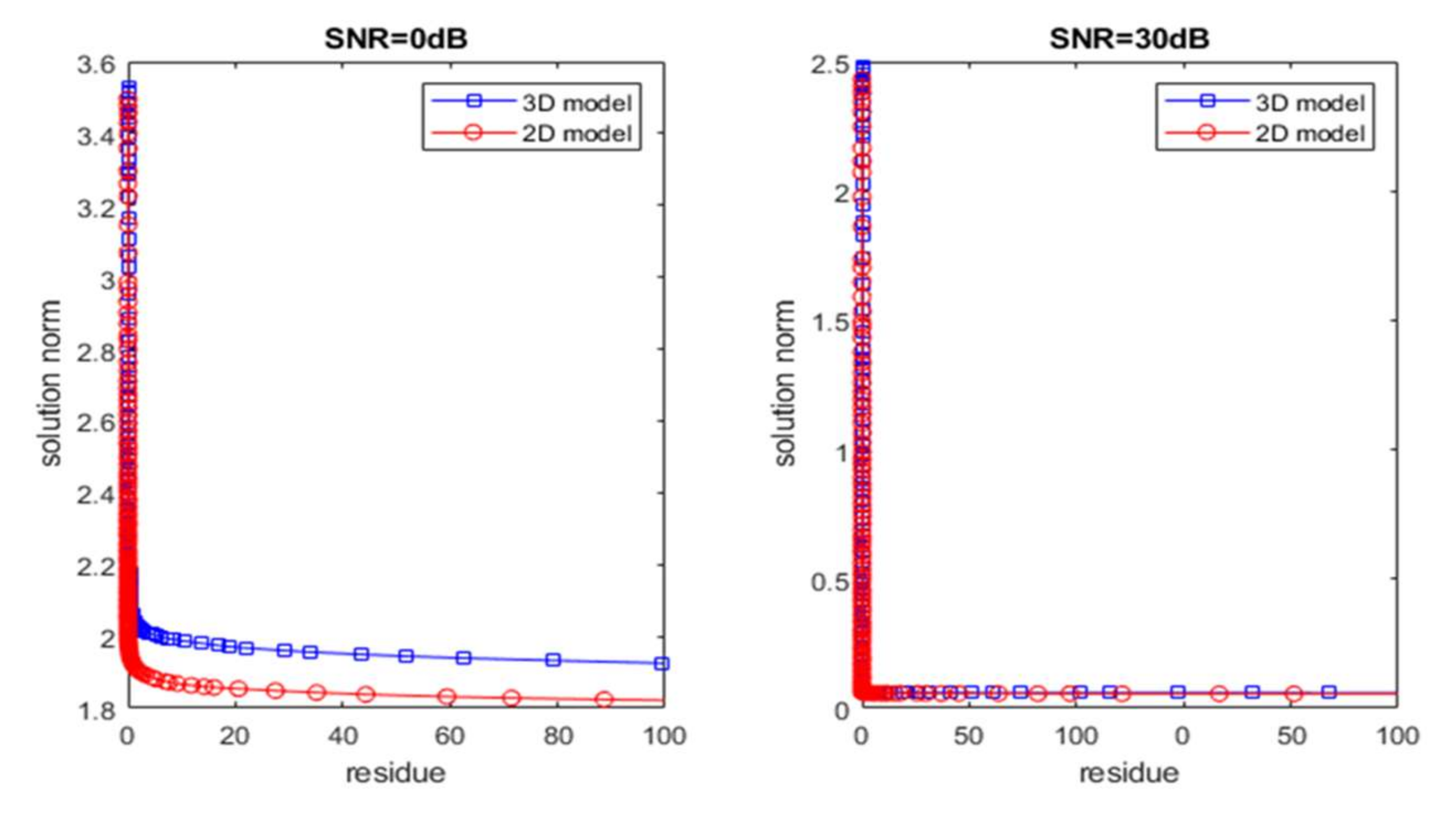
The matrix $\underset{¯}{\underset{\_}{A}}$ in Equation (18) represents the discretized version of the scattering operator ${\mathcal{A}}^{3d}$ when the 3D model is adopted and of ${\mathcal{A}}^{2d}$ in the 2D case. The data are corrupted by Additive White Gaussian Noise (AWGN) with a specified signal noise ratio (SNR) level. Then, the comparison of 3D and 2D models is performed at parity of SNR. Specifically, for a fixed SNR level, data are inverted according to the TSVD strategy of Equation (19) where the regularization parameter $N_t$ is evaluated automatically according to the L-curve criterion. The L-curve is a log–log plot of the norm of the regularized contrast ${\Vert \chi \Vert }^2$versus the norm of the corresponding residue ${\Vert E_s-\underset{¯}{\underset{\_}{A}}\cdot \chi \Vert }^2$. The optimal $N_t$ value is the one achieved in correspondence of the corner of the L-curve [28].

The second figure of merit adopted here to compare the considered scattering models is the spectral content of the scattering operators [19,21,22,24]. This quantity allows visualizing the retrievable spectral components of the unknown contrast function. Note that, differently from PSF, the spectral content provides a global information related to the considered investigation domain rather than information at a specific target location. When the TSVD inversion scheme is adopted, the spectral content is defined as the sum of the square amplitude of the discrete Fourier transforms of the singular vectors $v_{\mathrm{n}}$ corresponding to the retained singular values, i.e.,

$$SC\left(k_x,k_z\right)={{\displaystyle \sum }}_{n=1}^{N_t}{\left|{\tilde{\mathbf{v}}}_n\left(k_x,k_z\right)\right|}^2$$

(20)

where $k_x,k_z$ are the spectral variables corresponding to $x,z$ and ${\tilde{v}}_n\left(k_x,k_z\right)$ are the 2D discrete Fourier transforms of the singular vectors $v_n.$ An interpretation relating the spectral content to the Fourier transform of the PSF has been reported in [25].

3. Resolution Analysis for 3D and 2D Models

3.1. Scenario Description

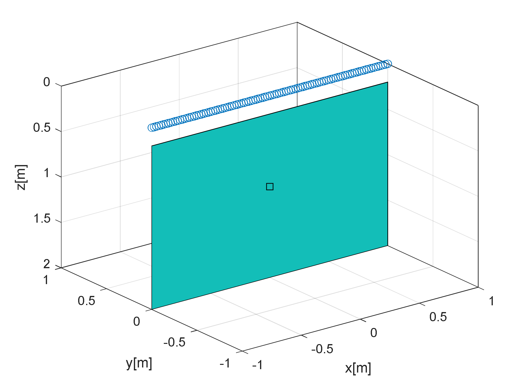
The resolution analysis of the 3D and 2D scattering models is carried out for the scenario depicted in Figure 2. The measurement domain $\mathsf{\Gamma }$ is a 2 m long line directed along the $x$-axis covering the interval [−1.0, 1.0] m and sampled with a step equal to 0.02 m. The investigation domain is the rectangle $D$ = [−1.0, 1.0] $\times$ [0.2, 2.0] m² in the x-z plane discretized into square image pixels with side 0.02 m. A lossless homogeneous and non-magnetic dielectric medium having a dielectric permittivity ${\epsilon }_s=4{\epsilon }_0$, ${\epsilon }_0$ = 8.85 × 10⁻¹² F/m being the free-space permittivity, is considered. The point target is buried 1 m below the measurement line at (0, 0, 1) m. The currents $I_0$ and $I$ involved in Equations (6) and (11) are assumed equal to 1 A and the dipole length is $l=$ 0.001 m.

The scattered field data are computed according to the 3D scattering model over the frequency range from 500 to 1500 MHz with a step of 30 MHz. The considered band covers frequencies commonly used in MWI, and allows simulating a MWI system operating with 1 GHz center frequency. On the other hand, the proposed methodology is general and applicable as it is in other frequency bands. Each trace of the frequency domain data set is corrupted by AWGN with progressively increasing SNR levels going from 0 to 30 dB with a step of 5 dB.

3.2. Singular Values Analysis and Optimal Truncation Index

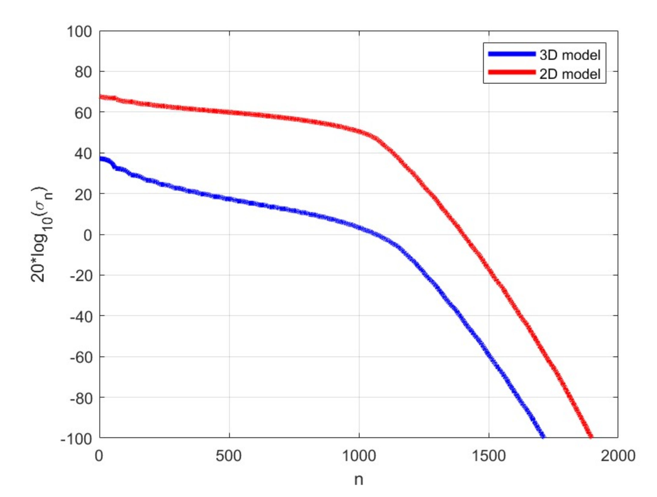
Figure 3 displays the curves of the singular values of the 3D and 2D scattering operators on a dB scale. As can be seen, both curves exhibit a progressive decay of the singular values as the index $n$ grows; a more significant decay is observed for the 3D model (blue curve) compared to the 2D one (red curve). Most notably, the singular values of the 2D model are significantly higher (at least one order of magnitude) than those of the 3D model for every index n.

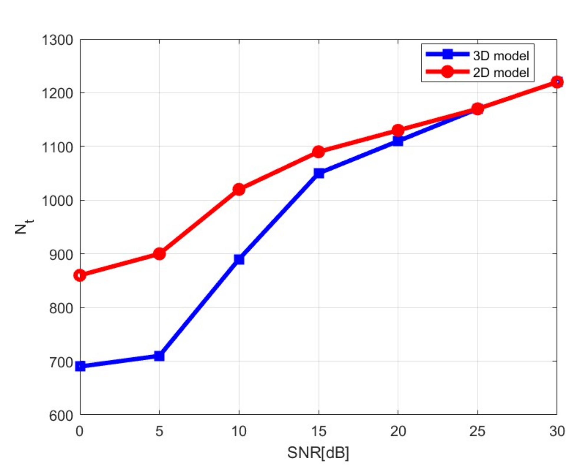
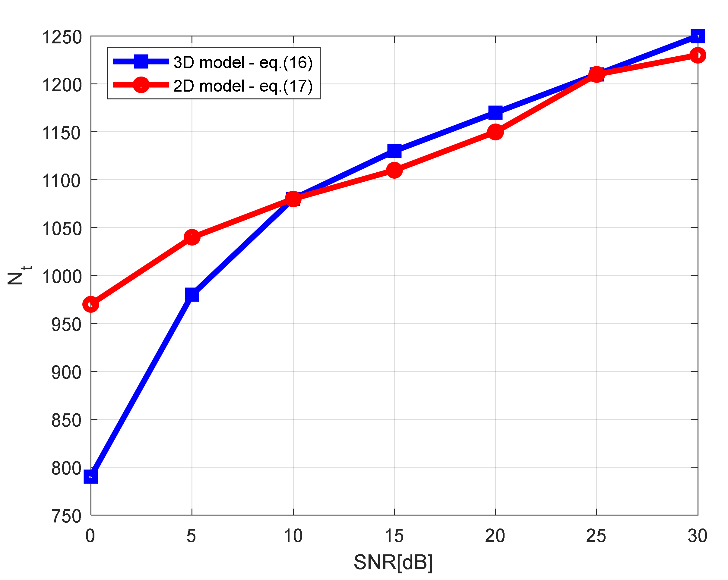
The resolution performance that is achievable with the two models depends on the truncation index $N_t$ and, in turn, on the SNR level. In this respect, Figure 4 shows the optimal $N_t$ value versus SNR achieved with the 3D and 2D models after applying the L-curve method. In the low SNR region, the $N_t$ value, i.e., the number of retained singular values, is significantly lower for 3D model compared to the 2D model one. On the other hand, at high SNRs, $N_t$ values are very similar for both models. This suggests different performance of the models when data are severely corrupted by noise, and such a behavior depends on the different amplitudes of the singular values formerly observed in Figure 3. As a result, a worse performance in terms of spatial resolution limits is expected for the 3D model at low SNRs.

For sake of clarity, we report in Figure 5 the L-curves attained for 3D and 2D models when SNR = 0 dB (left panel) and 30 dB (right panel). As can be observed, the 2D model is generally characterized by a lower norm of the solution when SNR = 0 dB.

In order to investigate more in detail, the role played by the level of the singular values on the robustness of the solution with respect to the noise, and so in determining the optimal $N_t$ value, it is useful to consider the expressions of the residue and the norm of the regularized contrast (see Appendix A):

$${\Vert E_s-\underset{¯}{\underset{\_}{A}}\cdot \tilde{\chi }\Vert }^2={{\displaystyle \sum }}_{n=N_t+1}^p{\left|{\tilde{E}}_s\cdot u_n^H\right|}^2+{{\displaystyle \sum }}_{n=N_t+1}^p{\left|w\cdot u_n^H\right|}^2+{{\displaystyle \sum }}_{n=N_t+1}^{p}2\mathrm{Re}\left\{\left({\tilde{E}}_s\cdot u_n^H\right){\left(w\cdot u_n^H\right)}^{*}\right\}$$

(21)

$${\Vert \tilde{\chi }\Vert }^2={{\displaystyle \sum }}_{n=1}^{N_t}\frac{{\left|{\tilde{E}}_s\cdot u_n^H\right|}^2}{{\sigma }_n^2}+{{\displaystyle \sum }}_{n=1}^{N_t}\frac{{\left|w\cdot u_n^H\right|}^2}{{\sigma }_n^2}+{{\displaystyle \sum }}_{n=1}^{N_t}\frac{2\mathrm{Re}\left\{\left({\tilde{E}}_s\cdot u_n^H\right){\left(w\cdot u_n^H\right)}^{*}\right\}}{{\sigma }_n^2}$$

(22)

where ${\tilde{E}}_s$ is the noiseless scattered field and $w$ is the AWGN vector.

Both residue and norm in Equations (21) and (22) are the superposition of three series where the first two are positive quantities and the third one can assume positive or negative values depending on the signs of the scalar products.

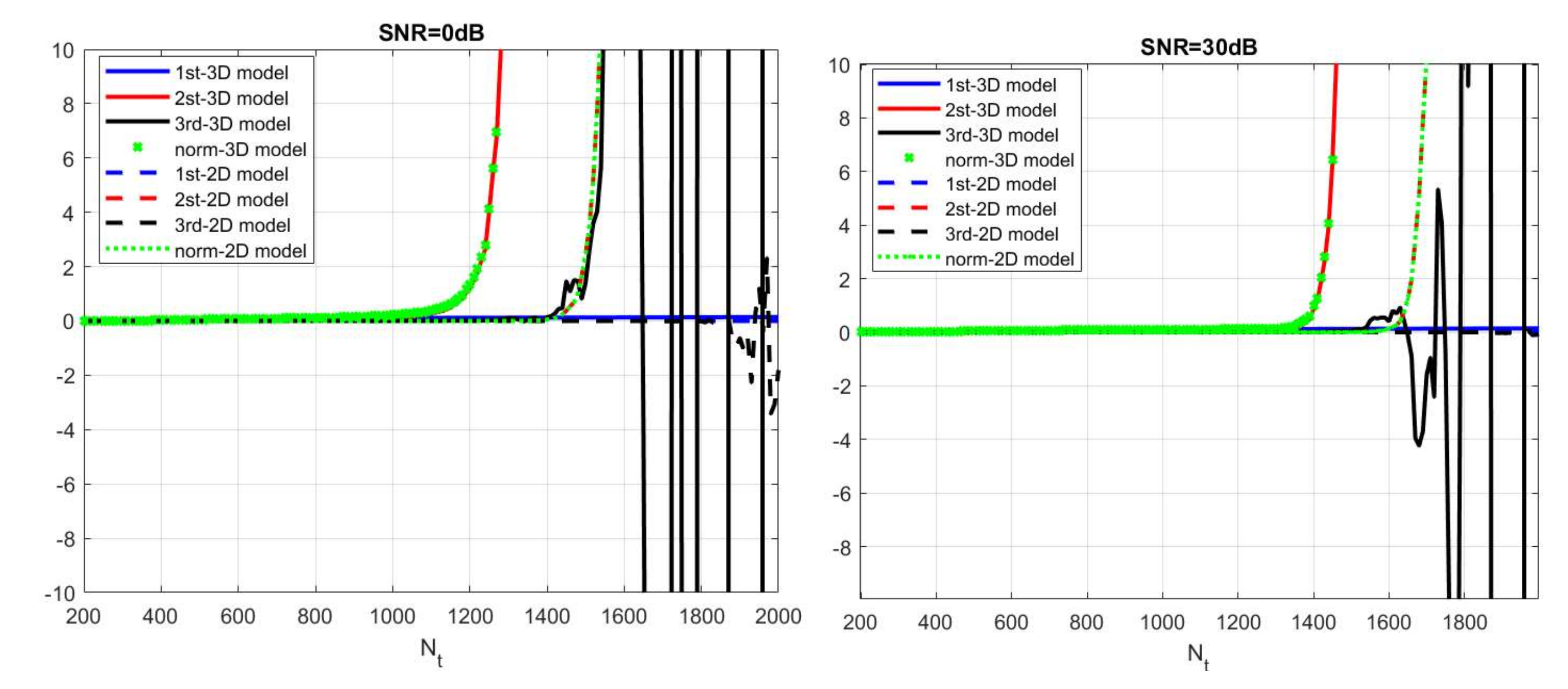
The graphs depicted in Figure 6 show the three terms of Equation (21) and the residue versus $N_t$ for 3D and 2D models when SNR = 0 dB (left panel) and SNR = 30 dB (right panel). In general, it is observed that the residue is finite and decays with increasing $N_t$. Moreover, the two models have similar behavior of residue.

The graphs in Figure 7 are concerned with the norm of the solution (see Equation (22)) for SNR = 0 dB (left panel) and SNR = 30 dB (right panel). All the three terms involved in Equation (21) are also reported for clarity. As discussed in Appendix A, the first term (blue curves) is limited for every $N_t$ in agreement with the Discrete Picard Condition [29]. On the other hand, the second term (red curves) is divergent and essentially determines the behavior of the norm (green curves) as $N_t$ grows. In particular, for 3D model, the second term starts to diverge at a smaller $N_t$ compared to the one of the 2D model. The third term (black curves) has an oscillating trend that does not play a meaningful role on the norm of the solution. In view of the finite values of the residue, it turns out that the optimal $N_t$ (L-curve corner) is mainly influenced by the divergent behavior of the norm of the solution. Regardless of the noise level, the norm of the solution for the 3D model starts to diverge before the one associated with the 2D model, and this justifies the difference in $N_t$ values observed in Figure 4.

3.3. Point Spread Function and Spectral Content

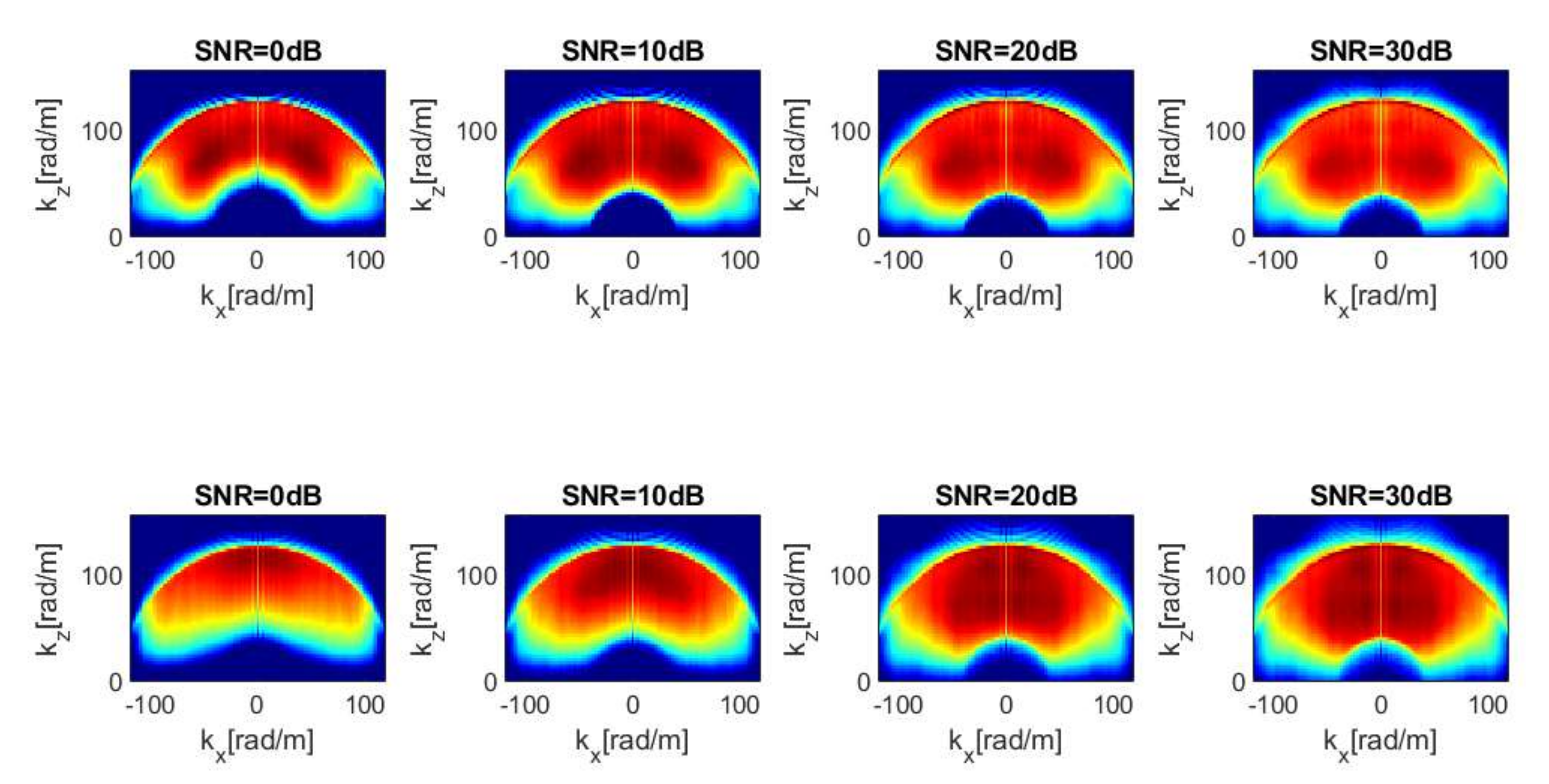
The imaging performance of the considered models is assessed in Figure 8 in terms of spectral contents. These last are evaluated via Equation (20) by setting the TSVD truncation index in accordance with the curves reported in Figure 4. The spectral contents of both models are characterized by a low-pass filtering along the x-axis and a band-pass filtering along z. Moreover, the comparison of the spectral contents provides similar trends for the two models save for low SNR values. Indeed, at low SNR, the spectral content of the 3D model (lower panels) exhibits a more severe filtering along the z-axis, i.e., a bandwidth reduction. The spatial filtering here shown is typical for an electromagnetic inverse scattering problem when an aspect limited reflection configuration is exploited (e.g., see [19]).

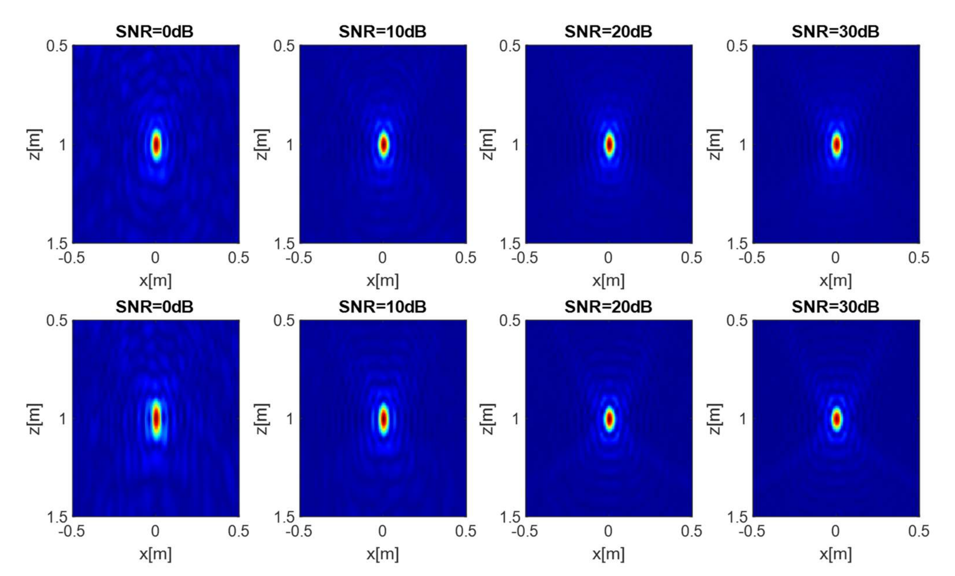
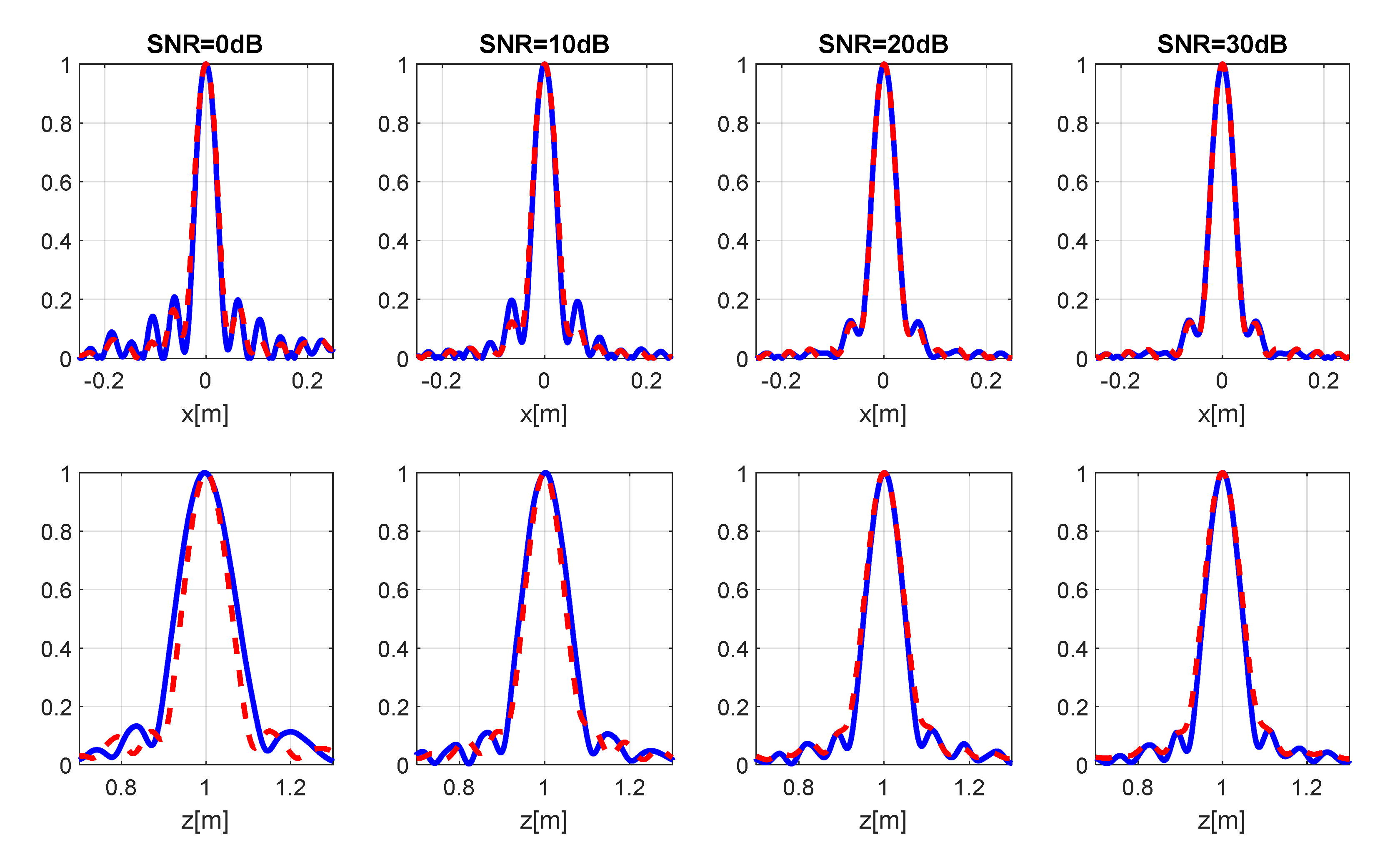
The images plotted in Figure 9 show the normalized amplitude of the regularized PSF for 2D (upper panels) and 3D (lower panels) models versus SNR, achieved in correspondence of the optimal truncation indexes shown in Figure 4; in particular, SNR = 0, 10, 20, 30 dB values are considered for sake of brevity. As expected, the PSFs are characterized by a focused spot in correspondence of the target position. Notably, the main lobe width along the x-axis turns out to be almost independent on the SNR on the data for both models. On the other hand, the lobe width along z-axis for the 3D model appears slightly larger compared to the 2D model one as the SNR level decreases. This phenomenon is better highlighted by the cuts of the PSF reported in Figure 10.

In order to provide a more quantitative assessment of the imaging performance,

Table 1. Resolution for a point target at (0,0,1) m.

	3D Model			2D Model
SNR (dB)	Δx (cm)	Δz (cm)	Nt	Δx (cm)	Δz (cm)	Nt
0	3.8	11.2	690	3.8	9.0	860
5	3.8	10.1	710	3.8	8.2	900
10	3.8	8.9	890	3.8	7.6	1020
15	3.8	8.1	1050	3.8	7.6	1090
20	3.8	7.6	1110	3.8	7.6	1130
25	3.8	7.6	1170	3.8	7.6	1170
30	3.8	7.6	1220	3.8	7.6	1220

summarizes the resolution limits and the optimal truncation index for each model and SNR level. Note that the spatial resolution $(\mathsf{\Delta }x$ and $\mathsf{\Delta }z$) is evaluated according to the full-width at half-maximum (FWHM) of the PSF main lobe. The reason for such choice is that, as revealed by Figure 10, the PSF cuts do not always have definite nulls close to the main lobe, and therefore it is not possible to apply reliably the usual Rayleigh criterion [23].

Numerical data in Table 1 confirm that resolution along z worsens when the data are noisy and the most notable deterioration arises with the 3D model. On the other hand, no resolution variation is observed along the $x$-axis coherently with the qualitative PSF analysis (see Figure 9 and Figure 10).

In the following, we also analyze the effect of the target position on the resolution limits. Specifically, the aim is to investigate how the PSF changes when the target is located at different distances, i.e., at z = 0.5 m, z = 1 m, z = 1.5 m, with respect to the antennas. For this case, it has been found that 3D and 2D models provide similar imaging performance, save for the low SNR case. For sake of brevity, here we do not present the PSF reconstructions and report only the resolution data achieved when the SNR is equal to 0 dB (see

Table 2. Resolution for a point target at different distances from the antennas when SNR = 0 dB.

	3D Model			2D Model
Depth (m)	Δx (cm)	Δz (cm)	Nt	Δx (cm)	Δz (cm)	Nt
0.5	2.6	9.4	280	2.6	9.0	380
1	3.8	11.2	690	3.8	9.0	860
1.5	4.9	13.4	840	4.9	8.7	990

), which are those showing the major variations between the models. As can be seen, both models again exhibit identical resolutions along x-axis, which progressively worsen as the target depth increases due to the smaller illumination angle [19]. With regard to the resolution along z, as previously observed, a significant focusing enhancement is achieved by inverting the 2D model because a larger number of singular values is retained in the TSVD compared to the 3D model.

3.4. 3D vs. 2D Model: The Far-Field Case

In order to investigate in more detail the reason why the 3D model is less performing than the 2D one in the low SNR region, we compare in Figure 11 the curves of the singular values of 3D and 2D operators (Equations (6) and (11)) with those of their far-field approximations. Specifically, the magenta and green curves refer to the far-field operators accounting for all amplitude terms (Equations (13) and (15)), while the black and gray curves are related to the far-field operators where the geometrical spreading is the only amplitude term (Equations (16) and (17)). It is interesting to observe that the curves of the 3D and 2D operators and their corresponding far-field approximations containing all amplitude terms (Equations (13) and (15)) are identical. This means that the far-field condition holds for the considered investigation domain and operating frequency band. Most notably, we can also notice that the curves of the 3D and 2D far-field operators that do not contain amplitude terms outside the integrals (Equations (16) and (17)) are very similar each other and different from the remaining ones. This means that the amplitude factor not including the geometrical attenuation is the main reason why 3D and 2D operators containing all amplitude factors behave differently.

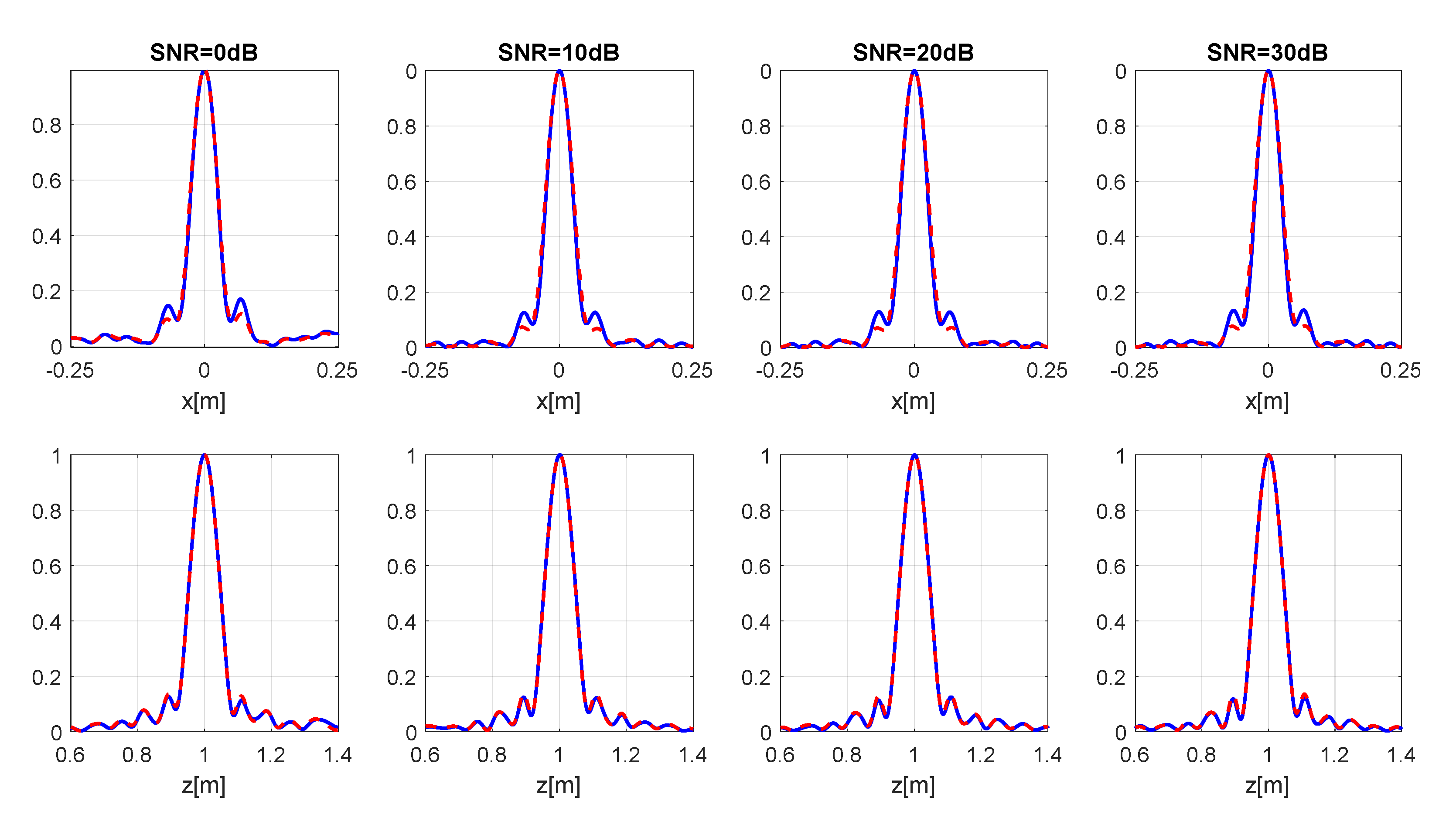
To support this claim, we report in Figure 12 the optimal regularization parameters and in Figure 13 the PSF cuts achieved by inverting the 3D and 2D far-field operators defined by Equations (16) and (17). As can be observed, unlike Figure 4, the optimal regularization parameters in this case look more similar and the PSF cuts of the 3D and 2D models match very well (see Figure 13).

4. Reconstruction Results

In this section, numerical experiments are reported to further assess the imaging performance of the 3D and 2D models in the case of extended targets. To this end, the full-wave electromagnetic solver GPRMAx3D [30] is exploited to generate synthetic data with transmitting dipoles radiating a Ricker wavelet centered at the frequency of 1.0 GHz. The simulation parameters of the implemented model such as medium properties, measurement configuration and investigation domain are identical to those previously considered for the resolution analysis in Section 3.

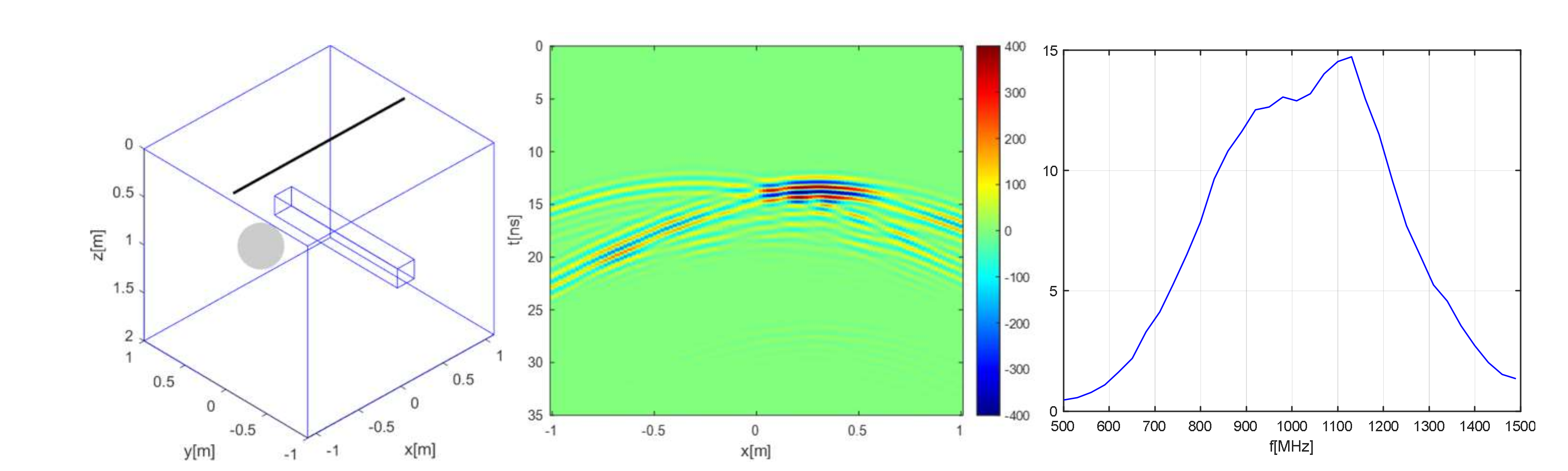
The first considered scenario is sketched in the left panel of Figure 14 and features a spherical cavity (${\mathsf{\epsilon }}_{\mathrm{t}}={\mathsf{\epsilon }}_0)$ centered at (0.0,0.0,1.2) m and having radius 0.2 m. The 2 m long measurement line at y = 0 is located 1.2 m exactly above the cavity center. Moreover, the investigation domain also passes through the center of the cavity virtually cutting it into two equal parts.

The simulated data are generated over the fast-time window (0, 35) ns and processed according to following operations: zero time setting at 1 ns and time-gating up to 13 ns to filter out the direct coupling between the Tx and Rx antennas. The filtered data so obtained (middle panel in Figure 14) account for the field scattered from the target, which appears in the typical form of a diffraction hyperbola [5]. Each trace of filtered data is transformed in the frequency domain over the band from 500 to 1500 MHz with a step of 30 MHz. The average spectrum of the noiseless scattered field data is represented in the right panel of Figure 14. Afterwards, each trace of the frequency domain data is corrupted by AWGN with progressively increasing SNR levels from 0 to 30 dB in 10 dB steps. For each SNR level, the frequency domain data are inverted according to the 3D and 2D models and the L-curve method is applied.

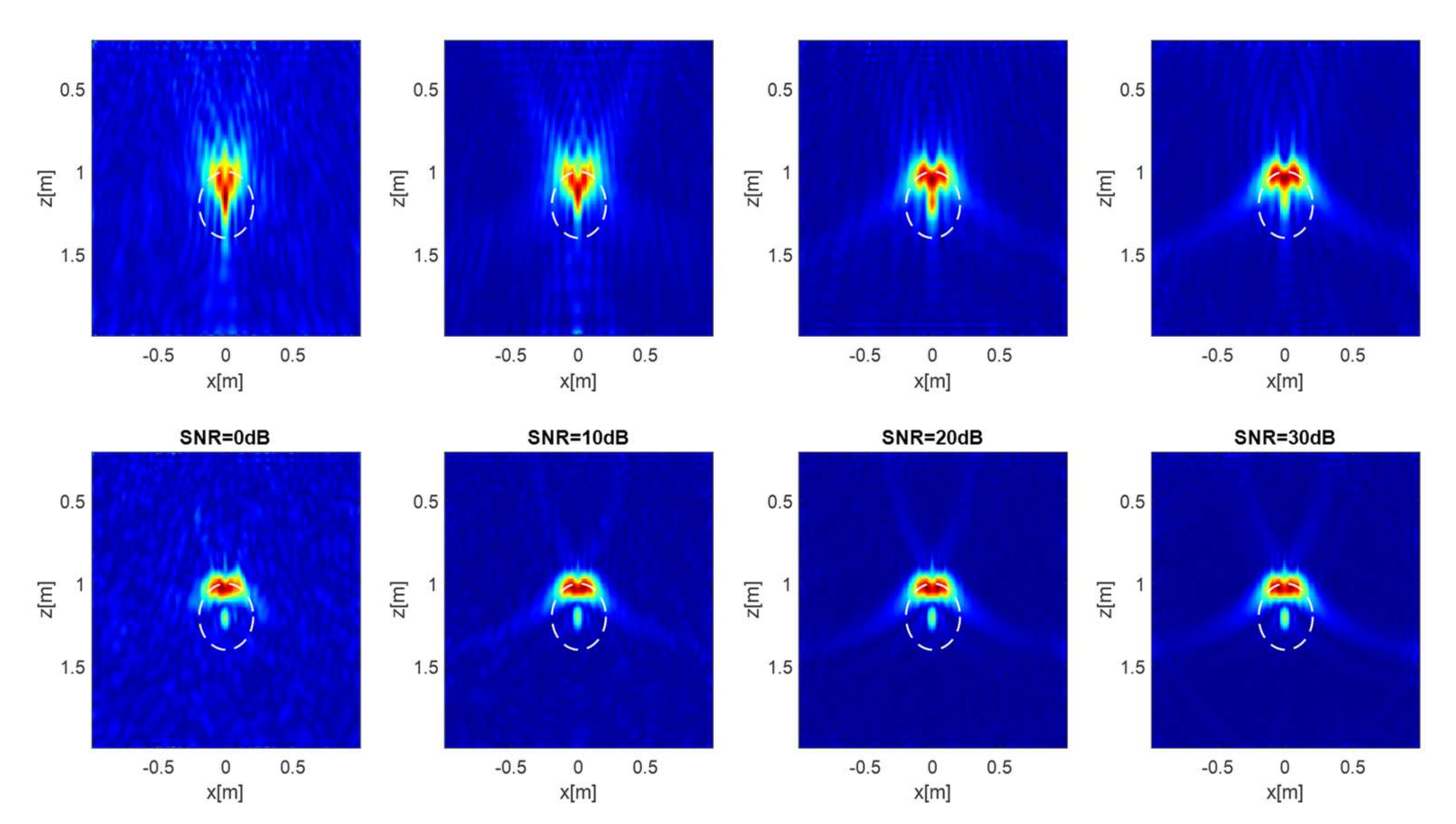
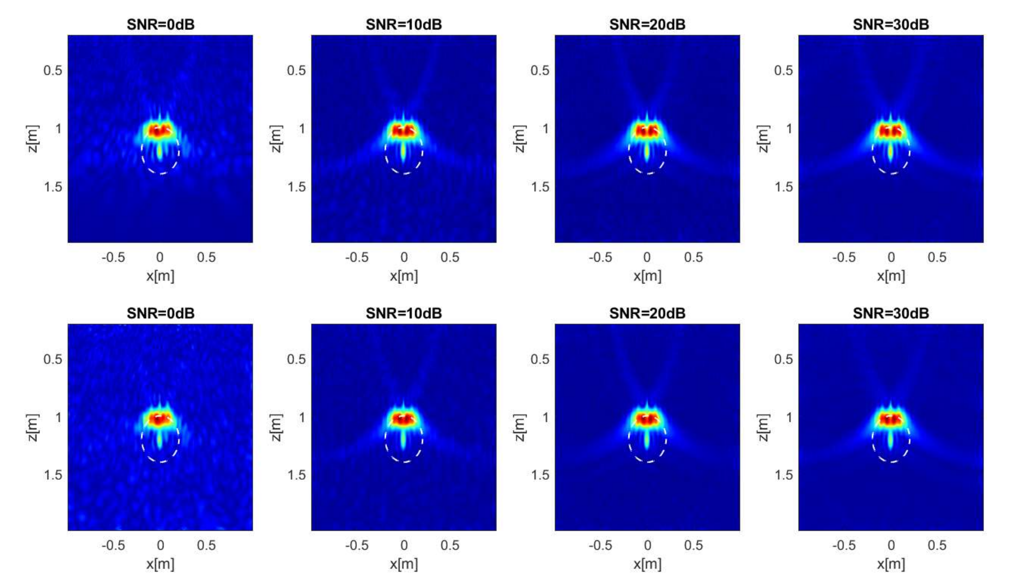
The images plotted in Figure 15 are the tomographic reconstructions related to the 3D (upper panels) and 2D (lower panels) models for the different SNR values. In general, each reconstruction is characterized by the presence of a well-focused spot along the upper target interface. Furthermore, the lower side of the target is clearly defocused and delocalized as confirmed by the presence of the spot located in proximity of the cavity center. This effect is a peculiar feature of the considered linear models, which assume propagation in a homogenous medium with relative permittivity equal to 4 (v = 15 cm/ns) and do not take into account the actual (lower) permittivity of the cavity (v = 30 cm/ns). As for the comparison between the two models, the images in Figure 15 confirm that very similar results are achieved except when SNR = 0 dB. In this case, as already predicted by the PSF analysis in Section 3.3, the 3D model is characterized by a worse resolution along z, and consequently it is not possible to distinguish the upper part of the target contour from the lower one.

A further numerical test case referred to a two-target scenario is considered and shown in the left panel of Figure 16. The first target is a parallelepiped cavity with length 1.5 m along y and having a square cross-section with side 0.2 m in the $x-z$ plane. The center of the parallepiped is located at (0.3, 0.0, 1.1) m. A spherical cavity with radius 0.2 m and center at (−0.3, 0.4, 1.1) m is buried in proximity of the parallelepiped.

Unlike the parallelepiped cavity, the investigation domain at y = 0 does not intercept any part of the spherical target, which is thus illuminated in side-looking mode by the antennas placed at y = 0.

The raw data are processed according to the time-domain operations considered for the previous test and the achieved filtered data are represented in the middle panel of Figure 16. This image reveals the presence of several targets’ signatures, which can be attributed to the direct reflections by the targets and to the mutual interactions between them. The average spectrum of the time-domain data is also plotted in the right panel of Figure 16 for sake of completeness.

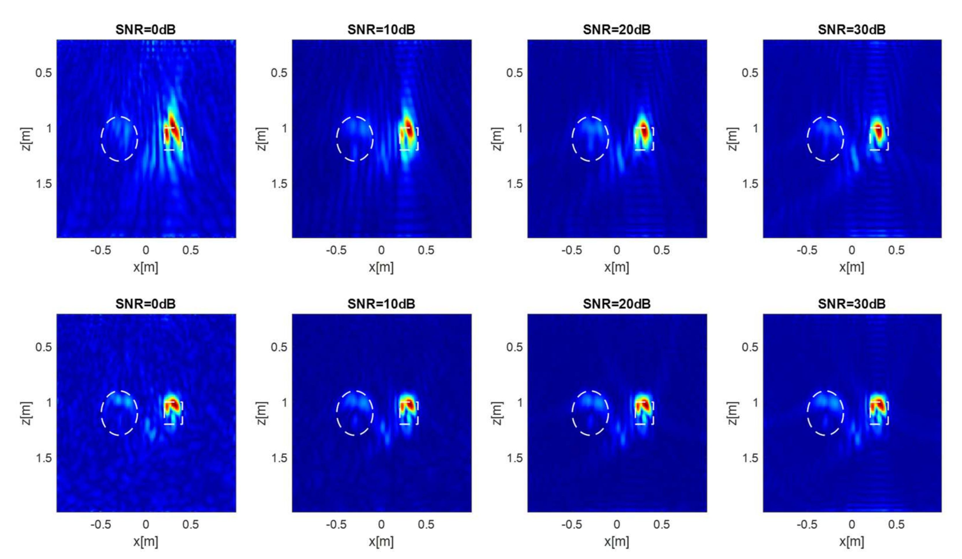
The tomographic reconstructions obtained by inverting the frequency domain data according to the 3D and 2D models are plotted in Figure 17. It is easily realized that this case is more challenging than the former one. The upper side of the parallelepiped is always clearly identified, as well as the lower edge, which is imaged in proximity of the target center. As regards the spherical cavity, the reconstruction of the upper contour is more attenuated with respect to the parallelepiped one because the sphere is illuminated laterally (with respect to the antenna radiation maximum) and so a weaker radar return is produced (see also filtered data in Figure 16). The upper edge of the sphere appears also slightly delocalized along z with a displacement of about 0.1 m with respect to the true target contour. This outcome is again due to the fact that the target is illuminated laterally and then the target range measured by the radar does not correspond to the distance along z. All reconstructions also highlight the presence of some artifacts produced by the interactions between the targets (multipath ghosts) that are not taken into account by the considered linear models [31,32]. Moreover, the superior resolution performance along z achieved by the 2D model at low SNRs is confirmed once again.

Finally, we show the tomographic reconstructions for the single-target (Figure 18) and two-targets (Figure 19) scenarios achieved by inverting the 3D and 2D far-field models of Equations (16) and (17). In this case, as already foreseen by the PSF analysis in Section 3.4, both models have similar imaging capabilities also at low SNR.

As regards the computational cost of the 3D and 2D imaging approaches,

Table 3. Computation times of the 3D and 2D inversion approach.

	3D Model	2D Model
Operator	5.34 s	5.14 s
SVD	50.2 s	51.3 s

summarizes the computation times (in seconds) to perform the data processing on a standard laptop equipped with an Intel(R) Core(TM) i7-8565U CPU and 16-GB RAM under MATLAB 2017 environment. As expected, both approaches have almost identical computation times because the matrices associated to the 3D and 2D operators have the same size M × N. In particular, the computational load is largely dominated by the SVD calculation whose processing time (about 50 s) is one order magnitude greater than the one required to evaluate the operator matrix (about 5 s). This result can be explained by considering that the operator matrix computation has complexity O(MN) while SVD has complexity O(k₁ M²N + k₂ N³), where k₁ and k₂ are some constants depending on the algorithm used [33].

5. Conclusions

This work has dealt with MWI and the achievable performance in the frame of the Born approximation when 3D and 2D scattering models are used to describe the data–unknown relationship. The presented analysis allows us to determine the best model to be inverted depending on the noise level of the data. A theoretical assessment of the achievable resolution was carried out accounting for the point spread function and the spectral content, which are two quantities commonly adopted to predict the imaging capabilities. Moreover, reconstructions results based on synthetic data referred to extended targets have been provided. For a fair comparison, the optimal regularization parameter was determined by applying the L-curve method.

The presented analysis has pointed out that when data are severely corrupted by noise, the inverse approach based on the 2D-scattering model turns out be slightly more effective in terms of robustness to noise and resolution along the direction perpendicular to the measurement line. Such an outcome is related to the higher singular values of the 2D operator, compared to the 3D ones, when all amplitude factors are accounted for in the scattering operator. However, for moderate to high SNRs, or if amplitude factors not including the geometrical attenuation term are neglected, the 3D and 2D models have almost identical performance.

Future research activities are concerned with the experimental verification of the theoretical analysis reported in this work, and the study of innovative measurement configurations, such as multiple lines and acquisition geometries different from the classical rectilinear one. Moreover, the conversion of the incident field from 3D to 2D, by a procedure similar to that reported in [26] in the seismic context, may be exploited to define a novel inverse scattering approach where the 2D Green’s function replaces the 3D Green’s function in the linear integral equation.

References

- Colton, D.; Kress, R. Inverse Acoustic and Electromagnetic Scattering Theory; Springer: New York, NY, USA, 1992. [Google Scholar]
- Pastorino, M. Microwave Imaging; Wiley: New York, NY, USA, 2010. [Google Scholar]
- Pastorino, M. Stochastic optimization methods applied to microwave imaging: A review. IEEE Trans. Ant. Propag. 2007, 55, 538–548. [Google Scholar] [CrossRef]
- Chew, W.C. Waves and Fields in Inhomogeneous Media; Institute of Electrical and Electronics Engineers: Piscataway, NJ, USA, 1995. [Google Scholar]
- Daniels, D.J. Ground Penetrating Radar; Institution of Engineering and Technology: London, UK, 2004. [Google Scholar]
- Davis, J.L.; Annan, A.P. Ground-penetrating radar for high-resolution mapping of soil and rock stratigraphy. Geophys. Prospect. 1989, 37, 531–551. [Google Scholar] [CrossRef]
- Benedetto, A.; Pajewski, L. Civil Engineering Applications of Ground Penetrating Radar; Springer: Berlin, Germany, 2015. [Google Scholar]
- Goodman, D.; Piro, S. GPR remote Sensing in Archaeology; Springer: New York, NY, USA, 2013. [Google Scholar]
- Capozzoli, L.; Catapano, I.; De Martino, G.; Gennarelli, G.; Ludeno, G.; Rizzo, E.; Soldovieri, F.; Uliano Scelza, F.; Zuchtriegel, G. The Discovery of a Buried Temple in Paestum: The Advantages of the Geophysical Multi-Sensor Application. Remote Sens. 2020, 12, 2711. [Google Scholar] [CrossRef]
- Catapano, I.; Gennarelli, G.; Ludeno, G.; Soldovieri, F. Applying ground-penetrating radar and microwave tomography data processing in cultural heritage: State of the art and future trends. IEEE Sign. Proc. Mag. 2019, 36, 53–61. [Google Scholar] [CrossRef]
- Fear, E.C.; Hagness, S.C.; Meaney, P.M.; Okoniewski, M.; Stuchly, M.A. Enhancing breast tumor detection with near-field imaging. IEEE Microw. Mag. 2002, 3, 48–56. [Google Scholar] [CrossRef]
- Nikolova, N.K. Microwave imaging for breast cancer. IEEE Microw. Mag. 2011, 12, 78–94. [Google Scholar] [CrossRef]
- Zoughi, R. Microwave Non-Destructive Testing and Evaluation; Kluwer: Norwell, MA, USA, 2000. [Google Scholar]
- Amin, M.G. Through-the-Wall Radar Imaging; CRC Press: Boca Raton, FL, USA, 2017. [Google Scholar]
- Randazzo, A.; Ponti, C.; Fedeli, A.; Estatico, C.; D’Atanasio, P.; Pastorino, M.; Schettini, G.A. Through-the-Wall Imaging Approach Based on a TSVD/Variable-Exponent Lebesgue-Space Method. Remote Sens. 2021, 13, 2028. [Google Scholar] [CrossRef]
- Gennarelli, G.; Soldovieri, F. A linear inverse scattering algorithm for radar imaging in multipath environments. IEEE Geosci. Remote Sens. Lett. 2013, 10, 1085–1089. [Google Scholar] [CrossRef]
- Gennarelli, G.; Amin, M.G.; Soldovieri, F.; Solimene, R. Passive multiarray image fusion for RF tomography by opportunistic sources. IEEE Geosci. Remote Sens. Lett. 2014, 12, 641–645. [Google Scholar] [CrossRef]
- Devaney, A.J. Geophysical diffraction tomography. IEEE Trans. Geosci. Remote. Sens. 1984, 1, 3–13. [Google Scholar] [CrossRef]
- Persico, R. Introduction to Ground Penetrating Radar: Inverse Scattering and Data Processing; John Wiley & Sons: Hoboken, NJ, USA, 2014. [Google Scholar]
- Chen, X. Computational Methods for Electromagnetic Inverse Scattering; John Wiley & Sons: Hoboken, NJ, USA, 2018. [Google Scholar]
- Ludeno, G.; Gennarelli, G.; Lambot, S.; Soldovieri, F.; Catapano, I. A comparison of linear inverse scattering models for contactless GPR imaging. IEEE Trans. Geosci. Remote. Sens. 2020, 58, 7305–7316. [Google Scholar] [CrossRef]
- Catapano, I.; Gennarelli, G.; Ludeno, G.; Noviello, C.; Esposito, G.; Soldovieri, F. Contactless ground penetrating radar imaging: State of the art, challenges, and microwave tomography-based data processing. IEEE Geosci. Remote. Sens. Mag. 2021. [Google Scholar] [CrossRef]
- Bertero, M.; Boccacci, P. Introduction to Inverse Problems in Imaging; CRC Press: Boca Raton, FL, USA, 1998. [Google Scholar]
- Gennarelli, G.; Catapano, I.; Soldovieri, F.; Persico, R. On the achievable imaging performance in full 3-D linear inverse scattering. IEEE Trans. Ant. Propag. 2015, 63, 1150–1155. [Google Scholar] [CrossRef]
- Negishi, T.; Gennarelli, G.; Soldovieri, F.; Liu, Y.; Erricolo, D. Radio frequency tomography for nondestructive testing of pillars. IEEE Trans. Geosci. Remote Sens. 2020, 58, 3916–3926. [Google Scholar] [CrossRef]
- Yedlin, M.; Van Vorst, D.; Virieux, J. Uniform asymptotic conversion of Helmholtz data from 3D to 2D. J. Appl. Geophys. 2012, 78, 2–8. [Google Scholar] [CrossRef]
- Balanis, C.A. Advanced Engineering Electromagnetics; John Wiley & Sons: New York, NY, USA, 2012. [Google Scholar]
- Hansen, P.C.; O’Leary, D.P. The use of the L-curve in the regularization of discrete ill-posed problems. SIAM J. Sci. Comput. 1993, 14, 1487–1503. [Google Scholar] [CrossRef]
- Hansen, P.C. The L-curve and its use in the numerical treatment of inverse problems. In Invite Computational Inverse Problems in Electrocardiology; WIT Press: Griffith University, Brisbane, Australia, 2000. [Google Scholar]
- Giannopoulos, A. GprMax2D/3D, Users Guide. 2002. Available online: www.gprmax.org (accessed on 20 October 2021).
- Liang, W.; Huang, X.; Zhou, Z.; Song, Q. Research on UWB SAR image formation with suppressing multipath ghosts. In Proceedings of the 2006 CIE International Conference on Radar, Shanghai, China, 16–19 October 2006; pp. 1–3. [Google Scholar]
- Gennarelli, G.; Soldovieri, F. Multipath ghosts in radar imaging: Physical insight and mitigation strategies. IEEE J. Sel. Top. Appl. Earth Obs. Remote Sens. 2014, 8, 1078–1086. [Google Scholar] [CrossRef]
- Van Loan, C.F.; Golub, G. Matrix Computations; Johns Hopkins Studies in Mathematical Sciences: Baltimore, MD, USA, 1996. [Google Scholar]
Figure 1.
Geometry of the problem.
Figure 2.
Scenario with a point target buried at (0, 0, 1) m in a homogeneous medium with relative permittivity . The blue circles denote the measurement points and the black square is the target.
Figure 3.
Singular values (dB) of (blue curve) and (red curve) matrices.
Figure 4.
Optimal truncation index versus SNR for 3D (blue curve) and 2D (red curve) models.
Figure 5.
L-curve for SNR = 0 dB (left panel) and 30 dB (right panel).
Figure 6.
Three terms in Equation (21) and residue versus truncation index for 3D and 2D models: SNR = 0 dB (left panel). SNR = 30 dB (right panel).
Figure 7.
Three terms in Equation (22) and norm of the solution versus truncation index for 3D and 2D models: SNR = 0 dB (left panel). SNR = 30 dB (right panel).
Figure 8.
Spectral contents for different SNR levels obtained by means of Equation (20): 2D model (upper panels); 3D model (lower panels); color scale (−10, 0) dB.
Figure 9.
Normalized amplitude of the PSF achieved for different SNR levels and for a point target placed at (0,0,1) m: 2D model (upper panels); 3D model (lower panels); color scale (0,1).
Figure 10.
Cuts of the PSF achieved for different SNR levels and for a point target placed at (0,0,1) m: -cuts (upper panels). -cuts (lower panels). The red and blue lines refer to the 2D and 3D model, respectively.
Figure 11.
Singular values (dB) of exact and far-field 3D/2D operators.
Figure 12.
Optimal truncation index vs. SNR for 3D (blue curve) and 2D (red curve) far-field models of Equations (16) and (17).
Figure 13.
Cuts of the PSF achieved for different SNR levels and for a point target placed at (0,0,1) m: -cuts (upper panels). -cuts (lower panels). The blue and red lines refer to the 3D and 2D far field models of Equations (16) and (17).
Figure 14.
Simulated single-target scenario (left panel). Filtered data (middle panel). Average spectrum of the filtered data (right panel).
Figure 15.
Normalized amplitude of the tomographic reconstructions vs. SNR achieved in the single-target scenario with 3D (upper panels) and 2D (lower panels) models. The dashed line circumference is the intersection of the spherical cavity with the investigation domain. Color scale (0, 1).
Figure 16.
Simulated two-target scenario (left panel). Filtered data (middle panel). Average spectrum of the filtered data (right panel).
Figure 17.
Normalized amplitude of the tomographic reconstructions vs. SNR achieved in the two-target scenario with the 3D model (upper panels) and 2D model (lower panels). The square is the cross-section of the parallelepiped cavity while the circumference is the projection of the spherical cavity on the investigation domain. Color scale (0, 1).
Figure 18.
Normalized amplitude of the tomographic reconstructions vs. SNR achieved in the single-target scenario with the far-field 3D (upper panels) and 2D (lower panels) models of Equations (16) and (17). The square is the cross-section of the parallelepiped cavity while the circumference is the projection of the spherical cavity on the investigation domain. Color scale (0, 1).
Figure 19.
Normalized amplitude of the tomographic reconstructions vs. SNR achieved in the two-target scenario with the far-field 3D (upper panels) and 2D (lower panels) models of Equations (16) and (17). The square is the cross-section of the parallelepiped cavity while the circumference is the projection of the spherical cavity on the investigation domain. Color scale (0, 1).