
UCalib: Cameras Autocalibration on Coastal Video Monitoring Systems


1
ICM (CSIC), Passeig Marítim de la Barceloneta 37-49, 08003 Barcelona, Spain
2
Departament de Física, Universitat Politècnica de Catalunya, Jordi Girona 1-3, 08034 Barcelona, Spain
3
Dipartimento di Fisica e Scienze della Terra, Università de Ferrara, 44122 Ferrara, Italy
*
Author to whom correspondence should be addressed.
†
These authors contributed equally to this work.
Remote Sens. 2021, 13(14), 2795; https://0-doi-org.brum.beds.ac.uk/10.3390/rs13142795
Submission received: 27 May 2021
/
Revised: 30 June 2021
/
Accepted: 13 July 2021
/
Published: 16 July 2021
(This article belongs to the Section Remote Sensing in Geology, Geomorphology and Hydrology)
Abstract
:Following the path set out by the “Argus” project, video monitoring stations have become a very popular low cost tool to continuously monitor beaches around the world. For these stations to be able to offer quantitative results, the cameras must be calibrated. Cameras are typically calibrated when installed, and, at best, extrinsic calibrations are performed from time to time. However, intra-day variations of camera calibration parameters due to thermal factors, or other kinds of uncontrolled movements, have been shown to introduce significant errors when transforming the pixels to real world coordinates. Departing from well-known feature detection and matching algorithms from computer vision, this paper presents a methodology to automatically calibrate cameras, in the intra-day time scale, from a small number of manually calibrated images. For the three cameras analyzed here, the proposed methodology allows for automatic calibration of >90% of the images in favorable conditions (images with many fixed features) and in the worst conditioned camera (almost featureless images). The results can be improved by increasing the number of manually calibrated images. Further, the procedure provides the user with two values that allow for the assessment of the expected quality of each automatic calibration. The proposed methodology, here applied to Argus-like stations, is applicable e.g., in CoastSnap sites, where each image corresponds to a different camera.

1. Introduction
Coastal managers, engineers and scientists need coastal state information at small scales of days to weeks and meters to kilometers [1]. Among others, the reasons are for determining storm impacts [2], monitoring beach nourishment performed to mitigate coastal erosion [3], recognizing rip currents [4] and estimating the density and daily distribution of users in the beaches during summer [5]. In the early 1980s, video remote sensing systems were introduced for monitoring of the coastal zone [6,7,8,9] in order to obtain data with higher temporal resolutions and lower economical and human efforts than the ones required by traditional field studies.
Qualitative information about beach dynamics [10] or the presence of hydrodynamic [11] and morphological [12] patterns can be obtained from raw video images. Images have also been used, in a quantitative way, to locate the shoreline and study its evolution [13,14,15], to determine the intertidal morphology [16,17,18], to estimate the wave period, celerity and propagation direction [19,20] and to infer bathymetries [21,22]. For these latter applications, in which magnitudes in physical space are required, the accurate georeferencing of images is essential [23,24].
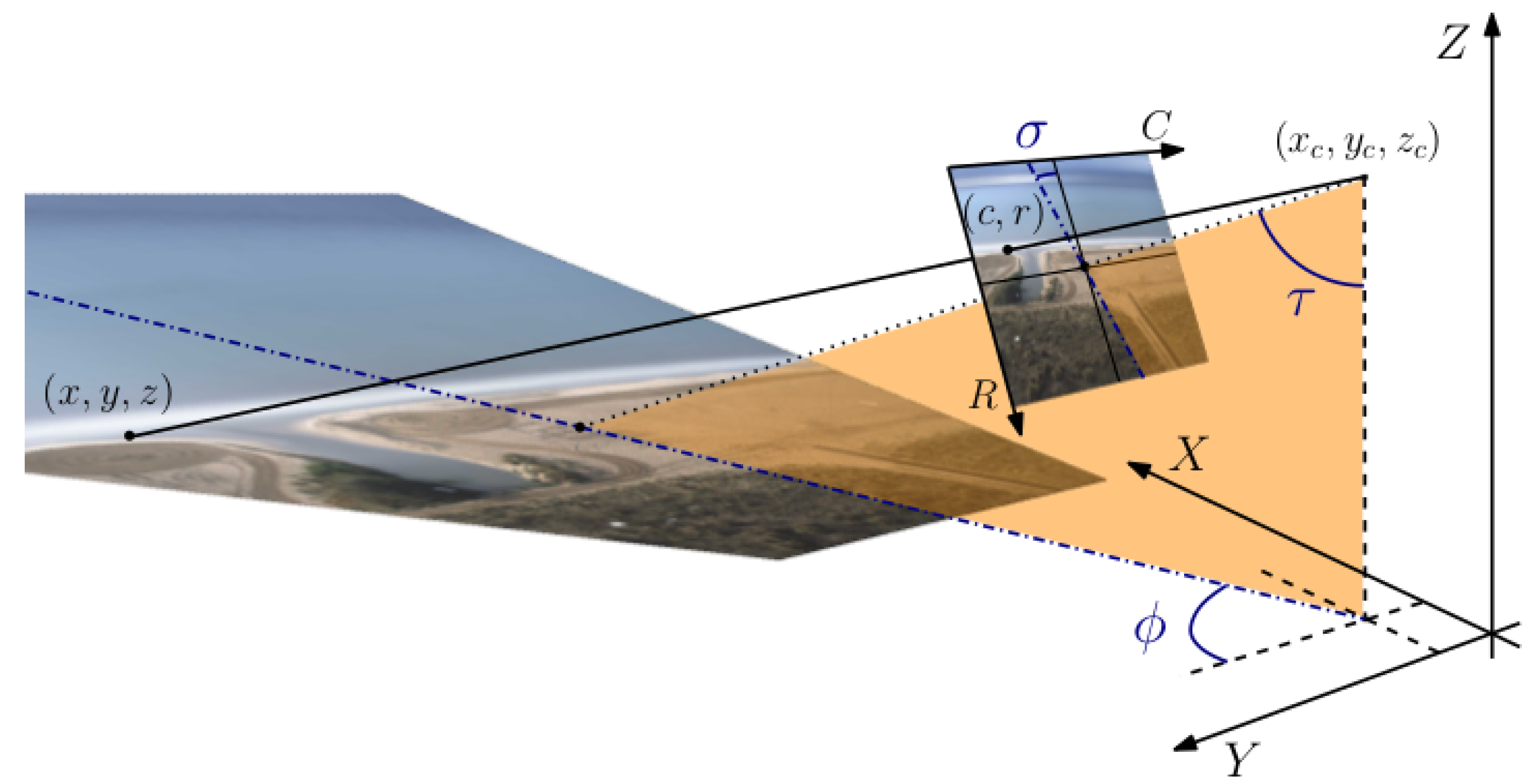
The transformation of images (2D) to real physical space (3D) is usually performed following photogrammetric procedures in which the characteristics of the optics (intrinsic parameters) and the location and orientation of the camera (extrinsic parameters) have to be obtained [25,26]. Intrinsic calibration yields optics parameters of the camera (distortion, pixel size and decentering) and allow elimination of the image distortion induced by the camera lens. Extrinsic calibration allows determining the camera position (, , ) and orientation (, , ), Figure 1, which allows associating each pixel of the undistorted image with real world coordinates (providing, usually, the elevation z).
Extrinsic calibrations are obtained using Ground Control Points (GCPs, pixels whose real-world coordinates are known). The GCPs can also be used for intrinsic calibration, which is often obtained experimentally in laboratory [27,28,29]. Generally, Argus-like video monitoring systems are fully (intrinsic and extrinsic) calibrated at the time of installation, and then extrinsic calibrations are performed at a certain frequency (bianually, e.g., [14]) or when a significant camera movement is noticed.
However, it has already been observed that calibration parameters change throughout the day for a variety of reasons, including thermal and wind effects [30,31], as well as over longer time periods, due to natural factors and/or human disturbance [31,32]. If the calibration of all individual images is not adjusted, the quantitative information obtained could have a significant error, leading to inaccurate quantification in shoreline trends, hydrodynamic data such as longshore currents, wave celerity or runup and, in turn, nearshore bathymetries.
Although the importance of intra-day fluctuations was already reported by Holman and Stanley [7] in 2007, this problem has been disregarded in most studies with coastal video monitoring systems. Recently, Bouvier et al. [31] analyzed, in a station consisting of five cameras, variations in the orientation angles of each of the cameras during one year. From the manual calibration of about 400 images per camera, they identified the primary environmental parameters (solar azimuthal angle and cloudiness) affecting the image displacements and developed an empirical model to successfully correct the camera motions.
This approach has the disadvantage that it does not automatically correct variations over long periods of time, in addition to requiring manual calibration of a large number of images. In order to achieve the highest number of calibrated images while minimizing human intervention, the strategy followed in other studies [30,32,33,34] has been to automatically identify objects and to use their location in calibrated images for their stabilization.
Pearre and Puleo [30] located some features at selected Regions Of Interest (ROI) from a distorted calibrated image into other images to obtain the relative camera displacements between images and then recalculate the orientation of the cameras (tilt and azimuth angles) for each image. Relative shifts of the ROIs were then obtained by finding the correlation peak of correlation matrices. Accurate recognition of pixels corresponding to GCPs in images, using automatic algorithms such as SIFT (Scale-Invariant Feature Transform, [35,36]) or SURF (Speeded-Up Robust Features, [37]), allowed not only to re-orient the cameras but also to compute the extrinsic calibration parameters of each individual image [33,34].
Recently, Rodriguez-Padilla et al. [32] proposed a method to stabilize 5 years of Argus-like station images by identifying fixed elements on images and then correcting the orientation of the cameras by computing deviations with respect a reference image. In this study, CED (Canny Edge Detector, [38]) was used to identify permanent features, such as corners or salients, under variable lighting conditions at given ROIs. In all imaging stabilization studies carried out to date in the coastal zone, they assumed that identifiable features were permanently present, which were used to correct the orientation of cameras or to carry out the complete calibration of the extrinsic parameters. However, in many Argus-like stations, when installed in natural environments, such as beaches or estuaries, the number of fixed features is very limited or non-existent over long periods.
In this paper, we explore image calibration by automatically identifying arbitrary features, i.e., without pre-selection, in the images to be calibrated and in previously calibrated images. Provided that fixed features will be considered very limited, it will not be possible to calibrate the images on the standard GCPs approach, as was done in [24]. Alternatively, we relate pixels of pairs of images through homographies, the main assumption of this work being that the position of the camera position is nearly invariant.
As a counterpoint, there is no need to impose any constraint on either the intrinsic calibration parameters of the camera (lens distortion, pixel size and decentering) or on its rotation. The automatic camera calibration was applied to three video monitoring stations. Two of them operate on beaches of the city of Barcelona (Spain), where there are many fixed and permanent features, and the third one was on the beach of Castelldefels, located southwest of Barcelona, where the number of fixed points is very limited.
The main aim of this paper is to present a methodology, departing from a small set of manually calibrated images, to automatically calibrate images without the need of prescribing reference objects and to evaluate their feasibility. Next, Section 2 presents the basics of mapping pixels corresponding to arbitrary objects between images and the methodology to process points in pairs of images in order to obtain automatically the calibration of an image. Section 3 presents the results that will be discussed in Section 4. Section 5 draws our main conclusions for this work.
2. Methodology
2.1. Camera Equations and Manual Calibration
Given the real world coordinates of a point, , the corresponding (distorted) pixel coordinates, column c and row r (Figure 1), are given by
where stands for the radial distortion, s for the pixel size (the pixel is assumed squared), and are the pixel coordinates of the principal point (considered herein at the center of the image), and u and v are the undistorted coordinates in the image plane
where is the camera position (or “point of view”) and , and are orthonormal vectors defined by the camera orientation, i.e., by the eulerian angles (azimuth), (roll) and (tilt) in Figure 1.
Equation (1) represents a reasonable simplification of more complex distortion models: the radial distortion was assumed parabolic and tangential distortion neglected. This simplified model was shown to be able to model the distortion of common cameras [39] and, in particular, the cameras considered in this work. The eight free parameters of the model are the camera position, , the three eulerian angles (, and ), as well as and s.
2.2. Manual Calibration of a Single Image
Given an image, the eight free parameters of the model can be obtained from a set of N Ground Control Points (GCPs), pixels of the distorted image whose real-world coordinates are known, i.e., N tuples with . The free parameters can be found by minimizing the reprojection error (see, e.g., [40]):
where and are the values obtained from using model Equations (1) and (2) with the proposed parameters. Whenever the horizon line can be detected, it can also be introduced in the optimization process by minimizing , where is the horizon line error: the root mean square of the distances from the pixels detected in the horizon and the horizon line as predicted by the calibration parameters (see, e.g., [41]). Hereafter we will refer to error whether or not the horizon line is detected, assuming that if the horizon line is not available.
2.3. Manual Calibration of a Set of Images
A set of J images, for which GCPs and, in some cases, horizon line pixels are available, is calibrated by minimizing the total error of the set, i.e., . We consider here three different approaches:
- Case 0:
- Different values of and for each image and common values for and s ( unknowns).
- Case 1:
- Different values of and s for each image and common values for and ( unknowns).
- Case 2:
- Different values of and s for each image ( unknowns).
2.4. Homographies
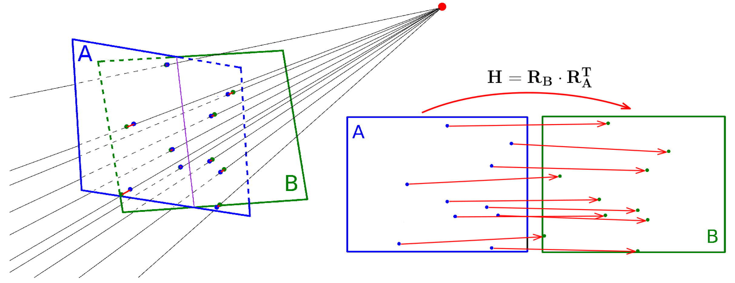
Consider now two images captured at the same point of view (“A” and “B” in Figure 2) but with a different orientation of the camera (case 0) or, even, with different cameras (case 1). The points in the projective planes corresponding to the same ray, i.e., one same point in real space, can then be transformed by an “homography”. The relationship between the undistorted coordinates u and v corresponding to one spatial point as seen in two different images (“A” and “B”, with different angles and intrinsic parameters) is given by [42]:
where corresponds to the i-th row and j-th column of the rotation matrix
The rows of matrices and are the unit vectors , and of images B and A, respectively.
2.5. Automatic Calibration
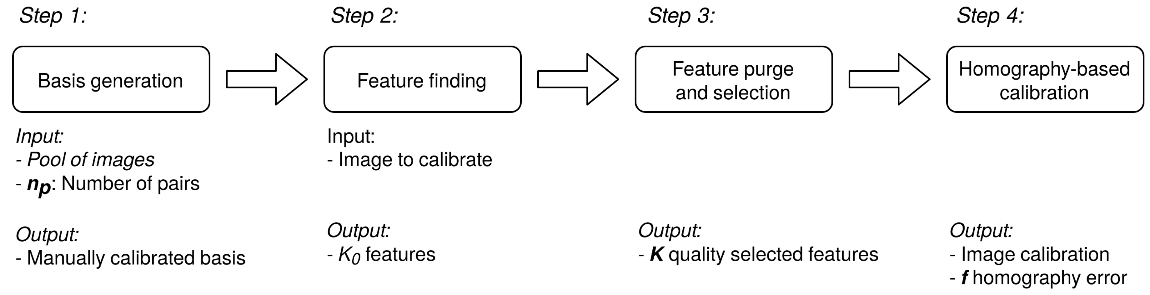
The automatic calibration of an image was performed in four steps that are schematized in Figure 3. First, a set of (manually) calibrated images is generated, which will be referred to as basis (step 1). Next, common features between the image to be calibrated and each of the basis images are identified (step 2). These pairs are then purged to remove erroneous matching features, and, from the remaining set of features, a selection is made (step 3). Finally, this selection is used to calibrate the image (step 4).
The details of each of the steps are described below. For simplicity, the automatic calibration procedure is described for case 0, i.e., when the camera position , and s are the same for all images. The case 1 will be discussed, briefly, afterwards. Table 1 summarizes the parameters resulting from the automatic calibration procedure and that are used to present and discuss the results.
2.5.1. Basis Generation
To calibrate images automatically, a set of manually calibrated images was used. This set of images will be referred to as “basis”. Any set of calibrated images of a camera can be considered as a basis. However, the ideal would be to have the smaller number of basis images to automatically calibrate the largest number of images. Here, we propose a method to generate such a basis, but we emphasize that alternative procedures (including, e.g., cluster analysis or random selection) can be used instead.
The pool of images from which to obtain the basis has, here, images covering different years, seasons and hours within the day. In a first step, using matching algorithm ORB [43], any pair of images of the pool are compared to each other. For each comparison, only the best pairs of features (according to ORB) in each cell of a grid on the image are considered. Then, the basis is made up by adding images to it in order to maximize the number of images of the pool with at least cells having common features with the basis images.
The procedure continues until the number of images of the pool that have cells with pairs with the basis is above . The number of required pairs, , is based on the minimum number of pairs to perform the calibration of an image (i.e., for case 0). As not all features will be useful, a higher number should be taken. Note that, the higher the , the more images will contain the basis.
Once the basis has been established, the manual calibration of this set of images is carried out. The values of the camera position , and s are set. In addition, as the angles of the cameras are known for these images, their rotation matrices , and the homographies between basis images are also known.
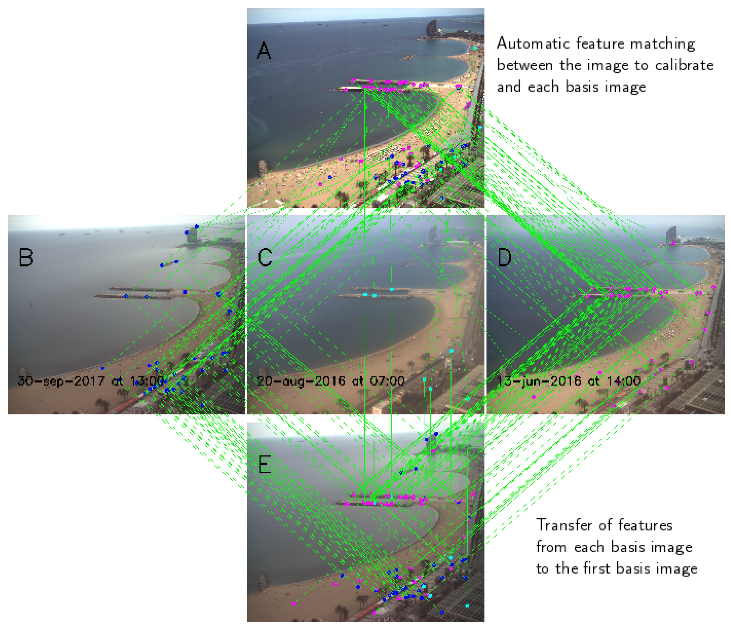
2.5.2. Feature Finding
Given an image to be calibrated and one basis image, the set of pairs of pixels that according to ORB correspond to the same features is found. Using the fact that the basis images are calibrated, the pixels identified in each of the basis images are transferred to a unique basis image, that, in our case, is the first basis image. Hence, a set of pairs of pixels in the image to be calibrated (, ) and the in the first basis image (, ) corresponding to the same features is obtained, with . The number of pairs will be the sum of pairs encountered with each basis image.
Figure 4 illustrates this step up to this point. Next, the values of and s and Equation (1) are used to transform these pixels to undistorted coordinates in the image to calibrate (, ) and in the first basis image (, ). These pairs of undistorted coordinates must be related through an homography (Equation (4)) that involves both the rotation matrix of the image to calibrate , which depends on the unknown angles (, , ), and , which is known.
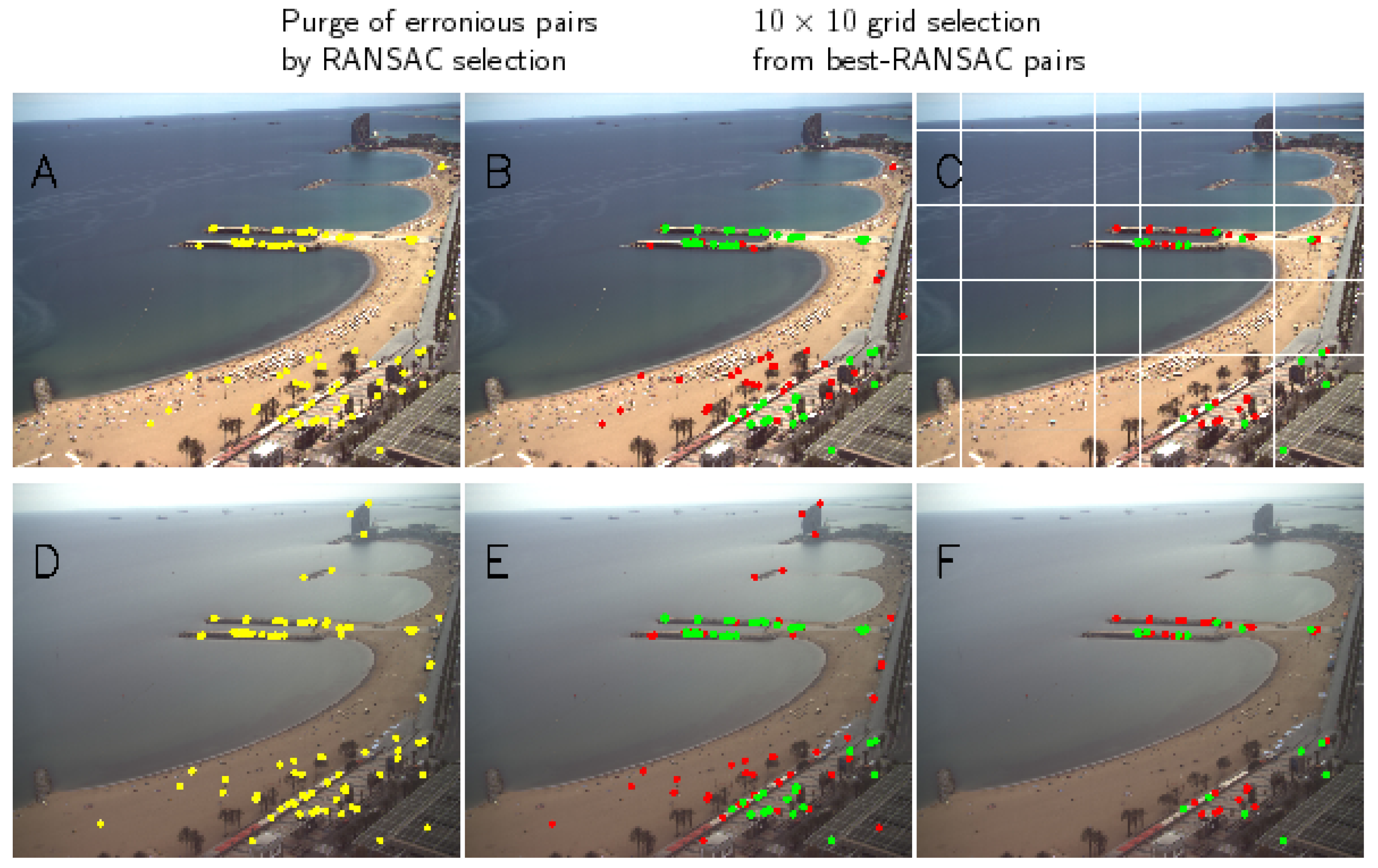
2.5.3. Feature Purge and Selection
Automatic matching algorithms do not always succeed, as can be seen in the images of Figure 5A,D. Therefore, prior to obtaining the three unknown angles, a purge of erroneous pairs of features should be done. A RANSAC (RANdom SAmple Consensus) [44] is performed to the pairs undistorted coordinates using a homography as the model. In this way, a subset of pairs that actually correspond to the homography is obtained (green points in Figure 5B,E; the red dots being disregarded). Further, for the pairs to be more uniformly distributed along the image, out of the remaining pairs, only the best pairs (according to the homography) of each cell of a grid on image to calibrate are considered (green dots in Figure 5C,F). As a result, features were obtained for calibration.
2.5.4. Homography-Based Calibration
From the final subset of K features, we found the rotation matrix , which minimizes a reprojection-like error function, hereafter “homography error”,
where are the undistorted coordinates of the k-th feature in the first image of the basis and is the transformation, through and equation (3), of this feature in the image to calibrate to the first basis image. Recalling Equation (1), the term was introduced in Equation (5) and thus the homography error f is expressed in (undistorted) pixels.
The outputs of the automatic calibration of an image are , and , as well as the minimized f and the number of pairs, K. These last two values, f and K, will be helpful in assessing the quality of the automatic calibration: small homography errors f and large K should correspond to better results.
If case 1 applies, the above algorithm remains the same except that, in order to transform to through Equation (1), unknown values of and s for the image to calibrate are required and have to be obtained recursively. Case 1 corresponds to CoastSnap [15], a citizen science project for beach monitoring.
2.6. Study Sites and Video Monitoring Stations
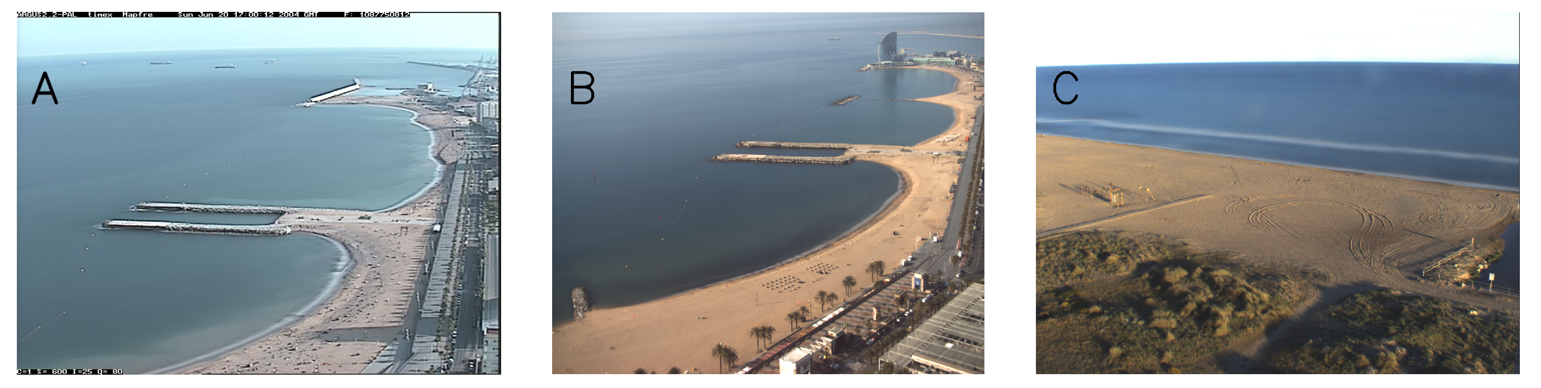
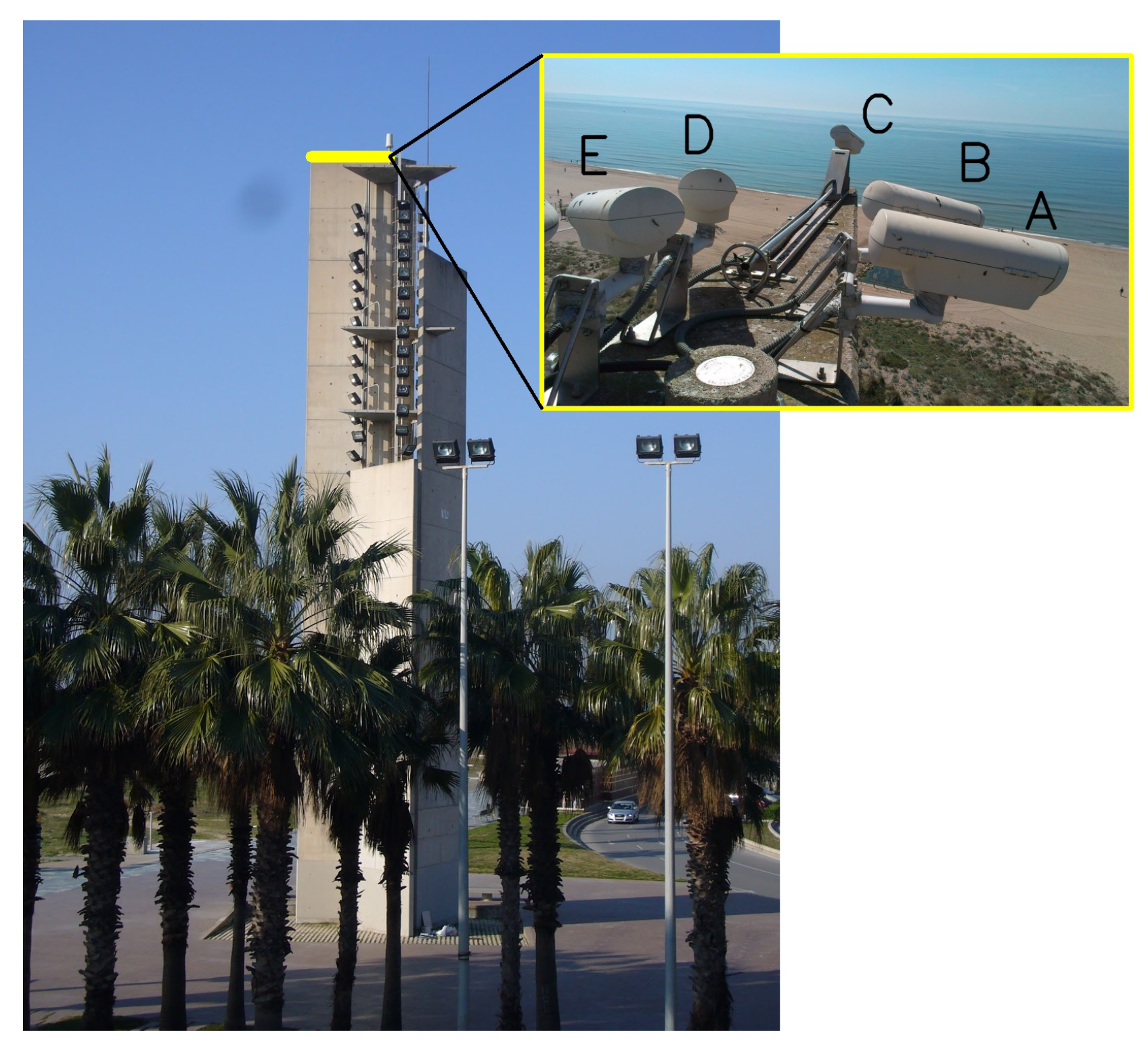
Images of three cameras from different Argus-like stations are considered in this work (Figure 6). Station BCN1 overviewed Barcelona beaches from 2001 to 2015 with a set of five cameras [14] (Figure 6A shows the one considered here, ). This set of cameras was replaced in 2015 by a set of six cameras of higher resolution (herein named station BCN2, Figure 6B, ), which are currently running. A third station, CFA1, with five cameras, is running on Castelldefels beach from 2010 [45] (Figure 6C, ). Note that images from BCN1 and BCN2 include plenty of permanent features (wave breakers, promenades, buildings, …), which are to help in the automatic calibration.
All stations provide, every daylight hour, one snapshot as well as one timex (time average image) and one variance image [7]. The pools of timex images from which to obtain the basis were obtained with a certain time step to ensure images for all day hours. The parameters to obtain the pool of images for each camera are shown in Table 2.
2.7. Code Availability
The source code to calibrate a set of images from a basis of images that are calibrated manually is freely available on GitHub (https://github.com/Ulises-ICM-UPC/UCalib (accessed on 15 July 2021)). The code is accompanied by descriptive documentation and, as an example, the script and the corresponding images. This code performs the calibration of the basis images (step 1) and the calibration of the images (steps 2 to 4).
3. Results
3.1. Basis of Images
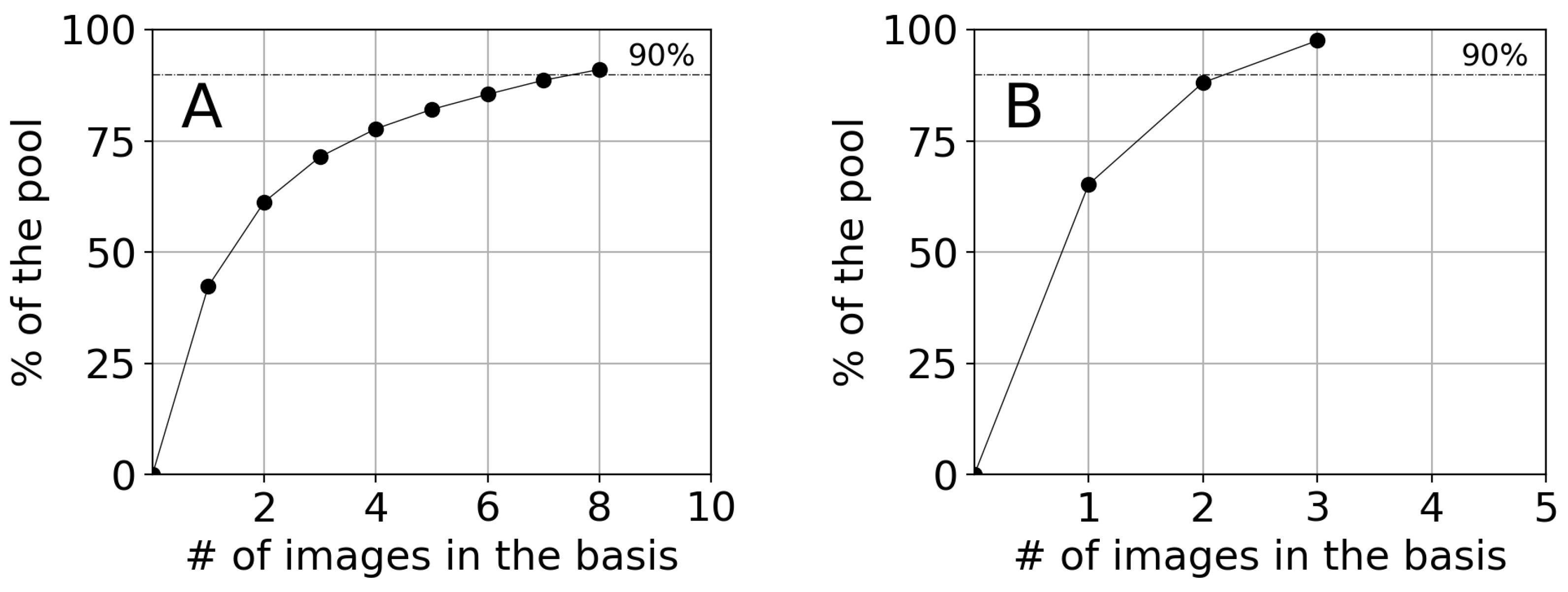
Figure 7 shows, for BCN1 and BCN2, the evolution of the percentage of pool images with (or more) cells having pairs with the basis images as new images are incorporated to it (recall Section 2.5.1). From Figure 7, the basis has eight images for BCN1 and only three for BCN2 (Figure 4B–D). In both cases the basis images are spread over time, covering different years, months and day hours. Further, they include a variety of weather conditions.
The basis of station CFA1 is built up of 20 images chosen randomly out of 40 calibrated images available. In order to have a rough idea of the capability of this basis to calibrate any given image, we computed the number of images of the pool that had four (or more) cells with pairs with the basis. The result was of the 392 pool images. This value, much smaller than , indicates that this basis will likely allow calibrating a smaller percentage of images in practice.
By increasing the number of required cells in the procedure proposed to obtain basis (i.e., being more demanding according to Section 2.5.1), the number of images of the basis images required to reach of the pool images is increased. For example, if , the number of images in the basis is increased to 14 for BCN1 and 4 for BCN2. For , the values are 24 (BCN1) and 5 (BCN2). While trends observed for (images spread over time and weather conditions) still remain, having more images in the basis should allow for the automatic calibration of a larger amount of images. This fact is confirmed in Section 3.3 and Section 3.4 below.
3.2. Manual Calibrations of the Basis Images
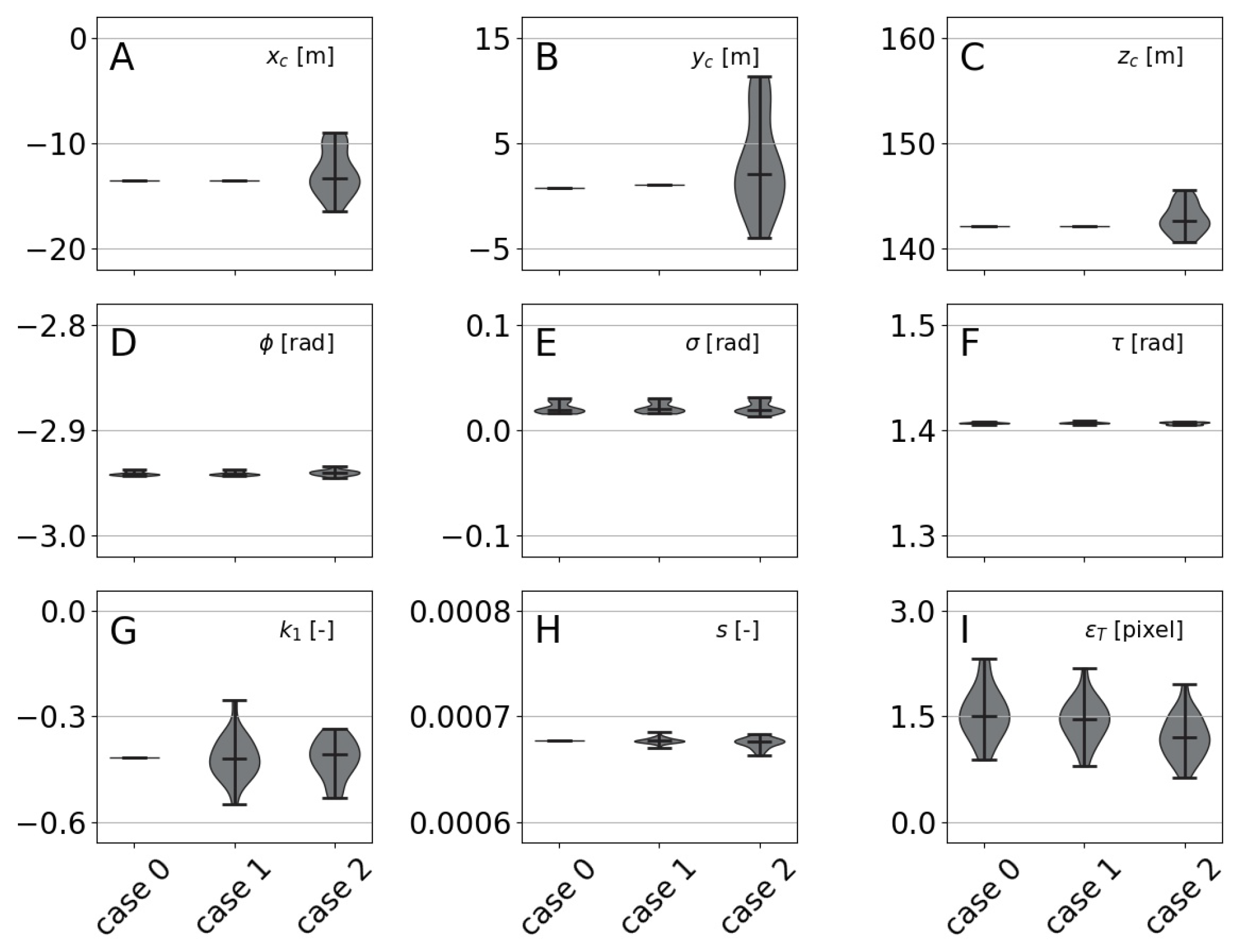
The basis images were calibrated considering the three approaches in Section 2.1 (cases 0, 1 and 2). For illustrative purposes, the results for the largest basis, i.e., BCN1 for (with 24 images), are shown in Figure 8. Similar results were obtained for other stations and basis.
Figure 8 shows the histograms for the eight calibration parameters and calibration error . For cases 0 and 1, the camera position (, and ) collapses in a single value. For case 0, the intrinsic parameters ( and s) also collapse. Collapsed values always fall close to the average value of the corresponding distributions, which is an indication of the results robustness. However, the most relevant issue is that the errors for all three cases are very similar (the same holds for all the basis and stations, Table 3). In conclusion, the above results justify the use, hereafter, of case 0, with constant and the intrinsic parameters and s.
3.3. Critical Values for the Homography Error f and the Number of Pairs K
To analyze the performance of the procedure proposed in Section 2.5 and to understand how the output parameters f and K can be used to assess the quality of the automatic calibration, the procedure was applied to sets of “control” images: images with known GCPs (and, in some cases, horizon points). For BCN1 there were 67 control images (which include the images for all basis).
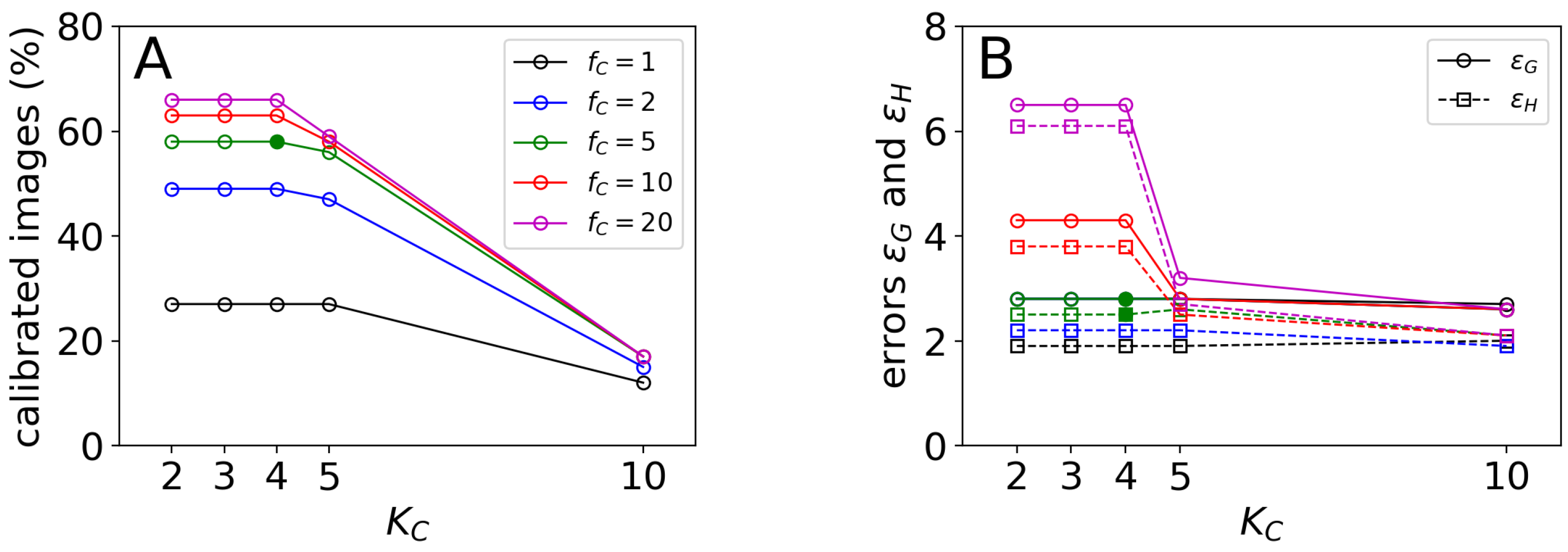
For , for which the basis had eight images, the remaining 59 control images were automatically calibrated: Figure 9 shows the percentage of images calibrated with and for different values of and . The more demanding conditions (smaller allowed and larger required number of pairs ), the smaller the percentage of the 59 images satisfying both conditions (“successful” images). As shown in Figure 9A, for the proposed values, this percentage ranges from , in the most demanding condition, up to in the most relaxed one.
Figure 9B shows the 95th percentile of errors and as computed from the GCPs and horizon points using the corresponding automatic calibration (for the successful calibrations). Interestingly, the 95th percentile of both errors diminished as the conditions became more demanding, i.e., as decreased and increased. In other words, the imposed conditions on f and K were actually a good measure of the expected quality of the automatic calibration. According to Figure 9 and to equivalent results for other stations (using 46 control images for BCN2 and 20 for CFA1) and values of (not shown),
appear to be a good compromise between the percentage of calibratable images and the quality of these automatic calibrations. Table 4 shows the values of percentages and the 95th percentile of errors and of the successful control images for and and for the different stations. From Table 4, the higher , i.e., the more basis images, the more control images were successfully calibrated.
3.4. Automatic Calibration of Several Years
Several years of images were automatically calibrated for all three stations (see Table 5). Using the critical values proposed above ( and ), Table 6 shows the percentage of automatically calibrated images satisfying and . While the values are different than in Table 4, the same trends are observed, namely: (1) the percentage increased with and (2) the worst station was CFA1, and the best one was BCN2. Table 6 also shows the results for more restrictive values (, ): the percentages are smaller for these more restrictive conditions, particularly for BCN1 and CFA1.
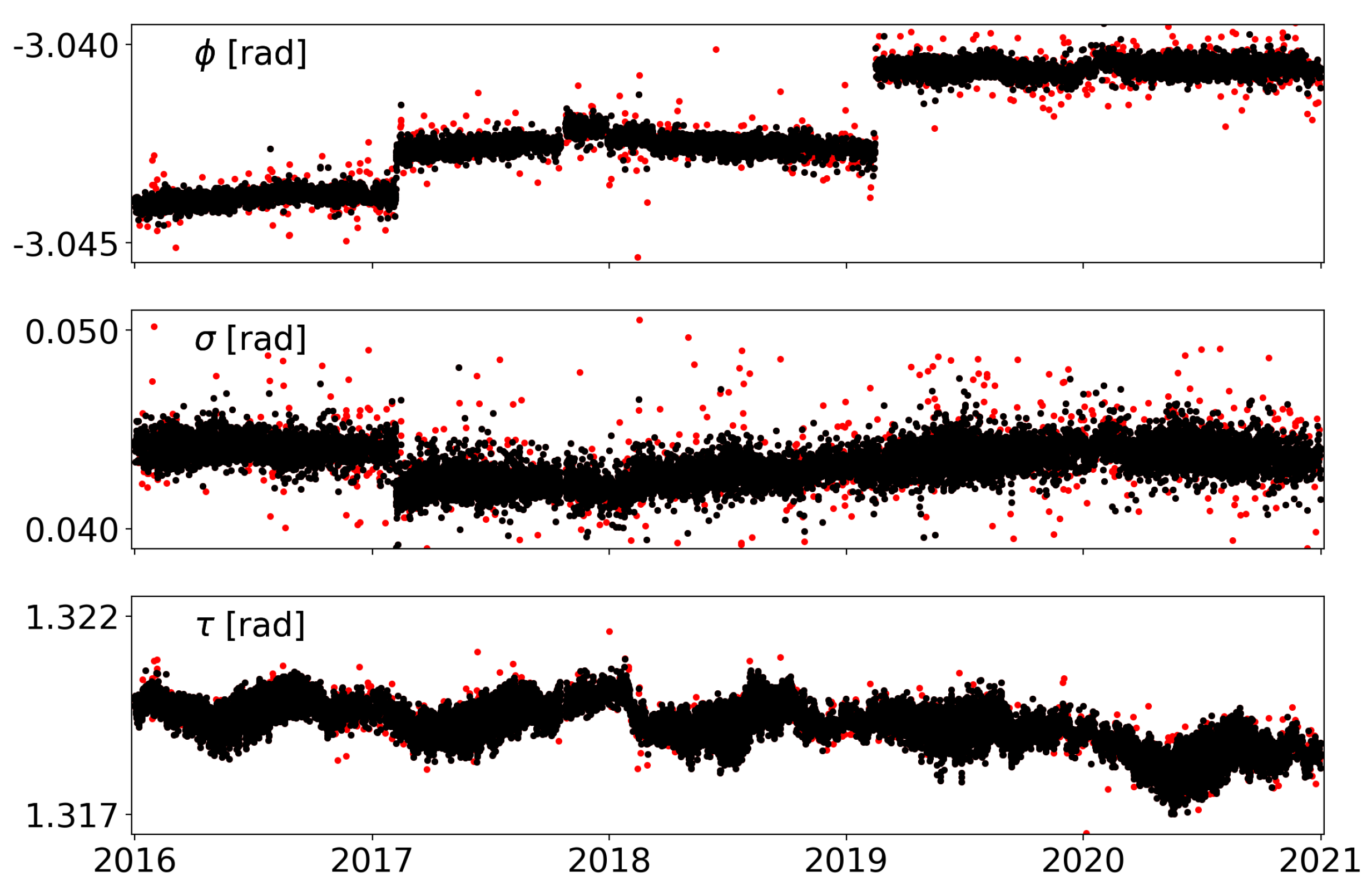
For illustration purposes, Figure 10 shows the time evolution of the eulerian angles for BCN2 and for and ( of the total images according to Table 6). In this Figure, the black dots also satisfy more demanding conditions and ( according to Table 6). Most of the outliers in Figure 10, mainly observable in roll , correspond to red dots, i.e., those not satisfying the more demanding conditions.
The signal also shows a noise that is related to intra-day oscillations (see below). This noise has, in tilt , a seasonal behavior, with larger amplitudes in summer than in winter. Several permanent jumps are also observed in azimuth , the most significant at the beginning of year 2019. These jumps correspond to uncontrolled movements of the camera (e.g., due to a gust of wind) and are not always easily detected by visual inspection of the images.
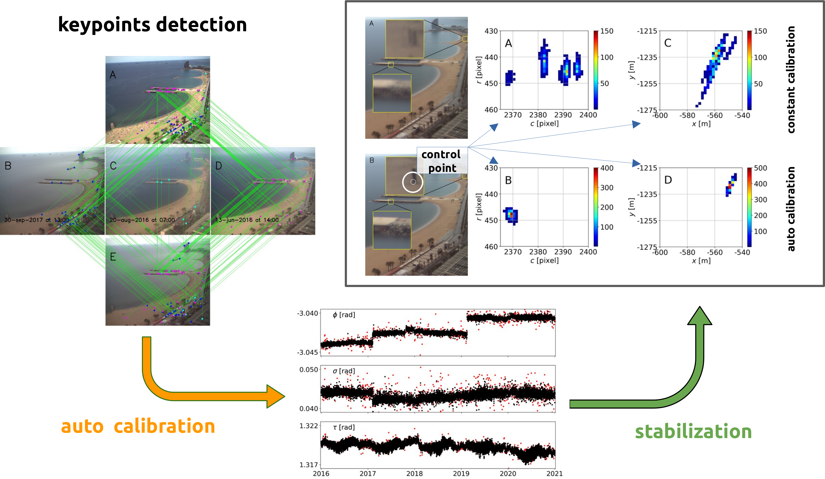
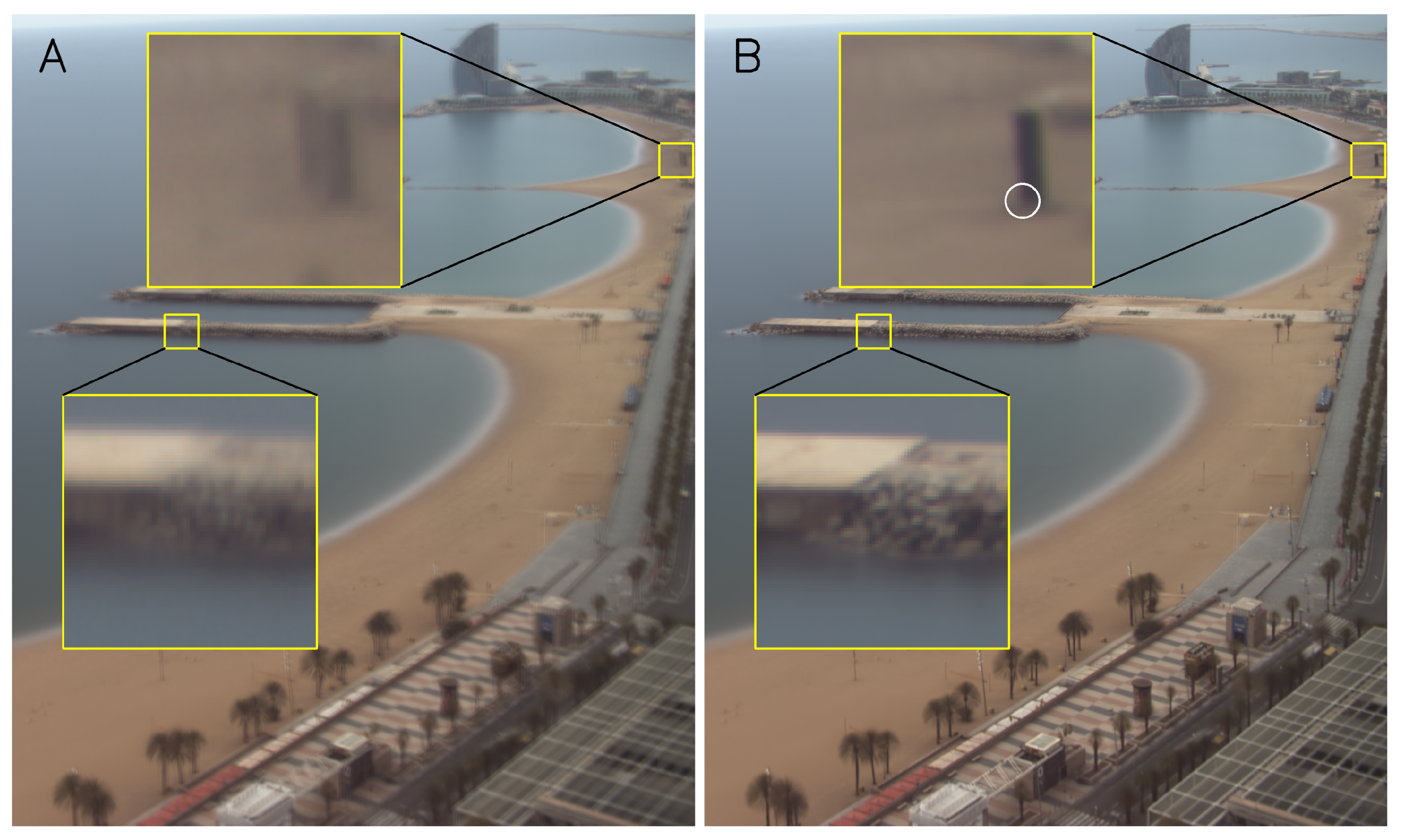
Following similar procedures to those in Section 2, which allow transforming pixels coordinates from two calibrated images, all images can be represented as in, e.g., the first image of the series, i.e., images are stabilized or registered. Time averaging the resulting images and comparing the result with the time average of raw images is a usual way to verify that the stabilization (here automatic calibration) is being performed well (e.g., [32]). Figure 11 shows the results for the same conditions as for Figure 10 (, and ). The blurring observed in Figure 11A is very much reduced in Figure 11B (stabilized).
While obtaining the timex of stabilized images is a common way to show that automatic calibration is working properly, it does not allow for a quantification of the errors before and after the process. To illustrate such a quantitative information, one same feature was manually tracked in the images through the series of years (a total of 2000 positions, randomly distributed in time along the years, were obtained). The feature is the left bottom corner of the sculpture marked with a white circle in Figure 11B. The estimated error when manually tracking the feature was around .
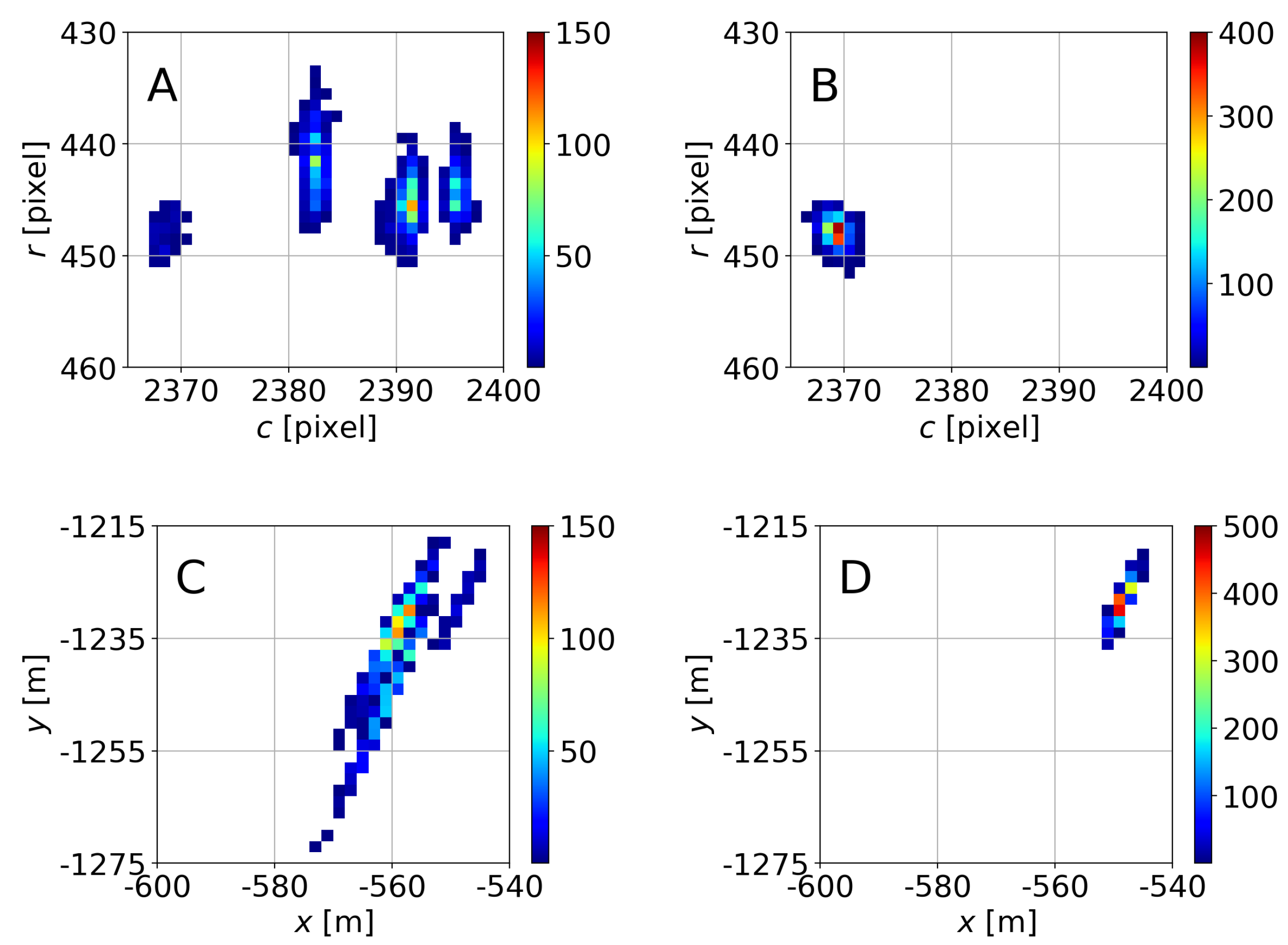
Figure 12A shows the distribution of the pixels coordinates: four clouds were observed, corresponding to the permanent jumps in Figure 10. The Root Mean Square (RMS) of the distances of pixels to the center of mass of the distribution was , and the elongated shape of the clouds in this Figure 12A was due to intra-day oscillations. When all pixel coordinates were stabilized to the first image using automatic calibrations, the result (Figure 12B) was a single compact cloud. The RMS of the distances to the center of mass of the distribution was reduced to , consistent with the estimation of the error when tracking the feature.
These results can be, alternatively, expressed in meters (Figure 12C,D). For this purpose, we considered that the feature was at . If all clicked pixel coordinates (Figure 12A) are projected into the -plane using a constant calibration (the first one, here), the resulting distribution is shown in Figure 12C. However, if the corresponding automatic calibrations are used for each pixel, the distribution is the one in Figure 12D, whose RMS of the distances to the center of mass is .
This RMS, noise, is due, in part, to the manual tracking procedure but also to the possible errors in automatic calibrations. Reasonably assuming that the center of mass of the distribution in Figure 12D, at , corresponds to the actual position of the point, the RMS of the distances in Figure 12C to this position is , with a maximum distance between points of the cloud being around . These errors are directly those that would be transmitted to the position of the shoreline if, e.g., the objective was to calculate the area of a beach.
4. Discussion
4.1. Camera Position and Intrinsic Calibration
The proposed process for georeferencing images using homographies is based on the assumption that cameras remain nearly immobile. This hypothesis may appear to be contradicted by the results of this study since the full manual calibration (case 2) of basis images shows a movement of the cameras of several meters in the three spatial directions. These movements must be taken with caution, as displacements of up to 20 m meter in the horizontal and almost 10 m in the vertical are absolutely unrealistic. The manual calibration of several images forcing a common camera position (case 1) provided a camera position that corresponded approximately to the average position obtained in case 2.
Calibration errors resulting from these two cases are so that the difference of the mean values of the errors are less than half of the statistical deviations of the errors (see Table 3). We understand that, in the full calibration, the apparent movement of the cameras was actually compensated by other parameters of the calibration (see Figure 8), mainly through the intrinsic parameters (radial distortion and pixel size). Calibrations forcing common values of the intrinsic parameters (case 0) have errors that are again equivalent to those of the other two cases.
We conclude, therefore, that the apparent camera movements and their internal deformations can be perfectly assimilated by the changes in camera orientation. Furthermore, since the complete calibration of the camera results in unrealistic displacements, we consider that it is more appropriate to allow only changes in the camera orientation and thus avoid spurious fluctuations in the position and intrinsic parameters. The results for the three calibration approximations also validate approaches made in previous studies (e.g., [31,32]) in which the camera positions were fixed without further verification.
4.2. Method Applicability
The results show that the method described here can be used to calibrate automatically images from Argus-type stations from a basis of manually calibrated images. In contrast to other studies (e.g., [32]), it was not necessary to predefine targets in certain regions of interest. Instead, it is feasible to use arbitrary features located in the real world with unknown exact locations. This makes the method very flexible as it does not require permanent points in the image. The only important conditions are that features must be automatically detected and that the cameras must remain motionless.
The results demonstrated that cameras of different resolutions did not cause any major inconvenience. Neither does the fact that the environment is urban or natural and, therefore, with a large number of ephemeral elements. However, a number of images could not be calibrated due to the lack of common features with basis images. It is possible that the use of other algorithms (e.g., a Canny Edge Detector, [38]) could improve the performance. This remains for further research.
As an extension of the present work, the same method could be used in stations where several cameras are used to take images from a fixed position, as it is the case of the CoastSnap stations [15]. In this case the calibrations share a unique location; however, both the images from the basis and the images to be calibrated would have different internal calibrations. In this scenario, the calibrations discussed in Section 2.1 and Section 2.5 for the specific case 1 would need to be applied. The analysis of the method presented here on CoastSnap type stations is beyond the scope of this paper.
There is also an option to perform calibrations based on homographies when the camera position is not fixed (case 2) as occurs for cameras mounted on UAVs. This option has not been further developed in the paper as it is a very theoretical approach. In the case where the camera moves, the homography between different images is only valid when the points in the real world are placed over a common plane. For some beaches, it can be assumed that the surface is at the same height, as [24] does in a first estimation; however, in general, this approximation can introduce significant errors.
4.3. Horizon Line in Manual Calibrations
Whenever the water zone is of interest [e.g., for bathymetry inversion [21,24]], it is necessary that calibrations perform well at it. Whenever the horizon line is observable, errors at the horizon give a hint of the performance of the calibration in the water zone, far from the GCPs for calibration, and also far from the features detected by the ORB algorithm (green dots in Figure 5C,F) for automatic calibration. Table 4 (errors using control images) shows the 95th percentile of the errors at the GCPs, , as well as on the horizon, . The results of Table 4 list the manual calibrations of the basis where the horizon line was introduced in the optimization procedure whenever it was available. As seen, the errors in the horizon, , are of the same order of the errors .
However, it is very often the case that the horizon is not considered in the manual calibrations. If the basis images are manually calibrated ignoring the error in the horizon, the errors of the derived automatic calibrations are shown in parentheses in Table 4. Considering the horizon in the calibration of basis images has little effect on but significantly reduces the errors . This is despite that the automatic calibration uses the same ORB points in both cases. In other words, the better performance of the manual calibrations of the basis in regard the horizon (and, likely, in the water zone) is transmitted to the automatic calibrations.
4.4. Critical Values for the Homography Error and the Number of Pairs
When performing the automatic calibration of an image, the output consists of the calibration parameters together with f (pixels) and K. Based on the results on control images, we decided that an automatic calibration can be considered to be good if and , with critical values of and . These values were chosen as a compromise between the percentage of calibratable images and the quality of the calibrations for all three stations and different basis. For the stations under consideration, these critical values appear to be essentially independent of the station and basis. However, the values of and can be arbitrarily chosen by the user. Low and high , i.e., more restrictive conditions, will reduce the percentage of automatic calibrations, which should be more trustful.
Figure 10 shows the results for and (black dots), showing that most of the outliers are avoided. In order to reduce the outliers in Figure 10 for and (all dots, red and black), one could alternatively try time filtering taking into account that the characteristic filtering time window has to be small enough not to filter the intra-day oscillations of the signal. In addition, from the results for all three stations, the more relevant questions to obtain a large percentage of good automatic calibrations appear to be: (1) the amount of fixed features observable in the images (BCN1 and BCN2 give better results than CFA1) and, less, (2) the image size (BCN2 works better than BCN1).
4.5. On the Origin of the Camera Movements
One main result from the manual calibration of the basis is, as mentioned, that the camera position can be considered constant in time (Figure 8 and Table 3) and that all the modifications of the camera can be assumed by the three eulerian angles. This does not necessarily mean that the camera is not having any movement, but that these movements can be considered sufficiently small and can be compensated by the eulerian angles.
According to [31], “the viewing angle deformations are controlled by thermal deformation of the pole where they are mounted”, and they proposed predictive expressions to correct the viewing (eulerian) angles based on the cloudiness, solar azimuth angle, …. In this work, similar to [32], the goal was not to propose such an expression for our stations but to automatically calibrate as many images as possible departing from a basis of calibrated images.
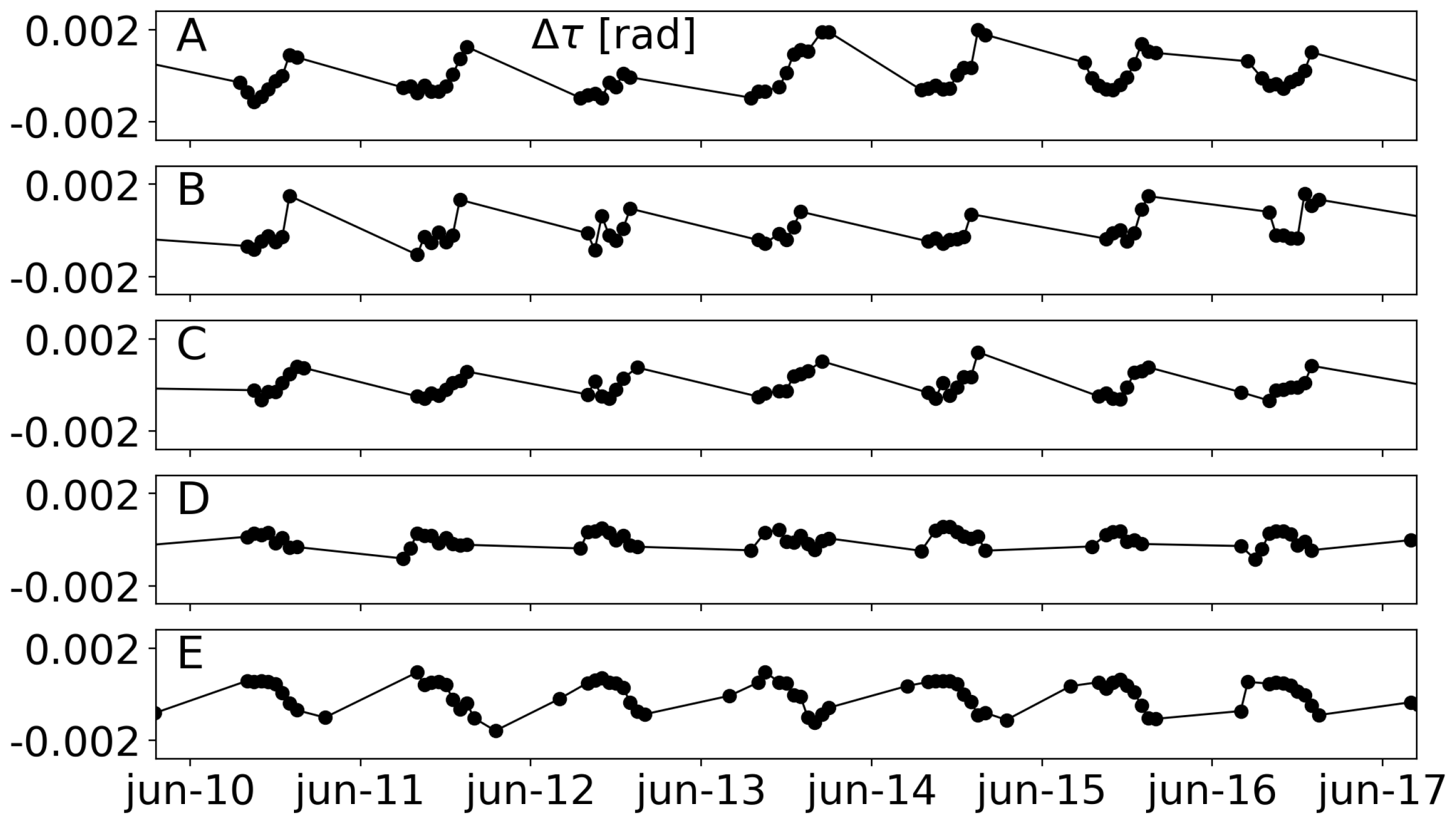
However, once the images have been (automatically) calibrated, it can be of use to shed some light on the possible mechanisms that cause the viewing angles to change. Pretending only to be illustrative, we consider the time evolution of (tilt) for the five cameras in station CFA1 (Figure 13); thus far, only the results for camera D in Figure 13 were shown for CFA1. Figure 14 shows the time evolution of the demeaned angle, , for the five cameras of CFA1 during 7 days in summer 2013. From the figure, the tilt behavior changed from camera to camera. Focusing on the outer cameras (A and E in Figure 13), e.g., while, for camera A, the tilt tended to increase during the daylight hours, the trend was the opposite for camera E, suggesting that the whole concrete structure had a (small) deflection that was captured by the cameras.
5. Conclusions
In this paper, an automatic calibration procedure was proposed to stabilize images from video monitoring stations. The proposed methodology was based on well-known feature detecting and matching algorithms and allows for massive automatic calibrations of an Argus camera provided a set, or basis, of calibrated images. From a theoretical point of view regarding computer vision, the single hypothesis supporting the approach is that the camera position can be regarded to be nearly constant. In the cases considered here (Argus-like station), we proved that the intrinsic parameters and the camera position can actually be considered constant (case 0). However, the procedure proposed here was able to manage the case in which intrinsic calibration parameters change in time, which makes the approach valid for CoastSnap stations.
The number of images of the basis can be chosen arbitrarily (here, through the required pairs, ) and, the higher this is, the more images can be properly calibrated. All the automatic calibrations are performed directly through the basis of images, i.e., second or higher order generations of automatic calibrations have not been considered to avoid error accumulations. If the calibrations are to be applied to analyze the water zone (e.g., for bathymetric inversion), we recommend that the horizon line is introduced as an input in the basis calibration.
The proposed methodology offers the automatic calibration of an image together with the homography error f and the number of pairs K that give a measure of the reliability of the calibration itself. Imposing and , the percentage of calibrated images ranges from for the worst conditioned case (Castelldefels beach, with very few features) to (high resolution cameras in Barcelona, where there are plenty of fixed features), the errors in pixels being significantly reduced (e.g., from to in the analyzed case).
Author Contributions
The first two authors equally contributed to the work. Conceptualization, G.S., D.C. and P.S.; methodology, G.S., D.C. and P.S.; software, G.S., D.C. and P.S.; validation, G.S., D.C. and P.S.; formal analysis, G.S. and D.C.; investigation, G.S., D.C. and P.S.; resources, G.S. and D.C.; writing–original draft preparation, G.S. and D.C.; writing–review and editing, G.S., D.C. and P.S.; visualization, G.S. and D.C.; supervision, G.S. and D.C.; project administration, G.S. and D.C.; funding acquisition, G.S. and D.C. All authors have read and agreed to the published version of the manuscript.
Funding
This research was funded by the Spanish Government (MINECO/MICINN/FEDER) grant numbers RTI2018-093941-B-C32 and RTI2018-093941-B-C33.
Institutional Review Board Statement
Not Applicable.
Informed Consent Statement
Not Applicable.
Data Availability Statement
Not Applicable.
Acknowledgments
The authors acknowledge the useful suggestions from F. Moreno-Noguer and N. Ugrinovic.
Conflicts of Interest
The authors declare no conflict of interest.
Abbreviations
The following abbreviations are used in this manuscript:
| CED | Canny Edge Detector |
| GCP | Ground Control Point |
| ORB | Oriented FAST and Rotated BRIEF |
| RANSAC | RANdom SAmple Consensus |
| RMS | Root Mean Square |
| ROI | Region Of Interest |
| SIFT | Scale-Invariant Feature Transform |
| SURF | Speeded-Up Robust Features |
References
- Smit, M.; Aarninkhof, S.; Wijnberg, K.M.; González, M.; Kingston, K.; Southgate, H.; Ruessink, B.; Holman, R.; Siegle, E.; Davidson, M. The role of video imagery in predicting daily to monthly coastal evolution. Coast. Eng. 2007, 54, 539–553. [Google Scholar] [CrossRef]
- Klemas, V.V. The role of remote sensing in predicting and determining coastal storm impacts. J. Coast. Res. 2009, 25, 1264–1275. [Google Scholar] [CrossRef] [Green Version]
- Santos, C.; Andriolo, U.; Ferreira, J. Shoreline response to a sandy nourishment in a wave-dominated coast using video monitoring. Water 2020, 12, 1632. [Google Scholar] [CrossRef]
- Harley, M.D.; Andriolo, U.; Armaroli, C.; Ciavola, P. Shoreline rotation and response to nourishment of a gravel embayed beach using a low-cost video monitoring technique: San Michele-Sassi Neri, Central Italy. J. Coast. Conserv. 2014, 18, 551–565. [Google Scholar] [CrossRef]
- Guillén, J.; García-Olivares, A.; Ojeda, E.; Osorio, A.; Chic, O.; González, R. Long-term quantification of beach users using video monitoring. J. Coast. Res. 2008, 24, 1612–1619. [Google Scholar] [CrossRef]
- Davidson, M.; Aarninkhof, S.; Van Koningsveld, M.; Holman, R. Developing coastal video monitoring systems in support of coastal zone management. J. Coast. Res. 2006, 25, 49–56. [Google Scholar]
- Holman, R.; Stanley, J. The history and technical capabilities of Argus. Coast. Eng. 2007, 54, 477–491. [Google Scholar] [CrossRef]
- Nieto, M.; Garau, B.; Balle, S.; Simarro, G.; Zarruk, G.; Ortiz, A.; Tintoré, J.; Ellacuría, Á.; Gómez-Pujol, L.; Orfila, A. An open source, low cost video-based coastal monitoring system. Earth Surf. Process. Landf. 2010, 35, 1712–1719. [Google Scholar] [CrossRef]
- Taborda, R.; Silva, A. COSMOS: A lightweight coastal video monitoring system. Comput. Geosci. 2012, 49, 248–255. [Google Scholar] [CrossRef]
- Lippmann, T.C.; Holman, R.A. Quantification of sand bar morphology: A video technique based on wave dissipation. J. Geophys. Res. 1989, 94, 995. [Google Scholar] [CrossRef]
- Wilson, G.W.; Özkan-Haller, H.T.; Holman, R.A.; Haller, M.C.; Honegger, D.A.; Chickadel, C.C. Surf zone bathymetry and circulation predictions via data assimilation of remote sensing observations. J. Geophys. Res. Ocean. 2014, 119, 1993–2016. [Google Scholar] [CrossRef] [Green Version]
- Ribas, F.; Kroon, A. Characteristics and dynamics of surfzone transverse finger bars. J. Geophys. Res. 2007, 112, F03028. [Google Scholar] [CrossRef] [Green Version]
- Coco, G.; Payne, G.; Bryan, K.; Rickard, D.; Ramsay, D.; Dolphin, T. The use of imaging systems to monitor shoreline dynamics. In Proceedings of the 1st International Conference on Coastal Zone Management and Engineering in the Middle East, Dubai, United Arab Emirates, 27–29 November 2005; pp. 1–7. [Google Scholar]
- Ojeda, E.; Guillén, J. Shoreline dynamics and beach rotation of artificial embayed beaches. Mar. Geol. 2008, 253, 51–62. [Google Scholar] [CrossRef]
- Harley, M.; Kinsela, M.; Sánchez-García, E.; Vos, K. Shoreline change mapping using crowd-sourced smartphone images. Coast. Eng. 2019, 150, 175–189. [Google Scholar] [CrossRef]
- Aagaard, T.; Kroon, A.; Andersen, S.; Møller Sørensen, R.; Quartel, S.; Vinther, N. Intertidal beach change during storm conditions; Egmond, The Netherlands. Mar. Geol. 2005, 218, 65–80. [Google Scholar] [CrossRef]
- Aarninkhof, S.; Turner, I.; Dronkers, T.; Caljouw, M.; Nipius, L. A video-based technique for mapping intertidal beach bathymetry. Coast. Eng. 2003, 49, 275–289. [Google Scholar] [CrossRef]
- Soloy, A.; Turki, I.; Lecoq, N.; Gutiérrez Barceló, A.; Costa, S.; Laignel, B.; Bazin, B.; Soufflet, Y.; Le Louargant, L.; Maquaire, O. A fully automated method for monitoring the intertidal topography using Video Monitoring Systems. Coast. Eng. 2021, 167. [Google Scholar] [CrossRef]
- Stockdon, H.F.; Holman, R.A. Estimation of wave phase speed and nearshore bathymetry from video imagery. J. Geophys. Res. Ocean. 2000, 105, 22015–22033. [Google Scholar] [CrossRef]
- Plant, N.G.; Holland, K.T.; Haller, M.C. Ocean wavenumber estimation from wave-resolving time series imagery. IEEE Trans. Geosci. Remote Sens. 2008, 46, 2644–2658. [Google Scholar] [CrossRef]
- Holman, R.; Plant, N.; Holland, T. CBathy: A robust algorithm for estimating nearshore bathymetry. J. Geophys. Res. Ocean. 2013, 118, 2595–2609. [Google Scholar] [CrossRef]
- Simarro, G.; Calvete, D.; Luque, P.; Orfila, A.; Ribas, F. UBathy: A new approach for bathymetric inversion from video imagery. Remote Sens. 2019, 11, 2722. [Google Scholar] [CrossRef] [Green Version]
- Bergsma, E.W.; Almar, R.; Melo de Almeida, L.P.; Sall, M. On the operational use of UAVs for video-derived bathymetry. Coast. Eng. 2019, 152, 103527. [Google Scholar] [CrossRef]
- Simarro, G.; Calvete, D.; Plomaritis, T.; Moreno-Noguer, F.; Giannoukakou-Leontsini, I.; Montes, J.; Durán, R. The influence of camera calibration on nearshore bathymetry estimation from UAV videos. Remote Sens. 2021, 13, 150. [Google Scholar] [CrossRef]
- Holland, K.; Holman, R.; Lippmann, T.; Stanley, J.; Plant, N. Practical use of video imagery in nearshore oceanographic field studies. IEEE J. Ocean. Eng. 1997, 22, 81–91. [Google Scholar] [CrossRef]
- CIRN. CIRN Platform in GitHub. 2016. Available online: https://github.com/Coastal-Imaging-Research-Network (accessed on 15 July 2021).
- Bouguet, J.Y. Visual Methods for Three-Dimensional Modeling. Ph.D. Thesis, California Institute of Technology, Pasadena, CA, USA, 1999. [Google Scholar]
- Sánchez-García, E.; Balaguer-Beser, A.; Pardo-Pascual, J. C-Pro: A coastal projector monitoring system using terrestrial photogrammetry with a geometric horizon constraint. ISPRS J. Photogramm. Remote Sens. 2017, 128, 255–273. [Google Scholar] [CrossRef] [Green Version]
- Andriolo, U.; Sánchez-García, E.; Taborda, R. Operational use of surfcam online streaming images for coastal morphodynamic studies. Remote Sens. 2019, 11, 78. [Google Scholar] [CrossRef] [Green Version]
- Pearre, N.S.; Puleo, J.A. Quantifying seasonal shoreline variability at Rehoboth Beach, Delaware, using automated imaging techniques. J. Coast. Res. 2009, 10, 900–914. [Google Scholar] [CrossRef]
- Bouvier, C.; Balouin, Y.; Castelle, B.; Holman, R. Modelling camera viewing angle deviation to improve nearshore video monitoring. Coast. Eng. 2019, 147, 99–106. [Google Scholar] [CrossRef]
- Rodriguez-Padilla, I.; Castelle, B.; Marieu, V.; Morichon, D. A simple and efficient image stabilization method for coastal monitoring video systems. Remote Sens. 2020, 12, 70. [Google Scholar] [CrossRef] [Green Version]
- Vousdoukas, M.I.; Pennucci, G.; Holman, R.A.; Conley, D.C. A semi automatic technique for Rapid Environmental Assessment in the coastal zone using Small Unmanned Aerial Vehicles (SUAV). J. Coast. Res. 2011, 64, 1755–1759. [Google Scholar]
- Vousdoukas, M.I.; Ferreira, P.M.; Almeida, L.P.; Dodet, G.; Psaros, F.; Andriolo, U.; Taborda, R.; Silva, A.N.; Ruano, A.; Ferreira, Ó.M. Performance of intertidal topography video monitoring of a meso-tidal reflective beach in South Portugal. Ocean Dyn. 2011, 61, 1521–1540. [Google Scholar] [CrossRef]
- Lowe, D.G. Object recognition from local scale-invariant features. ICCV 1999, 99, 1150–1157. [Google Scholar]
- Lowe, D.G. Distinctive image features from scale-invariant keypoints. Int. J. Comput. Vis. 2004, 60, 91–110. [Google Scholar] [CrossRef]
- Bay, H.; Ess, A.; Tuytelaars, T.; Van Gool, L. Speeded-Up Robust Features (SURF). Comput. Vis. Image Underst. 2008, 110, 346–359. [Google Scholar] [CrossRef]
- Canny, J. A Computational Approach to Edge Detection. IEEE Trans. Pattern Anal. Mach. Intell. 1986, PAMI-8, 679–698. [Google Scholar] [CrossRef]
- Simarro, G.; Calvete, D.; Souto, P.; Guillén, J. Camera calibration for coastal monitoring using available snapshot images. Remote Sens. 2020, 12, 840. [Google Scholar] [CrossRef]
- Weng, J.; Coher, P.; Herniou, M. Camera Calibration with Distortion Models and Accuracy Evaluation. IEEE Trans. Pattern Anal. Mach. Intell. 1992, 14, 965–980. [Google Scholar] [CrossRef] [Green Version]
- Simarro, G.; Ribas, F.; Álvarez, A.; Guillén, J.; Chic, O.; Orfila, A. ULISES: An open source code for extrinsic calibrations and planview generations in coastal video monitoring systems. J. Coast. Res. 2017, 33, 1217–1227. [Google Scholar] [CrossRef]
- Hartley, R.; Zisserman, A. Multiple View Geometry in Computer Vision; Cambridge University Press: Cambridge, UK, 2004; p. 670. [Google Scholar]
- Rublee, E.; Rabaud, V.; Konolige, K.; Bradski, G. ORB: An efficient alternative to SIFT or SURF. In Proceedings of the 2011 International Conference on Computer Vision, Barcelona, Spain, 6–13 November 2011; pp. 2564–2571. [Google Scholar] [CrossRef]
- Fischler, M.; Bolles, R. Random sample consensus: A Paradigm for Model Fitting with Applications to Image Analysis and Automated Cartography. Commun. ACM 1981, 24, 381–395. [Google Scholar] [CrossRef]
- Simarro, G.; Bryan, K.R.; Guedes, R.M.; Sancho, A.; Guillen, J.; Coco, G. On the use of variance images for runup and shoreline detection. Coast. Eng. 2015, 99, 136–147. [Google Scholar] [CrossRef]
Figure 1.
Real-world (x, y, z) to pixel (c, r) transformation: camera position (, , ) and eulerian angles (, and ).
Figure 1.
Real-world (x, y, z) to pixel (c, r) transformation: camera position (, , ) and eulerian angles (, and ).

Figure 2.
Homography between the undistorted coordinates in two different images “A” and “B”.

Figure 3.
Diagram of the automatic calibration procedure.

Figure 4.
Illustration of the step 2. Image to calibrate (A), basis of images (B–D) and the first image of the basis, including all the pairs found (E).
Figure 4.
Illustration of the step 2. Image to calibrate (A), basis of images (B–D) and the first image of the basis, including all the pairs found (E).

Figure 5.
Illustration of the step 3. Pixels in the image to calibrate (A–C) and in the first image of the basis (D–F): the original pixels from matching algorithms (A,D), RANSAC selection (B,E, with green points), grid selection out of the RANSAC points (C,F, with K green points).
Figure 5.
Illustration of the step 3. Pixels in the image to calibrate (A–C) and in the first image of the basis (D–F): the original pixels from matching algorithms (A,D), RANSAC selection (B,E, with green points), grid selection out of the RANSAC points (C,F, with K green points).

Figure 6.
Images from BCN1 ((A), ), BCN2 ((B), ) and CFA1 ((C), ) video monitoring stations (coo.icm.csic.es (accessed on 15 July 2021)).
Figure 6.
Images from BCN1 ((A), ), BCN2 ((B), ) and CFA1 ((C), ) video monitoring stations (coo.icm.csic.es (accessed on 15 July 2021)).

Figure 7.
Percentage of images of the pool with (or more) cells having pairs with the basis as new images are incorporated to it: BCN1 (A) and BCN2 (B).
Figure 7.
Percentage of images of the pool with (or more) cells having pairs with the basis as new images are incorporated to it: BCN1 (A) and BCN2 (B).

Figure 8.
Histograms of the camera position (A–C) intrinsic parameters (G,H) and calibration error (I) for the calibration of the 24 images of BCN1 basis with and for cases 0, 1 and 2
Figure 8.
Histograms of the camera position (A–C) intrinsic parameters (G,H) and calibration error (I) for the calibration of the 24 images of BCN1 basis with and for cases 0, 1 and 2

Figure 9.
Station BCN1 for basis with : percentage of automatic calibrations of control images so that and (A) and 95th percentile of and for automatic calibrations of the control images satisfying and (B).
Figure 9.
Station BCN1 for basis with : percentage of automatic calibrations of control images so that and (A) and 95th percentile of and for automatic calibrations of the control images satisfying and (B).

Figure 10.
The time evolution of the eulerian angles obtained through automatic calibration for BCN2 with , and . Black dots further satisfy and .
Figure 10.
The time evolution of the eulerian angles obtained through automatic calibration for BCN2 with , and . Black dots further satisfy and .

Figure 11.
BCN2 with , and : time average of images before (A) and after (B) stabilization.

Figure 12.
2D-histograms of the pixel coordinates tracking a feature before (A) and after (B) stabilization and similar results expressed in the coordinates (C and D, respectively). The colorbar stands for the frequency.
Figure 12.
2D-histograms of the pixel coordinates tracking a feature before (A) and after (B) stabilization and similar results expressed in the coordinates (C and D, respectively). The colorbar stands for the frequency.

Figure 13.
Castelldefels video monitoring station (CFA1) with five cameras (A–E).

Figure 14.
Time evolution of the demeaned tilt, , for the five cameras (A–E) of CFA1 in 7 summer days of 2013.
Figure 14.
Time evolution of the demeaned tilt, , for the five cameras (A–E) of CFA1 in 7 summer days of 2013.


Table 1.
Summary of the parameters in the automatic calibration.
| Symbol | Units | Description |
|---|---|---|
| - | minimum number of common features on the basis | |
| K | - | number pairs, or common features pairs on the images |
| f | pixel (undistorted) | homography-reprojection error |
| pixel | reprojection error at the GCP | |
| pixel | reprojection error at the horizon line |
Table 2.
Pool of images: initial and final dates, time step and resulting number of images.
| Station | From | To | Step [hours] | # of Images |
|---|---|---|---|---|
| BCN1 | 1-jan-2002 | 1-jul-2015 | 145 | 417 |
| BCN2 | 1-jan-2016 | 1-jan-2019 | 25 | 529 |
| CFA1 | 1-jan-2011 | 1-jan-2019 | 73 | 392 |
Table 3.
The mean and standard deviation of the manual calibration errors, , for cases 0, 1 and 2 and for the different stations and basis.
Table 3.
The mean and standard deviation of the manual calibration errors, , for cases 0, 1 and 2 and for the different stations and basis.
| (Mean ± Std) [pixel] | ||||
|---|---|---|---|---|
| Station | Case 0 | Case 1 | Case 2 | |
| BCN1 | 4 | |||
| BCN1 | 5 | |||
| BCN1 | 6 | |||
| BCN2 | 4 | |||
| BCN2 | 5 | |||
| BCN2 | 6 | |||
| CFA1 | - | |||
Table 4.
Percentage of success and 95th percentile of errors and for the successful control images for different stations and (for and ). In parentheses, values when the horizon error was not considered in the manual calibration of the basis.
Table 4.
Percentage of success and 95th percentile of errors and for the successful control images for different stations and (for and ). In parentheses, values when the horizon error was not considered in the manual calibration of the basis.
| Station | Success | |||
|---|---|---|---|---|
| BCN1 | 4 | 58% (54%) | () | () |
| BCN1 | 5 | 60% (66%) | () | () |
| BCN1 | 6 | 72% (70%) | () | () |
| BCN2 | 4 | 91% (91%) | () | () |
| BCN2 | 5 | 93% (93%) | () | () |
| BCN2 | 6 | 95% (93%) | () | () |
| CFA1 | - | 70% (70%) | () | () |
Table 5.
Years analyzed and amount of images available for all three stations.
| Station | From | To | # of Images |
|---|---|---|---|
| BCN1 | 2002 | 2014 | 60,160 |
| BCN2 | 2016 | 2020 | 22,053 |
| CFA1 | 2013 | 2017 | 18,929 |
Table 6.
Percentage of automatically calibrated images satisfying and for different stations and basis and for the years in Table 5.
Table 6.
Percentage of automatically calibrated images satisfying and for different stations and basis and for the years in Table 5.
| Pixel | Pixel | ||
|---|---|---|---|
| Station | |||
| BCN1 | 4 | 64% | 50% |
| BCN1 | 5 | 73% | 61% |
| BCN1 | 6 | 80% | 68% |
| BCN2 | 4 | 87% | 82% |
| BCN2 | 5 | 89% | 85% |
| BCN2 | 6 | 90% | 85% |
| CFA1 | - | 44% | 35% |
Publisher’s Note: MDPI stays neutral with regard to jurisdictional claims in published maps and institutional affiliations. |
© 2021 by the authors. Licensee MDPI, Basel, Switzerland. This article is an open access article distributed under the terms and conditions of the Creative Commons Attribution (CC BY) license (https://creativecommons.org/licenses/by/4.0/).
Share and Cite
MDPI and ACS Style
Simarro, G.; Calvete, D.; Souto, P. UCalib: Cameras Autocalibration on Coastal Video Monitoring Systems. Remote Sens. 2021, 13, 2795. https://0-doi-org.brum.beds.ac.uk/10.3390/rs13142795
AMA Style
Simarro G, Calvete D, Souto P. UCalib: Cameras Autocalibration on Coastal Video Monitoring Systems. Remote Sensing. 2021; 13(14):2795. https://0-doi-org.brum.beds.ac.uk/10.3390/rs13142795
Chicago/Turabian StyleSimarro, Gonzalo, Daniel Calvete, and Paola Souto. 2021. "UCalib: Cameras Autocalibration on Coastal Video Monitoring Systems" Remote Sensing 13, no. 14: 2795. https://0-doi-org.brum.beds.ac.uk/10.3390/rs13142795
Note that from the first issue of 2016, this journal uses article numbers instead of page numbers. See further details here.