Technical Note

MAT: GIS-Based Morphometry Assessment Tools for Concave Landforms

by
Joanna Gudowicz
* and
Renata Paluszkiewicz
Institute of Geoecology and Geoinformation, Adam Mickiewicz University in Poznań, Krygowskiego 10, 61-680 Poznań, Poland
*
Author to whom correspondence should be addressed.
Remote Sens. 2021, 13(14), 2810; https://0-doi-org.brum.beds.ac.uk/10.3390/rs13142810
Submission received: 11 May 2021 / Revised: 7 July 2021 / Accepted: 13 July 2021 / Published: 17 July 2021

Abstract

:
The rapid development of remote sensing technology for obtaining high-resolution digital elevation models (DEMs) in recent years has made them more and more widely available and has allowed them to be used for morphometric assessment of concave landforms, such as valleys, gullies, glacial cirques, sinkholes, craters, and others. The aim of this study was to develop a geographic information systems (GIS) toolbox for the automatic extraction of 26 morphometric characteristics, which include the geometry, hypsometry, and volume of concave landforms. The Morphometry Assessment Tools (MAT) toolbox in the ArcGIS software was developed. The required input data are a digital elevation model and the form boundary as a vector layer. The method was successfully tested on an example of 21 erosion-denudation valleys located in the young glacial area of northwest Poland. Calculations were based on elevation data collected in the field and LiDAR data. The results obtained with the tool showed differences in the assessment of the volume parameter at the average level of 12%, when comparing the field data and LiDAR data. The algorithm can also be applied to other types of concave forms, as well as being based on other DEM data sources, which makes it a universal tool for morphometric evaluation.

Graphical Abstract

1. Introduction

Morphometric analysis is based on measurements and a mathematical approach to the shape and dimensions of landforms [1,2]. The possibility of using geographic information systems (GIS) and digital elevation models (DEMs) in calculations contributed to the development of geomorphometry as the science of quantitative land-surface analysis [3,4,5,6]. Morphometric analysis enables the assessment of the spatial diversity of landforms, as well as the interpretation of the relationships between them. The detailed analysis of morphometric parameters allows obtaining information about the genesis and evolution of forms and enables them to be classified into various types [7,8]. The analysis of morphometric characteristics is also helpful in the reconstruction of the palaeogeographic conditions of the areas where these forms occur [9,10,11].
One type of landform is concave forms, which include valleys, gullies, glacial cirques, sinkholes, kettle holes, pockmarks, craters, and other types of local depressions [12]. Generally, one can distinguish dry forms in which there are no permanent streams or watercourses and catchments, in which a river network occurs. In order to characterise them, their shape or geometric parameters are determined, such as length, width, area, and hypsometric parameters, such as relief [13,14]. To assess the characteristics of river catchments, linear parameters based on the drainage network are additionally used [15,16,17].
The measurement techniques used to calculate the morphometric parameters of landforms have evolved over the years. Techniques used in geomorphological mappings conducted in the field, such as profiles [18], total stations (TS) [19], differential GPS [11,20,21], or nowadays terrestrial laser scanning (TLS) [22,23,24,25,26] and Structure from Motion (SfM) photogrammetry [23,27,28,29,30], should be distinguished. Data for the analysis of the large areas can be obtained from sources such as topographic maps [1], aerial and satellite images [28,31,32,33,34], or airborne laser scanning (ALS) [22,26,30,35,36,37,38]. Researchers have compared measurement methods in terms of their accuracy, their time and cost requirements, and their efficiency [22,26,30,39,40]. The advantage of modern remote sensing methods is the acquisition of high-resolution data, such as point clouds and orthophotos of observed objects, which enable the generation of very high-quality digital elevation models (DEMs) for morphometric analysis [41].
The morphometric analysis performed in GIS allows for the calculation of many parameters. However, there is a need to use various geoinformation tools, often in several programs. In order to automate the computation of the morphometric characteristics of concave forms, the authors developed their algorithms in the form of models, scripts, plug-ins, or extensions to facilitate work in GIS software [38,42,43,44,45,46,47,48,49,50,51]. Based on the analysis of the functionalities of the mentioned tools, the following geometric parameters were considered as important for the morphometric evaluation of concave forms: area, perimeter, length, width, orientation, elongation ratio, circularity ratio, compactness coefficient, form factor, and the following hypsometric parameters: maximum, mean, and minimum height, elevation range, slope, aspect, Topographic Wetness Index (TWI), Terrain Ruggedness Index (TRI), hypsometric integral (HI), volume. The study assumed the use of ArcGIS software because of its broad capabilities for DEM data analysis. We examined the availability of the mentioned characteristics in ArcGIS tools provided as open source (Table 1).
The CalHypso script [42] and the Hypsometric Integral Toolbox [51] were designed to calculate hypsometric curves and their statistical moments. The CalHypso tool extracts also the hypsometric curve as a graph. The ACME toolbox allows determining geometric and hypsometric parameters of glacial cirques, including length, width, planar and 3D area, perimeter, circularity, elevation, slope, aspect, and hypsometric integral [43]. The BaDAM and SWPT toolboxes for the assessment of river catchments are based on indicators such as elongation ratio, circularity ratio, compactness coefficient, form factor, shape factor, drainage density, and stream frequency, among others [44,47]. SWPT also includes spatial indexes, such as Topographic Wetness Index (TWI). It should be noted that neither tool determines the value of the Terrain Ruggedness Index (TRI).
In the characteristics of concave forms, most of the parameters mentioned above can be clearly defined, but there are still parameters that are problematic due to the ambiguous definition of the boundaries of the analysis. Such parameters include the volume of concave forms. Only one of the tools presented in Table 1 allows the calculation of the volume parameter. The tool was developed as a toolbox, which, in addition to the volume, also determines the form cross-sections [46]. The standard approach used in calculating the volume changes of forms is the analysis of digital elevation models created for at least two time periods, called the DEMs of Difference (DoD) approach [52]. This method has been used in research on, among other things, gully erosion [26,30,40], rill erosion [23,53,54], mass movements on slopes [55,56,57], and geomorphological processes (erosion and accumulation) in river valleys [58]. However, if there is no digital elevation model from the period before a given form of concave originated, the calculations are more complicated. In this case, the original surface area should be reconstructed by developing a 3D cover plate [59]. D’Oleire-Oltmanns et al. [59] used for this purpose the digitisation of the boundary of the depression, the creation of a 3D polygon, and then the conversion of the polygon into a raster, thus obtaining an overlay elevation model. A similar methodology was developed by Báčová et al. [46] using the vertex of the form polygon boundary to create an overlay TIN model and then converting it to a raster.
Based on the analysis of the functionality of the toolboxes analysed above, it should be stated that there is still no tool that would allow for a comprehensive morphometric assessment including the geometry, hypsometry, and volume of any dry concave form in the ArcGIS software. The aim of this study was to develop an open-source geographic information systems (GIS) toolbox for the automatic extraction of 26 morphometric characteristics. To enable a complex evaluation of the concave forms, it was assumed that in addition to the parameter values, the tool would also calculate descriptive statistics, hypsometric curves as graphs, and raster layers of the spatial parameters (slope, aspect, TRI, TWI). The Morphometry Assessment Tools (MAT) were developed using the ArcGIS ModelBuilder visual programming language and the functions available in the ArcGIS software. The tools were implemented as a toolbox for use in the ArcGIS 10.7 version. The advantage of the tools is their speed of calculation, their ability to be used for many objects at the same time, the minimal set of input data required, and their user-friendly interface.

2. Study Area

The toolbox was tested on the example of small dry valleys formed within the morainic upland, outwash plains, and slopes of subglacial channels in the young glacial area located in the West Pomeranian Lakeland in northwest Poland (Figure 1). The relief of the studied area is the result of the functioning of the post-glacial denudation system. This system is based mainly on the drainage routes and directions formed on the foreland of the ice sheet, which withdrew from the range line of the Pomeranian phase of the Weichselian glaciation 16–17 ka, [60]. This area shows a well-developed relief, accompanied by numerous lakes of the Drawsko and Szczecinek Lake Districts. In the foreground of the marginal forms of the Pomeranian phase, there was a fluvioglacial drainage route which formed the vast outwash plains of the Drawa, Piława, and Gwda basins, and in the background of the marginal forms there is a trough-like, low-lying area of the Białogard Plain, drained by the upper Parsęta and its tributaries [61]. Outwash sands cover the moraine hills that were formed during the retreat of the Weichselian ice sheet before the Pomeranian phase [62]. As a result of the slope processes in the form of surface mass movements, slope wash, and gully erosion, strongly inclined surfaces were remodelled, resulting in dry or periodically dry valley forms cutting through them [63]. The morphometric evaluation was performed for 21 dry valleys located in the test areas, of which three were morainic upland within the catchment of the Dębnica River (Parsęta tributary), and one was located within the subglacial channel of Lake Rymierowo (Figure 1).
The dominant type of relief in the northern and central part of the study area is the undulating moraine upland. The area of Buślarki is located on the eastern slope of the Buślarskie Góry. From the top of the upland at 120 m a.s.l., the terrain descends to 60 m a.s.l. towards the Dębnica valley. To the east of the Dębnica valley, there are complexes of glacial crevasse forms of the kame plateau of Skowrończe Góry [64]. The altitude of the Piaski Pomorskie test area ranges from 70 to 145 m a.s.l. The monotonous relief of the moraine upland is diversified by the forms of crevasse accumulation and extensive kames [63]. The Koprzywno test area is located on the eastern edge of the subglacial channel of Lake Koprzywno. Its altitude ranges from 80 to about 160 m a.s.l. The Rymierowo test area is located on the western edge of the lake’s subglacial channel cut into the outwash surface. The altitude of the area is from 140 m to 165 m a.s.l. Basic hypsometric parameters were calculated for individual test areas (Table 2). The geological structure of the research area is dominated by glaciofluvial sandy sediments overlying glacial tills [64]. Currently, the test areas are forested. The afforestation of edge zones significantly limits the further development of valley forms, and their dry bottoms are shaped mainly by episodic runoffs in periods of snowmelt or intense rainfall [63].

3. Materials and Methods

3.1. Data Sources

Two DEM data sets were used to test the toolbox, one from field measurements and the other from the remote sensing system (LiDAR). This approach made it possible to compare the hypsometry results according to the data source.

3.1.1. Field Data

For 21 erosion-denudation valleys, precise total station measurements were made using the GPS System SR530-RTK Leica equipment (Leica Geosystems AG, Switzerland) and the Elta R55 (Zeiss AG, Germany). The errors in vertical and horizontal accuracy did not exceed ±0.05 m. The points were measured at the background of the landforms, on slopes, and at the bottom. The elevation point mapping density was, on average, 7 points per m2. Data were located in the National Coordinate System, PUWG 1992 (EPSG 2180). The elevation data obtained as a result of the measurements were the basis for the creation of the digital elevation models with a spatial resolution of 0.5 m in the Surfer software using the Kriging interpolation method (Figure 2a,b). The DEM data were then imported into ArcGIS 10.7. The field data were also used as the reference data on which the boundaries of the landforms were determined.

3.1.2. LiDAR Data

The second data source for testing the developed tool was the ALS LiDAR point cloud. A point cloud was generated from aerial laser scans obtained from the Head Office of Geodesy and Cartography, Warsaw, Poland [65]. The LiDAR point clouds were acquired within the national ISOK (Informatyczny System Osłony Kraju) project [66]. The ISOK project was dedicated to the country’s protection against extraordinary threats [66]. Within the ISOK project, the data were classified according to the American Society for Photogrammetry and Remote Sensing standards [67] into the following classes: ground (2), low (3), medium (4) and high (5) vegetation, buildings (6), low points (7), model key-points (8), water (9) and others. Data classification in the ISOK project was performed automatically, but the classification process was followed by a visual inspection and manual correction of misclassified points [66]. The automatic classification of the ground points was performed using the progressive densification filtering algorithm developed by Axelsson [68]. Threshold values of 0.4 m and 2 m were chosen to distinguish low, medium, and high vegetation. The acceptable error for the ground point classification was 1%, whereas the threshold for the other classes was 6% [66].
Data were obtained in the *.las format. The point cloud density was 4–6 per m2, which means there was an average point distance of 0.5 m. This density is sufficient to generate a precise model and map both small natural terrain forms and large anthropogenic forms, such as flood embankments, slopes, road embankments, and other similar structures [69]. The height accuracy (mean error) of the ALS point cloud after alignment was ≤0.15 m, while the situational accuracy (mean error) was ≤0.5 m. The coordinate system used was the National Coordinate System, PUWG 1992 (EPSG 2180).
The digital elevation model was generated from the classified point clouds using the LAS Dataset to Raster tool in the ArcGIS software. In the used tool there are two types of interpolation: binning and triangulation. In the binning method, the process of determining the value of a pixel relies on examining the points that fall within the defined pixel. The final value can be chosen as the minimum, maximum, or average of the points [70]. For the digital elevation model, the best setting is to use the minimum value because the algorithm chooses then the lowest point (bare ground) inside the pixel [71]. The triangulation method uses Delaunay triangulation to create a surface from a network of triangular facets defined by nodes and edges that cover the surface, which is then rasterised [70]. The binning method is used for high-density data, while the triangulation method is recommended for very low-density LiDAR data, when binning cannot be used to create an appealing surface [70]. The study conducted by Dawid et al. [72] examined the difference between these two interpolation methods in generating a ground surface. They stated the minor differences between the two types of interpolations using the LiDAR data with high density. On this basis they used the binning interpolation method. In this study the binning method was also applied. This method allows the voids to be filled when there are no points collected within the area represented by a pixel in the resultant raster [70]. The simple type of void filling was set. This option computes the average using up to eight neighbouring pixels (with values), and it is used for the filling of small voids [70]. The digital elevation model was generated with a resolution of 0.5 m.

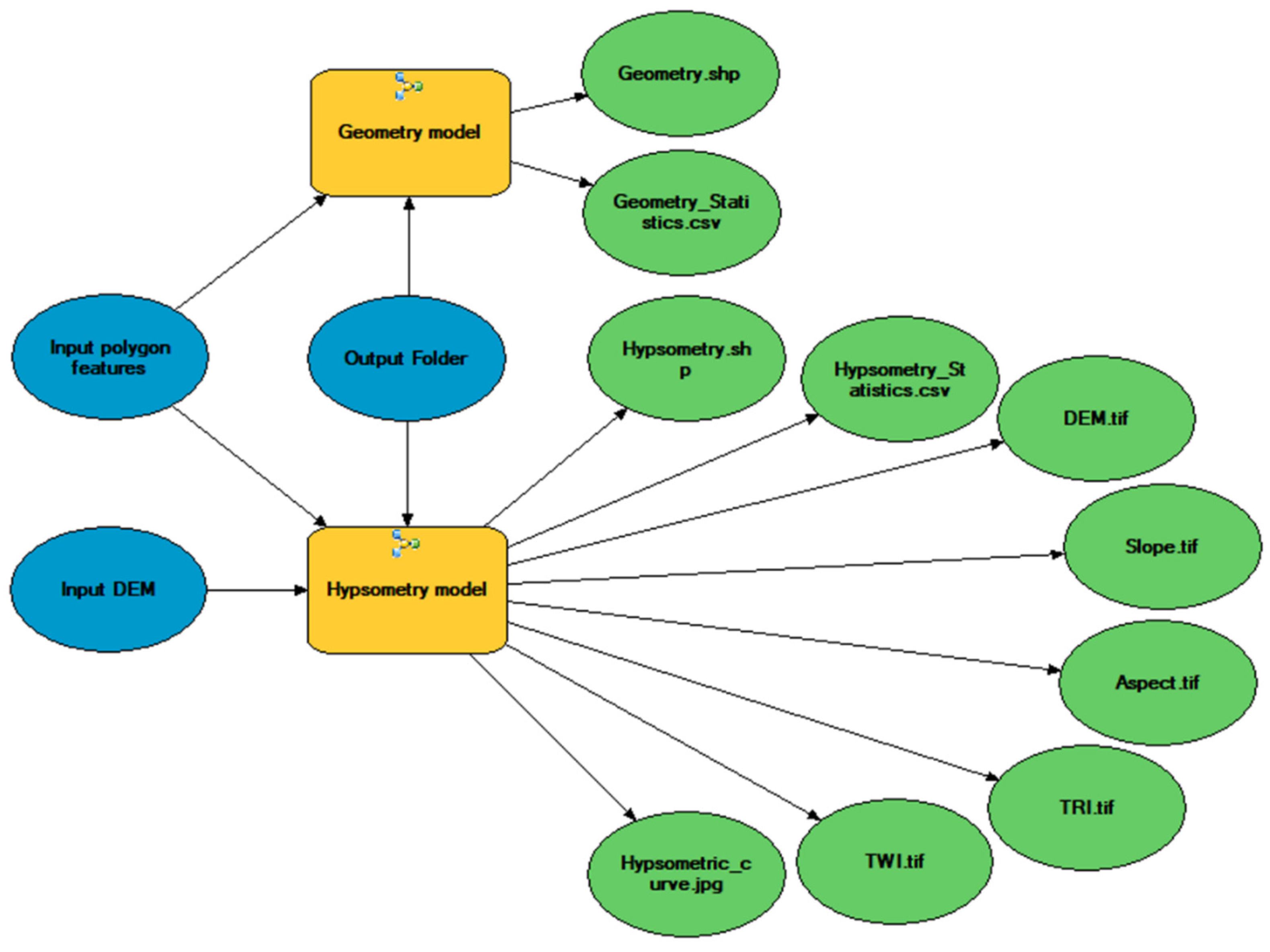
3.2. Description of the Toolbox

The Morphometry Assessment Tools (MAT) toolbox consists of two modules: (a) Geometry and (b) Hypsometry. The modules were developed using the ArcGIS ModelBuilder visual programming language. The schematic workflow for the MAT toolbox presents the input data, main models, and output data in the standard symbology of the ModelBuilder application (Figure 3). The division into modules allows the user to run the computational processes separately depending on which metrics need to be determined. This also allows shortening the computation time if only basic parameters are needed. Individual modules use different extensions of ArcGIS and operate with different levels of detail. The Geometry module can be used for calculations based only on vector analysis tools, while the Hypsometry module requires a license for the Spatial Analyst extension. The toolbox was tested with the ArcGIS 10.7.1. Models are run from the ArcCatalog or ArcToolbox applications as dialogue boxes (Figure 4). The user can also run the models in edit mode; thus, all intermediate data will also be saved. The input data requirements, the algorithms implemented in the models, and the output data are described in detail below.

3.2.1. Input Data Requirements

The first input data set for the analysis is the boundary of the landform. The boundaries should be prepared as polygons and saved as an ESRI Shapefile (.shp) or geodatabase feature class. The boundary line should be situated on the edges of the concave form (Figure 5). The landform edge polygon can be created manually using vectorisation methods based on a digital elevation model, slope map, contour lines, or orthophotos. It is also possible to apply the methods for the semi-automatic delimitation of the edge polygon using, for example, landform classification based on the Topographic Position Index (TPI) [73] or the algorithms used in drainage network extraction, such as sink and depression evaluation and catchment delineation [74]. In this study, data collected from the field measurements were used to determine the form boundaries. Points measured on the highest ridges (so-called break lines) of the analysed forms were used to determine the vertexes of the boundary polygon of each valley. The data were imported to the ArcGIS software using the Add XY Data function. Then the data were converted to the polygon layer using the Points to Line and the Feature to Polygon tools.
The second data set is a digital elevation model such as DEM, DTM, or DSM, which can be prepared in one of the raster data formats accepted by the ArcGIS software (among others, GeoTIFF, ESRI GRID, PNG, or JPG). DEM should cover the form boundary over the entire area and preferably should also include an outside buffer zone. The polygon layer and DEM need to be in the same projected coordinate system with linear units (meters) to perform the correct calculations.

3.2.2. Geometry Module

The module of basic morphometric parameters is based on the geometry of the polygon features. Table 3 presents the names of parameters and formulas used for the calculations as well as the references of the individual characteristics. The selected parameters are the ones that are most commonly used to characterise the geometry of dry concave landforms.
The area (A) and perimeter (P) of the form are calculated using the Python functions based on the coordinate system of the input layer. The length (L) of the form was defined as the length of the long axis of a rectangle that encircles the identified feature, known in the literature as the minimum bounding box [38,75]. The convex hull method was used for the calculation of the minimum bounding box geometry.
The Minimum Bounding Geometry function was used in the calculation of the length (L) and the orientation (O; azimuth of the major axis) of the polygons. In the literature, there are various approaches used for calculating the length of a form. It can be determined, for example, as a line along the main channel to the farthest point on the basin boundary [16]. The results based on the minimum bounding geometry are a simplified calculation method, but it is possible to apply to various forms and also to those in which the channel cannot be determined. The mean form width (W) is calculated by dividing the area by the perimeter of the form [76]. The elongation ratio (Re) is based on the formula presented by Schumm [16], defined as the ratio of the diameter of a circle of the same area as the form to the maximum form length. The value of Re varies from 0 (in a highly elongated shape) to 1 (in a circular shape). The circularity ratio (Rc) is based on the equation proposed by Miller [77] as the ratio of the area of the form to the area of the circle with the same perimeter. Index values below 0.5 indicate the elongation of the form, while values close to 1 indicate a high circularity. The next index is the form’s compactness coefficient (Cc), defined as the ratio of the perimeter of a form to the circumference of the circular area, which equals the area of the form [15]. The form factor (Ff) presented by Horton [76] determines the ratio of the form area to the square of its length. Form factor values are always below 0.754 (for a perfectly circular form); the smaller the values are, the more elongated the form is. The shape factor (Sf) is calculated as the reciprocal of the form factor [77]. The parameters W, Re, Rc, Cc, Ff, and Sf are computed using Python expressions.
All the geometric parameter values calculated for each polygon in the input layer are saved in the attribute table of the new output polygon layer created in the .shp format. Based on the parameter values derived for all features, the descriptive statistics—maximum, mean, minimum, range, and standard deviation—are calculated and saved in the output statistics table in the .csv format. Output files are created in the folder specified by the user. The names of the output files are created automatically starting from the name of the input layer and ending with the “Geometry” and “Geometry_Statistics” suffixes, respectively.

3.2.3. Hypsometry Module

The module of hypsometric parameters is based on the polygon features and the digital elevation model. Table 4 presents the names of the parameters, formulas, and references of the individual indexes. Based on the literature, the selected parameters are commonly used to characterise the hypsometry of concave landforms.
The maximum (Zmax), mean (Zmean), and minimum (Zmin) height and the elevation range (Zrange) values are extracted directly from the DEM layer using the Zonal Statistics function. The Zrange parameter corresponds to the total relief metric. In order to determine the slope values, a slope raster is generated (in degrees; the values range from 0 to 90) [78]. Then, the Zonal Statistics function is applied to calculate the maximum (Smax), mean (Smean), and minimum (Smin) values in the area of each polygon feature. The next tool used in the Hypsometry model is the aspect, which identifies the direction of the downhill slope faces. The values of each cell in the output raster indicate the compass direction the surface faces at that location (clockwise in degrees from 0 due north to 360) [78]. The mean aspect (Amean) parameter is calculated by averaging all values across the entire surface of each form using the Zonal Statistics function. Mean aspect could be a preferred characteristic compared with the orientation (O) parameter when it comes to evaluating the total effect of solar radiation and wind direction on the form distribution [43].
Another spatial index in the Hypsometry module is the terrain ruggedness, which determines the variability or irregularity in elevation (highs and lows) within a sampled terrain unit. For the calculation, the Terrain Ruggedness Index developed by Riley et al. [79] was selected, as it is widely used, but it is not available in the ArcGIS Desktop system tools. TRI expresses the elevation difference between adjacent cells of a DEM. The metric measures the difference in elevation values from a centre cell and the eight cells directly surrounding it. Then, the eight elevation differences are squared and averaged. The square root of this average results is the TRI value for the centre cell. To calculate the TRI raster in the hypsometry model, an algorithm was developed that uses the Focal Statistics function, which is based on the weighted neighbourhood. The ASCII-weighted kernel files were prepared to sequentially calculate the differences between the centre cell and the eight surrounding it. To make the elevation differences positive, the Abs function that calculates the absolute value of the cells was implemented. For the output TRI raster, the Zonal Statistics function was used to determine the values of the maximum (TRImax), mean (TRImean), and minimum (TRImin) values in the area of each polygon feature.
Although the toolbox is intended for dry concave forms, one spatial index was introduced to assess the topographic control on hydrological processes within the form area. The Topographic Wetness Index (TWI) was developed by Beven and Kirkby [80] within TOPMODEL. Among other things, TWI is widely used to identify hydrologic flow paths, but it is still missing in the ArcGIS Desktop system tools. The index is a function of the slope and the upstream contributing area:
TWI = ln (a/tanb)
where:
  • a—upstream contributing area;
  • tanb—local slope in radians.
The index is a number expressed without units, for which higher values indicate the water accumulation areas while lower values represent crests and ridges. The workflow of the TWI raster calculation in the Hypsometry module includes the Slope tool, Hydrology tools, and Math tools. As for the previous spatial indexes, the Zonal Statistics function was used to determine the maximum (TWImax), mean (TWImean), and minimum (TWImin) values in the area of each landform.
The following parameter is the hypsometric integral (HI), which is defined as the area below the hypsometric curve, and it has been used in classifying areas according to their geological stage of development [81]. HI is an indicator of the erosion cycle. The erosion cycle is defined as the total time it takes to denudate a unit of terrain to the level of the base erosion. The erosion cycle can be divided into three stages: monadnock (old) (HI ≤ 0.3), equilibrium state or mature stage (0.3 ≤ HI ≤ 0.6), and inequilibrium or young stage (HI ≥ 0.6). The hypsometric curve used to quantify HI represents the relative proportion of the form area below a given height (Figure 6) [81,82]. The shape of the hypsometric curve is related to its stage of form development. Convex hypsometric curves are typical of a youthful stage, s-shaped curves are related to a mature stage, and concave curves are indicative of a peneplain stage [16,42,81]. The hypsometric curves can also show the dynamic of geomorphological processes [2,83].
In the workflow of the HI parameter calculation, we followed Matos and Dilts [51]. The hypsometric integral is calculated by slicing the area into elevation bands and plotting the cumulative area for each band. Additionally, an algorithm was developed to plot a graph for the hypsometric curve of each analysed landform. For this purpose, a graph template was prepared, which is used in the Make Graph tool in the Hypsometry model.
The last characteristic is the volume (V) of the concave landform. The first step of the analysis is the cover plate raster creation according to the upper edge of the form. The polygon boundary is converted to points based on vertexes. Then, for the points, the elevation values from the DEM are extracted. Using altitude values, the interpolation is performed using the Natural Neighbor algorithm. The choice of the method was preceded by testing other interpolation tools available in the ArcGIS software, such as IDW, Kriging, Spline, Trend, and also the TIN model. It was stated that the Natural Neighbor method gave the most appropriate results—i.e., the interpolated cover surface fitted well to the edge of the form and at the same time was smooth in the interior area (Figure 7). A comparison of the results according to the interpolation method used is presented in the results section of this study.
The second step of the analysis is the estimation of the material volume. The resulting raster is generated from two surfaces: the overlay DEM and the DEM of the form. The volume for each cell is calculated according to the formula:
V = Ap ∗ (Zb − Za)
where:
  • V—volume [m3];
  • Ap—cell area [m2];
  • Zb—cell value of the overlay DEM (before surface);
  • Za—cell value of the DEM (after surface).
The final volume (V) parameter is calculated by summing up all the cells in the area of each form.
All the output files of the Hypsometry module are saved in a folder specified by the user. Output files include an output polygon layer in the .shp format—the parameter values are saved in the attribute table of the layer; an output statistics table in the .csv format—descriptive statistics (maximum, mean, minimum, range, standard deviation) of parameter values calculated for all features in the polygon layer; output raster layers in the GeoTIFF (.tif) format—DEM, Slope, Aspect, TRI, and TWI—clipped to the area of the polygon features; output graphs data in the .jpg and .csv format—hypsometric curves determined for the areas of all polygon features (by FID field) (Figure 8). The names of the output files are created automatically, starting from the name of the polygon input layer and ending with the “Hypsometry”, “Hypsometry_Statistics”, “DEM’, “Slope”, “Aspect”, “TRI”, “TWI”, “Hypsometric_curve” suffixes.

4. Results

4.1. Landform Geometry Assessment

The results calculated with the use of the Geometry module of the MAT toolbox for 21 erosion-denudation valleys are presented in Table 5.
Erosion-denudation valleys show a diversified area (A), ranging from 434.06 m2 (valley 4—Buślarki) to 4161.63 m2 (valley 17—Koprzywno) (mean, 1796.50 m2; std deviation, 1149.36). The length (L) of the forms, which is the result of linear erosion processes taking place at their bottoms [63], does not exceed 150 m. The maximum values were recorded for the valley of Piaski Pomorskie—145.92 m (mean, 88.87 m; std deviation, 31.77). They are generally short forms with a relatively narrow bottom. The mean widths (W) of the valleys range from 8.04 to 37.5 m (mean, 19.09 m; std deviation, 8.23). Compared with other forms of this type occurring in the young glacial area of the Polish Lowlands, these are small forms [84].
The form elongation ratio (Re) ranges from 0.34 to 0.82, with a mean of 0.53 (std deviation, 0.12). The values of the Re correspond very well with the circularity ratio (Rc), proving that most of the studied valleys have a more elongated bottom. The elongation of the form is the result of linear erosion processes occurring along the longitudinal axis [85,86]. In the case of valleys where the Rc value is above 0.5, it can be concluded that longitudinal processes, such as linear erosion, occurred with a similar intensity as transverse processes, such as mass movements, solifluction, and slope wash, responsible for, among other things, widening the bottom of the forms. Such a situation was recorded in the Rymierowo area, where the Rc value for valley 21 is 0.86. This form belongs to the shortest type, as confirmed by the fact that in its development, the longitudinal processes acted with the same intensity as the transverse processes, and the form is at the initial stage of development.
The dimensionless form factor (Ff) represents the ratio of the valley area to the square of its length. Low values of the form factor (Ff) confirm the elongation of forms. In the case of the studied valleys, this factor varies from 0.09 to 0.53 (mean, 0.23; std deviation, 0.11). The dimensionless shape factor (Sf), being the inverse of the form factor, takes the highest values for the most elongated forms. These factor values range from 1.88 to 10.77 (mean, 5.14; std deviation, 2.13).

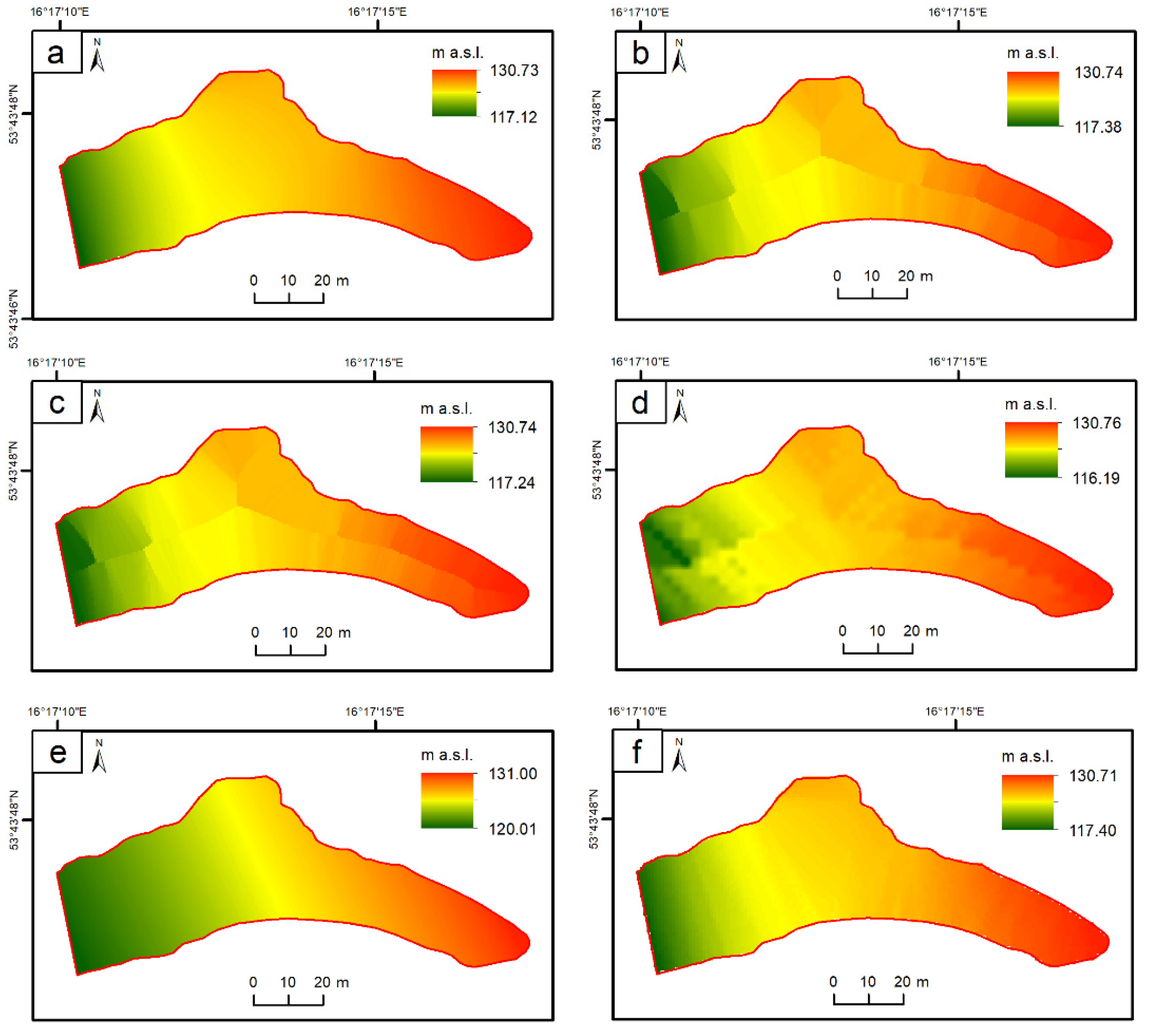
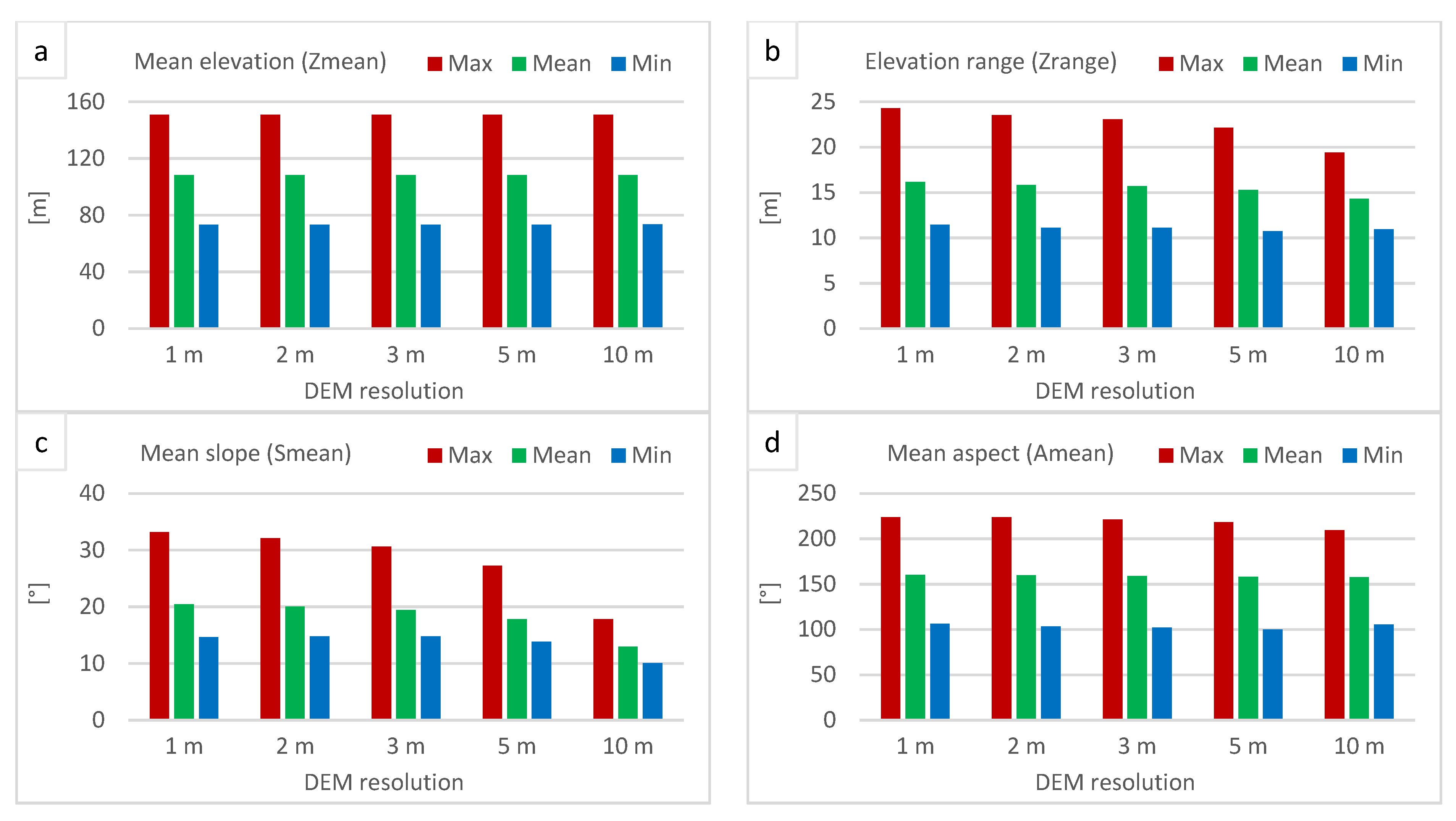
4.2. Landform Hypsometry Assessment

The parameters calculated with the use of the Hypsometry module of the MAT toolbox for 21 erosion-denudation valleys are presented in Table 6.
The elevation range (Zrange) in the 21 analysed valleys, representing the difference in the maximum elevation (Zmax) measured on the valley edge and the minimum elevation (Zmin) at the valley bottom, vary from 4.26 to 24.52 m (mean 11.28, std deviation 5.70). The most considerable elevation differences were recorded for the Koprzywno area, where the Zrange value for the valley Koprzywno 17 is 24.52 m. The lowest value of the Zrange was recorded for the valley Piaski Pomorskie 14 (4.26 m). Low values of the Zrange parameter correspond to a slight variation in the relief of the studied valleys, which may indicate that the role of overland flow in shaping the relief of the valleys was small [84].
The valley side slopes (Smax, Smin) are varied, as the maximum gradient range from 27.85° to 52.04° and the average (Smean) from 11.95° to 34.62°. The highest valley side slopes were recorded for the Koprzywno area (minimum 44.27°, maximum 52.04°) and the smallest for the Buślarki area (minimum 27.85°, maximum 45.27°). Undoubtedly, this is the result of the relief energy of the areas within which the valleys occur. The most considerable differences were observed for the Koprzywno and Rymierowo test areas, reaching over 100 m, while the smallest differences were found in the Buślarki area, amounting to just over 40 m. Similarly, the highest valley side slopes were recorded for the Koprzywno area and the lowest for the Buślarki area. These topographical conditions are conductive to gully erosion processes.
The mean aspect (Amean) parameter values of the valleys indicate the eastern direction in the Buślarki test area, the south direction in the Piaski Pomorskie test area, the southwest direction in the Koprzywno test area, and the southeast direction in the Rymierowo test site. These values are in line with the field observations and aspect maps calculated using the model.
The TRI (TRImax, TRImean, TRImin) values are low and show little variability. This means that the terrain ruggedness in the area of the valleys is low. The side of the valleys are smooth and devoid of irregularity. These results are also determined by the resolution of the DEM data.
The Topographic Wetness Index (TWImax, TWImin) values range from −0.15 to 17.19. The standard deviation of the average (TWImean) and minimum TWI (TWImin) values within all the valleys is small. The close-up values of the TWI index may indicate a similar process of overland flow formation in the analysed forms.
Hypsometric integral (HI) values are within the range of 0.36–0.68, with a mean value of 0.52. The maximum recorded value of 0.68 occurs in the Rymierewo test area and the lowest 0.36 in the Piaski Pomorskie test area. It should be noted that 5 of the 21 analysed valleys show a HI index value of above 0.6, which indicates that they are young forms [81]. The other valleys are in the mature stage of development. Three valleys may be included in the older forms (HI 0.36–0.39). The calculated HI parameter values confirm the shapes of the hypsometric curves (Figure 9a–d). There are 5 convex hypsometric curves that are typical of a youthful stage, 13 s-shaped curves that are related to a middle stage, and 3 concave curves are indicative of an old stage.
The Volume (V) parameter includes the surface of the forms and the elevation range within the forms. Based on this holistic parameter, the results are presented according to the DEM data source (Table 7). The obtained values indicate the significant diversification of the volume from 212.52 to 16,833.17 m3 based on the field data and from 154.13 to 16,809.18 m3 based on the LiDAR data. Within individual research sites, valleys with both small and large volumes of denuded material were identified. The highest volume values were recorded for valley 17 in the Koprzywno test area. The volume of the remaining two valleys, 16 and 18, is close to the average value, as calculated both on the basis of field data and LiDAR data. The lowest volume values were recorded for the Buślarki test area. Among the eight mapped valleys of this area, seven have values below the average, which allows us to state that they are the smallest forms among all the studied valleys.
The differences in the results for the volumetric parameter were at an average level of 12% in comparing the two data sources (Table 7). It should be stated that the calculated volume values based on the LiDAR data are, in most cases, underestimated in relation to the measurements made directly in the field. They are on average 15% lower than those calculated based on field digital elevation models. The valleys determined based on the LiDAR data are shallower in relation to their depth measured in the field. More considerable differences should be noted for the valleys that were particularly elongated, narrow, and deep. It should also be noted that in the case of eight forms, the volume values calculated from the LiDAR data were higher in relation to the field volume. On average, the values that were overestimated differed by 7% from the field data. The most significant differences, in this case, were visible in the Rymierowo area. These valleys are located directly on the shoreline of the lake. They also have the greatest width compared with the other forms.
Comparing the results due to the interpolation method applied to the overlay DEM creation, it can be seen that the average error was 5% (Table 8). The greatest differences are visible in the case of the Trend, Spline, and IDW methods, which excludes them from being used in the adopted calculation procedure. The other methods give very similar results, but the analysis of the spatial distribution of values (Figure 7) supports the use of the Natural Neighbor method.

5. Discussion

5.1. Applicability of the MAT Toolbox for the Morphometric Assessment of the Concave Landforms

The toolbox was tested on an example of 21 erosion-denudation valleys. A large variety of individual morphometric parameters within the same test area was observed, which may indicate that the analysed forms are at different stages of development. Indeed, the formation of the valleys was predisposed to the shape of the area within which the valleys occurred. The development of the landforms was not synchronous on the examined test areas due to a few factors. The most important include: the location of the valleys in geomorphologically different units (morainic uplands, outwash plains), differences in the elevation range of the ridges zones, their different longitudinal and latitudinal orientation, and as a result, differences in the aspect of their slopes. The hypsometric integral (HI) parameter values also indicate different stages of development of the valleys. It should be noticed that for genetically different landforms, such as gullies, different phases of form development were observed [2,8,87]. To test the applicability of the developed procedure on genetically different landforms, the MAT toolbox was applied to the 11 channel heads. The input data (DEM, landforms boundaries) used for calculations were obtained from the research conducted by Mazurek [88]. Channel heads determined by groundwater outflows assume the form of alcoves or niches that dissect slopes to form the headwater depressions [89]. The values of the geometric and hypsometric characteristics calculated using the MAT toolbox were consistent with the range presented by Mazurek [88], which confirms that it is universally applicable. The results are presented in the form of tables, maps, and a graph in the Supplementary Materials (Figures S1 and S2, Tables S1 and S2).
The morphometric parameters of the examined forms may be the basis for their typology and thus may be the basis for the identification of groups of landforms with similar morphometric features.

5.2. Advantages and Limitations of the MAT Toolbox

The methodology presented in the study is an approach based on the automatic extraction of the morphometry of concave landforms. The calculation is based on a minimal set of input data: the form boundaries and the digital elevation model (DEM) of the forms. The morphometric assessment using the presented toolbox can be performed for any type of concave form, regardless of its scale and shape. The calculations did not take into account the parameters related to the drainage network, which are characteristic of the analysis of river basins. This allows the use of algorithms for dry forms, where there are no watercourses, such as dry erosion-denudation valleys, sinkholes, or glacial cirques.
Calculations of the basic parameters are based on the geometry of the form boundary. The length of the form is determined by the minimum bounding box. This is a simplified method, but the form polygon can have a very complicated geometry, unlike in other tools of this type, such as for example the ACME tool [43], which is adapted to glacial cirques with simple geometry. The main watercourse is also not needed for calculations. On the other hand, the width of the form based on the surface-to-length ratio allows for the average value of the entire form to be obtained, and not only on selected cross profiles.
Calculations of the hypsometric parameters are based on the geometry of the form boundary and the digital elevation model. The Hypsometry module contains the tools, which are widely used, but they are not available in the ArcGIS Desktop system tools. These are the following functions: Terrain Ruggedness Index (TRI), Topographic Wetness Index (TWI), hypsometric integral (HI), hypsometric curves, and volume of the concave landform. The results of the mentioned parameters were successfully validated using the independent tools. The TRI parameter values were consistent with the results of the Terrain Ruggedness Index algorithm from the GDAL library available in the QGIS software. The TWI results corresponded with the calculations using the Topographic Wetness Index (TWI) function available in the SAGA GIS software. An important parameter of the presented toolbox compared with other tools of this type is the hypsometric integral (HI) and hypsometric curve graph. The results were successfully validated using the CalHypso script [42]. The volume parameter was validated using the algorithm developed by Báčová et al. [46]. The results were very similar. Minor differences resulted from the different overlay DEM interpolation methods.
The computational time of the MAT toolbox was examined. Calculations of the geometric parameters of the 21 valleys with the mean area of almost 1800 m2 and the mean perimeter of 216 m were made in 4.12 s. Calculations of the hypsometric parameters of the 21 valleys using DEM of 0.5 m resolution were made in 12 min 36 s.
For comparison, the calculation of only one parameter, the volume, based on the same input data in the rillStats tool [46], took 1 h 4 min 14 s. When performing calculations using the MAT tool, it should be taken into account that the time of the hypsometric calculations is dependent on the size and spatial resolution of the input DEM data and also on the computing capabilities of the user computer. High-resolution data may take a longer time to compute.
The toolbox may be improved with new functionalities in the future. An important issue to resolve is the automatic detection of the form boundaries. The implementation of such a function would allow for the elimination of potential errors that may occur on the part of the user during the vectorisation procedure.
In conclusion, the important methodological advantages of the MAT toolbox compared with other tools can be highlighted:
(1)
Comprehensive morphometric assessment using only one tool in one software;
(2)
Minimal set of input data required;
(3)
Automatic extraction of the parameters which are widely used, but not available in the ArcGIS Desktop system tools: Terrain Ruggedness Index (TRI), Topographic Wetness Index (TWI), hypsometric integral (HI), hypsometric curves, and volume of the concave landform;
(4)
User-friendly interface (automatic names of the output files; there is no need to set additional parameters by the user);
(5)
Short computational time;
(6)
Automatic calculation of the descriptive statistics and the output raster layers of the spatial parameters.

5.3. Impact of Data Quality and Resolution

The results obtained with the use of the Morphometry Assessment Tools toolbox depend on the quality of input data. The polygon layer of the form’s boundary may be prepared with the use of various methods, such as the manual vectorisation or semi-automatic extraction of objects. If the form’s boundary is processed manually, there may be slight differences in its location depending on the accuracy and perception of the person who performs the digitisation. Báčová et al. [46] investigated the influence of the position and shape of eight different polygons of vectorised rills boundaries on the volume estimation result. The results showed that the calculated material volume differed depending on the area and shape of the polygons, but the differences were as low as ±4%, which was considered a good result.
The result of the calculations of individual hypsometric parameters may be influenced by the DEM data source, their spatial resolution, and their elevation accuracy. In this study, calculations were based on elevation data collected in the field using the total station measurements and based on the airborne laser scanning data. In the case of data obtained using LiDAR methods, errors may be related to the type of the scanner used and its calibration, the density of scanning points, the type of vegetation in the study area, and the interpolation algorithms used at the stage of data post-processing. In the conducted study the maximum difference in the hypsometric assessment was in the range of 19–38% in a few cases based on the LiDAR data compared with the reference data (Table 7). Based on the acquired LiDAR data specification [66] and the literature on the application of these data in the area of northwest Poland [90], it should be stated that the analysis of the forested small landforms based on these LiDAR data may be limited mainly due to fallen trees and piles of brushwood. These elements may be misinterpreted as the ground [90]. Both high and low levels of vegetation can be found within the studied valleys. Tree branches and windthrows in the bottom of the forms are characteristic in the valleys, where higher values of LiDAR data errors were recorded (valley nos. 4, 10, 11, 14, 15). The volume in these cases was significantly underestimated. The second reason for the differences in the results of the calculations of morphometric parameters is the relatively highly inclined valley side. The underestimation of the volume of gullies based on the LiDAR data was observed also by Perroy [22]. Measurements performed in the field using the total station allowed for the precise filtration of points in terms of their location on the ground, and their acquisition density was higher (7 per m2) than that in the LiDAR data (4–6 per m2). This contributed to a more accurate representation of the relief within the analysed forms.
To determine the influence of the spatial resolution of the used DEMs on the accuracy of the obtained results, analyses were conducted on different DEM cell sizes. The original LiDAR DEM with a resolution of 0.5 m was resampled to a resolution of 1, 2, 3, 5, and 10 m. Because the analysed valleys are very small forms, the calculation based on the coarser cell size of 10 m was possible only for the four biggest valleys (nos. 1, 10, 17, and 19 with an area of more than 3000 m2 and mean width about 30 m). This threshold is related to the procedure for determining the slope, TWI, and TRI layers, where each cell is calculated based on a 3 × 3 cell neighbourhood. The results of the selected hypsometric parameters for four valleys are presented in Figure 10. The analysis was also performed for the nine medium size valleys (with an area of more than 1000 m2) using the resolution up to 5 m and for the eight small size valleys (with an area less than 1000 m2) using the resolution up to 3 m. The results are included in the Supplementary Materials (Figures S3 and S4).
It can be seen that the mean elevation (Figure 10a) increases slightly as we move to coarser resolution from 1 m until 10 m. For the other parameters, the differences are larger. Relatively, the greatest changes should be noted for the TRI (Figure 10e) and Slope (Figure 10c) parameters, which strongly depend on the DEM resolution. The same trend of parameter differences is seen for medium and small valleys (see Supplementary Materials (Figures S3 and S4). It is also worth noting that the differences in parameter values are small in the 1–3 m resolution range. The differences increase substantially when we compare the 1 m and 10 m resolution DEMs. The results indicate the loss of details by resampling the higher resolution DEM to coarser resolution. The results also suggest that if high-resolution DEM is available, it should be used in the MAT toolbox analysis instead of low-resolution DEM.

6. Conclusions

This paper presents tools that consist of sets of algorithms designed and implemented in the ArcGIS software. The functions gathered in the toolbox enable the comprehensive morphometric evaluation of any type of dry concave landform. The assessment parameters include the geometry, hypsometry, and volume of forms, calculating a total of 26 metrics. The results obtained with the toolbox were discussed with the example of 21 dry erosion-denudation valleys located in the young glacial area of the Polish Lowlands.
The calculated characteristics allow for inferences to be made about the stages of development of particular forms, their geomorphological processes, and their classification. This tool can be useful in geomorphological analyses, especially to calculate the hypsometric curves and estimate the volume of material erosion in cases where the original form surface is unknown. The recognised morphological types of erosion-denudation valleys show diversified sizes and reliefs. They represent forms that developed in the edge zones of morainic upland and outwash plains. The morphometric characteristics of the valleys record the stages of their development, thus providing information on the functioning of the processes and the transformations of the relief in the Late Glacial and Holocene periods.
Calculations were based on elevation data measured in the field and LiDAR data. The representation of the relief based on LiDAR data could be disturbed by the presence of vegetation, as well as by the shape of the forms, often narrow and deeply incised. The DEM input to the tool can also come from other remote sensing sources, such as terrestrial laser scanning (TLS) or UAV orthophotos.
The tool can be used for various types of concave terrain forms, regardless of their size and genesis. Morphometric evaluation with the use of an algorithm can be performed for natural and anthropogenic forms, such as open-cast mines or excavations.

Supplementary Materials

The following are available online at https://0-www-mdpi-com.brum.beds.ac.uk/article/10.3390/rs13142810/s1, Source Code S1: MAT. The Morphometry Assessment Tools toolbox (MAT), and User Guide; Figure S1: Location of the headwater depressions in the study area after Mazurek [88].; Table S1: Geometric parameters of the headwater depressions.; Table S2: Hypsometric parameters of the headwater depressions.; Figure S2: An example of a visualisation of the output data (Popielewo 4 test site) of the Hypsometry module: (a) DEM map; (b) Slope map; (c) Aspect map; (d) TRI map; (e) TWI map; (f) Hypsometric curve graph.; Figure S3: Variation in maximum, mean, and minimum of the selected morphometric parameters for 1 m, 2 m, 3 m, 5 m, 10 m LiDAR DEM (based on the medium size valleys): (a) Zmean parameter; (b) Zrange parameter; (c) Smean parameter; (d) Amean parameter; (e) TRImean parameter; (f) TWImean parameter; (g) HI parameter; (h) V parameter.; Figure S4: Variation in maximum, mean, and minimum of the selected morphometric parameters for 1 m, 2 m, 3 m, 5 m, 10 m LiDAR DEM (based on the small size valleys): (a) Zmean parameter; (b) Zrange parameter; (c) Smean parameter; (d) Amean parameter; (e) TRImean parameter; (f) TWImean parameter; (g) HI parameter; (h) V parameter.

Author Contributions

Conceptualisation, J.G. and R.P.; methodology, J.G.; software, J.G.; validation, J.G.; formal analysis, J.G. and R.P.; resources, J.G. and R.P.; writing—original draft preparation, J.G.; writing—review and editing, J.G. and R.P.; visualisation, J.G.; funding acquisition, R.P. All authors have read and agreed to the published version of the manuscript.

Funding

This research was conducted with the financial support of the Faculty of Geographical and Geological Sciences, Adam Mickiewicz University in Poznań, Poland.

Institutional Review Board Statement

Not applicable.

Informed Consent Statement

Not applicable.

Data Availability Statement

Not applicable.

Conflicts of Interest

The authors declare no conflict of interest. The funders had no role in the design of the study; in the collection, analyses, or interpretation of data; in the writing of the manuscript; or in the decision to publish the results.

References

  1. Clarke, J.I. Morphometry from maps. In Essays in Geomorphology; Dury, G.H., Ed.; American Elsevier Publ.: New York, NY, USA, 1966; pp. 235–274. [Google Scholar]
  2. Janicki, G. System Stoku Zmywowego i Jego Modelowanie Statystyczne—Na Przykładzie Wyżyn Lubelsko-Wołyńskich (Wash Slope Systems and Their Statistical Modeling: Case Study from the Lublin-Volhnian Uplands); Wydawnictwo Uniwersytetu Marii Curie-Skłodowskiej: Lublin, Poland, 2016; pp. 1–308, (In English Summary). [Google Scholar]
  3. Pike, R.J. Geomorphometry–progress, practice, and prospect. Z. Geomorphol. Supp. 1995, 101, 221–238. [Google Scholar]
  4. Pike, R.J. Geomorphometry—Diversity in quantitative surface analysis. Prog. Phys. Geog. Earth Environ. 2000, 24, 1–20. [Google Scholar] [CrossRef] [Green Version]
  5. Brzezińska-Wójcik, T. Morfotektonika w Annopolsko-Lwowskim Segmencie Pasa Wyżynnego w Świetle Analizy Cyfrowego Modelu Wysokościowego Oraz Wskaźników Morfometrycznych; Wydawnictwo Uniwersytetu Marii Curie-Skłodowskiej: Lublin, Poland, 2013; pp. 1–397. [Google Scholar]
  6. Jasiewicz, J.; Zwoliński, Z.; Mitasova, H.; Hengl, T. Geomorphometry for Geosciences; Adam Mickiewicz University in Poznań—Institute of Geoecology and Geoinformation, International Society for Geomorphometry: Poznań, Poland, 2015; pp. 1–278. [Google Scholar]
  7. Casali, J.; Giménez, R.; Campo-Bescós, M.A. Gully geometry: What are we measuring? Soil 2015, 1, 509–513. [Google Scholar] [CrossRef] [Green Version]
  8. Kociuba, W.; Janicki, G. Spatiotemporal variability of the channel pattern of high Arctic proglacial rivers. In Fluvial Geomorphology and Riparian Vegetation: Environmental Importance, Functions and Effects on Climate Change; Duncan, N., Ed.; Nova Science Publishers, Inc.: New York, NY, USA, 2015; pp. 53–80. [Google Scholar]
  9. Woronko, B.; Rychel, J.; Karasiewicz, T.M.; Kupryjanowicz, M.; Adamczyk, A.; Fiłoc, M.; Marks, L.; Krzywicki, T.; Pachocka-Szwarc, K. Post-Saalian transformation of dry valleys in eastern Europe: An example from NE Poland. Quarter. Int. 2018, 467, 166–171. [Google Scholar] [CrossRef]
  10. Karasiewicz, T.; Tobojko, L.; Świtoniak, M.; Milewska, K.; Tyszkowski, S. The morphogenesis of erosional valleys in the slopes of the Drwęca valley and the properties of the colluvial infills. Biull. Geogr. Phisical Geogr. Ser. 2019, 16, 5–20. [Google Scholar] [CrossRef] [Green Version]
  11. Kociuba, W.; Janicki, G.; Dyer, J.L. Contemporary changes of the channel pattern and braided gravel-bed flood-plain under rapid small valley glacier recession (Scott River catchment, Spitsbergen). Geomorphology 2019, 328, 79–92. [Google Scholar] [CrossRef]
  12. Schoeneberger, P.J.; Wysocki, D.A. Geomorphic Description System, Version 5.0; Natural Resources Conservation Service, National Soil Survey Center: Lincoln, NE, USA, 2017.
  13. MacMillan, R.A.; Shary, P.A. Chapter 9 Landforms and Landform Elements in Geomorphometry. Dev. Soil Sci. Elsevier 2009, 33, 227–254. [Google Scholar] [CrossRef]
  14. Evans, I.S. Geomorphometry and landform mapping: What is a landform? Geomorphology 2012, 137, 94–106. [Google Scholar] [CrossRef]
  15. Horton, R.E. Erosional Development of Streams and Their Drainage Basins; Hydrophysical Approach to Quantitative Morphology. Geol. Soc. Am. Bull. 1945, 56, 275–370. [Google Scholar] [CrossRef] [Green Version]
  16. Schumm, S.A. Evolution of drainage systems and slopes in badlands at Perth Amboy, New Jersey. GSA Bull. 1956, 67, 597–646. [Google Scholar] [CrossRef]
  17. Strahler, A.N. Quantitative geomorphology of drainage basin and channel networks. In Handbook of Applied Hydrology; Chow, V.T., Ed.; McGraw Hill Book Company: New York, NY, USA, 1964; Section 4–11; pp. 4–76. [Google Scholar]
  18. Casali, J.; Loizu, J.; Campo, M.A.; De Santisteban, L.M.; Alvarez-Mozos, J. Accuracy of methods for field assessment of rill and ephemeral gully erosion. Catena 2006, 67, 128–138. [Google Scholar] [CrossRef]
  19. Castillo, C.; Perez, R.; James, M.R.; Quinton, J.N.; Taguas, E.V.; Gomez, J.A. Comparing the accuracy of several field methods for measuring gully erosion. Soil. Sci. Soc. Am. J. 2012, 76, 1319–1332. [Google Scholar] [CrossRef] [Green Version]
  20. Wu, Y.; Cheng, H. Monitoring of gully erosion on the Loess Plateau of China using a global positioning system. Catena 2005, 63, 154–166. [Google Scholar] [CrossRef]
  21. Hu, G.; Wu, Y.; Liu, B.; Zhang, Y.; You, Z.; Yu, Z. The characteristics of gully erosion over rolling hilly black soil areas of Northeast China. J. Geogr. Sci. 2009, 19, 309–320. [Google Scholar] [CrossRef]
  22. Perroy, R.L.; Bookhagen, B.; Asner, G.P.; Chadwick, O.A. Comparison of gully erosion estimates using airborne and ground-based LiDAR on Santa Cruz Island, California. Geomorphology 2010, 118, 288–300. [Google Scholar] [CrossRef]
  23. Eltner, A.; Baumgart, P.; Maas, H.G.; Faust, D. Multi-temporal UAV data for automatic measurement of rill and interrill erosion on loess soil. Earth Surf. Proc. Land. 2014, 40, 741–755. [Google Scholar] [CrossRef]
  24. Kociuba, W.; Janicki, G.; Rodzik, J.; Stępniewski, K. Comparison of volumetric and remote sensing methods (TLS) for assessing the development of a permanent forested loess gully. Nat. Hazards 2015, 79, 139–158. [Google Scholar] [CrossRef]
  25. Vinci, A.; Brigante, R.; Todisco, F.; Mannocchi, F.; Radicioni, F. Measuring rill erosion by laser scanning. Catena 2015, 124, 97–108. [Google Scholar] [CrossRef]
  26. Goodwin, N.R.; Armston, J.D.; Muir, J.; Stiller, I. Monitoring gully change: A comparison of airborne and terrestrial laser scanning using a case study from Aratula, Queensland. Geomorphology 2017, 282, 195–208. [Google Scholar] [CrossRef]
  27. James, M.R.; Robson, S. Straightforward reconstruction of 3D surfaces and topography with a camera: Accuracy and geoscience application. J. Geophys. Res. 2012, 117, 1–17. [Google Scholar] [CrossRef] [Green Version]
  28. Wang, R.; Zhang, S.; Pu, L.; Yang, J.; Chen, J.; Guan, C.; Wang, Q.; Chen, D.; Fu, B.; Sang, X. Gully erosion mapping and monitoring at multiple scales based on multi-source remote sensing data of the Sancha River catchment, Northeast China. ISPRS Int. J. Geo Inf. 2016, 5, 200. [Google Scholar] [CrossRef] [Green Version]
  29. Gong, C.; Lei, S.; Bian, Z.; Liu, Y.; Zhang, Z.; Cheng, W. Analysis of the Development of an Erosion Gully in an Open-Pit Coal Mine Dump During a Winter Freeze-Thaw Cycle by Using Low-Cost UAVs. Remote Sens. 2019, 11, 1356. [Google Scholar] [CrossRef] [Green Version]
  30. Niculiță, M.; Mărgărint, M.C.; Tarolli, P. Chapter 10—Using UAV and LiDAR data for gully geomorphic changes monitoring. Dev. Earth Surf. Proc. 2020, 23, 271–315. [Google Scholar] [CrossRef]
  31. Vandekerckhove, L.; Poesen, J.; Govers, G. Medium-term gully headcut retreat rates in Southeast Spain determined from aerial photographs and ground measurements. Catena 2003, 50, 329–352. [Google Scholar] [CrossRef]
  32. Bouchnak, H.; Felfoul, M.S.; Boussema, M.R.; Snane, M.H. Slope and rainfall effects on the volume of sediment yield by gully erosion in the Souar lithologic formation (Tunisia). Catena 2009, 78, 170–177. [Google Scholar] [CrossRef]
  33. Frankl, A.; Poesen, J.; Scholiers, N.; Jacob, M.; Haile, M.; Deckers, J.; Nyssen, J. Factors controlling the morphology and volume (V)–length (L) relations of permanent gullies in the northern Ethiopian Highlands. Earth Surf. Proc. Land. 2013, 38, 1672–1684. [Google Scholar] [CrossRef] [Green Version]
  34. Stöcker, C.; Eltner, A.; Karrasch, P. Measuring gullies by synergetic application of UAV and close range photogrammetry—A case study from Andalusia, Spain. Catena 2015, 132, 1–11. [Google Scholar] [CrossRef]
  35. James, L.A.; Watson, D.G.; Hansen, W.F. Using LiDAR data to map gullies and headwater streams under forest canopy: South Carolina, USA. Catena 2007, 71, 132–144. [Google Scholar] [CrossRef]
  36. Evans, M.; Lindsay, J.B. High resolution quantification of gully erosion in upland peatlands at the landscape scale. Earth Surf. Proc. Land. 2010, 35, 876–886. [Google Scholar] [CrossRef]
  37. Wu, H.; Zu, X.; Zheng, F.; Qin, C.; He, X. Gully morphological characteristics in the loess hilly-gully region based on 3D laser scanning technique. Earth Surf. Proc. Land. 2018, 43, 1701–1710. [Google Scholar] [CrossRef]
  38. Zumpano, V.; Pisano, L.; Parise, M. An integrated framework to identify and analyze karst sinkholes. Geomorphology 2019, 332, 213–225. [Google Scholar] [CrossRef]
  39. Kociuba, W.; Janicki, G.; Rodzik, J. 3D laser scanning as a new tool of assessment of erosion rates in forested lo-ess gullies (case study: Kolonia Celejów, Lublin Upland). Ann. Univ. Mariae Curie Sklodowska 2014, 69, 107–116. [Google Scholar]
  40. Wells, R.R.; Momm, H.G.; Bennett, S.J.; Gesch, K.R.; Dabney, S.M.; Cruse, R.; Wilson, G.V. A measurement method for rill and ephemeral gully erosion assessments. Soil Sci. Soc. Am. J. 2016, 80, 203–214. [Google Scholar] [CrossRef]
  41. Kociuba, W. Different Paths for Developing Terrestrial LiDAR Data for Comparative Analyses of Topographic Surface Changes. Appl. Sci. 2020, 10, 7409. [Google Scholar] [CrossRef]
  42. Pérez-Peña, J.V.; Azañón, J.M.; Azor, A. CalHypso: An ArcGIS extension to calculate hypsometric curves and their statistical moments. Applications to drainage basin analysis in SE Spain. Comput. Geosci. 2009, 35, 1214–1223. [Google Scholar] [CrossRef]
  43. Spagnolo, M.; Pellitero, R.; Barr, I.D.; Ely, J.C.; Pellicer, X.M.; Rea, B.R. ACME, a GIS tool for Automated Cirque Metric Extraction. Geomorphology 2017, 278, 280–286. [Google Scholar] [CrossRef] [Green Version]
  44. Gafeira, J.; Dolan, M.F.J.; Monteys, X. Geomorphometric Characterization of Pockmarks by Using a GIS-Based Semi-Automated Toolbox. Geosciences 2018, 8, 154. [Google Scholar] [CrossRef] [Green Version]
  45. Jose, C.; Thomas, J.; Prasannakumar, V.; Reghunath, R. BaDAM Toolbox: A GIS-Based Approach for Automated Drainage Basin Morphometry. J. Indian Soc. Remote Sens. 2018, 47, 467–478. [Google Scholar] [CrossRef]
  46. Báčová, M.; Krása, J.; Devátý, J.; Kavka, P. A GIS method for volumetric assesments of erosion rills from digital surface madels. Eur. J. Remote Sens. 2019, 52, 96–107. [Google Scholar] [CrossRef] [Green Version]
  47. Rahmati, O.; Samadi, M.; Shahabi, H.; Azareh, A.; Rafiei-Sardooi, E.; Alilou, H.; Melesse, A.M.; Pradhan, B.; Chapi, K.; Shirzadi, A. SWPT: An automated GIS-based tool for prioritization of sub-watersheds based on morphometric and topo-hydrological factors. Geosci. Front. 2019, 10, 2167–2175. [Google Scholar] [CrossRef]
  48. Arabameri, A.; Asadi Nalivan, O.; Saha, S.; Roy, J.; Pradhan, B.; Tiefenbacher, J.P.; Thi Ngo, P.T. Novel Ensemble Approaches of Machine Learning Techniques in Modeling the Gully Erosion Susceptibility. Remote Sens. 2020, 12, 1890. [Google Scholar] [CrossRef]
  49. Šiljeg, A.; Domazetović, F.; Marić, I.; Lončar, N.; Panđa, L. New Method for Automated Quantification of Vertical Spatio-Temporal Changes within Gully Cross-Sections Based on Very-High-Resolution Models. Remote Sens. 2021, 13, 321. [Google Scholar] [CrossRef]
  50. Villaça, C.V.N.; Crósta, A.P.; Grohmann, C.H. Morphometric Analysis of Pluto’s Impact Craters. Remote Sens. 2021, 13, 377. [Google Scholar] [CrossRef]
  51. Matos, A.; Dilts, T.E. Hypsometric Integral Toolbox for ArcGIS. University of Nevada Reno. Available online: https://www.arcgis.com/home/item.html?id=23a2dd9d127f41c195628457187d4a54 (accessed on 6 April 2021).
  52. Wheaton, J.M.; Brasington, J.; Darby, S.E.; Sear, D.A. Accounting for uncertainty in DEMs from repeat topographic surveys: Improved sediments budgest. Earth Surf. Proc. Land. 2009, 35, 136–156. [Google Scholar] [CrossRef]
  53. Gessesse, G.D.; Fuchs, H.; Mansberger, R.; Klik, A.; Rieke-Zapp, D.H. Assessment of erosion, deposition and rill development on irregular soil surfaces using close range digital photogrammetry. Photogramm. Rec. 2010, 25, 299–318. [Google Scholar] [CrossRef]
  54. Lu, X.; Li, Y.; Washington-Allen, R.A.; Li, Y.; Li, H.; Hu, Q. The effect of grid size on the quantification of erosion, deposition, and rill network. Int. Soil Water Conserv. Res. 2017, 5, 241–251. [Google Scholar] [CrossRef]
  55. Pelletier, J.D.; Orem, C.A. How do sediment yields from post-wildfire debris-laden flows depend on terrain slope, soil burn severity class, and drainage basin area? Insights from airborne-LiDAR change detection. Earth Surf. Proc. Land. 2014, 39, 1822–1832. [Google Scholar] [CrossRef]
  56. Heckmann, T.; Vericat, D. Computing spatially distributed sediment delivery ratios: Inferring functional sediment connectivity from repeat high-resolution digital elevation models. Earth Surf. Proc. Land. 2018, 43, 1547–1554. [Google Scholar] [CrossRef]
  57. Mora, O.E.; Lenzano, M.G.; Toth, C.K.; Grejner-Brzezinska, D.A.; Fayne, J.V. Landslide Change Detection Based on Multi-Temporal Airborne LiDAR-Derived DEMs. Geosciences 2018, 8, 23. [Google Scholar] [CrossRef] [Green Version]
  58. Kaspark, A.; Caster, J.; Bangen, S.G.; Sankey, J.B. Geomorphic process from topographic form: Automating the interpretation of repeat survey data in river valleys. Earth Surf. Proc. Land. 2017, 42, 1872–1883. [Google Scholar] [CrossRef]
  59. D’Oleire-Oltmanns, S.; Marzolff, I.; Peter, K.D.; Ries, J.B. Unmanned aerial vehicle (UAV) for monitoring soil erosion in Morocco. Remote Sens. 2012, 4, 3390–3416. [Google Scholar] [CrossRef] [Green Version]
  60. Marks, L. Timing of the Late Vistulian (Weischselian) glacial phases in Poland. Quat. Sci. Rev. 2012, 44, 81–88. [Google Scholar] [CrossRef]
  61. Karczewski, A. Morfogeneza Strefy Marginalnej Fazy Pomorskiej na Obszarze Lobu Parsęty w Vistulianie (Pomorze Środkowe) (Morphogenesis of the Pomeranian Phase Marginal Zone in the Parseta Lobe Region in the Vistulian (Middle Pomerania)); Wyd. Nauk. UAM Seria Geografia 44: Poznań, Poland, 1989; pp. 1–48. (In Polish) [Google Scholar]
  62. Starkel, L. Geografia Polski. Środowisko Przyrodnicze; Wyd. Nauk. PWN: Warszawa, Poland, 1991; pp. 1–670. (In Polish) [Google Scholar]
  63. Paluszkiewicz, R. Postglacjalna Ewolucja Dolinek Erozyjno-Denudacyjnych w Wybranych Strefach Krawędziowych Pojezierza Zachodniopomorskiego (Postglacial Evolution of Erosional-Denudational Valleys in Selected Scarp Zones of the West Pomeranian Lakeland); Bogucki Wydawnictwo Naukowe: Poznań, Poland, 2016; pp. 1–225, (In English Summary). [Google Scholar]
  64. Dobracka, E. Objaśnienia do Szczegółowej Mapy Geologicznej Polski w Skali 1:50 000; Arkusz Połczyn Zdrój (158): Warszawa, Poland, 2017; pp. 1–71. [Google Scholar]
  65. Head Office of Geodesy and Cartography. GUGiK Data PZGiK. Available online: http://www.gugik.gov.pl/pzgik (accessed on 6 April 2021).
  66. ISOK—IT System of the Country’s Protection. Available online: https://isok.gov.pl/ (accessed on 6 April 2021).
  67. ASPRS. LAS Specification. Version 1.2; The American Society for Photogrammetry & Remote Sensing: Bethesda, MD, USA, 2008; pp. 1–13. [Google Scholar]
  68. Axelsson, P. Processing of laser scanner data—Algorithms and applications. ISPRS J. Photogramm. Remote Sens. 1999, 54, 138–147. [Google Scholar] [CrossRef]
  69. Kurczyński, Z.; Stojek, E.; Cisło-Lesicka, U. Zadania GUGiK realizowane w ramach projektu ISOK. In Podręcznik Dla Uczestników Szkoleń z Wykorzystania Produktów LiDAR; Wężyk, P., Ed.; Główny Urząd Geodezji i Kartografii: Warszawa, Poland, 2015; pp. 22–58. (In Polish) [Google Scholar]
  70. LAS Dataset to Raster Function—Help ArcGIS for Desktop. Available online: https://desktop.arcgis.com/en/arcmap/10.7/manage-data/raster-and-images/las-dataset-to-raster-function.htm (accessed on 6 April 2021).
  71. Creating Raster DEMs and DSMs from Large Lidar Point Collections—Help ArcGIS Desktop. Available online: https://desktop.arcgis.com/en/arcmap/10.7/manage-data/las-dataset/lidar-solutions-creating-raster-dems-and-dsms-from-large-lidar-point-collections.htm (accessed on 6 April 2021).
  72. Dawid, W.; Pokonieczny, K. Analysis of the Possibilities of Using Different Resolution Digital Elevation Models in the Study of Microrelief on the Example of Terrain Passability. Remote Sens. 2020, 12, 4146. [Google Scholar] [CrossRef]
  73. Jenness, J.; Brost, B.; Beier, P. Land Facet Corridor Designer: Extension for ArcGIS. Jenness Enterprises. 2011. Available online: http://www.jennessent.com/arcgis/land_facets.htm (accessed on 6 April 2021).
  74. ESRI Arc Hydro Tools—Tutorial, Version 2; Environmental Systems Research Institute: New York, NY, USA, 2011.
  75. Kobal, M.; Bertoncelj, I.; Pirotti, F.; Dakskobler, I.; Kutnar, L. Using lidar data to analyse sinkhole characteristics relevant for understory vegetation under forest cover—case study of a high karst area in the Dinaric mountains. PLoS ONE 2015, 10, e0122070. [Google Scholar] [CrossRef] [PubMed] [Green Version]
  76. Horton, R.E. Drainage-basin characteristic. Eos Trans. Am. Geophys. Union 1932, 13, 350–361. [Google Scholar] [CrossRef]
  77. Miller, V.C. A Quantitative Geomorphic Study of Drainage Basin Characteristics in the Clinch Mountain Area, Virginia and Tennessee; Office of Naval Research, Technical Report 3; Department of Geology, Columbia University: New York, NY, USA, 1953; p. 51. [Google Scholar]
  78. Burrough, P.A.; McDonell, R.A. Principles of Geographical Information Systems, 2nd ed.; Oxford University Press: New York, NY, USA, 1998; pp. 1–190. [Google Scholar]
  79. Riley, S.J.; DeGloria, S.D.; Elliot, R. A terrain ruggedness index that quantifies topographic heterogeneity. Intermt. J. Sci. 1999, 5, 23–27. [Google Scholar]
  80. Beven, K.J.; Kirkby, M.J. A physically based, variable contributing area model of basin hydrology / Un modèle à base physique de zone d’appel variable de l’hydrologie du bassin versant. Hydrol. Sci. Bull. 1979, 24, 43–69. [Google Scholar] [CrossRef] [Green Version]
  81. Strahler, A.N. Hypsometric (area-altitude) analysis of erosional topography. GSA Bull. 1952, 63, 1117–1142. [Google Scholar] [CrossRef]
  82. Pike, R.J.; Wilson, S.E. Elevation–relief ratio, hypsometric integral and geomorphic area–altitude analysis. GSA Bull. 1971, 82, 1079–1084. [Google Scholar] [CrossRef]
  83. Jahn, A. Morphological slope evolution by linear and surface degradation. Geogr. Pol. 1968, 14, 9–22. [Google Scholar]
  84. Majewski, M.; Paluszkiewicz, R. The origin and evolution of small dry valleys in the last-glacial area on the example of the Pomeranian Lake District (Poland). Est. J. Earth Sci. 2019, 68, 26–36. [Google Scholar] [CrossRef]
  85. Gregory, K.J.; Walling, D.E. Drainage Basin: Form and Processes; Edward Arnold: London, UK, 1973; pp. 1–458. [Google Scholar]
  86. Mazurek, M. Hydrogeomorfologia Obszarów Źródliskowych (Dorzecze Parsęty, Polska NW). Hydrogeomorphology of Channel Heads (the Parseta Drainage Basin, Nw Poland); Adam Mickiewicz University Press: Poznań, Poland, Seria Geografia 92; 2010; pp. 1–304, (In English Summary). [Google Scholar]
  87. Mazaeva, O.; Pelinen, V.; Janicki, G. Development of bank gullies on the shore zone of the Bratsk Reservoir (Russia). Ann. Univ. Mariae Curie Sklodowska 2014, 69, 117–133. [Google Scholar] [CrossRef] [Green Version]
  88. Mazurek, M. Morphometric differences in channel heads in a postglacial zone (Parsęta catchment, West Pomerania). Quest. Geogr. 2006, 25A, 39–47. [Google Scholar]
  89. Mazurek, M. Geomorphological processes in channel heads initiated by groundwater outflows (the Parsęta catchment, north-western Poland). Quaest. Geogr. 2011, 30, 33–45. [Google Scholar] [CrossRef] [Green Version]
  90. Pawleta, M.; Zapłata, R. Nieinwazyjne Rozpoznanie Zasobów Dziedzictwa Archeologicznego: Potencjał i Możliwości; Uniwersytet im. A. Mickiewicza w Poznaniu, Fundacja “5Medium”, E-Naukowiec: Poznań, Poland, 2015; pp. 1–329. (In Polish) [Google Scholar]
Figure 1. Location of the study area: (a) Buślarki test area; (b) Piaski Pomorskie test area; (c) Koprzywno test area; (d) Rymierowo test area.
Remotesensing 13 02810 g001
Figure 2. An example of an erosion-denudation valley (Koprzywno test area, valley no. 16): (a) Field photo of the valley; (b) Digital elevation model of the valley based on the field measurements.
Remotesensing 13 02810 g002
Figure 3. The schematic workflow for the MAT toolbox.
Remotesensing 13 02810 g003
Figure 4. The interface of the MAT toolbox.
Remotesensing 13 02810 g004
Figure 5. Example of the boundary of the concave landform: (a) Hillshade map of the valley; (b) DEM of the valley based on the LiDAR data.
Remotesensing 13 02810 g005
Figure 6. Hypsometric curve after Strahler [81]. The area of the region under a curve (R) is a hypsometric integral. A hypsometric curve is represented by function f(x), where the total elevation (H) is relief within the area (maximum elevation minus minimum elevation), total area (A) is the total surface area, and area (a) is the surface area above a given altitude (h).
Remotesensing 13 02810 g006
Figure 7. Comparison of various methods for the interpolation of the overlay surface: (a) Natural Neighbor method; (b) IDW method; (c) Kriging method; (d) Spline method; (e) Trend method; (f) TIN method.
Remotesensing 13 02810 g007
Figure 8. An example of a visualisation of the output data of the Hypsometry module: (a) DEM map; (b) Slope map; (c) Aspect map; (d) TRI map; (e) TWI map; (f) Hypsometric curve graph; (g) Attribute table of the output layer; descriptive statistics output table.
Remotesensing 13 02810 g008
Figure 9. Hypsometric curves of the erosion-denudation valleys: (a) Buślarki test area; (b) Piaski Pomorskie test area; (c) Koprzywno test area; (d) Rymierowo test area.
Remotesensing 13 02810 g009aRemotesensing 13 02810 g009b
Figure 10. Variation in maximum, mean, and minimum of the selected hypsometric parameters for 1 m, 2 m, 3 m, 5 m, 10 m LiDAR DEM (based on the large size valleys): (a) Zmean parameter; (b) Zrange parameter; (c) Smean parameter; (d) Amean parameter; (e) TRImean parameter; (f) TWImean parameter; (g) HI parameter; (h) V parameter.
Remotesensing 13 02810 g010aRemotesensing 13 02810 g010b
Table 1. Morphometric parameters implemented in the ArcGIS open-source tools for the concave forms analysis.
ToolMorphometric Parameters
AreaPerimeterLengthWidthOrientationElongation RatioCircularity RatioCompactness CoefficientForm FactorElevationSlopeAspectTRITWIHIVolume
CalHypso [42] ×
ACME [43]××××× × ××× ×
BaDAM [44]×××× ××××× ×
rillStats [46] ×
SWPT [47]×××× ×××× ×
Hypsometric Integral Toolbox [51] ×
Table 2. Hypsometric characteristics of the test areas.
Test AreaHypsometric Parameters
Minimum Elevation (m a.s.l.)Maximum Elevation (m a.s.l.)Elevation Range (m)Maximum Slope (°)Mean Slope (°)
Buślarki56.2121.965.751.07.1
Piaski Pomorskie69.9144.374.462.35.9
Koprzywno80.3159.879.556.76.8
Rymierowo141.5164.222.746.54.2
Table 3. Definitions of geometric parameters.
Geometric ParametersUnitsFormulaReferences
Area (A)(m2)The projected area enclosed by form boundary
Perimeter (P)(m)Length of the horizontal projection of form boundary
Length (L)(m)Length of the long axis
Width (W)(m)W = A/L[76]
Orientation (O)(°)Orientation (azimuth) of the long axis
Elongation ratio (Re)(-) Re = 1.128 A /L[16]
Circularity ratio (Rc)(-)Rc = 4πA/P2[77]
Compactness coefficient (Cc)(-) Cc = 0.282 P / A [15]
Form factor (Ff)(-)Ff = A/L2[76]
Shape Factor (Sf)(-)Sf = 1/Ff[77]
Table 4. Definition of hypsometric parameters.
Hypsometric ParametersUnitsFormulaReferences
Maximum elevation (Zmax)(m)Maximum elevation from DEM
Mean elevation (Zmean)(m)Mean elevation from DEM
Minimum elevation (Zmin)(m)Minimum elevation from DEM
Elevation range (Zrange)(m)Zrange = Zmax − Zmin
Maximum slope (Smax)(°)Maximum slope calculated from DEM[78]
Mean slope (Smean)(°)Mean slope calculated from DEM[78]
Minimum slope (Smin)(°)Minimum slope calculated from DEM[78]
Mean aspect (Amean)(°)Mean aspect calculated from DEM[78]
Maximum Terrain Ruggedness Index (TRImax)(m)Maximum Terrain Ruggedness Index calculated from DEM[79]
Mean Terrain Ruggedness Index (TRImean)(m)Mean Terrain Ruggedness Index calculated from DEM[79]
Minimum Terrain Ruggedness Index (TRImin)(m)Minimum Terrain Ruggedness Index calculated from DEM[79]
Maximum Topographic Wetness Index (TWImax)(-)Maximum Topographic Wetness Index calculated from DEM[80]
Mean Topographic Wetness Index (TWImean)(-)Mean Topographic Wetness Index calculated from DEM[80]
Minimum Topographic Wetness Index (TWImin)(-)Minimum Topographic Wetness Index calculated from DEM[80]
Hypsometric integral (HI)(-) HI = Z m e a n Z m i n Z m a x Z m i n [81,82]
Volume (V)(m3)V = A p × ( Z b   Z a )
Ap—cell area
Zb—cell value of the overlay DEM (before surface)
Za—cell value of the DEM (after surface)
Table 5. Geometric parameters of the erosion-denudation valleys.
Test AreaValleyGeometric Parameters
A
Area (m2)
P
Perimeter (m)
L
Length (m)
W
Width (m)
O
Orientation (°)
Re
Elongation Ratio (-)
Rc
Circularity Ratio (-)
Cc
Compactness Coefficient (-)
Ff
Form Factor (-)
Sf
Shape Factor (-)
Buślarki13529.01286.23122.1028.90107.500.550.541.360.244.22
2457.07125.3456.858.0495.300.420.371.650.147.07
31019.36222.39104.789.73103.100.340.261.960.0910.77
4434.06106.1239.9810.86124.300.590.481.440.273.68
52637.33389.97145.9218.0791.000.400.222.140.128.07
6681.23136.0257.6611.8185.600.510.461.470.204.88
71588.49266.74110.4914.38106.800.410.281.890.137.69
82372.08251.17112.1621.15104.100.490.471.450.195.30
Piaski Pomorskie91368.46208.6294.3214.51170.900.440.401.590.156.50
103565.03260.5495.0237.52140.300.710.661.230.392.53
111476.07207.7885.4817.2725.700.510.431.530.204.95
12887.51138.5552.5416.8912.000.640.581.310.323.11
13971.33212.9974.7113.00129.300.470.271.930.175.75
14775.84146.1363.4012.2425.600.500.461.480.195.18
152015.84267.09109.8618.3558.300.460.361.680.175.99
Koprzywno162557.94283.54122.8420.8247.500.460.401.580.175.90
174161.63330.26142.8829.1374.800.510.481.440.204.91
181649.22180.3779.2620.8183.000.580.641.250.263.81
Rymierowo193607.61262.8296.5237.38124.400.700.661.230.392.58
201124.03146.1159.5018.89127.700.640.661.230.323.15
21847.35111.4239.8921.24155.700.820.861.080.531.88
StatisticsMax4161.63389.97145.9237.52170.900.820.862.140.5310.77
Mean1796.50216.2088.8719.0994.900.530.471.520.235.14
Min434.06106.1239.898.0412.000.340.221.080.091.88
Std1149.3676.8931.778.2342.820.120.160.280.112.13
Table 6. Hypsometric parameters of the erosion-denudation valleys.
Test AreaValleyHypsometric Parameters
Zmax
Maximum
Elevation (m)
Zmean
Mean Elevation (m)
Zmin
Minimum Elevation (m)
Zrange
Elevation Range (m)
Smax
Maximum Slope (°)
Smean
Mean Slope (°)
Smin
Minimum Slope (°)
Amean
Mean Aspect (°)
TRImax
Maximum TRI (m)
TRImean
Mean TRI (m)
TRImin
Minimum TRI (m)
TWImax
Maximum TWI (-)
TWImean
Mean
TWI (-)
TWImin
Minimum TWI (-)
HI
Hypsometric Integral (-)
Buślarki178.0673.2764.5713.4933.2414.200.20109.960.500.210.0210.423.200.550.64
278.5374.5669.958.5830.9517.322.52112.920.480.270.108.412.770.620.53
381.7376.1170.5711.1632.9714.350.78108.730.510.230.049.852.990.580.49
481.4078.6775.875.5327.8513.972.95139.810.410.220.087.992.770.710.50
582.3575.9067.0915.2645.2721.370.46122.070.800.350.0511.212.560.120.57
680.9677.3673.407.5637.9018.363.69112.710.580.290.088.902.600.340.52
781.2174.7166.8414.3736.5816.330.78115.490.560.250.0410.422.830.410.54
880.9975.2569.4111.5842.1216.800.82103.150.720.260.0313.512.840.160.50
Piaski Pomorskie9100.9992.8383.0617.9336.5319.953.33169.720.570.310.069.062.720.320.54
10100.6292.1884.9715.6539.1717.420.20166.600.640.250.0211.943.070.330.46
11103.81101.6697.845.9737.0011.950.43185.870.580.180.0210.993.270.350.64
12100.6097.5193.996.6143.3822.311.47181.890.750.360.069.542.390.060.54
1395.1991.4987.527.6738.2420.361.23145.520.560.300.049.952.560.410.54
1498.4895.3494.224.2640.5616.930.10202.810.630.230.0117.193.260.230.37
15102.5498.6196.705.8440.8715.370.10233.240.670.220.0113.573.300.140.36
Koprzywno16129.08117.25105.1623.9252.0434.622.49226.440.950.560.0610.472.11−0.110.50
17128.74116.56104.2224.5250.9533.672.02222.430.960.530.1210.912.27−0.150.50
1894.9190.2085.239.6844.2722.840.62222.710.750.350.0212.872.540.090.51
Rymierowo19157.76150.84146.3211.4438.1516.821.26144.230.600.240.0211.373.160.310.39
20159.41156.51151.228.1943.1924.440.10134.170.730.390.0111.852.470.120.64
21158.11155.71150.437.6834.4616.400.23140.080.510.240.027.892.640.400.68
StatisticsMax159.41156.51151.2224.5252.0434.623.69233.240.960.560.1217.193.300.710.68
Mean103.5998.2292.3111.2839.3219.321.23157.170.640.300.0410.872.780.290.52
Min78.0673.2764.574.2627.8511.950.10103.150.410.180.017.892.11−0.150.36
Std27.1426.8626.945.706.035.861.1544.000.150.100.032.180.340.230.09
Table 7. Volumetric parameter of the erosion-denudation valleys.
Test AreaValleyVolumetric Parameter
V Volume (m3)
Based on the Field Data
V Volume (m3)
Based on the LiDAR Data
V Error
(%)
Buślarki15077.815020.97−1.12
2243.10212.30−12.67
3553.97489.15−11.70
4212.52154.13−27.47
53614.323728.283.15
6600.72557.98−7.11
71222.371229.120.55
82931.813035.103.52
Piaski Pomorskie91584.981532.78−3.29
1011,637.237257.00−37.64
111864.291506.53−19.19
121331.841187.95−10.80
131215.011219.490.37
141212.70920.31−24.11
153674.792376.38−35.33
Koprzywno163732.903769.400.98
1716,833.1716,809.18−0.14
183244.133116.72−3.93
Rymierowo1912,908.4013,967.698.21
202146.142392.7911.49
21232.69305.4931.29
Table 8. Volumetric parameter according to the overlay DEM interpolation method.
Test AreaValleyVNaturalNeighborVIDWVIDW Error (%)VKRIGINGVKRIGING Error (%)VSPLINEVSPLINE Error (%)VTRENDVTREND Error (%)VTINVTIN Error (%)
Buślarki15077.815202.732.465228.722.975321.724.805963.8317.454756.05−6.34
2243.10219.90−9.54242.39−0.29236.67−2.64278.8414.70225.38−7.29
3553.97527.22−4.83552.86−0.20546.52−1.34640.1815.56598.368.01
4212.52183.74−13.54209.65−1.35215.671.48228.267.41227.587.09
53614.323569.90−1.233604.20−0.283633.830.543886.427.533658.121.21
6600.72604.460.62610.571.64663.9510.53653.878.85616.902.69
71222.371123.79−8.061216.11−0.511260.273.101298.926.261168.92−4.37
82931.813060.274.383008.402.613044.853.863021.893.072942.230.36
Piaski Pomorskie91584.981555.28−1.871584.70−0.021613.411.791827.0915.281576.29−0.55
1011,637.239623.34−17.3111,295.39−2.9411,711.670.6410,893.41−6.3911,921.412.44
111864.291678.19−9.981867.580.182083.0111.731535.24−17.651912.482.58
121331.841269.38−4.691310.65−1.591341.300.711284.05−3.591313.75−1.36
131215.011184.28−2.531194.35−1.701241.642.191242.052.231205.81−0.76
141212.701197.52−1.251229.151.361426.4817.631316.618.571154.62−4.79
153674.793703.620.783625.00−1.364294.2416.863549.13−3.423738.131.72
Koprzywno163732.903716.31−0.443720.15−0.344053.438.593611.89−3.243739.190.17
1716,833.1716,249.21−3.4716,611.01−1.3218,291.738.6617,519.124.0716,622.86−1.25
183244.133059.52−5.693248.730.143169.06−2.313431.495.783253.140.28
Rymierowo1912,908.4011,086.76−14.1112,009.05−6.9715,025.1216.4015,020.4616.3612,728.45−1.39
202146.142226.963.772182.221.682228.423.832279.446.212146.220.00
21232.69247.006.15229.44−1.40273.3117.46272.6217.16199.29−14.35
Publisher’s Note: MDPI stays neutral with regard to jurisdictional claims in published maps and institutional affiliations.

