
Seismic Ambient Noise Imaging of a Quasi-Amagmatic Ultra-Slow Spreading Ridge
by
 , and
, and
Mohamadhasan Mohamadian Sarvandani
1,*, 
Emanuel Kästle
2,
Lapo Boschi
1,3,4,
Sylvie Leroy
1 and
Mathilde Cannat
5 1
Institut des Sciences de la Terre Paris, Sorbonne Université, CNRS-INSU, ISTeP UMR 7193, 75005 Paris, France
2
Insitut für Geologische Wissenschaften, Freie Universität, 12249 Berlin, Germany
3
Department of Geosciences, University of Padua, 6, 35131 Padova, Italy
4
Istituto Nazionale di Geofisica e Vulcanologia, 31, 40100 Bologna, Italy
5
Géosciences Marines, Institut de Physique du Globe de Paris, 75005 Paris, France
*
Author to whom correspondence should be addressed.
Remote Sens. 2021, 13(14), 2811; https://0-doi-org.brum.beds.ac.uk/10.3390/rs13142811
Submission received: 4 June 2021
/
Revised: 9 July 2021
/
Accepted: 13 July 2021
/
Published: 17 July 2021
(This article belongs to the Special Issue Advances in Seismic Interferometry)
Abstract
:Passive seismic interferometry has become very popular in recent years in exploration geophysics. However, it has not been widely applied in marine exploration. The purpose of this study is to investigate the internal structure of a quasi-amagmatic portion of the Southwest Indian Ridge by interferometry and to examine the performance and reliability of interferometry in marine explorations. To reach this goal, continuous vertical component recordings from 43 ocean bottom seismometers were analyzed. The recorded signals from 200 station pairs were cross-correlated in the frequency domain. The Bessel function method was applied to extract phase–velocity dispersion curves from the zero crossings of the cross-correlations. An average of all the dispersion curves was estimated in a period band 1–10 s and inverted through a conditional neighborhood algorithm which led to the final 1D S-wave velocity model of the crust and upper mantle. The obtained S-wave velocity model is in good agreement with previous geological and geophysical studies in the region and also in similar areas. We find an average crustal thickness of 7 km with a shallow layer of low shear velocities and high Vp/Vs ratio. We infer that the uppermost 2 km are highly porous and may be strongly serpentinized.
1. Study Area and Motivation
The Southwest Indian Ridge (SWIR) is an ultra-slow spreading ridge that separates Africa and Antarctica. It reaches from the Bouvet triple junction (BTJ) in the southern Atlantic Ocean to the Rodrigues triple junction (RTJ) in the Indian Ocean (Figure 1A). The mean spreading rate of this ridge is about 14 mm/year [1]. Our study area is located in the easternmost part of the SWIR, centered at 64°35 E and 28°S. This easternmost portion of the ridge comprises its deepest parts reaching more than 5500 m below sea level. Compared to other mid-oceanic ridges, it is relatively melt-poor [2].
Previous surveys revealed the apparent absence of volcanic activities both at segment ends and along the ridge axis for over 100 km [3,4]. A large amount of mantle peridotite was detected in the axial valley [3,5]. The considerable quantity of outcrops of serpentinized peridotite on the seafloor is ascribed to exhumation in the footwall of detachment faults known as Oceanic Core Complexes (OCC) [6]. Corrugated OCCs appear in more magmatically active regions of the SWIR and can be identified by spreading-parallel corrugations. OCCs also occur in amagmatic and smooth terrains of the SWIR, which are named non-corrugated OCCs [7,8]. Seafloor sampling in corrugated OCCs shows a variety of petrologic compositions including peridotites, gabbros, and volcanic types [9]. The dredging of the non-corrugated OCCs exhibited 90% serpentinized peridotites with a minor contribution of gabbros [8]. The exposed part of the detachment fault system related to these OCCs is divided into emergence and breakaway (Figure 1B).
Sampling and direct geological observations were limited to the near-surface seafloor and could not define the extension and depth distribution of serpentinization, magmatic rocks, and detachment faults. Therefore, geophysical methods were recruited to better understand the processes involved in shaping this melt-poor, ultra-slow spreading ridge. Limited off-axis geophysical data in the late 1990s indicated significant crustal thickness variations across and along the ridge axis in the eastern part of the SWIR. These significant variations suggested that the melt supply is spatially more concentrated and short-lived, in comparison to faster spreading ridges [10]. The first comprehensive off-axis data set in the easternmost part of the SWIR was collected in 2003 by bathymetric, magnetic, and gravimetric methods, covering an area of up to 250 km away from the ridge axis on both sides [7]. It was found that 37% of the surveyed seafloor showed only little or no evidence of volcanic activity. This non-volcanic seafloor is termed smooth seafloor because of its rounded topography. It has no equivalent at faster spreading ridges [7]. Four percent of the mapped region was identified as corrugated OCCs [11] and the remaining 59% was shown to be formed by volcanic activity [1]. The melt supply appears to be focused beneath the volcanic centers. This focusing has been explained with melt originating near the base of the lithosphere and rapid extraction via dikes [3,10,12,13,14]. Off-axis studies showed higher values of magnetic anomaly over volcanic seafloor areas and lower magnetization over smooth seafloor or non-volcanic regions. This weakly induced magnetization in nonvolcanic areas of the seafloor is supposed to be produced by serpentinized peridotites [1,15]. A similar separation can be seen from maps of residual mantle Bouguer gravity anomaly where lower values (negative) were found for volcanic seafloor and higher values (positive) for deep sections or non-volcanic regions [10,14].
Seismic reflection profiles near 64°E suggested reflectors dipping 45–55° down to 5 km below the seafloor beneath the emergence of the axial detachment fault. These reflectors are interpreted as tectonic damage zone in the basement [6,12]. Next to these damage zones, the thickness of the crust was greater than further away from it. The existence of a low Vp seismic crust of a total thickness of up to 5 km, defined as Vp < 7.5 km/s [6], is explained by a downward gradient of serpentinization, with small magmatic intrusions. Several dipping reflectors were imaged in the hanging wall of the axial detachment fault and interpreted as small offset faults and trapped volcanic rocks emplaced in the ultramafic basement [12]. East of our study area, at 66°E, Minshull et al. [16] report crustal thicknesses between 2.2–5.4 km (avg. 4.2).
Imaging the crustal structure is necessary to understand past and ongoing tectonic processes and provides an important prior to mantle tomographic studies. In this study, we investigate the robustness of the ambient-noise method in a marine exploration setting. The obtained subsurface shear-velocity model will be compared to previous studies and interpreted in the context of the regional tectonic evolution.
2. Ambient Noise Interferometry
Seismic ambient noise is a relatively continuous signal generated by the coupling between ocean waves and solid earth [18,19]. It is dominated by surface waves, with a period-dependent ratio of Rayleigh- to Love-wave energy [20]. Cross-correlating and stacking continuous ambient-noise records of arbitrarily chosen station pairs yields the empirical inter-station Green’s function which can be used to extract phase-velocity information [21]. Often, only the Rayleigh component of the surface waves is used because it is more energetic and can be measured on the vertical receiver component [22]. Rayleigh wave phase-velocity measurements are most sensitive to the subsurface Vs structure with a minor dependence on Vp and density. The resulting ambient noise models yield complementary information to more classical teleseismic earthquake tomography and active source experiments, with each of the methods being sensitive to a different frequency range and having a different ray path coverage [23]. Additionally, active source methods have become less popular due to the potentially detrimental effects on the marine fauna.
Passive seismic interferometry has been widely utilized to image the crust and upper mantle in continental areas [24,25,26,27]. There are significantly fewer studies in oceanic regions, mainly because of limited availability of seismic networks on the ocean bottom and high levels of local noise, e.g., instrumental noise which is unusable as opposed to the ambientnoise signal [28,29]. In the next steps, we will explain theoretical concepts of measurement, processing, and imaging with ambient noise data. Furthermore, we illustrate how we have applied the concepts to get the final S-wave velocity model.
3. Measurement of Ambient-Noise Data
The marine seismic data used in this study were acquired by 43 Ocean Bottom Seismometers (OBS), each having three components geophones and one hydrophone. To analyze the ambient-noise signals, we used only the vertical component of the geophones [29,30]. The data acquisition took place between 25 September and 30 October 2014 during the SISMOSMOOTH cruise [31,32]. As the instruments were from three different countries, we have labeled the stations Canadian (C), Taiwanese (T), and French (F) (Figure 1B). Of the 43 OBS stations used in this study, 29 were Canadian, 7 Taiwanese, and 7 French. The sampling rate was 250 Hz. Based on the furthest inter-station distances, the east-west and north-south aperture of the array was 56 km and 19 km, respectively. The spacing between the OBS stations was 2.5–5 km, and their depth ranged between 3.9 and 5.01 km. The raw records have been split into their components and corrected for clock drift and relocation errors.
4. Data Analysis
4.1. Probability Density Function (PDF)
We did a power spectral density (PSD) estimation of the recorded signals and their probability density function (PDF) at each station [33]. While this analysis is expected to be dominated by ambient-noise sources, it includes also earthquakes and undesired signals, i.e., instrumental glitches, body waves or signals that do not propagate between stations pairs, that may deteriorate the ambient-noise measurements. We use this information to (1) estimate the intensity of the ambient-noise signals at different frequencies, (2) estimate the portion of undesired signals, and (3) check the overall health of the instrument.
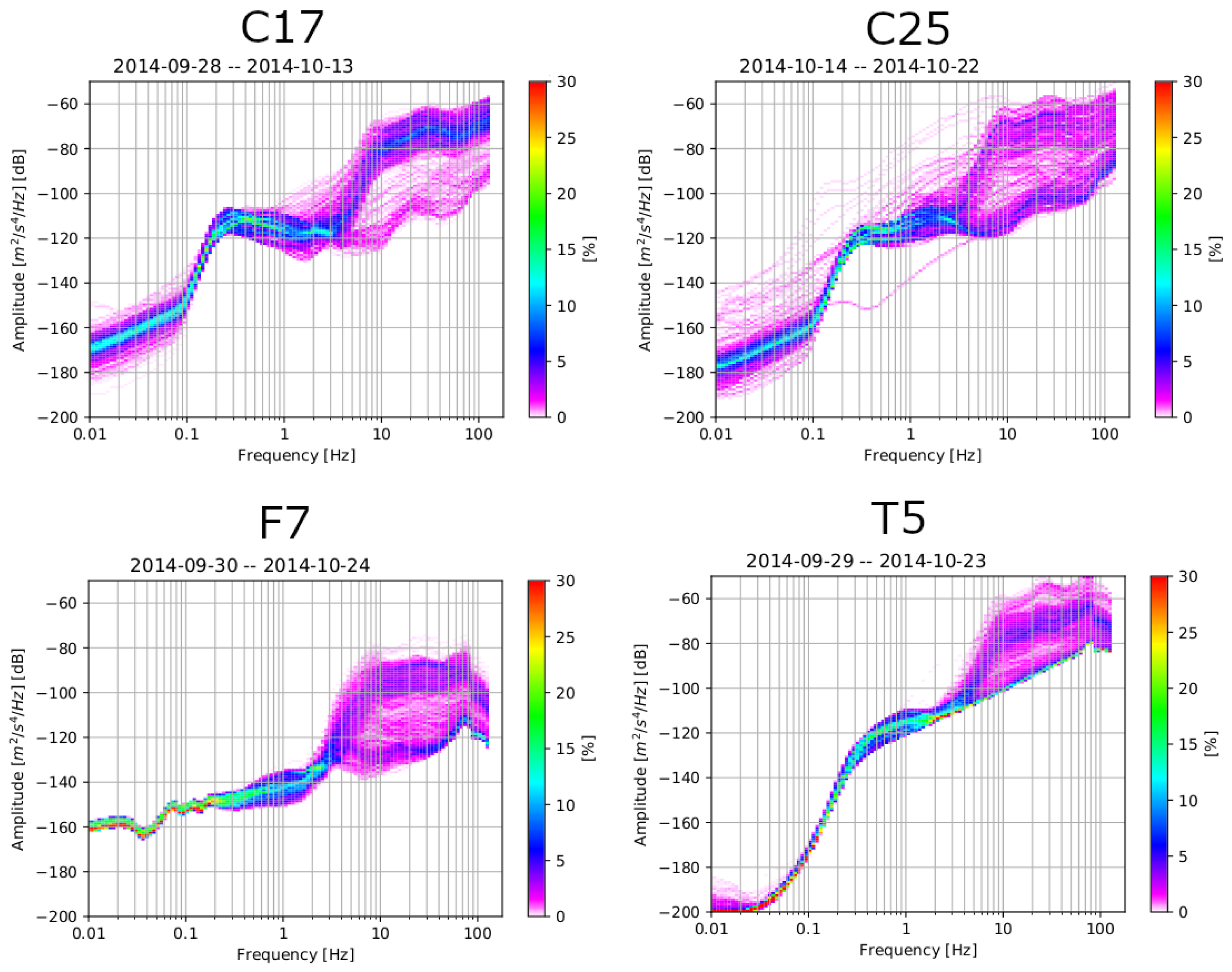
The PSD curves were estimated in terms of decibel at each frequency via direct Fourier transform introduced in [34]. PDFs were constructed at each frequency distribution bin by gathering PSDs in 1/8 octave of period intervals and 1 decibel of power intervals. We have shown 4 exemplary PDF plots in Figure 2. Each figure is for the vertical component of one station and during the whole time of recording. The PSD curves with higher probability distribution were interpreted as the ambient noise whereas the scattered PSD curves can be attributed to undesired signals [35]. The analysis indicates that the recorded energy is low at frequencies below ~0.1 Hz. Between 0.1 and 3 Hz, the curves reach a flat level showing low amplitude variations and a high probability level. At frequencies above 3 Hz, the variance between PSD curves increases significantly, which represent likely a result of random, local noises [33,36]. We used the PDF analysis in the junction with an inspection of the cross-correlation curves shown in the next section to limit the range of frequencies used in this study. This reduction of the frequency range speeds up the processing.
4.2. Cross-Correlation
Of the 43 available stations, we made sure to only correlate station data with identical instrumentation to avoid any potential phase bias, as we did not have access to the instrument response data. This left us with 200 possible station pairs. The signals recorded at each station were cut into time windows of 10 min with an overlap of 60 percent between successive windows. More complete explanations about the effects of overlapping time windows can be found in [37]. We did not explicitly remove earthquake signals which are expected to have only a minor effect on the obtained phase velocities [38]. However, we applied spectral whitening [39], to equalize spectral amplitudes and down-weight the effects of earthquake signals and monochromatic sources. The whitened 10-min segments were cross-correlated between station pairs and stacked. The cross-correlation traces show forward and backward propagating signals (causal/acausal) from opposing directions along the inter-station path, visible at positive and negative lag times in Figure 3. At inter-station distances greater 28 km, we did not observe any clear Rayleigh-wave signals whereas at distances below 5 km causal and acausal signals are not well-separated. This limitation is similar to the criteria of inter-station threshold recruited in the literature (see, e.g., in [36,39]) and resulted in 176 acceptable cross-correlations used in this study (Figure 3). The timedomain cross-correlations can be used to inspect the distribution of ambient-seismic-noise sources. Perfect symmetry between the cross-correlations at positive and negative lag times is an indicator of a homogeneous azimuthal noise-source distribution [28,29]. In theory, the waves moving in opposite directions should be identical between station pairs [40]. An asymmetric cross-correlation thus indicates a low signal-to-noise ratio.
We show 176 time-domain cross-correlations for four frequency bands 0.05–0.2 Hz, 0.2–0.4 Hz, 0.4–0.8 Hz, and 0.8–1.2 Hz in Figure 3 with regard to the inter-station distances on the vertical axis. We can discern the symmetry between positive and negative time lags in the frequency range of less than 0.8 Hz. The arrival of the Rayleigh wave signal cannot clearly be detected at higher frequencies (0.8–1.2 Hz). This loss means that the seismic noise sources are too weak and/or the random signals level is too high for a recording time of one month. Based on this analysis and the PDFs shown in the previous section, we limited our study to the frequency range between 0.05 and 1 Hz. This frequency range is in agreement with oceanic microseism utilized also in other seismic noise tomographic studies and typically generated by the non-linear interaction between the ocean and the solid earth (primary microseisms 0.07 Hz, secondary microseisms 0.14 Hz [18]). The amplitude differences between causal and acausal parts of the cross-correlations in Figure 4 are low, indicating a relatively homogeneous source distribution. This is supported by the more detailed comparison provided in Figure 4.
4.3. Amplitude Ratio
The amplitude ratios can be used to estimate the homogeneity of the noise-source distribution [41]. The amplitude ratio is defined as the maximum amplitude at the positive lag time of the cross-correlations over the maximum amplitude at negative lag time. The rose diagram in Figure 5 shows amplitude ratios of all station pairs in our array. This diagram is a proxy for the azimuthal distribution of noise sources. If two microseisms propagate along the inter-station path in opposite directions and with the same amplitude, the amplitude ratio will be one. If the ambient-noise energy coming from one direction is larger, we will observe a dominant direction in the rose diagram. A comparison of Figure 5A–D suggests that the noise–source distribution is more uniform at relatively high (Figure 5D) compared to relatively low (Figure 5A) frequencies. However, apart from some peaks in the rose diagrams, we find no clear preferential noise–source direction. In other words, the ambient noise sources are approximately equi-distributed within the studied frequency range which is another endorsement for the quality of time-domain cross-correlations.
4.4. Phase Velocity Determination
The cross-correlations can be used to obtain the empirical Green’s functions and were analyzed to gain information on the subsurface structure between the receiver pairs [42]. Most authors either picked group velocities by identifying the maximum in the envelope of surface-wave packets [43,44,45] or measured the phase velocity dispersion [46,47]. Fewer authors preferred utilizing the full waveform in their analysis [48]. In this study, we extracted phase velocities, because of the advantages in terms of accuracy, depth of investigation, and less contamination by interfering phases [42,49,50].
Several methods of phase-velocity measurements have been introduced such as the image transformation technique in the time-domain [51], the Frequency-wave number (F-K) method [52,53], multiple filter analysis [54], and Bessel function methods based on the theory of Aki [55] such as direct fitting in the frequency domain [56] or the herein applied zero-crossing fitting [38,47,49]. The intrinsic limitation of these methods is poor performance at low levels of signal-to-noise ratio. Plus, if the inter-station distance is too small, only few zero-crossings can be picked along the frequency axis, thus degrading the resolution of this method [56]. To mitigate these limitations, as explained above, we have only cross-correlated the station pairs distant by more than 5 km and also we checked the homogeneous distribution of sources in the data analysis (Figure 5D).
We used the previously computed cross-correlations and extract their zero crossings in the frequency domain (Figure 6). The zero crossings can be related to the phase velocity by comparison with the known zero crossings of a Bessel function [47,55]. We apply a smoothing filter to the cross-correlations which removes spurious zero crossings and thus stabilizes the obtained phase-velocity curves [49]. The phase-velocity picks from the 176 station-station cross-correlations were then taken manually. The picking procedure was performed in two iterations: after picking the phase-velocities for all station pairs in the first round, we calculated an average dispersion curve that was used to guide the manual picking in the second round. We applied several quality criteria: as explained above, we only accepted station pairs with an inter-station distance between 5 and 28 km. Because of their low signal-to-noise ratio, the French station data were not used. In addition, cross-correlations with large imaginary parts were discarded.
The average dispersion curve for 42 station pairs is shown in Figure 7. As expected from the noise analysis, only a few measurements at periods higher than 10 s could be taken. Therefore, we did not take any measurements above 10 s period into account in the depth inversion. To see the variations of phase velocities, the dispersion measurements were plotted at four periods (1.2, 2.5, 3.1, and 6 s) in Figure 8.
5. Inversion of Phase-Velocity Dispersion Curves
We made use of the dispersive nature of Rayleigh waves to obtain a 1D depthdependent shear-velocity profile. We used the average phase-velocity curve shown in Figure 7, thus neglecting any lateral variations of the subsurface structure. The dispersion curve can be inverted with linearized methods [57,58,59]. However, we preferred applying a Bayesian approach because of the highly nonlinear relation between phase velocity and subsurface structure and the subsequent non-uniqueness of the problem. We used the conditional neighborhood algorithm implemented in the Dinver software [60]. As in other Monte Carlo methods, we had to pre-define a range of priors for the pseudo-random sampling approach (Table 1). The range of statistical speculation and the role of prior information in this method are discussed in articles such as Scales and Tenorio [61] and Mosegaard and Tarantola [62]. Compared to other Monte Carlo approaches, the conditional neighborhood algorithm is more self-adaptive when searching through the parameter space. The search starts with a pre-defined number (ns0) of models distributed with a uniform probability in parameter space. The misfit function ( norm) is calculated for every model and the nr models with the lowest misfits are selected for the next iterations. This is iterated nt times, and at each iteration the selected lowest-misfit models are decomposed into ns/nr new models. The data misfit is given in relative units, normalized by the input data. In the conditional neighborhood algorithm, the dependency between parameters is taken into account at the beginning of the inversion by using a variable transformation [60].
The model is parameterized in terms of thickness, shear wave velocity (Vs), compressional wave velocity (Vp), and density () for each layer. Among them, Vs has the most important role and exercises the least influence on the dispersion curve. The Poisson’s ratio, which links Vs and Vp, was allowed to vary between 0.2 and 0.5 as indicated in Table 1, according to the value of Poisson’s ratio for geological materials [60]. Vp and Vs are free parameters of the inversion. The Poisson’s ratio is not a free parameter, but if a solution is generated with Vp and Vs such that the value of the Poisson’s ratio is outside of the allowed range, that solution is discarded. We chose the following model search parameters: ns0 = 50, nr = 50 and generated 10,000 models in total. We chose to use four layers whose prior ranges (Table 1) were defined based on the Preliminary Reference Earth Model (PREM) [63] and on several test runs in which we made sure that the search algorithm would generate a reasonably wide range of models centered around the measured data (Figure 9C). The obtained P-wave and S-wave velocity models are shown in Figure 9A,B, respectively. The black lines represent the average of the 5000 models with the lowest misfit and will be used for interpretation. The shown Vs profiles are more reliable, because of the higher sensitivity of Rayleigh waves to Vs compared to Vp.
6. Results and Discussion
We limit the discussion to the velocity models obtained from phase velocities up to a period of 10 s. This constraint allows investigating the subsurface structures down to ~15 km. In general, we consider our average Rayleigh-wave dispersion curve to be robust. Because Rayleigh waves are mostly sensitive to Vs, we are also confident that our Vs models are reasonably well constrained. Rayleigh waves are well known to be much less sensitive to Vp than Vs (see Figure 10), so our inferences are Vp and the Poisson’s ratio should be taken with care. We shall show, however, that the values we obtained are reasonable based on independent knowledge of those parameters. We also provide in Figure 9A,B a rough estimate of model uncertainty, defining as our confidence interval the range of values from three standard deviations below to three above the average. This definition of confidence is complicated near interfaces, where uncertainties in seismic velocity and interface depth are entangled with each other.
We first compare our average dispersion curve (Figure 9C) with results from ambientnoise tomography obtained in the south central Pacific (Figure 6 in [28]) and in the transform fault region of East Pacific Rise (Figure 4 in [29]). These two areas were selected as two of the rare examples where ambient-noise interferometry has been used to image the oceanic lithosphere. While our study areas are different, this qualitative comparison provided us with some insights from similar tectonic settings. In the average dispersion curve in Figure 7 and Figure 9C, we can identify an increasing trend of phase velocity up to a period of 20 s. This trend is similar to that found in the two other oceanic studies. Up to 16 s, both other regions have a phase velocity range of approximately 1.5–3.7 km/s while this range in our case is approximately 1–3.5 km/s. Lack of data in periods less than 2 s in Harmon et al. [28] probably account for the different minimum phase velocity.
Similar to our upper period bound of 10 s, Yao et al. [29] and Harmon et al. [28] mentioned that their phase velocity estimations for the fundamental mode of Rayleigh wave were subject to high uncertainty at periods greater than 8 s and 9 s, respectively. Nevertheless, longer recording time (200 days in [28] and over 1 year in [29]) enabled them to benefit from ambient noise data up to periods of 16 s and 30 s. A longer recording time will usually lead to a smoother distribution of incoming ambient-noise energy and suppresses errors in the dispersion-curve measurements [64].
The P-wave velocity in the crustal layer is expected to be lower than the velocity for olivine-rich gabbros, which is about 7 km/s [65] which we use to approximate the the Moho depth. Therefore, we infer an approximate crustal thickness of 7.2 km from Figure 9A. A similar conclusion can be drawn from the S-wave velocity model in Figure 9B, where the maximum expected crustal S-wave velocity is approx. 3.9 km/s [65]. This thickness is larger than the 4.2–5 km estimated from the P-wave velocity model in Momoh et al. [12] in the central part of the study area. The larger estimate of crustal thickness resulting from our approach could be due to the location of most used stations in the hanging wall compartment of the south facing active axial detachment fault (Figure 1). Both P-wave and S-wave velocity models represent almost linear and monotonic velocity to depth variations in Figure 9A,B.
As shown in Figure 9, the crustal range of S-wave velocities is approximately 1.1–3.9 km/s. It varies between 2.5 and 7 km/s for the P-wave velocity. We calculated the Vp/Vs ratio at different depths from our best Vp and Vs models (Figure 9). The comparison between the minimum and maximum values of S and P velocities gives a Vp/Vs ratio equal to 2.23 and 1.81, respectively (Figure 11). The ratio of P and S wave velocities provides an additional constraint on the the lithology [66] and is sensitive to the presence of fluids [67]. The high ratio of Vp/Vs = 2.23 at a shallower depth of the crust is indicative of high porosity and some amount of serpentinized peridotite. The minimum ratio of 1.81 is predicting lower porosity at deeper parts and is in agreement with Vp/Vs ratio of SWIR gabbroic rocks analyzed in Miller and Christensen [65]. Fast variations of P-wave and S-wave velocities at depths below 6.5–7.2 km and slow changes at depths >7.2 km can be another sign of permeability and porosity regime. This regime can affect the serpentinization process in the crust and upper mantle. The variable range of Vp/Vs in the crust and considerable serpentinization can be explained by the fracturing of the crust associated with detachment faults systems [68]. Another evidence of the fracturing of the crust was discovered in south dipping reflectors by Momoh et al. [12] which was interpreted as the damage zone. This zone is located within 2–2.8 km horizontally from the emergence of the active axial detachment fault system (deep regions on the map in Figure 1). The suggested serpentinization expressed in the velocity models is in agreement with seafloor sampling in non-corrugated oceanic core complexes collected from smooth (non-volcanic) seafloor [8].
We also compare our P-wave model with other models of ultramafic crusts. The Pwave velocity model of ultramafic crust at the Mid-Atlantic ridge at 23°N [69] is more linear and the observed velocity of the uppermost crust is higher than in our study, reaching the mantle faster. This higher range of velocity may be caused by gabbroic intrusions or fewer deformations of the exhumed, ultramafic crust in that region. The magma-poor rifted margins in Iberia-Newfoundland [70] and in western Iberia [71] also demonstrated a higher range of P-wave velocity in the upper ultramafic crust. Sedimentation and older ages of these margins likely explain why we observe this higher range of velocity.
An S-wave velocity higher than 3.9–4 km/s is typical for mantle rocks and our model is therefore indicating that unserpentinized and unfractured mantle is found at depths greater than 7 km. The average shear wave velocity between the base of the crust (defined by a 4 km/s Vs threshold), and the maximum depth of our model (15 km) is 4.2 km/s which is less than the global reference value of 4.5 km/s [72], that concerns old, off-axis oceanic lithosphere, but close to the 4.29 km/s of young oceanic lithosphere in the Pacific [29]. This relatively low value suggests that pristine and unfractured uppermost mantle may in fact be found deeper than 15 km below the hanging wall seafloor. This is consistent with results from a microseismicity study that shows earthquakes down to that depth in the investigated area (Jie et al., 2020 AGU abstract and paper soon to be submitted). The absence of a seismically well-defined and distinct Moho is consistent with reflectivity studies of Momoh et al. [12] in our study area. Moreover, other reflectivity studies predicted that more visible and recognizable Moho should be formed at faster spreading ridges, where mafic oceanic crust emplaced on the ultra-mafic mantle [73,74]. This prediction was also confirmed by another magma-poor ultra-slow spreading ridge by [75].
7. Conclusions and Outlook
1. We analyzed and cross-correlated ambient-noise recordings from 43 OBS stations. The symmetry of the cross-correlations in the time-domain and the amplitude ratio analysis showed that the noise source distribution is very homogeneous, despite the short operation time of the recorders.
2. The phase velocities extracted from the inter-station correlation functions ranged between 1 km/s to 3.5 km/s for periods between 1 s to 10 s and was in good agreement with other oceanic studies. Outside this period range, the low signal-to-noise ratio prohibited further analysis. Joint long time recording of ambient noise and earthquake data is proposed to cover also longer periods.
3. While the general P-wave velocity structure of our study is similar to previous works, we find a significantly thicker crust of ~7 km, averaged over the study region. At uppermost mantle depths, our results suggest an average shear velocity around 4.2 km/s which is less than the global average. This can be explained by the younger age of the seafloor in our area.
4. Our model suggests a very low S-wave velocity of around 1–1.5 km/s at shallow depths above 1 km in junction with a high Vp/Vs ratio of approx. 2.2. We infer that this may be due to the high porosity of the shallow, water-rich uppermost layer. The Vp/Vs ratio gradually decreases to ∼1.8 at a depth of 2.5 km. We propose that this transition reflects the decrease in porosity and assume a higher degree of serpentinization of the crustal material at shallow depths.
5. The ambient seismic noise method can be used as a complementary technique in geophysical studies of the oceanic lithosphere. The S-wave velocity model obtained provides new constraints to evaluate the velocity structure of the crust and uppermost mantle at a melt-poor portion of the ultra-slow spreading SWIR.
Author Contributions
Conceptualization, M.M.S., E.K., L.B., S.L. and M.C.; Formal analysis, M.M.S., E.K. and L.B.; Funding acquisition, S.L. and M.C.; Investigation, E.K., L.B., S.L. and M.C.; Methodology, M.M.S., E.K. and L.B.; Project administration, S.L. and M.C.; Resources, E.K., L.B., S.L. and M.C.; Software, M.M.S., E.K. and L.B.; Supervision, E.K., L.B., S.L. and M.C.; Validation, M.M.S., E.K., L.B., S.L. and M.C.; Visualization, M.M.S., E.K., L.B., S.L. and M.C.; Writing—original draft, M.M.S.; Writing—review and editing, M.M.S., E.K., L.B., S.L. and M.C. All authors have read and agreed to the published version of the manuscript.
Funding
Mohamadhasan Mohamadian Sarvandani is supported by a grant from ANR Ridge Factory 18-CE01-0002-01 and by Sorbonne Université. Emanuel Kästle has received funding from the German Science Foundation (SPP-2017, Project Ha 2403/21-1).
Institutional Review Board Statement
Not applicable for studies not involving humans.
Informed Consent Statement
Not applicable for studies not involving humans.
Data Availability Statement
Data are available on demand at https://data.ifremer.fr/SISMER.
Acknowledgments
The authors are grateful to the Flotte Océanographique Française (FOF) and an NSERC Ship Time grants that funded the SISMOSMOOTH cruise, and CNRS-INSU Tellus and ANR Rift2Ridge NT09-48546 for providing support for the cruise. Mohamadhasan Mohamadian Sarvandani is supported by a grant from ANR Ridge Factory 18-CE01-0002-01 and by Sorbonne Universite. Emanuel Kästle has received funding from the German Science Foundation (SPP-2017, Project Ha 2403/21-1).
Conflicts of Interest
The authors declare no conflict of interest.
References
- Sauter, D.; Cannat, M. The ultraslow spreading Southwest Indian ridge. Divers. Hydrotherm. Syst. Slow Spreading Ocean Ridges 2010, 88, 153–173. [Google Scholar]
- Cannat, M.; Rommevaux-Jestin, C.; Sauter, D.; Deplus, C.; Mendel, V. Formation of the axial relief at the very slow spreading Southwest Indian Ridge (49 to 69 E). J. Geophys. Res. Solid Earth 1999, 104, 22825–22843. [Google Scholar] [CrossRef]
- Sauter, D.; Carton, H.; Mendel, V.; Munschy, M.; Rommevaux-Jestin, C.; Schott, J.J.; Whitechurch, H. Ridge segmentation and the magnetic structure of the Southwest Indian Ridge (at 50 30′ E, 55 30′ E and 66 20′ E): Implications for magmatic processes at ultraslow-spreading centers. Geochem. Geophys. Geosyst. 2004, 5. [Google Scholar] [CrossRef]
- Carbotte, S.M.; Smith, D.K.; Cannat, M.; Klein, E.M. Tectonic and magmatic segmentation of the Global Ocean Ridge System: A synthesis of observations. Geol. Soc. Lond. Spec. Publ. 2016, 420, 249–295. [Google Scholar] [CrossRef]
- Dick, H.J.; Lin, J.; Schouten, H. An ultraslow-spreading class of ocean ridge. Nature 2003, 426, 405–412. [Google Scholar] [CrossRef]
- Momoh, E.; Cannat, M.; Leroy, S. Internal Structure of the Oceanic Lithosphere at a Melt-Starved Ultraslow-Spreading Mid-Ocean Ridge: Insights From 2-D Seismic Data. Geochem. Geophys. Geosyst. 2020, 21, e2019GC008540. [Google Scholar] [CrossRef]
- Cannat, M.; Sauter, D.; Mendel, V.; Ruellan, E.; Okino, K.; Escartin, J.; Combier, V.; Baala, M. Modes of seafloor generation at a melt-poor ultraslow-spreading ridge. Geology 2006, 34, 605–608. [Google Scholar] [CrossRef]
- Sauter, D.; Cannat, M.; Rouméjon, S.; Andreani, M.; Birot, D.; Bronner, A.; Brunelli, D.; Carlut, J.; Delacour, A.; Guyader, V.; et al. Continuous exhumation of mantle-derived rocks at the Southwest Indian Ridge for 11 million years. Nat. Geosci. 2013, 6, 314–320. [Google Scholar] [CrossRef] [Green Version]
- Zhao, M.; Qiu, X.; Li, J.; Sauter, D.; Ruan, A.; Chen, J.; Cannat, M.; Singh, S.; Zhang, J.; Wu, Z.; et al. Three-dimensional seismic structure of the Dragon Flag oceanic core complex at the ultraslow spreading Southwest Indian Ridge (49°39′ E). Geochem. Geophys. Geosyst. 2013, 14, 4544–4563. [Google Scholar] [CrossRef] [Green Version]
- Cannat, M.; Rommevaux-Jestin, C.; Fujimoto, H. Melt supply variations to a magma-poor ultra-slow spreading ridge (Southwest Indian Ridge 61° to 69°E). Geochem. Geophys. Geosyst. 2003, 4. [Google Scholar] [CrossRef]
- Tucholke, B.E.; Lin, J.; Kleinrock, M.C. Megamullions and mullion structure defining oceanic metamorphic core complexes on the Mid-Atlantic Ridge. J. Geophys. Res. Solid Earth 1998, 103, 9857–9866. [Google Scholar] [CrossRef] [Green Version]
- Momoh, E.; Cannat, M.; Watremez, L.; Leroy, S.; Singh, S.C. Quasi-3-D Seismic Reflection Imaging and Wide-Angle Velocity Structure of Nearly Amagmatic Oceanic Lithosphere at the Ultraslow-Spreading Southwest Indian Ridge. J. Geophys. Res. Solid Earth 2017, 122, 9511–9533. [Google Scholar] [CrossRef] [Green Version]
- Smith, D.K.; Cann, J.R.; Escartín, J. Widespread active detachment faulting and core complex formation near 13 N on the Mid-Atlantic Ridge. Nature 2006, 442, 440–443. [Google Scholar] [CrossRef] [PubMed]
- Standish, J.J.; Dick, H.J.; Michael, P.J.; Melson, W.G.; O’Hearn, T. MORB generation beneath the ultraslow spreading Southwest Indian Ridge (9–25 E): Major element chemistry and the importance of process versus source. Geochem. Geophys. Geosyst. 2008, 9. [Google Scholar] [CrossRef] [Green Version]
- Sauter, D.; Cannat, M.; Mendel, V. Magnetization of 0–26.5 Ma seafloor at the ultraslow spreading Southwest Indian Ridge, 61–67 E. Geochem. Geophys. Geosyst. 2008, 9. [Google Scholar] [CrossRef] [Green Version]
- Minshull, T.; Muller, M.; White, R. Crustal structure of the Southwest Indian Ridge at 66 E: Seismic constraints. Geophys. J. Int. 2006, 166, 135–147. [Google Scholar] [CrossRef] [Green Version]
- Chu, D.; Gordon, R.G. Evidence for motion between Nubia and Somalia along the Southwest Indian Ridge. Nature 1999, 398, 64–67. [Google Scholar] [CrossRef]
- Longuet-Higgins, M.S. A theory of the origin of microseisms. Philos. Trans. R. Soc. Lond. Ser. Math. Phys. Sci. 1950, 243, 1–35. [Google Scholar]
- Hasselmann, K. A statistical analysis of the generation of microseisms. Rev. Geophys. 1963, 1, 177–210. [Google Scholar] [CrossRef]
- Friedrich, A.; Krueger, F.; Klinge, K. Ocean-generated microseismic noise located with the Gräfenberg array. J. Seismol. 1998, 2, 47–64. [Google Scholar] [CrossRef]
- Campillo, M.; Paul, A. Long-range correlations in the diffuse seismic coda. Science 2003, 299, 547–549. [Google Scholar] [CrossRef] [Green Version]
- Shapiro, N.M.; Campillo, M. Emergence of broadband Rayleigh waves from correlations of the ambient seismic noise. Geophys. Res. Lett. 2004, 31. [Google Scholar] [CrossRef] [Green Version]
- Boschi, L.; Weemstra, C. Stationary-phase integrals in the cross correlation of ambient noise. Rev. Geophys. 2015, 53, 411–451. [Google Scholar] [CrossRef] [Green Version]
- Lin, F.C.; Ritzwoller, M.H.; Townend, J.; Bannister, S.; Savage, M.K. Ambient noise Rayleigh wave tomography of New Zealand. Geophys. J. Int. 2007, 170, 649–666. [Google Scholar] [CrossRef] [Green Version]
- Moschetti, M.; Ritzwoller, M.; Shapiro, N. Surface wave tomography of the western United States from ambient seismic noise: Rayleigh wave group velocity maps. Geochem. Geophys. Geosyst. 2007, 8. [Google Scholar] [CrossRef]
- Zheng, S.; Sun, X.; Song, X.; Yang, Y.; Ritzwoller, M.H. Surface wave tomography of China from ambient seismic noise correlation. Geochem. Geophys. Geosyst. 2008, 9. [Google Scholar] [CrossRef] [Green Version]
- Yang, Y.; Ritzwoller, M.H.; Levshin, A.L.; Shapiro, N.M. Ambient noise Rayleigh wave tomography across Europe. Geophys. J. Int. 2007, 168, 259–274. [Google Scholar] [CrossRef] [Green Version]
- Harmon, N.; Forsyth, D.; Webb, S. Using ambient seismic noise to determine short-period phase velocities and shallow shear velocities in young oceanic lithosphere. Bull. Seismol. Soc. Am. 2007, 97, 2009–2023. [Google Scholar] [CrossRef]
- Yao, H.; Gouedard, P.; Collins, J.A.; McGuire, J.J.; van der Hilst, R.D. Structure of young East Pacific Rise lithosphere from ambient noise correlation analysis of fundamental-and higher-mode Scholte-Rayleigh waves. C. R. Geosci. 2011, 343, 571–583. [Google Scholar] [CrossRef]
- Bohlen, T.; Kugler, S.; Klein, G.; Theilen, F. 1.5 D inversion of lateral variation of Scholte-wave dispersion. Geophysics 2004, 69, 330–344. [Google Scholar] [CrossRef]
- Leroy, S.; Cannat, M. MD 199/SISMO-SMOOTH Cruise, Marion Dufresne R/V. Fr. Oceanogr. Cruises 2014. [Google Scholar] [CrossRef]
- Leroy, S.; Cannat, M.; Momoh, E.I.; Singh, S.C.; Watremez, L.; Sauter, D.; Autin, J.; Louden, K.E.; Nedimovic, M.R.; Daniel, R.; et al. Seismic structure of an amagmatic section of the ultra-slow spreading South West Indian Ridge: The 2014 Sismosmooth cruise. AGUFM 2015, 2015, V21A–3027. [Google Scholar]
- McNamara, D.E.; Boaz, R. Seismic Noise Analysis System Using Power Spectral Density Probability Density Functions: A Stand-Alone Software Package. Available online: https://pubs.er.usgs.gov/publication/ofr20051438 (accessed on 4 June 2021).
- Cooley, J.W.; Tukey, J.W. An algorithm for the machine calculation of complex Fourier series. Math. Comput. 1965, 19, 297–301. [Google Scholar] [CrossRef]
- Agius, M.R.; D’Amico, S.; Galea, P.; Panzera, F. Performance evaluation of Wied Dalam (WDD) seismic station in Malta. J. Malta Chamb. Sci. 2014, 2, 72–80. [Google Scholar]
- Mordret, A.; Landès, M.; Shapiro, N.; Singh, S.; Roux, P.; Barkved, O. Near-surface study at the Valhall oil field from ambient noise surface wave tomography. Geophys. J. Int. 2013, 193, 1627–1643. [Google Scholar] [CrossRef]
- Seats, K.J.; Lawrence, J.F.; Prieto, G.A. Improved ambient noise correlation functions using Welch’ s method. Geophys. J. Int. 2012, 188, 513–523. [Google Scholar] [CrossRef] [Green Version]
- Ekström, G. Love and Rayleigh phase-velocity maps, 5–40 s, of the western and central USA from USArray data. Earth Planet. Sci. Lett. 2014, 402, 42–49. [Google Scholar] [CrossRef] [Green Version]
- Bensen, G.; Ritzwoller, M.; Barmin, M.; Levshin, A.; Lin, F.; Moschetti, M.; Shapiro, N.; Yang, Y. Processing seismic ambient noise data to obtain reliable broad-band surface wave dispersion measurements. Geophys. J. Int. 2007, 169, 1239–1260. [Google Scholar] [CrossRef] [Green Version]
- Li, H.; Bernardi, F.; Michelini, A. Surface wave dispersion measurements from ambient seismic noise analysis in Italy. Geophys. J. Int. 2010, 180, 1242–1252. [Google Scholar] [CrossRef] [Green Version]
- Liu, C.; Aslam, K.; Langston, C.A. Directionality of ambient noise in the Mississippi embayment. Geophys. J. Int. 2020, 223, 1100–1117. [Google Scholar] [CrossRef]
- Boschi, L.; Weemstra, C.; Verbeke, J.; Ekström, G.; Zunino, A.; Giardini, D. On measuring surface wave phase velocity from station–station cross-correlation of ambient signal. Geophys. J. Int. 2012, 192, 346–358. [Google Scholar] [CrossRef] [Green Version]
- Shapiro, N.M.; Campillo, M.; Stehly, L.; Ritzwoller, M.H. High-resolution surface-wave tomography from ambient seismic noise. Science 2005, 307, 1615–1618. [Google Scholar] [CrossRef] [PubMed] [Green Version]
- Stehly, L.; Campillo, M.; Shapiro, N. A study of the seismic noise from its long-range correlation properties. J. Geophys. Res. Solid Earth 2006, 111. [Google Scholar] [CrossRef]
- Stehly, L.; Fry, B.; Campillo, M.; Shapiro, N.; Guilbert, J.; Boschi, L.; Giardini, D. Tomography of the Alpine region from observations of seismic ambient noise. Geophys. J. Int. 2009, 178, 338–350. [Google Scholar] [CrossRef] [Green Version]
- Lin, F.C.; Moschetti, M.P.; Ritzwoller, M.H. Surface wave tomography of the western United States from ambient seismic noise: Rayleigh and Love wave phase velocity maps. Geophys. J. Int. 2008, 173, 281–298. [Google Scholar] [CrossRef] [Green Version]
- Ekström, G.; Abers, G.A.; Webb, S.C. Determination of surface-wave phase velocities across USArray from noise and Aki’s spectral formulation. Geophys. Res. Lett. 2009, 36. [Google Scholar] [CrossRef] [Green Version]
- Tromp, J.; Luo, Y.; Hanasoge, S.; Peter, D. Noise cross-correlation sensitivity kernels. Geophys. J. Int. 2010, 183, 791–819. [Google Scholar] [CrossRef] [Green Version]
- Kästle, E.D.; Soomro, R.; Weemstra, C.; Boschi, L.; Meier, T. Two-receiver measurements of phase velocity: Cross-validation of ambient-noise and earthquake-based observations. Geophys. J. Int. 2016, 207, 1493–1512. [Google Scholar] [CrossRef] [Green Version]
- Molinari, I.; Verbeke, J.; Boschi, L.; Kissling, E.; Morelli, A. Italian and Alpine three-dimensional crustal structure imaged by ambient-noise surface-wave dispersion. Geochem. Geophys. Geosyst. 2015, 16, 4405–4421. [Google Scholar] [CrossRef]
- Yao, H.; van Der Hilst, R.D.; De Hoop, M.V. Surface-wave array tomography in SE Tibet from ambient seismic noise and two-station analysis—I. Phase velocity maps. Geophys. J. Int. 2006, 166, 732–744. [Google Scholar] [CrossRef] [Green Version]
- Lacoss, R.T.; Kelly, E.J.; Toksöz, M.N. Estimation of seismic noise structure using arrays. Geophysics 1969, 34, 21–38. [Google Scholar] [CrossRef]
- Capon, J. High-resolution frequency-wavenumber spectrum analysis. Proc. IEEE 1969, 57, 1408–1418. [Google Scholar] [CrossRef] [Green Version]
- Herrmann, R.B. Computer programs in seismology: An evolving tool for instruction and research. Seismol. Res. Lett. 2013, 84, 1081–1088. [Google Scholar] [CrossRef]
- Aki, K. Space and time spectra of stationary stochastic waves, with special reference to microtremors. Bull. Earthq. Res. Inst. 1957, 35, 415–456. [Google Scholar]
- Menke, W.; Jin, G. Waveform fitting of cross spectra to determine phase velocity using Aki’s formula. Bull. Seismol. Soc. Am. 2015, 105, 1619–1627. [Google Scholar] [CrossRef]
- Herrmann, R. Computer Program in Seismology, Vol IV; St Louis University: St. Louis, MO, USA, 1994. [Google Scholar]
- Nolet, G. Linearized inversion of (teleseismic) data. In The Solution of the Inverse Problem in Geophysical Interpretation; Springer: Boston, MA, USA, 1981; pp. 9–37. [Google Scholar]
- Tarantola, A. Inversion of travel times and seismic waveforms. In Seismic Tomography; Springer: Dordrecht, The Netherlands, 1987; pp. 135–157. [Google Scholar]
- Wathelet, M. Array Recordings of Ambient Vibrations: Surface-Wave Inversion. Ph.D. Thesis, Liége University, Liège, Belgium, 2005. Volume 161. [Google Scholar]
- Scales, J.A.; Tenorio, L. Prior information and uncertainty in inverse problems. Geophysics 2001, 66, 389–397. [Google Scholar] [CrossRef] [Green Version]
- Mosegaard, K.; Tarantola, A. Monte Carlo sampling of solutions to inverse problems. J. Geophys. Res. Solid Earth 1995, 100, 12431–12447. [Google Scholar] [CrossRef]
- Dziewonski, A.M.; Anderson, D.L. Preliminary reference Earth model. Phys. Earth Planet. Inter. 1981, 25, 297–356. [Google Scholar] [CrossRef]
- Yao, H.; Beghein, C.; van der Hilst, R.D. Surface wave array tomography in SE Tibet from ambient seismic noise and two-station analysis–II. Crustal and upper-mantle structure. Geophys. J. Int. 2009, 173, 205–219. [Google Scholar] [CrossRef] [Green Version]
- Miller, D.J.; Christensen, N.I. Seismic velocities of lower crustal and upper mantle rocks from the slow-spreading Mid-Atlantic Ridge, south of the Kane Transform Zone (MARK). In Proceedings-Ocean Drilling Program Scientific Results; National Science Foundation: Alexandria, VA, USA, 1997; pp. 437–456. [Google Scholar]
- Kandilarov, A.; Mjelde, R.; Okino, K.; Murai, Y. Crustal structure of the ultra-slow spreading Knipovich Ridge, North Atlantic, along a presumed amagmatic portion of oceanic crustal formation. Mar. Geophys. Res. 2008, 29, 109–134. [Google Scholar] [CrossRef]
- Hamada, G. Reservoir fluids identification using Vp/Vs ratio? Oil Gas Sci. Technol. 2004, 59, 649–654. [Google Scholar] [CrossRef]
- Rouméjon, S.; Cannat, M.; Agrinier, P.; Godard, M.; Andreani, M. Serpentinization and fluid pathways in tectonically exhumed peridotites from the Southwest Indian Ridge (62–65E). J. Petrol. 2015, 56, 703–734. [Google Scholar] [CrossRef] [Green Version]
- Canales, J.P.; Collins, J.A.; Escartín, J.; Detrick, R.S. Seismic structure across the rift valley of the Mid-Atlantic Ridge at 23 20’(MARK area): Implications for crustal accretion processes at slow spreading ridges. J. Geophys. Res. Solid Earth 2000, 105, 28411–28425. [Google Scholar] [CrossRef]
- Minshull, T.A. Geophysical characterisation of the ocean–continent transition at magma-poor rifted margins. C. R. Geosci. 2009, 341, 382–393. [Google Scholar] [CrossRef] [Green Version]
- Davy, R.; Minshull, T.; Bayrakci, G.; Bull, J.; Klaeschen, D.; Papenberg, C.; Reston, T.J.; Sawyer, D.; Zelt, C. Continental hyperextension, mantle exhumation, and thin oceanic crust at the continent-ocean transition, West Iberia: New insights from wide-angle seismic. J. Geophys. Res. Solid Earth 2016, 121, 3177–3199. [Google Scholar] [CrossRef] [Green Version]
- Kennett, B.L.; Engdahl, E.; Buland, R. Constraints on seismic velocities in the Earth from traveltimes. Geophys. J. Int. 1995, 122, 108–124. [Google Scholar] [CrossRef]
- Aghaei, O.; Nedimović, M.R.; Carton, H.; Carbotte, S.M.; Canales, J.P.; Mutter, J.C. Crustal thickness and Moho character of the fast-spreading East Pacific Rise from 9°42′ N to 9°57′ N from poststack-migrated 3-D MCS data. Geochem. Geophys. Geosyst. 2014, 15, 634–657. [Google Scholar] [CrossRef] [Green Version]
- Boulahanis, B.; Carbotte, S.M.; Huybers, P.J.; Nedimović, M.R.; Aghaei, O.; Canales, J.P.; Langmuir, C.H. Do sea level variations influence mid-ocean ridge magma supply? A test using crustal thickness and bathymetry data from the East Pacific Rise. Earth Planet. Sci. Lett. 2020, 535, 116121. [Google Scholar] [CrossRef]
- Grevemeyer, I.; Hayman, N.W.; Peirce, C.; Schwardt, M.; Van Avendonk, H.J.; Dannowski, A.; Papenberg, C. Episodic magmatism and serpentinized mantle exhumation at an ultraslow-spreading centre. Nat. Geosci. 2018, 11, 444–448. [Google Scholar] [CrossRef]
Figure 1.
(A) Free-air gravity anomalies over Southwest Indian Ridge (SWIR). The thin black line shows SWIR axis. Variation of fracture zones orientation represents the variation of spreading direction with time [17]. The blue rectangle marks our study area. (B) Bathymetry map of the study area. The locations of ocean bottom seismometers are shown by reverse triangles. The final stations used for inversion are indicated by black color and the removed stations based on data analysis are shown by gray color. Most of the stations have been placed on smooth seafloor. The red thick line is the axis and the purple line is indicating the emergence of the axial detachment fault system. The breakaway of the active fault is located at the top of the northern axial valley and suggested breakaways of inactive faults are seen in the southern Antarctic plate.

Figure 2.
Initial analysis of noise data: every individual curve gives the power spectral density (PSD). Color bars display the probability of distribution of seismic power spectral density at different frequencies. Every plot represents the vertical component of one station (station ID at the top) during the entire recording time. Both high amplitudes and low signal variability can be observed mostly between 0.1 and 3 Hz.

Figure 3.
Cross-correlation in time domain for all the station pairs with inter-station distance between 5 and 28 km and for four frequency bands (A) 0.05–0.2 Hz, (B) 0.2–0.4 Hz, (C) 0.4–0.8 Hz, and (D) 0.8–1.2 Hz. The symmetry in positive and negative lags show the ambient-noise sources were homogeneously distributed. This symmetry is best observable for frequencies less than 0.8 Hz.

Figure 4.
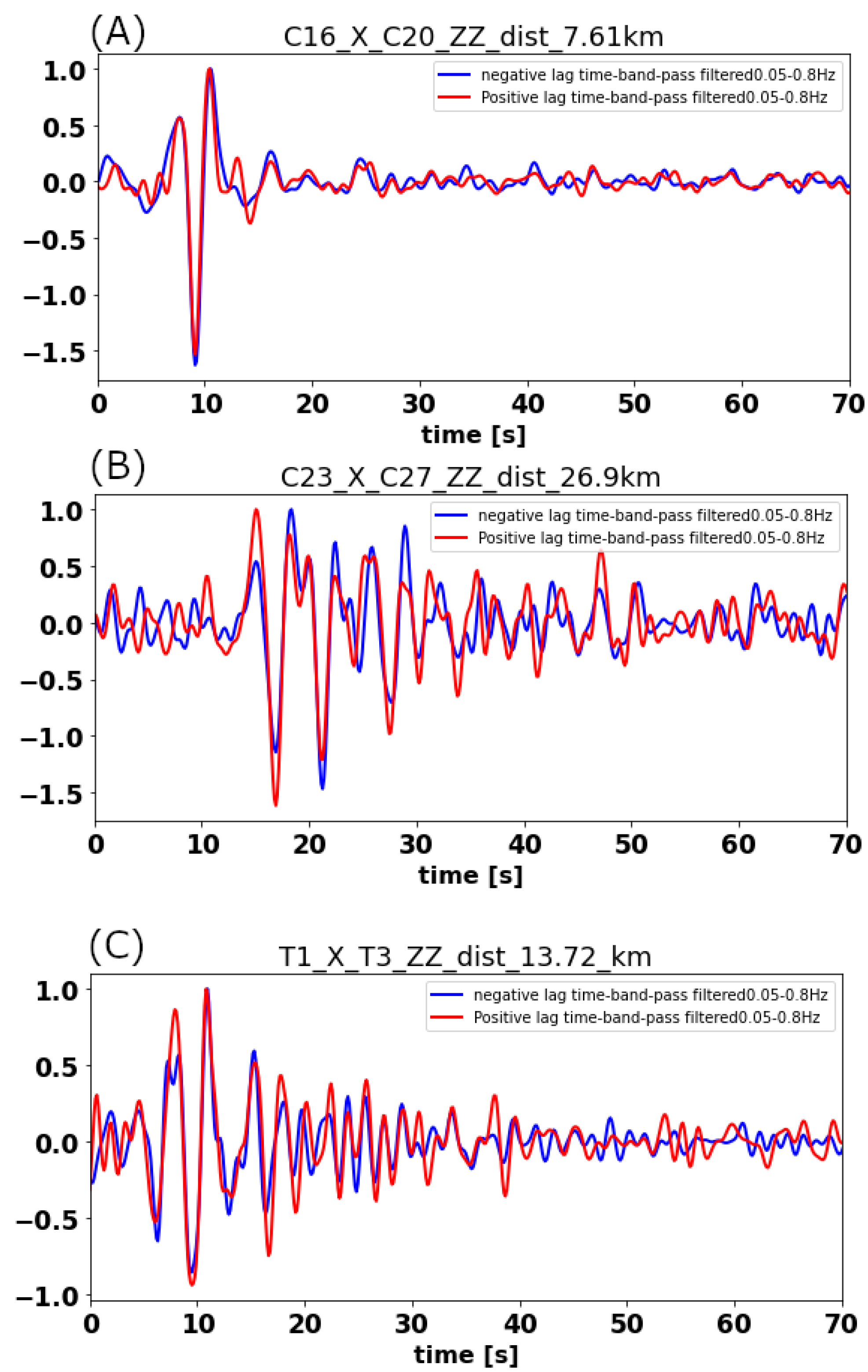
Comparison between the positive and negative lag time signals of station pairs (A) C16–C20, (B) C23–C27, and (C) T1–T3. The name of station pair, type of receiver (zz = vertical) and the inter-station distance in km is given at the top of every panel. Red lines show the positive lag time signal, flipped onto the negative time axis. The selected range of frequency is 0.05–0.8 Hz. The good overlap between positive and negative lag time signals confirms the symmetry in time domain cross-correlation and is taken as indication of the spatial homogeneity of source distribution.
Figure 4.
Comparison between the positive and negative lag time signals of station pairs (A) C16–C20, (B) C23–C27, and (C) T1–T3. The name of station pair, type of receiver (zz = vertical) and the inter-station distance in km is given at the top of every panel. Red lines show the positive lag time signal, flipped onto the negative time axis. The selected range of frequency is 0.05–0.8 Hz. The good overlap between positive and negative lag time signals confirms the symmetry in time domain cross-correlation and is taken as indication of the spatial homogeneity of source distribution.

Figure 5.
Rose diagrams of amplitude ratios for frequency bands: (A) 0.05–0.2 Hz, (B) 0.2–0.4 Hz, (C) 0.4–0.8 Hz, and (D) 0.05–0.8 Hz. The rose diagrams serve as proxy for the azimuthal distribution of noise sources.
Figure 5.
Rose diagrams of amplitude ratios for frequency bands: (A) 0.05–0.2 Hz, (B) 0.2–0.4 Hz, (C) 0.4–0.8 Hz, and (D) 0.05–0.8 Hz. The rose diagrams serve as proxy for the azimuthal distribution of noise sources.

Figure 6.
(A) Real part of the cross-correlation of station pair C23–C27 with an inter-station distance of 26.9 km in the frequency domain. (B) Cross-correlation of station pair C23–C27 in the time domain. (C) Real part of the cross-correlation of station pair T1–T3 with an inter-station distance of 13.72 km in the frequency domain. (D) Cross-correlation of station pair T1–T3 in the time domain. Smoothing (green line) helps to reduce the effect of spurious zero crossings [49]. The smoothed cross-correlations in the time domain (green and blue) are symmetric around time zero since the imaginary part of the frequency domain cross-correlation was set to zero prior to the inverse Fourier transform. According to the data analysis, the maximum range of frequency set to 1 Hz.

Figure 7.
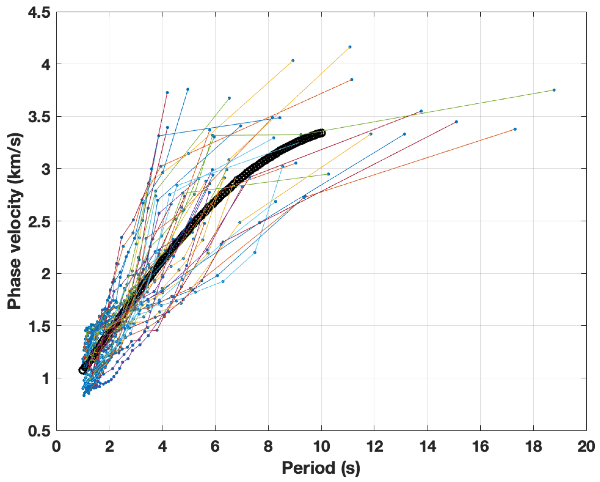
The picked phase velocity of every station pair is shown as colored lines. Blue circles are all the picked phase velocities. The thick black curve gives the average dispersion curve of all the picked data up to a maximum of 10 s.
Figure 7.
The picked phase velocity of every station pair is shown as colored lines. Blue circles are all the picked phase velocities. The thick black curve gives the average dispersion curve of all the picked data up to a maximum of 10 s.

Figure 8.
Phase velocity variations are indicated in (A) period 1.2 s, (B) period 2.1 s, (C) period 3.1 s, and (D) period 6 s. Reverse triangles indicate the location of the stations used in the final analysis. An increasing trend of the measured phase velocity from shorter to longer periods is observable.

Figure 9.
(A) 5000 lowest misfit P-wave velocity models, and (B) corresponding S-wave velocity model, with color denoting misfit value, as indicated by the color bars. The black solid lines denote the Vp and Vs averages of all shown models. Dashed lines identify our selected confidence interval, which we define as three standard deviations above and below the average, at each depth. Bulges in the dashed lines around discontinuities are inevitable artifacts of combining uncertainty in seismic velocity and discontinuity depth. (C) Rayleigh phase-velocity data corresponding to the models in (A,B). The black curve in panel (C) identifies the picked values of phase velocity.

Figure 10.
Sensitivity kernels relating Rayleigh-wave phase velocity estimates to Vs (left) and Vp (right) at depth. Note the difference in horizontal scale between the left and right panels: sensitivity of Rayleigh waves to Vp is one-order-of-magnitude smaller than their sensitivity to Vs, as expected. The reference assumed for the computation of the kernels is our final Vp, Vs profile (solid black lines in Figure 9A,B). Kernels were calculated via Keurfon Luu’s “disba” Python package.

Figure 11.
Vp/Vs ratio (thick black line), obtained from the final Vp and Vs models (black curves in Figure 9A,B), as a function of depth. Dashed lines identify the confidence interval, defined as in Figure 10. Full distribution of sampled models with the lowest misfit are shown in color.


Table 1.
Parameterization for inversion.
| Layer | Vs(m/s) | Depth (m) | Vp(m/s) | Poisson’s Ratio | Density |
|---|---|---|---|---|---|
| V0 | 200 to 1500 | 200 to 5000 | 300 to 3500 | 0.2 to 0.5 | 2.4 |
| V1 | 1500 to 2800 | 1000 to 8000 | 2000 to 6500 | 0.2 to 0.5 | 2.6 |
| V2 | 2600 to 3900 | 2000 to 12,000 | 3500 to 9000 | 0.2 to 0.5 | 2.9 |
| V3 | 4200 to 5500 | - | 4000 to 12,000 | 0.2 to 0.5 | 3.4 |
Publisher’s Note: MDPI stays neutral with regard to jurisdictional claims in published maps and institutional affiliations. |
© 2021 by the authors. Licensee MDPI, Basel, Switzerland. This article is an open access article distributed under the terms and conditions of the Creative Commons Attribution (CC BY) license (https://creativecommons.org/licenses/by/4.0/).
Share and Cite
MDPI and ACS Style
Mohamadian Sarvandani, M.; Kästle, E.; Boschi, L.; Leroy, S.; Cannat, M. Seismic Ambient Noise Imaging of a Quasi-Amagmatic Ultra-Slow Spreading Ridge. Remote Sens. 2021, 13, 2811. https://0-doi-org.brum.beds.ac.uk/10.3390/rs13142811
AMA Style
Mohamadian Sarvandani M, Kästle E, Boschi L, Leroy S, Cannat M. Seismic Ambient Noise Imaging of a Quasi-Amagmatic Ultra-Slow Spreading Ridge. Remote Sensing. 2021; 13(14):2811. https://0-doi-org.brum.beds.ac.uk/10.3390/rs13142811
Chicago/Turabian StyleMohamadian Sarvandani, Mohamadhasan, Emanuel Kästle, Lapo Boschi, Sylvie Leroy, and Mathilde Cannat. 2021. "Seismic Ambient Noise Imaging of a Quasi-Amagmatic Ultra-Slow Spreading Ridge" Remote Sensing 13, no. 14: 2811. https://0-doi-org.brum.beds.ac.uk/10.3390/rs13142811
Note that from the first issue of 2016, this journal uses article numbers instead of page numbers. See further details here.