Exploring the Impacts and Temporal Variations of Different Building Roof Types on Surface Urban Heat Island

Abstract

This study examined the impact of different types of building roofs on urban heat islands. This was carried out using building roof data from remotely sensed Landsat 8 Operational Land Imager (OLI) and Thermal Infrared Sensor (TIRS) imagery. The roofs captured included white surface, blue steel, dark metal, other dark material, and residential roofs; these roofs were compared alongside three natural land covers (i.e., forest trees, grassland, and water). We also collected ancillary data including building height, building density, and distance to the city center. The impacts of various building roofs on land surface temperature (LST) were examined by analyzing their correlation and temporal variations. First, we examined the LST characteristics of five building roof types and three natural land covers using boxplots and variance analysis with post hoc tests. Then, multivariate regression analysis was used to explore the impact of building roofs on LST. There were three key findings in the results. First, the mean LSTs for five different building roofs statistically differed from each other; these differences were more significant during the hot season than the cool season. Second, the impact of the five types of roofs on LSTs varied considerably from each other. Lastly, the contribution of the five roof types to LST variance was more substantial during the cool season. These findings unveil specific urban heat retention drivers, in which different types of building roofs are one such driver. The outcomes from this research may help policymakers develop more effective strategies to address the surface urban heat island phenomenon and its related health concerns.

1. Introduction

In recent decades, several developed and developing countries have undergone urbanization and industrialization. This rapid development in urban areas has led to an environmental issue known as the surface urban heat island (SUHI), which affects more than half of the urban population [1,2,3,4]. SUHI is a phenomenon in which urban areas have higher surface temperatures than their suburban/rural counterparts [5,6,7,8]. Land surface temperature (LST) is a significant parameter used to explore the exchange of surface matter, surface energy balance, and surface physico-chemical processes. Thus, it is one of the most essential sources used to characterize SUHIs [9]. LST represents the energy exchange between the land and atmosphere, an important geophysical parameter in ground–air systems [10].

Many researchers have employed a general land cover class known as the impervious surface area (ISA) for SUHI analysis. Typically, information on the ISA information is extracted from remotely sensed images and viewed as a pure land cover class in previous studies. The ISA information used in SUHI analysis includes the ISA percentage in an image pixel [11], ISA indices [12], and the ISA class [13]. The major limitation of existing studies is that the ISA is considered a pure class for analysis; here, the impact of finer ISAs on LST and their temporal variation have not yet been systematically analyzed. The ISA contains several sub-classes, including white surface, blue steel, dark metal, other dark material, and residential roofs [14,15]. Each sub-class is characterized by different physical properties and are the fundamental elements responsible for changes in surface energy flux [16,17]. The reflectance of each finer ISA class changes with the difference in the material or the building surface. For example, the reflectivity of other dark material and residential roofs is usually lower than metal and galvanized steel roofs. Additionally, the reflectivity of weathered roofs is not as high as that of newly built roofs [18]. As such, representation of the whole ISA with only one or two classes (e.g., high albedo–low albedo, bright ISA–dark ISA, built-up area, and urban area) may be insufficient to understand the impact of finer ISAs on the LST [19]. Similarly, different times or seasons also affect the retrieval temperature of the building roof. For example, the surface of the roof absorbs a large amount of solar radiation during the day; as such, its surface temperature is high. However, at night, without solar radiation, the roof is able to rapidly cool down and maintain a lower temperature. Moreover, the roof surface can freely exchange long-wave radiation when remote sensing images are cloud-free. The external shape of the building and the color of the roof coating also affect temperature [18].

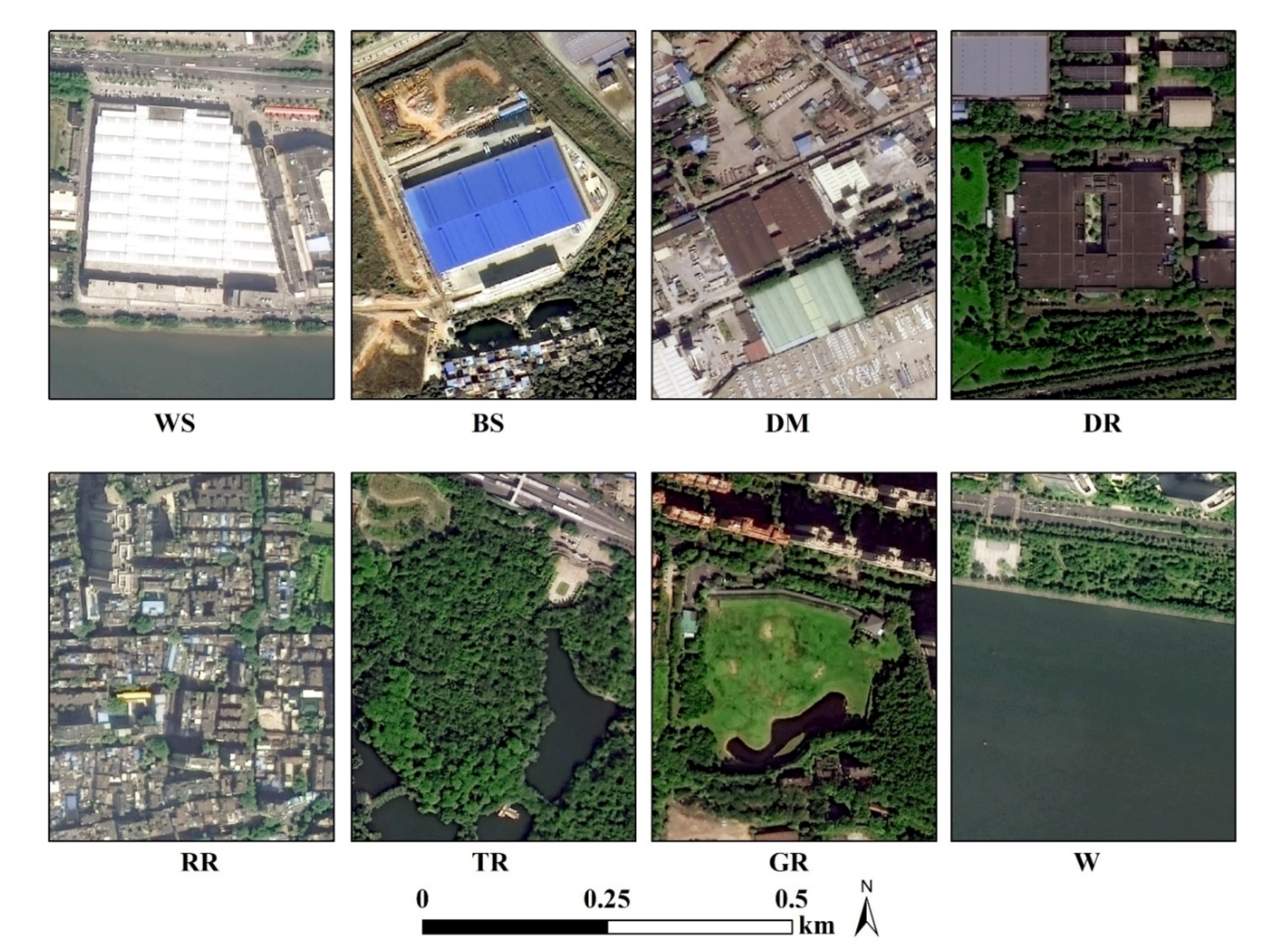
In this context, this study aims to examine two key aspects: (1) the distinct impacts of different building roofs (finer ISA classes) on LST, and (2) whether these particular impacts unveil temporal variations. We classified ISAs into five types of building roofs: white surface (WS), blue steel (BS), dark metal (DM), other dark material (DR), and residential roofs (RR). We also included three natural land cover types: forest, grass, and water. Multivariate regression analysis with dummy variables of ISA classes and natural land covers was used to explore the impacts of finer ISA classes on the LST. The remainder of this paper was structured into four sections. 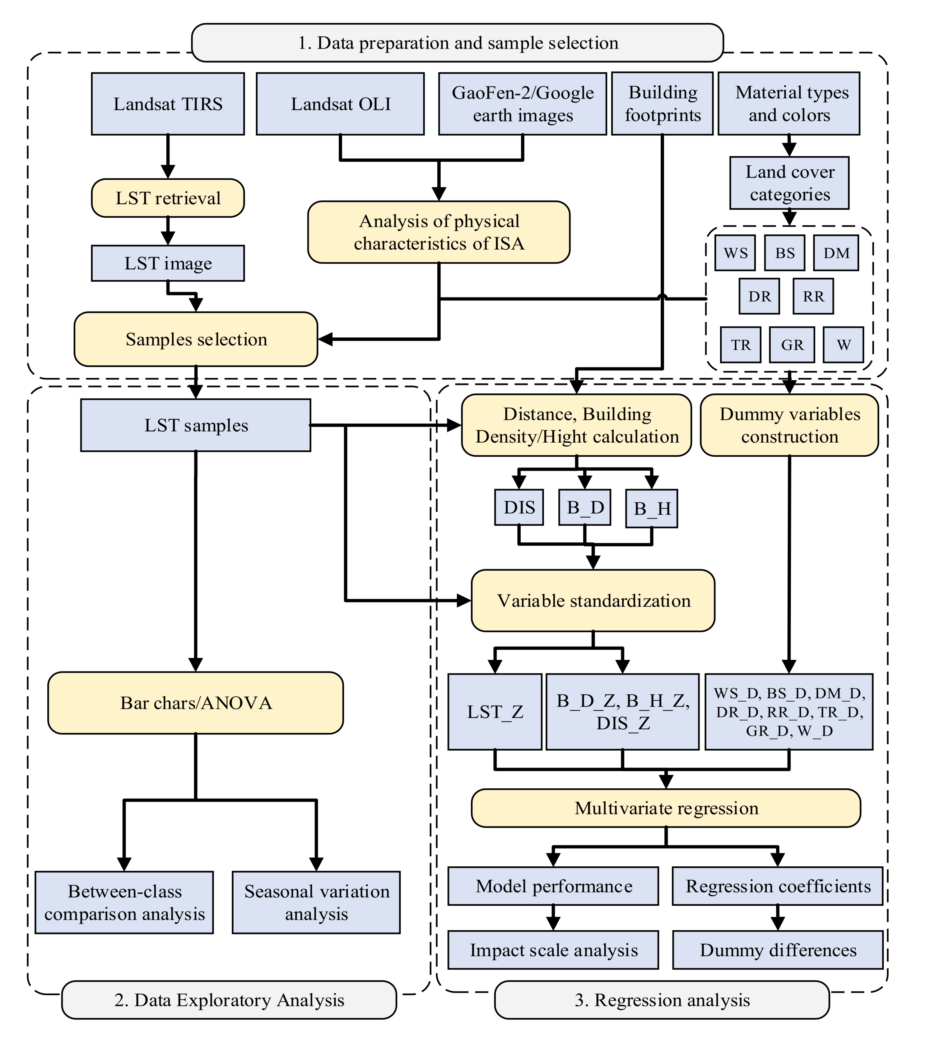Section 2 describes the methodology, including the study area, data source, data pre-processing method, and regression analysis. Section 3 presents the results from analyzing four years of hot and cool seasons. Section 4 discusses the results, and Section 5 concludes the study.

2. Materials and Process

2.1. Study Area

Guangzhou and Foshan are cities in Guangdong Province, China (22°56′N to 23°93′N and 112°38′E to 114°05′E), both of which were selected as the study area (Figure 1). They are located in southern China and the northern part of the Pearl River Delta, spanning a combined area of 11,231 km². Guangzhou and Foshan experience a humid subtropical climate affected by the East Asian monsoon. Summers are hot and humid, while winters are warm and less humid. Guangzhou and Foshan are core regions of the Guangdong–Hong Kong–Macao Greater Bay Area (GBA), with the highest population density in Guangdong Province and being the national center of South China. By the end of 2018, the population of these two cities exceeded 22 million.

2.2. Data Sources

Imagery from the Landsat 8 Operational Land Imager (OLI) and Thermal Infrared Sensor (TIRS) with a spatial resolution of 30 m were used as the data sources in this study (Figure 2). The data were recorded during the hot and cool seasons; the specific dates and corresponding temperature ranges are listed in

Table 1. Selected dates of Landsat 8 imageries and their associated daily temperature ranges.

	Cool Season		Hot Season
Year	Date	Temperature (°C)	Date	Temperature (°C)
2014	16 January 2014	4–19	9 August 2013	25–34
2016	7 February 2016	5–17	18 September 2016	25–33
2018	12 February 2018	7–18	22 July 2018	26–34
2020	18 February 2020	7-19	27 September 2019	23–32

[20]. No cloud-free images were available during the hot seasons in 2014 and 2020. Thus, images recorded during the hot season from previous years (i.e., 2013H and 2019H) were used as substitutes for 2014H and 2020H (Table 1). High spatial resolution imagery acquired from Google Earth historical images (for 2014, 2016, 2018, and 2020) and GaoFen-2 imagery (for 2016 and 2019) were used to assist in sample selection. Building outlines containing building height information were used to obtain data on the building density and determine the average building height. The building outline data were supplied from a geographic information system (GIS) company (ZhongKe Tuxin Co., Ltd. Location: Suzhou Science and Technology City Chinese Academy of Sciences Geographic Information and Cultural Science and Technology Industry Base; http://www.tuxingis.com//index.html, accessed on 12 November 2020). As these building outlines were only available for urban areas, there were no samples taken from suburban or rural areas. All remotely sensed data were pre-processed with calibration and atmospheric correction, and all data were re-projected to the Universal Transverse Mercator (UTM) projection in zone 49N.

3. Method

This section is made up of three parts. Section 3.1 discusses the data preparation, including the definition of the finer ISA class, LST retrieval, and sample selection. Section 3.2 focuses on data variance analysis using charts and analysis of variance (ANOVA). Finally, Section 3.3 discusses the process of establishing the multivariate linear regression including variables such as building density, average building height, distance to city center, dummy variable construction, and the standardization of variables. A flowchart of the research design is shown in Figure 3.

3.1. Data Preparation and Sample Selection

3.1.1. Definitions of Types of Building Roofs and Natural Land Covers

Following careful investigations using high spatial resolution imagery and field trip surveys, we subdivided the land surfaces of the study area into five ISA classes on the basis of different types of building roofs and three natural land cover classes (Figure 4). First, five ISA classes, namely, WS, BS, DM, DR, and RR, were divided on the basis of their color and material properties. The WS consisted of white building roofs made of polished white galvanized steel, while the BS included a steel panel painted in blue. DM refers to a rusty steel panel that is brown or dark in color, while the DR contains all dark-colored roofs that usually expand over large areas. RR represents residential roofs that consist of loosely distributed residential buildings within a neighborhood. Due to the limited spatial resolution of data sourced from Landsat imagery, the RR reflectance may be affected by shadows and vegetation. As such, the RR was assigned as an independent class for two reasons: (1) its land-use type is residential, where each patch has a small area, and the building heights are generally low, making sample selection difficult, and (2) it is a common land-use type scattered across urban areas with a significant impact on the LST distribution. Types of vegetation cover were classified as tree (TR) or grass (GR) categories; agricultural land was assigned to the latter class. The water (W) class, which contains surface waters such as lakes and rivers, was also used, while soil was excluded because its heat property is affected by moisture.

To elucidate the difference between classes, we collected data on the physical characteristics from previous studies, including the thermal conductivity coefficient and albedo value (

Table 2. Thermal conductivity coefficients, color, and albedo of different land cover classes.

Land Cover Types	Thermal Conductivity Coefficient (W/m K)	Color	Albedo
WS	35–70	White	0.75
BS	10–60	Blue	0.1–0.75
DM	10–60	Black, drown	<=0.1
DR	0.75	Black, deep gray	<=0.1
RR	0.40–0.70	Black, deep gray	<0.1
GR	-	Green	0.18–0.25
TR	-	Green, deep green	0.03–0.3
W	0.606	-	0.02–0.05

) [21,22,23,24,25,26,27]. The thermal conductivity coefficient illustrates that metal-like materials, such as WS, BS, and DM, have the highest values. This indicates that these materials absorb heat more rapidly and are thus quick to heat up. In other finer ISA classes, such as DR and RR, the thermal conductivity coefficients were found to be much lower than the WS, BS, and DM. The thermal conductivity coefficient of W was similar to that of RR (0.606). Albedo was an additional factor recognized to affect LST and was related to color; a white color has the highest albedo, while a black color has the lowest. A higher albedo value implies that more energy is reflected, and less energy is absorbed by the materials. As a result, the temperature of a high-albedo material is generally lower than a low-albedo material. Table 2 shows that the albedo of WS was the highest, whereas the albedo values of DM, DR, and RR were close to 0.1. The albedo of BS albedo was between 0.1 and 0.75, in terms of the color gradation. Generally, the albedo of GR was higher than TR, as its lowest albedo was much larger than TR; however, TR had the highest albedo according to the different types of trees. The albedo of W was almost zero, indicating negligible reflectance in this class.

3.1.2. Land Surface Temperature Retrieval

The original LST was retrieved using a method of atmospheric correction, the radiative transfer equation, in the single-channel algorithm with Band 11 in Landsat 8 TIRS [28,29,30]. This study adopted the calculation method developed by Jimenez-Munoz [30], which describes the detailed calculation process.

3.1.3. Sample Selection and LST Extraction

Samples of different building roofs and natural land covers (one pixel: 30 m × 30 m) were collected from the LST imagery, with the assistance of high spatial resolution images. Then, we used three windows to present the high spatial resolution, LST, and Landsat imagery using ENVI, the commercial software (https://www.ittvis.com/envi/, accessed on 1 November 2018). These three windows were geographically linked such that when moving the focus on the high spatial resolution image window, the corresponding location will change accordingly in the other two windows. We then investigated the entire study area in the high spatial resolution image window and labeled the building roofs that covered more than 9 pixels in the LST imagery. The pixel of the LST image, which was in the center of the building roof, was selected as the sample (see Figure 5, rectangle outlined by green dashed line). Finally, the value of the selected pixel in the LST image was extracted and stored in a table for statistical analysis. The selection of the natural land cover type used the same method as the building roof sample selection. The hot- and cool-season readings for different years were taken from the same samples in the LST imagery; the number of samples for each class is listed in

Table 3. The number of samples for each building roof and natural land cover class.

Types	2014	2016	2018	2020
WS	113	107	96	101
BS	97	103	91	100
DM	61	94	97	90
DR	80	98	109	109
RR	100	109	122	99
TR	100	108	164	101
GR	91	108	164	106
W	110	106	104	104
Total	752	833	947	810

.

3.2. Data Exploratory Analysis

3.2.1. Between-Class Comparison Analysis

Bar charts were used to illustrate the mean LST for each class; a comparison between classes may be easily interpreted by comparing the height of each class in the bar chart. In addition, one-way ANOVA was applied to compare the LST means to test whether there were any statistically significant differences between the different land cover types. In this study, ANOVA combined with a post hoc test was applied to LST data for each season of every year to determine whether there was a statistically significant difference between different land cover types during the hot and cool seasons.

3.2.2. Seasonal Variation Analysis

Seasonal variation was analyzed by comparing the variance of the mean LST in hot and cool seasons. The bar chart describes different values using the height of the bar and enabled an easy comparison of the differences between the two values. Thus, the mean LST of each class was assembled in a bar chart to illustrate the variation between seasons and years.

3.3. Regression Analysis

3.3.1. Determining the Building Density, Average Building Height, and Distance to City Center

The outline of a building along with building height information were utilized to calculate the building density (B_D) and average building height (B_H) in each sample. This information was downloaded from the open street map (OSM). Building density was computed using the total area of the building within a sample (pixel) divided by the total area of the sample (1 pixel, 30 m × 30 m = 900 m²). The determination of B_D and B_H were based on Equations (1) and (2), respectively:

$$B\_D={\displaystyle \sum _{i=1}^N{B}_{i,a}}/A_s,$$

(1)

$$B\_H={\displaystyle \sum _{i=1}^N(B_{i,h}\times B_{i,a}/A_s)}/N,$$

(2)

where B_i,a and A_s are the area of building, i, within a sample and the total area of the sample, respectively; B_i,h is the height of building i; and N is the number of buildings in a sample.

We also calculated the distance between the sample and city center. As this study was based on two cities, we calculated the distances between samples and city centers using the Euclidean distance; the shortest distance to the city center was used for the analysis. The distance was calculated using Equation (3):

$$DIS=\sqrt{{(x_1-x_2)}^2+{(y_1-y_2)}^2},$$

(3)

where DIS is the distance between the sample and city center, x₁ and y₁ are the sample coordinates, and x₂ and y₂ are the city center coordinates.

3.3.2. Dummy Variables Construction

Dummy variables were applied for attributes with more than one distinct category in regression analysis [31]. These variables operate as switches, such that they filter non-related cases in a regression model. Dummy variables were limited to two specific values: 1 or 0. Typically, 1 indicates the presence of a qualitative attribute, while 0 indicates otherwise. In detail, an dummy variable was created to represent an attribute with two or more distinct classes [31]. For each class, all missing values were recoded to “0” to minimize the impact of missing values on model results. The dummy variables were created to indicate whether “0” is a missing value or is the average (good) performance [32]. For example, the regression equation obtained with quantitative variables using the least square method is often difficult to fit; therefore, it is challenging to accurately reflect the internal relationship between elements in the city. Thus, dummy variables were introduced to filter irrelevant factors in the model, which may enhance model robustness [33,34,35]. The building roof types (WS, BS, DM, DR, and RR) and natural land covers (TR, GR, and W) were recoded as dummy variables (i.e., WS_D, BS_D, DM_D, DR_D, RR_D, TR_D, GR_D, and W_D, respectively). For example, if a sample belonged to WS, a value of 1 was assigned to WS_D, while the remaining values of WS_D were assigned a 0.

3.3.3. Variable Standardization

As the values of the collected variables were at different magnitudes, applying them directly to the regression model may generate biases. Therefore, it was necessary to standardize variables prior to their application in the regression model. The z-score was used to standardize the variables (Equation (4)):

$$V_z=(x_i-\overline{x})/s,$$

(4)

where $\overline{x}={\displaystyle \sum _{i=1}^M{x}_i}/M$, $s={\displaystyle \sum _{i=1}^M(x_i-\overline{x}}{)}^2/(M-1)$,

and V_z is the standardized variable, x_i is the value of sample i, M is the number of samples, $\overline{x}$ is the mean of the sample, and s is the standard deviation of the sample. LST, DIS, B_D, and B_H were standardized as LST_Z, DIS_Z, B_D_Z, and B_H_Z, respectively.

3.3.4. Multivariate Linear Regression

A multivariate linear regression model was used to explore the correlation and impact scales of each independent variable. Among the statistical models, linear regression analysis showed promise because of its reasonable accuracy and relatively simple implementation when compared to other methods [36]. Multi-linear regression (MLR) analysis is a means to evaluate the relationship between independent and dependent factors [37]. As such, this model has been widely used to analyze the relationship between urban environmental physico-chemical parameters and LST. MLR is a generalization of the simple linear regression model; this model allows for more than one predictor variable.

The standardized variables and land cover dummy variables were set as independent variables, and the standardized LST was selected as the dependent variable in the MLR model. The least squares model was applied to estimate the regression parameters. The regression equation may be expressed as per Equation (5):

$$LS{T}_{\mathrm{z}}=b_0+{\displaystyle \sum _{i=1}^m{b}_i\times x{z}_i}+{\displaystyle \sum _{j=1}^n{b}_j\times x{d}_j},$$

(5)

where LST_z is the dependent variable standardized LST; xz_i is the standardized independent variable, i (DIS_Z, B_D_Z, and B_H_Z); m is the number of standardized independent variables; xd_j is the dummy variable, j, which may be WS_D, BS_D, DM_D, DR_D, TR_D, GR_D, and W_D; n is the number of dummy variables; and b₀ is the intercept of the regression model. The reference dummy variable was assigned as RR_D.

4. Results

4.1. LST Variations

4.1.1. LST Distribution

Eight scenes of LST images encompassing hot and cool seasons for 2014, 2016, 2018, and 2020 were retrieved using the atmospheric correction method with Landsat TIR imagery. Figure 6 depicts all LST results using the same legend; these results illustrate that the LSTs during the hot seasons were much higher than those during the cool seasons. Most LSTs in the study area were higher than 30 °C in the hot seasons and were lower than 25 °C in the cool season. Urban area LSTs were higher than those in mountainous areas, which were covered by forests. Areas with high LST during the hot seasons were larger than those in the cool seasons. Extremely high LST areas (>35 °C in the hot season [38] and >25 °C in the cool season) were concentrated in eastern Foshan and eastern and northwestern Guangzhou. LSTs in the water areas were lower than those in other regions, where the shapes of rivers were clearly identifiable in the LST imagery. LSTs over areas covered by clouds were much lower than those in cloud-free regions.

4.1.2. Comparisons of Mean LSTs by Building Roof Types and Natural Land Classes in 2018

There were apparent differences in LST between various types of building roofs and other natural land surfaces. In general, seasonal changes in LSTs between various land classes were much more apparent when compared with their annual changes. The seasonal changes in the LSTs of each class in 2018 are shown in Figure 7; in descending order, the mean LST was DR > BS > DM > WS > RR > GR > TR > W during the hot season. However, this pattern slightly differed during the cool season, in which the descending order was DM > BS > DR > WS > GR > RR > TR > W. The LSTs of BS, DM, and DR were similar, with an average of approximately 45 and 25 °C during the hot and cool seasons, respectively. The LSTs of WS during the hot and cool seasons were lower than those of BS, DM, and DR, averaging at 42 °C during the hot season and 21 °C during the cool season. The mean LSTs of TR and W were much lower than the finer ISA classes; this was approximately 10–15 and 5 °C cooler in the hot and cool seasons, respectively. The mean LSTs for GR were lower than the finer ISA classes, albeit higher than TR and W; the means were also higher than those of RR during the cool season.

To test whether there was a statistically significant difference in the mean LSTs between building roof types and natural land cover classes, we carried out post hoc tests using the Games–Howell model.

Table 4. Post hoc tests of different classes’ LST in 2018.

		WS	BS	DM	DR	RR	GR	TR	W
2018H	WS		−2.743	−2.228	−2.825	2.269	4.354	8.784	13.710
	BS	0.000		0.515	−0.082	5.012	7.097	11.527	16.453
	DM	0.000	0.971		−0.597	4.497	6.582	11.012	15.938
	DR	0.000	1.000	0.950		5.094	7.179	11.609	16.535
	RR	0.000	0.000	0.000	0.000		2.085	6.515	11.441
	GR	0.000	0.000	0.000	0.000	0.000		4.430	9.356
	TR	0.000	0.000	0.000	0.000	0.000	0.000		4.926
	W	0.000	0.000	0.000	0.000	0.000	0.000	0.000
2018C	WS		−1.940	−2.274	−1.627	2.185	0.534	4.525	7.563
	BS	0.000		−0.333	0.313	4.126	2.474	6.466	9.503
	DM	0.000	0.960		0.647	4.459	2.807	6.799	9.837
	DR	0.000	0.975	0.535		3.812	2.161	6.152	9.190
	RR	0.000	0.000	0.000	0.000		−1.652	2.340	5.378
	GR	0.189	0.000	0.000	0.000	0.000		3.992	7.029
	TR	0.000	0.000	0.000	0.000	0.000	0.000		3.038
	W	0.000	0.000	0.000	0.000	0.000	0.000	0.000

Down-left: p-value of the mean difference; if p < 0.05, the difference was considered statistically significant. Up-right: mean difference of different LST classes; for example, the first row values are the mean LST difference between WS and other land cover classes (WS-other land cover classes). The bold font indicates p > 0.05, as well as their corresponding mean differences.

presents the results of these tests, whereby the p-values are displayed in the lower left panel, and the mean differences of LSTs are shown in the upper-right region. The entries were diagonally symmetrical, showing mean LST differences and corresponding p-values. The mean LST difference was calculated using the mean LST of the class in the second row subtracted by the mean LST of the class in the corresponding column.

WS was statistically different from the other classes, with the exception of RR in 2018 (Table 4). The mean LST of WS was significantly lower than the finer ISA classes of BS, DM, and DR; however, it was significantly higher than RR and other pervious surface classes during the hot season. In terms of the hot and cool seasons, the differences between WS and other classes were larger during the hot season than the cool season.

The mean LST of BS was slightly higher than DM, whilst being lower than DR during the hot season of 2018; these differences were +0.5 and −0.08, respectively. Conversely, this pattern changed as the mean LST of BS was lower than DM during the cool season. The mean LST of DM was slightly larger than DR and significantly larger than the previous surface classes. The difference in the mean LST between DM and RR was approximately 4.2–5.2 °C during the hot season, and approximately 3.6–6.3 °C during the cool season; this indicates higher variance during the atter. The mean LST of DR was significantly different from that of RR, with this difference increasing during the hot season; it reached approximately 3.9–5.1 °C during the hot season and ≈2.8–4.8 °C during the cool season.

The LST of RR was significantly higher than that of previous surface classes during the hot season; however, this difference was lower than the mean LST of other ISA classes. During the cool season, the LST of RR was lower than that of GR, implying a cool spot compared to GR during the cool season. The mean LSTs of TR, GR, and W were significantly different.

4.1.3. Seasonal Variability of LSTs by Years

By comparing the four years (see Figure 8 and

Table A1. Post hoc test results.

		WS	BS	DM	DR	RR	GR	TR	W
2013H*	WS		−2.556	−1.287	−1.007	2.950	5.114	9.844	12.928
	BS	0.000		1.269	1.548	5.506	7.670	12.400	15.484
	DM	0.005	0.046		0.279	4.237	6.401	11.131	14.215
	DR	0.099	0.009	0.996		3.957	6.121	10.851	13.935
	RR	0.000	0.000	0.000	0.000		2.164	6.894	9.978
	GR	0.000	0.000	0.000	0.000	0.000		4.730	7.814
	TR	0.000	0.000	0.000	0.000	0.000	0.000		3.084
	W	0.000	0.000	0.000	0.000	0.000	0.000	0.000
2014C	WS		−0.961	−1.240	−0.378	2.440	0.885	3.990	6.678
	BS	0.010		−0.279	0.582	3.401	1.846	4.951	7.638
	DM	0.000	0.974		0.862	3.680	2.125	5.230	7.917
	DR	0.900	0.644	0.093		2.818	1.263	4.368	7.056
	RR	0.000	0.000	0.000	0.000		−1.555	1.550	4.237
	GR	0.001	0.000	0.000	0.000	0.000		3.105	5.792
	TR	0.000	0.000	0.000	0.000	0.000	0.000		2.687
	W	0.000	0.000	0.000	0.000	0.000	0.000	0.000
2016H	WS		−2.737	−3.028	−3.135	1.716	5.393	8.484	11.310
	BS	0.000		−0.291	−0.398	4.453	8.130	11.221	14.047
	DM	0.000	0.992		−0.107	4.744	8.421	11.512	14.338
	DR	0.000	0.968	1.000		4.851	8.528	11.619	14.445
	RR	0.000	0.000	0.000	0.000		3.677	6.768	9.594
	GR	0.000	0.000	0.000	0.000	0.000		3.091	5.917
	TR	0.000	0.000	0.000	0.000	0.000	0.000		2.826
	W	0.000	0.000	0.000	0.000	0.000	0.000	0.000
2016C	WS		−1.939	−2.352	−2.432	2.397	1.449	4.111	6.019
	BS	0.000		−0.414	−0.493	4.335	3.387	6.050	7.957
	DM	0.000	0.901		−0.079	4.749	3.801	6.464	8.371
	DR	0.000	0.882	1.000		4.828	3.880	6.543	8.450
	RR	0.000	0.000	0.000	0.000		−0.948	1.715	3.622
	GR	0.000	0.000	0.000	0.000	0.000		2.663	4.570
	TR	0.000	0.000	0.000	0.000	0.000	0.000		1.907
	W	0.000	0.000	0.000	0.000	0.000	0.000	0.000
2018H	WS		−2.743	−2.228	−2.825	2.269	4.354	8.784	13.710
	BS	0.000		0.515	−0.082	5.012	7.097	11.527	16.453
	DM	0.000	0.971		−0.597	4.497	6.582	11.012	15.938
	DR	0.000	1.000	0.950		5.094	7.179	11.609	16.535
	RR	0.000	0.000	0.000	0.000		2.085	6.515	11.441
	GR	0.000	0.000	0.000	0.000	0.000		4.430	9.356
	TR	0.000	0.000	0.000	0.000	0.000	0.000		4.926
	W	0.000	0.000	0.000	0.000	0.000	0.000	0.000
2018C	WS		−1.940	−2.274	−1.627	2.185	0.534	4.525	7.563
	BS	0.000		−0.333	0.313	4.126	2.474	6.466	9.503
	DM	0.000	0.960		0.647	4.459	2.807	6.799	9.837
	DR	0.000	0.975	0.535		3.812	2.161	6.152	9.190
	RR	0.000	0.000	0.000	0.000		−1.652	2.340	5.378
	GR	0.189	0.000	0.000	0.000	0.000		3.992	7.029
	TR	0.000	0.000	0.000	0.000	0.000	0.000		3.038
	W	0.000	0.000	0.000	0.000	0.000	0.000	0.000
2019H*	WS		−2.867	−3.593	−2.796	1.625	3.082	6.952	9.771
	BS	0.000		−0.726	0.070	4.492	5.949	9.818	12.638
	DM	0.000	0.503		0.796	5.218	6.675	10.544	13.364
	DR	0.000	1.000	0.673		4.421	5.878	9.748	12.568
	RR	0.000	0.000	0.000	0.000		1.457	5.327	8.146
	GR	0.000	0.000	0.000	0.000	0.000		3.870	6.689
	TR	0.000	0.000	0.000	0.000	0.000	0.000		2.820
	W	0.000	0.000	0.000	0.000	0.000	0.000	0.000
2020C	WS		−2.469	−3.078	−2.288	3.224	0.760	4.306	5.920
	BS	0.000		−0.609	0.181	5.693	3.229	6.775	8.389
	DM	0.000	0.565		0.789	6.302	3.838	7.384	8.997
	DR	0.000	1.000	0.506		5.512	3.049	6.594	8.208
	RR	0.000	0.000	0.000	0.000		−2.464	1.082	2.696
	GR	0.002	0.000	0.000	0.000	0.000		3.546	5.159
	TR	0.000	0.000	0.000	0.000	0.000	0.000		1.614
	W	0.000	0.000	0.000	0.000	0.000	0.000	0.000

Note: 2013H* and 2019H* were the substitutes of the hot seasons of 2014 and 2020, respectively; the bold is to highlight the prominence of the value.

), the pattern for most years was similar to that of 2018. This meant the mean LSTs were significantly lower than those of BS, DM, and DR, while being higher than those of RR, TR, GR, and W. Generally, differences were larger during the hot season compared to the cool season. The mean LSTs of BS were slightly lower than those of DM, although they were slightly higher than the mean LSTs of DR for most years, ranging from 2014 to 2020. The differences were not statistically significant, except during the hot season of 2013; the differences between the mean LSTs of DM and DR were <1 °C. This was particularly the case in 2016, when the mean differences in LSTs were near 0.1 °C. The differences in the mean LSTs between DM and the pervious surface classes were larger compared to BS in 2016, 2018C (2018 cool season), and 2020; however, they were lower in 2014 and 2018H (2018 hot season). The mean LST differences between the DR and pervious surface classes were smaller than the differences between DM and BS in 2014, 2018C, and 2020. The mean LST of RR was significantly lower than the other ISA classes, although it was higher than the previous surface classes. The differences during the cool season were much lower than the differences during the hot seasons.

4.2. Multivariate Regression Results

4.2.1. Model Summary

Multivariate linear regressions were carried out using LST, standardized variables (B_D_Z, B_H_Z, and DIS_Z), and dummy variables (WS_D, BS_D, DM_D, DR_D, GR_D, TR_D, and W_D) from 2014 to 2020. The results indicate that these variables fitted well with the LSTs in the regression models; this was because the R² values of all four models were >0.74, reaching 0.87 for the hot season of 2014. This means that >74% of the variance in LSTs may be explained by the independent variables in the models (see Figure 9 and

Table A2. Regression model summary.

Year	R	R2	Adjusted R2	Std. Error of the Estimate	Durbin–Watson
2013H*	0.935	0.873	0.872	0.359	1.737
2014C	0.875	0.76	0.76	0.48	1.60
2016H	0.923	0.851	0.850	0.397	1.824
2016C	0.872	0.761	0.758	0.497	1.568
2018H	0.895	0.801	0.799	0.448	1.156
2018C	0.889	0.790	0.788	0.461	1.616
2019H*	0.889	0.790	0.787	0.461	1.237
2020C	0.862	0.743	0.740	0.511	1.395

Note: 2013H* and 2019H* were the substitutes of the hot seasons of 2014 and 2020, respectively.

). Given that all p-values in the regression models were <0.01, the models were statistically significant (

Table A3. ANOVA of regression model.

Year	Sum of Square	df	Mean Square	F	Sig.
2013H*	656.759	10	65.676	510.979	0.00
2014C	575.310	10	57.531	241.273	0.00
2016H	740.856	10	74.086	470.797	0.00
2016C	646.708	10	64.671	261.290	0.00
2018H	758.759	10	75.876	377.505	0.00
2018C	747.535	10	74.754	351.989	0.00
2019H*	639.855	10	63.985	300.475	0.00
2020C	601.646	10	60.165	230.720	0.00

Note: 2013H* and 2019H* were the substitutes of the hot seasons of 2014 and 2020, respectively.

). Moreover, the R² values during the hot seasons were higher than their cool season counterparts, indicating that the hot season regression models were slightly better performing (Figure 9).

4.2.2. Regression Coefficients

RR was the reference group for all regression models; thus, the coefficients of the other dummy variables may be interpreted in comparison with the reference dummy variable, RR. The dummy variables of the finer ISA classes (WS, BS, DM, and DR) had positive coefficients from 2014 to 2020 in the cool and hot seasons (

Table 5. Coefficients of regression models.

	2014		2016		2018		2020
	Hot	Cool	Hot	Cool	Hot	Cool	Hot	Cool
Intercept	0.178	−0.152	0.203	−0.269	0.173	−0.055 **	0.059 **	−0.592
B_H	−0.056	−0.126	−0.049	−0.089	−0.098	−0.100	−0.054	−0.053
B_D	0.017 **	0.052 *	0.011 **	−0.018 **	0.156	−0.009 **	−0.053	−0.008 **
DIS	−0.010 **	0.016 **	−0.031	−0.005 **	−0.012 **	−0.011 **	−0.048	0.010 **
WS	0.440	0.684	0.183	0.548	0.308	0.441	0.224	0.830
BS	0.877	1.001	0.722	1.128	0.808	0.968	0.788	1.489
DR	0.658	0.884	0.805	1.352	0.735	0.949	0.821	1.444
DM	0.678	1.104	0.776	1.319	0.649	1.109	0.994	1.675
GR	−0.445	0.385	−0.744	0.095 **	−0.308	0.239	−0.382	0.590
TR	−1.263	−0.638	−1.309	−0.707	−1.029	−0.897	−1.158	−0.373
W	−1.784	−1.542	−1.820	−1.278	−1.821	−1.743	−1.640	−0.826

Note: no start: p < 0.05; *: 0.05 =< p-values < 0.1; **: p-values >= 0.1; B_H: building density; B_H: average building height; DIS: distance to city center; WS: white surface roof; BS: blue steel roof; DM: dark metal roof; DR: dark material roof; RR: residential roof.

). This indicates that these finer ISA classes generated higher positive LSTs compared to RR. The scale patterns of these coefficients were consistent during the cool season; the descending order of these coefficients was DM > BS > DR > WS, in 2014, 2018, and 2020 (Table 5). In 2016, the coefficient of DR was higher than those of DM and BS. The WS coefficients were lower than BS, DM, and DR during the hot and cool seasons for four years, implying that WS had a lower contribution to LST. Generally, the coefficients of WS, BS, DM, and DR during the cool seasons were higher than those in the hot seasons. This demonstrates a stronger heating effect on LST during the cool season than the hot season.

5. Discussion

ISAs are human-made features in which water cannot infiltrate the soil; this term focuses on the physical characteristics of water infiltration. Different compositions of the ISA alter the urban surface energy budget [19]. The assumption that all ISA classes are the same material does not accurately reflect the ISA heating properties; as such, specific drivers of urban heat retention within individual urban areas cannot be quantified [19].

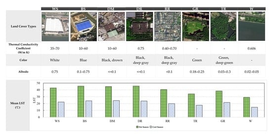
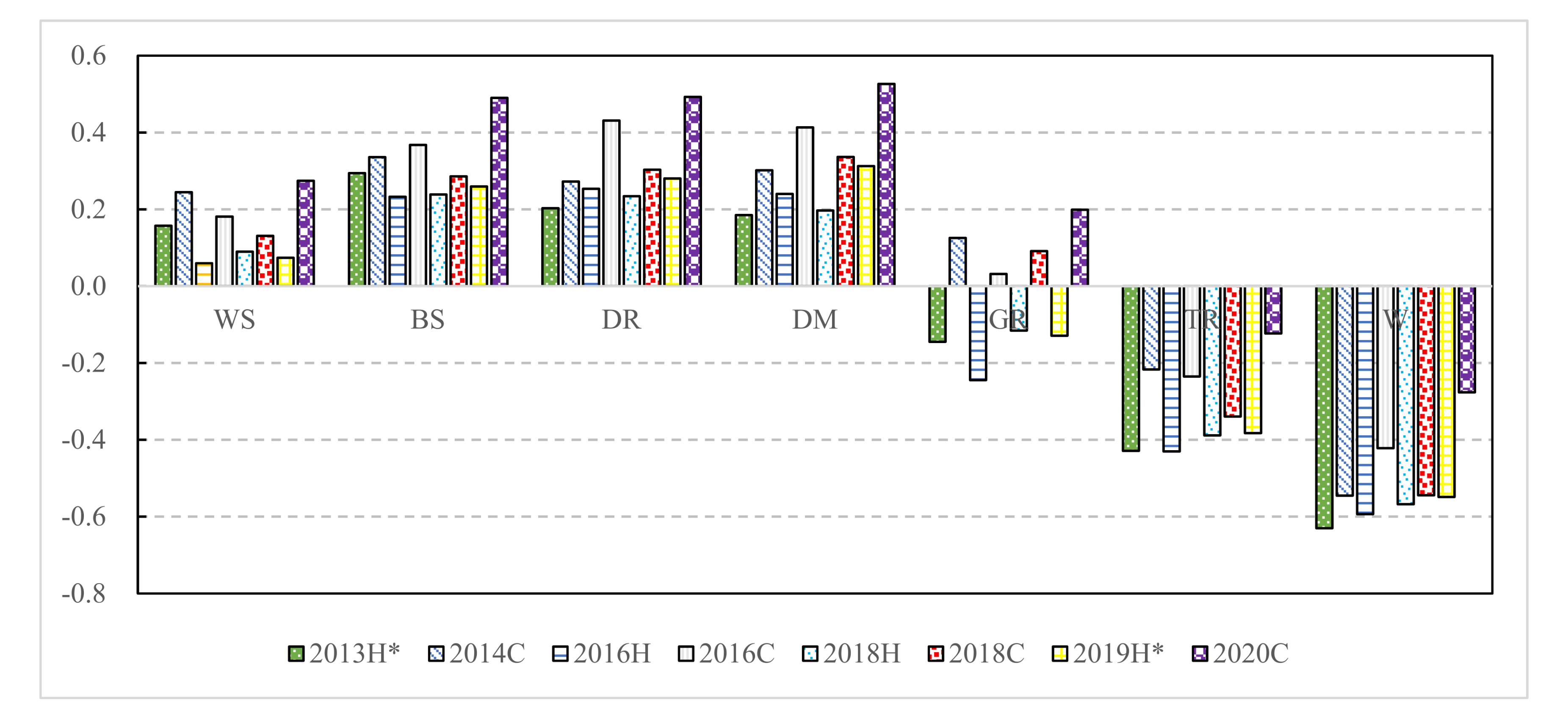
The results of this study demonstrate that various finer ISA classes showed different heat characteristics and thus differed in their contribution to LST. The LSTs of BS and DM were much higher than those of WS, RR, and the pervious surface classes. BS and DM had similar thermal conductivity coefficients around 10–60 (W/m K) at 25 °C (Table 2) [27]. This means they may heat up rapidly when they absorb energy from the sun. The LSTs of DR and DM were much higher than those of WS and RR; DM had the highest impact on high LST values, whereas WS showed the least heating effect as per the corresponding regression coefficients. These results may be due to their low albedo characteristics (close to 0.1); this pattern aligns with the color of absorbing heat, where black > white. Black materials are able to absorb more heat than white materials under the same environmental conditions, as white-colored materials reflect more solar energy than materials with other colors [22,25,39].

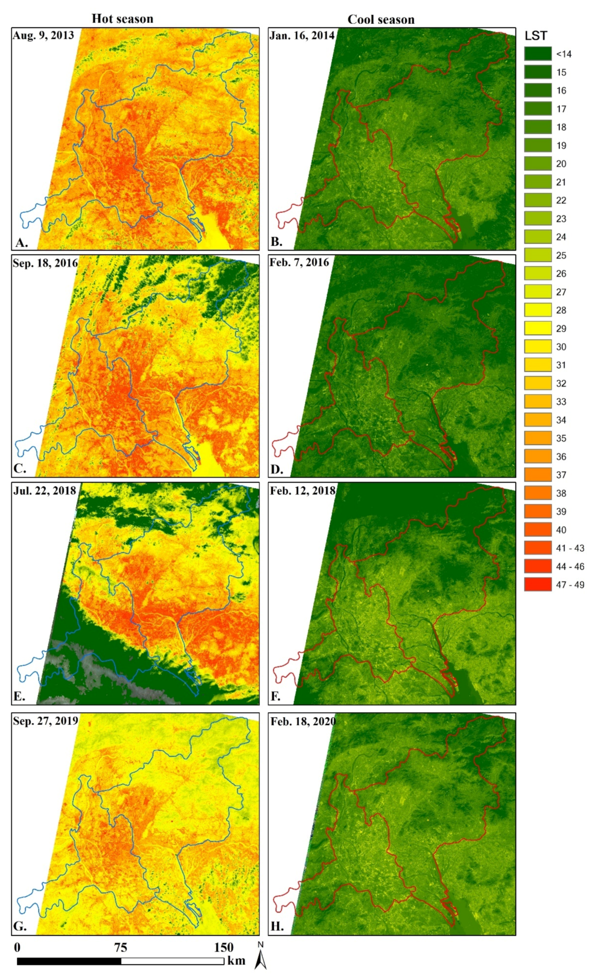
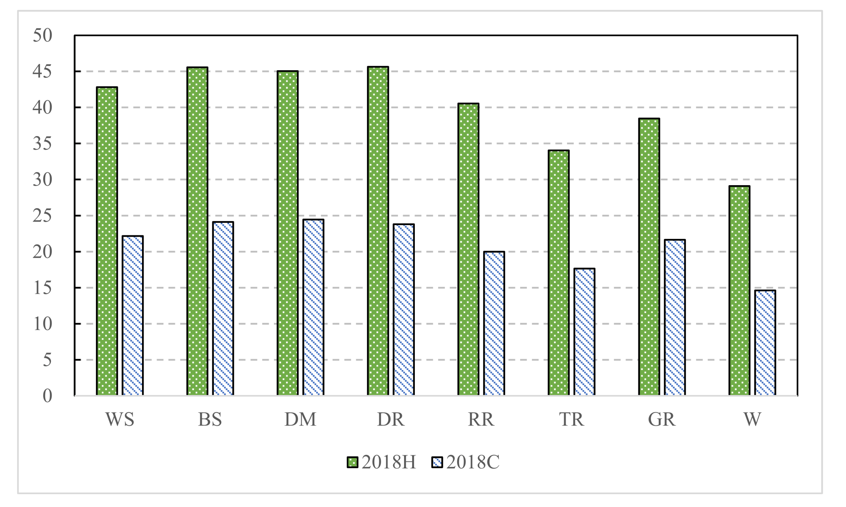
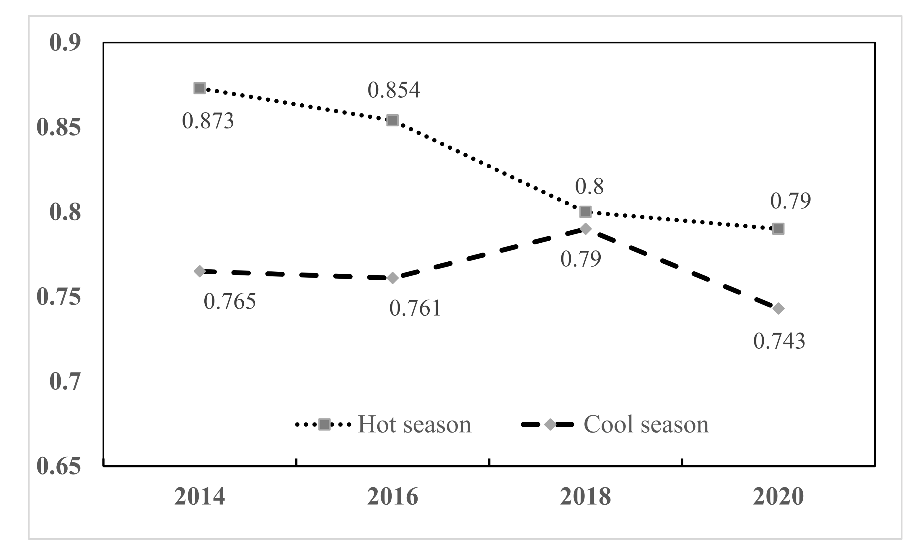
The influence of different surface materials on LST varied during the hot and cool seasons. The impact magnitudes of finer ISA classes were more substantial during the cool season, although they were weaker than those of vegetation and water during the hot season (Figure 10). Some studies have concluded that the radiation intensity of an ISA increases in the summer compared to other seasons, resulting in an increased albedo and a corresponding reduction in LST [39,40,41]. By contrast, rural areas experienced an increase in temperature that was up to 0.27 °C during the summer [42]. An additional factor that affected the LST contribution of finer classes was the moisture content of air between seasons. Air was less humid during the cool season than the hot season, reducing the surface heat capacity and increasing the surface heat radiation during the former [43,44]. Therefore, the contribution of finer ISAs to LST was weaker during the hot season than the cool season.

Parameters such as building density, average building height, and distance to the city center were used in the regression analysis. Most research to date has demonstrated that the horizontal and vertical differences in three-dimensional cities have an impact on LST. Many researchers have often linked building height to the urban shadow; the higher the building, the lower the temperature in this area due to the effect of shadows [45,46]. However, there was also a significant positive correlation between building density and LST during the hot season, and a negative correlation during the cool season. This is related to the monsoon climate, building ventilation, and human activities during different seasons [47,48].

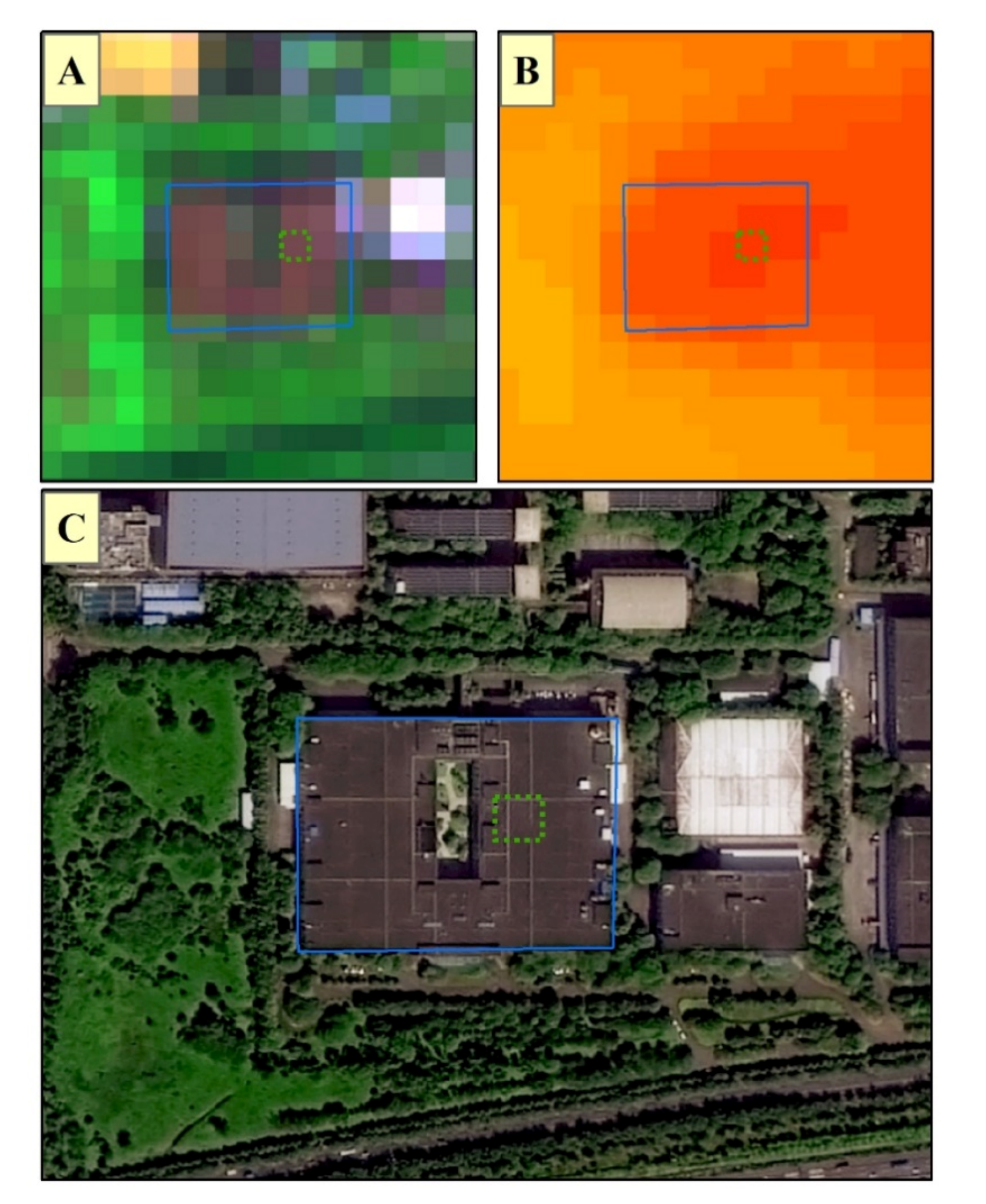
There were four key limitations in this current study. First, only five types of building roofs were discussed because of the limited sample collection within the study area. Finer ISA classes, such as brick, stone, and plastic, should be collected for analysis in future studies. Second, the analysis of the impact of finer ISA classes on LST was limited to daytime imagery, particularly 11:00 a.m. local time. These impacts may vary during the afternoon or nighttime. Moreover, this research focused on the relationship between finer ISA classes and LST; however, the factors that affect urban LST are complex, including urban three-dimensional space, urban functional area distribution, and heat emissions from human activities. At the same time, LST was closely related to surface energy balance (SEB); thus, it is recommended that future research analyze the changes and driving factors of urban LST within a multi-dimensional context. Third, the analysis method used only accommodates multiple regression; as such, a new method of comparative analysis is required in future research to fully reflect the relationship between each finer roof class and the LST. Finally, shadows may have an important effect on the LST. During the sampling process, we selected samples with no or limited shadowed areas. While shadow areas were not removed during the data pre-processing stage of this study, this step should be considered in future studies.

6. Conclusions

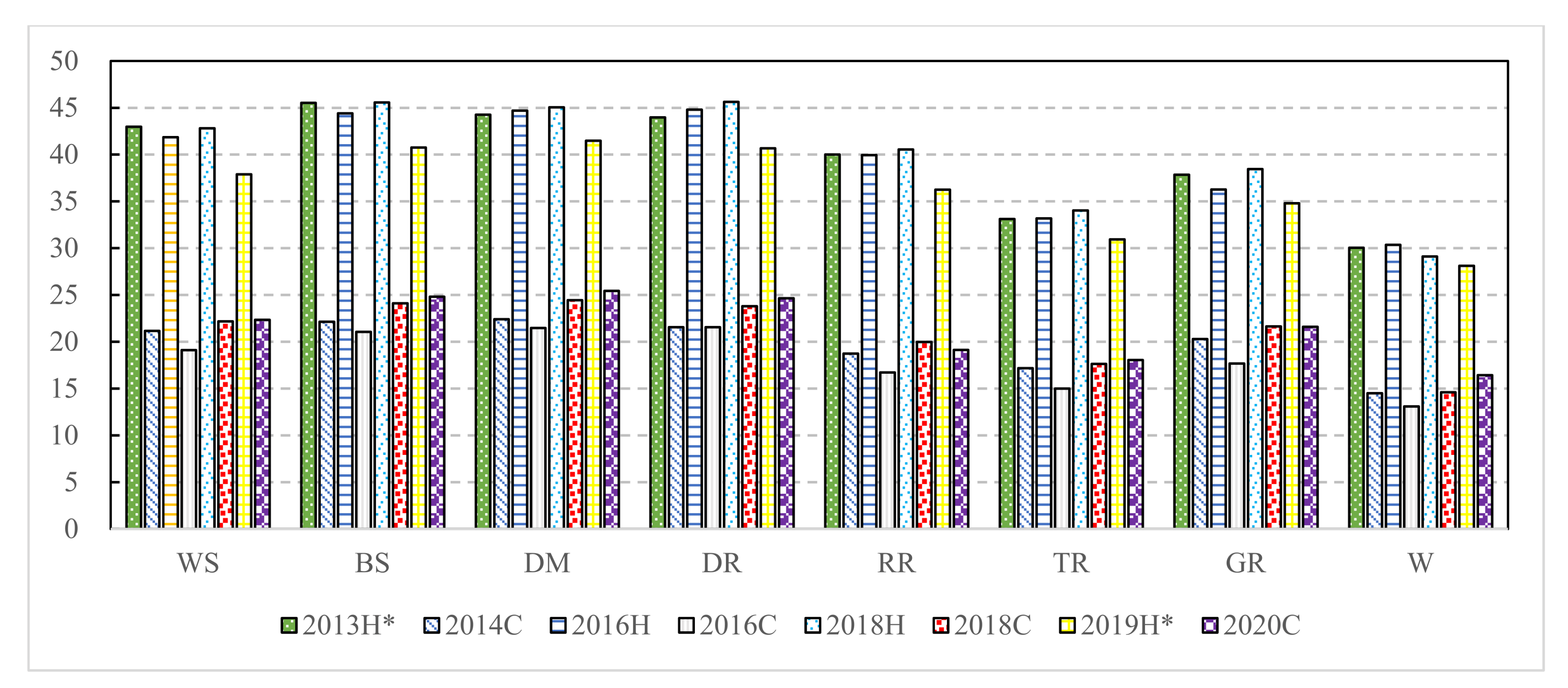
This study discussed the impacts of finer ISA classes on LST and their temporal variations. Bar charts and ANOVA were used to demonstrate the different LST characteristics of each class. Multivariate regression models were applied to selected variables (where RR was set as the reference) during the hot and cool seasons for 2014, 2016, 2018, and 2020. The key findings from the analysis were:

(1)

The mean LST of different types of building roofs were statistically different from each other; these differences were stronger during the hot season than the cool season. The LST of WS was significantly different from that of BS, DM, DR, and RR. The mean LSTs of BS, DM, and DR were significantly higher than those of WS and RR.

(2)

The impacts of building roof types on the LST differed. WS, BS, DR, and DM were positively correlated with LST, while RR was negatively correlated with LST during the cool season. The impact of WS on LST was significantly different from that of BS, DR, DM, and RR. The impacts of the finer ISA classes of BS, DR, and DM on LSTs were similar; however, they demonstrated a consistent descending order pattern (i.e., DM > BS > DR >WS), during the cool season.

(3)

The contributions of finer ISA classes to LST variance were stronger during the cool season than the hot season, as their standardized coefficients were larger in the former than the latter.

This study provides useful information to mitigate the UHI effect by unveiling specific urban heat retention drivers within urban areas. This includes different types of building roofs and pervious surface classes. This information may assist policymakers in developing effective measurements to deal with the UHI phenomenon and related health concerns.

References

1. Peng, J.; Jia, J.; Liu, Y.; Li, H.; Wu, J. Seasonal contrast of the dominant factors for spatial distribution of land surface temperature in urban areas. Remote Sens. Environ. 2018, 215, 255–267. [Google Scholar] [CrossRef]
2. Liu, Y.; Huang, X.; Yang, Q.; Cao, Y. The turning point between urban vegetation and artificial surfaces for their competitive effect on land surface temperature. J. Clean. Prod. 2021, 292, 126034. [Google Scholar] [CrossRef]
3. Waseem, S.; Khayyam, U. Loss of vegetative cover and increased land surface temperature: A case study of Islamabad, Pakistan. J. Clean. Prod. 2019, 234, 972–983. [Google Scholar] [CrossRef]
4. Liu, X.; Zhou, Y.; Yue, W.; Li, X.; Liu, Y.; Lu, D. Spatiotemporal patterns of summer urban heat island in Beijing, China using an improved land surface temperature. J. Clean. Prod. 2020, 257, 120529. [Google Scholar] [CrossRef]
5. Meng, Q.; Zhang, L.; Sun, Z.; Meng, F.; Wang, L.; Sun, Y. Characterizing spatial and temporal trends of surface urban heat island effect in an urban main built-up area: A 12-year case study in Beijing, China. Remote Sens. Environ. 2018, 204, 826–837. [Google Scholar] [CrossRef]
6. Yang, J.; Wang, Y.; Xiu, C.; Xiao, X.; Xia, J.; Jin, C. Optimizing local climate zones to mitigate urban heat island effect in human settlements. J. Clean. Prod. 2020, 275, 123767. [Google Scholar] [CrossRef]
7. He, X.; Wang, J.; Feng, J.; Yan, Z.; Miao, S.; Zhang, Y.; Xia, J. Observational and modeling study of interactions between urban heat island and heatwave in Beijing. J. Clean. Prod. 2020, 247, 119169. [Google Scholar] [CrossRef]
8. Liu, N.; Morawska, L. Modeling the urban heat island mitigation effect of cool coatings in realistic urban morphology. J. Clean.Prod. 2020, 264, 121560. [Google Scholar] [CrossRef]
9. Deng, Y.; Wang, S.; Bai, X.; Tian, Y.; Wu, L.; Xiao, J.; Chen, F.; Qian, Q. Relationship among land surface temperature and LUCC, NDVI in typical karst area. Sci. Rep. 2018, 8, 1–12. [Google Scholar] [CrossRef]
10. Zhaoliang, L.; Sibo, D.; Bohui, T.; Hua, W.; Huazhong, R.; Guangjian, Y.; Ronglin, T.; Pei, L. Review of methods for land surface temperature derived from thermal infrared remotely sensed data. J. Remote Sens. 2016, 20, 899–920. [Google Scholar]
11. Yuan, F.; Bauer, M.E. Comparison of impervious surface area and normalized difference vegetation index as indicators of surface urban heat island effects in Landsat imagery. Remote Sens. Environ. 2007, 106, 375–386. [Google Scholar] [CrossRef]
12. Guo, G.; Wu, Z.; Xiao, R.; Chen, Y.; Liu, X.; Zhang, X. Impacts of urban biophysical composition on land surface temperature in urban heat island clusters. Landsc. Urban Plan. 2015, 135, 1–10. [Google Scholar] [CrossRef]
13. Peng, J.; Xie, P.; Liu, Y.; Ma, J. Urban thermal environment dynamics and associated landscape pattern factors: A case study in the Beijing metropolitan region. Remote Sens. Environ. 2016, 173, 145–155. [Google Scholar] [CrossRef]
14. Sailor, D.J. Simulated Urban Climate Response to Modifications in Surface Albedo and Vegetative Cover. J. Appl. Meteorol. 1995, 34, 1694–1704. [Google Scholar] [CrossRef] [Green Version]
15. Arnfield, A.J. Two decades of urban climate research: A review of turbulence, exchanges of energy and water, and the urban heat island. Int. J. Clim. 2003, 23, 1–26. [Google Scholar] [CrossRef]
16. Lazzarini, M.; Marpu, P.R.; Ghedira, H. Temperature-land cover interactions: The inversion of urban heat island phenomenon in desert city areas. Remote. Sens. Environ. 2013, 130, 136–152. [Google Scholar] [CrossRef]
17. Deilami, K.; Kamruzzaman, M.; Liu, Y. Urban heat island effect: A systematic review of spatio-temporal factors, data, methods, and mitigation measures. Int. J. Appl. Earth Obs. Geoinf. 2018, 67, 30–42. [Google Scholar] [CrossRef]
18. Oke, T.R.; Mills, G.; Christen, A.; Voogt, J.A. Urban Climates; Cambridge University Press: Cambridge, UK, 2017. [Google Scholar]
19. Myint, S.W.; Wentz, E.A.; Brazel, A.J. The impact of distinct anthropogenic and vegetation features on urban warming. Landsc. Ecol. 2013, 28, 959–978. [Google Scholar] [CrossRef] [Green Version]
20. Administration, C.M. Historical Temperature in Guangzhou. Available online: http://lishi.tianqi.com/guangzhou/201401.html (accessed on 1 January 2021).
21. Susca, T.; Gaffin, S.R.; Dell’Osso, G.R. Positive effects of vegetation: Urban heat island and green roofs. Environ. Pollut. 2011, 159, 2119–2126. [Google Scholar] [CrossRef]
22. Synnefa, A.; Santamouris, M.; Livada, I. A study of the thermal performance of reflective coatings for the urban environment. Solar Energy 2006, 80, 968–981. [Google Scholar] [CrossRef]
23. Mitchell, T.P.; Wallace, J.M. The Annual Cycle in Equatorial Convection and Sea Surface Temperature. J. Clim. 1992, 5, 1140–1156. [Google Scholar] [CrossRef] [Green Version]
24. Vallero, D.A. 5—The Physics of the Atmosphere. In Fundamentals of Air Pollution, 4th ed.; Vallero, D.A., Ed.; Academic Press: Cambridge, MA, USA, 2008; pp. 123–153. [Google Scholar] [CrossRef]
25. Simpson, J.R.; McPherson, E.G. The effects of roof albedo modification on cooling loads of scale model residences in Tucson, Arizona. Energy Build. 1997, 25, 127–137. [Google Scholar] [CrossRef]
26. Siegert, M.J. Evidence of the Growth and Decay of Ice Sheets on Glaciated Landscapes. In Reference Module in Earth Systems and Environmental Sciences; Elsevier: Amsterdam, The Netherlands, 2014. [Google Scholar] [CrossRef]
27. ToolBox, E. Thermal Conductivity of Selected Materials and Gases. Available online: https://www.engineeringtoolbox.com/thermal-conductivity-d_429.html (accessed on 29 July 2020).
28. Jiménez-Muñoz, J.C.; Sobrino, J.A. A generalized single-channel method for retrieving land surface temperature from remote sensing data. Journal of Geophysical Research: Atmospheres 2003, 108, 108. [Google Scholar] [CrossRef] [Green Version]
29. Jiménez-Muñoz, J.; Sobrino, J. Error sources on the land surface temperature retrieved from thermal infrared single channel remote sensing data. Int. J. Remote. Sens. 2006, 27, 999–1014. [Google Scholar] [CrossRef]
30. Jiménez-Muñoz, J.C.; Cristóbal, J.; Sobrino, J.A.; Sòria, G.; Ninyerola, M.; Pons, X. Revision of the single-channel algorithm for land surface temperature retrieval from Landsat thermal-infrared data. IEEE Trans. Geosci. Remote. Sens. 2008, 47, 339–349. [Google Scholar] [CrossRef]
31. Oluwapelumi, A. Incorporating dummy variables in regression model to determine the average internally generated revenue and wage bills of the six geopolitical zones in Nigeria. Eur. J. Stat. Probab. 2014, 2, 23–27. [Google Scholar]
32. Wu, X.; Cao, J.; Huting, J. Using three-factor theory to identify improvement priorities for express and local bus services: An application of regression with dummy variables in the Twin Cities. Transp. Res. Part A Policy Pract. 2018, 113, 184–196. [Google Scholar] [CrossRef]
33. Mackiewicz, M.C. A new approach to quantifying soil temperature responses to changing air temperature and snow cover. Polar Sci. 2012, 6, 226–236. [Google Scholar] [CrossRef] [Green Version]
34. Miller, J.L.L.; Erickson, M.L. On dummy variable regression analysis: A description and illustration of the method. Sociol. Methods Res. 1974, 2, 409–430. [Google Scholar] [CrossRef]
35. Hardy, M.A. Regression with Dummy Variables; Sage, Inc.: Newbury Park, CA, USA, 1993; Volume 93. [Google Scholar]
36. Fumo, N.; Biswas, M.A.R. Regression analysis for prediction of residential energy consumption. Renew. Sustain. Energy Rev. 2015, 47, 332–343. [Google Scholar] [CrossRef]
37. Shams, S.R.; Jahani, A.; Kalantary, S.; Moeinaddini, M.; Khorasani, N. Artificial intelligence accuracy assessment in NO2 concentration forecasting of metropolises air. Sci. Rep. 2021, 11, 1–9. [Google Scholar] [CrossRef]
38. Yan, L.; Zhengquan, C.; Meng, Y. Climatic Characteristics of Guangzhou Temperature and Its Cause Analysis. Meteorol. Mon. 2008, 2, 52–60. [Google Scholar]
39. Menon, S.; Akbari, H.; Mahanama, S.; Sednev, I.; Levinson, R. Radiative forcing and temperature response to changes in urban albedos and associated CO2 offsets. Environ. Res. Lett. 2010, 5, 014005. [Google Scholar] [CrossRef]
40. Taha, H. Meso-urban meteorological and photochemical modeling of heat island mitigation. Atmos. Environ. 2008, 42, 8795–8809. [Google Scholar] [CrossRef]
41. Synnefa, A.; Saliari, M.; Santamouris, M. Experimental and numerical assessment of the impact of increased roof reflectance on a school building in Athens. Energy Build. 2012, 55, 7–15. [Google Scholar] [CrossRef]
42. Millstein, D.; Menon, S. Regional climate consequences of large-scale cool roof and photovoltaic array deployment. Environ. Res. Lett. 2011, 49123, 98–204. [Google Scholar] [CrossRef]
43. Taha, H.; Sailor, D.; Akbari, H. High-Albedo Materials for Reducing Building Cooling Energy Use; U.S. Department of Energy Office of Scientific and Technical Information: Oak Ridge, TN, USA, 1992.
44. Oke, T.R. Boundary Layer Climates. Earth Sci. Rev. 1987, 27, 265. [Google Scholar]
45. Li, T.; Cao, J.; Xu, M.; Wu, Q.; Yao, L. The influence of urban spatial pattern on land surface temperature for different functional zones. Landsc. Ecol. Eng. 2020, 16, 249–262. [Google Scholar] [CrossRef]
46. Zheng, Z.; Zhou, W.; Yan, J.; Qian, Y.; Wang, J.; Li, W. The higher, the cooler? Effects of building height on land surface temperatures in residential areas of Beijing. Phys. Chem. Earth Parts A/B/C 2019, 110, 149–156. [Google Scholar] [CrossRef]
47. Yang, J.; Jin, S.; Xiao, X.; Jin, C.; Xia, J.C.; Li, X.; Wang, S. Local climate zone ventilation and urban land surface temperatures: Towards a performance-based and wind-sensitive planning proposal in megacities. Sustain. Cities Soc. 2019, 47, 101487. [Google Scholar] [CrossRef]
48. Guo, G.; Zhou, X.; Wu, Z.; Xiao, R.; Chen, Y. Characterizing the impact of urban morphology heterogeneity on land surface temperature in Guangzhou, China. Environ. Model. Softw. 2016, 84, 427–439. [Google Scholar] [CrossRef]
Figure 1. Study areas: cities of Guangzhou and Foshan. False color image (red: near infrared band; green: red band; blue: green band).
Remotesensing 13 02840 g001
Figure 2. Selected Landsat 8 OLI and the related cloud cover areas. Years of 2013 and 2019 are the substitutes of the hot season in 2014 and 2020, respectively.
Remotesensing 13 02840 g002
Figure 3. Flowchart of research design. TIRS: Thermal Infrared Sensor; OLI: Operational Land Imager; LST: land surface temperature; ISA: impervious surface area; WS: white surface roof; BS: blue steel roof; DM: dark metal roof; DR: dark material roof; RR: residential roof. DIS: distance to city center; B_D: building density; B_H: average building height; _Z: standardized variables; for example, LST_Z means standardized land surface temperature samples; _D: dummy variables, for example, WS_D means white surface class’s dummy variable.
Remotesensing 13 02840 g003
Figure 4. Different building roofs and natural land cover types. WS: white surface roof; BS: blue steel roof; DM: dark metal roof; DR: other dark material roof; RR: residential roof; TR: tree; GR: grass; W: water.
Remotesensing 13 02840 g004
Figure 5. Example of building roof sample selection and according LST extraction. (A) Landsat image, (B) LST image, (C) high spatial resolution image. Blue solid line rectangle: building roof; green dash line rectangle: selected sample (pixel) in LST image.
Remotesensing 13 02840 g005
Figure 6. LST of selected dates (°C). left column: hot seasons; right column: cool seasons. Row 1: 2014 (hot season: 2013); Row 2: 2016; Row 3: 2018; Row 4: 2020 (hot season: 2019).
Remotesensing 13 02840 g006
Figure 7. Mean LST of each class in 2018.
Remotesensing 13 02840 g007
Figure 8. Mean LST of each class. 2013H* and 2019H* were the substitutes of the hot seasons of 2014 and 2020, respectively.
Remotesensing 13 02840 g008
Figure 9. R2 of multivariate regressions.
Remotesensing 13 02840 g009
Figure 10. Standardized coefficients of land cover classes. 2013H* and 2019H* were the substitutes of the hot seasons of 2014 and 2020, respectively.
Remotesensing 13 02840 g010