
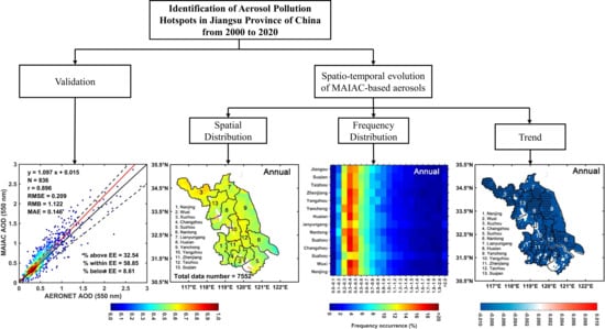
Identification of Aerosol Pollution Hotspots in Jiangsu Province of China

 ,
,  ,
,  , , ,
, , , 
Abstract
:
1. Introduction
2. Materials and Methods
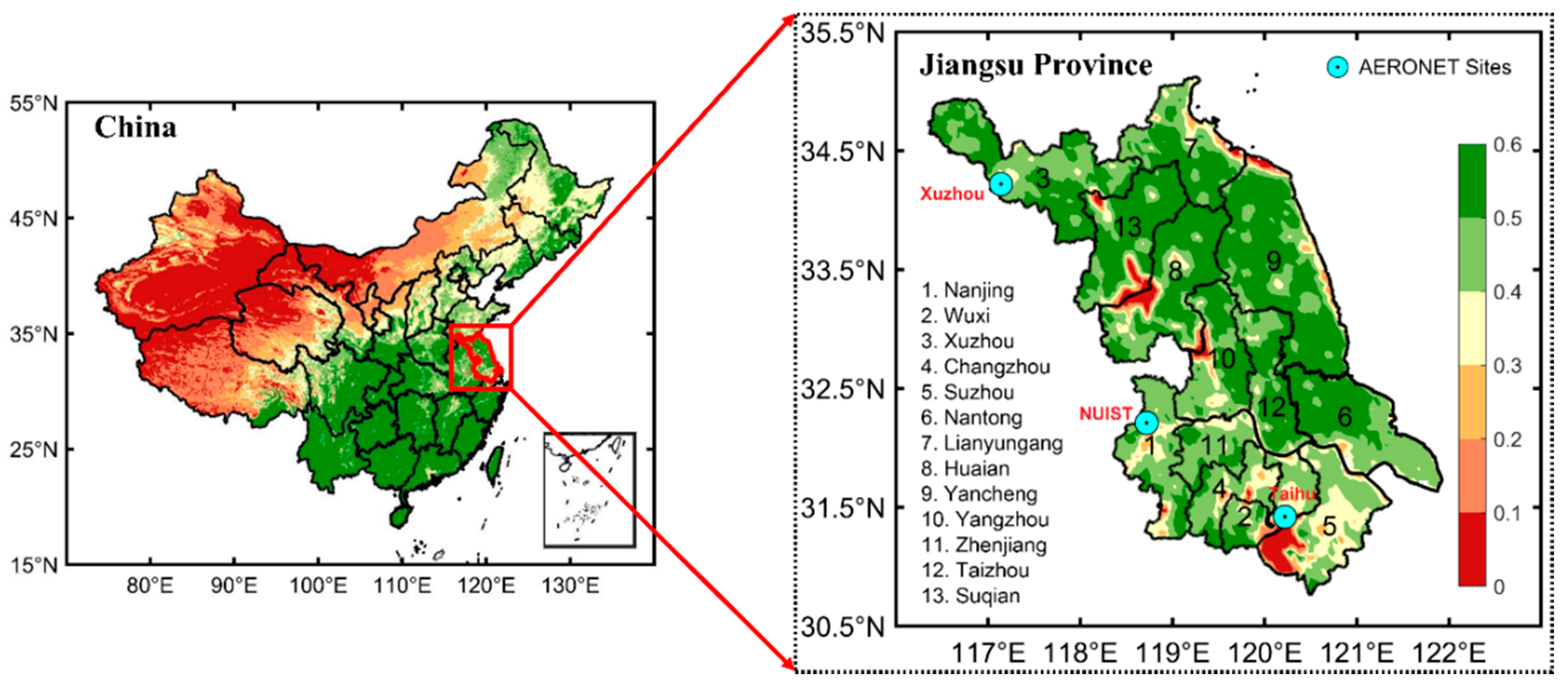
2.1. Study Area
2.2. MAIAC AOD
2.3. AERONET AOD
2.4. Meteorological Data
2.5. Research Methodology
- The study extracted point data from MAIAC AOD using the spatial widow of 3 × 3 pixels surrounding the AERONET sites, which were averaged if at least 2 pixels out of the 9 pixels were available. The AERONET AOD was averaged within a ±60 minute time window from the satellite local time (Terra: 10:30 am, Aqua: 01:30 pm).
- A reduced major axis (RMA) method was used to calculate slope and intercept between the satellite-based MAIAC and AERONET AODs [65]. The slope defines the inaccuracy related to using an imperfect aerosol model, while the intercept implies the inaccuracy related to incorrect surface reflectance calculation [3,66]. In RMA, the following Equations (2) and (3) are used to calculate the slope (β) and intercept (α):where are defined as the means of X and Y, and indicate the standard deviation of X and Y, respectively. A perfect estimation of satellite-based MAIAC AOD is indicated by values of β (=1) and α (=0).
- To determine the uncertainty and accuracy of the satellite-based MAIAC AOD products, this study used the following Equations (4)−(8) for Pearson’s correlation (r), root mean squared error (RMSE), mean absolute error (MAE), relative mean bias (RMB), and expected error envelope (EE) [5,27,67].Here, RMB = 1 defines the normal estimation of MAIAC AOD, while RMB < 1 and > 1 indicates underestimation and overestimation, respectively.
- The Mann–Kendal test was used to calculate the significance of any AOD trends (increasing or decreasing), while Sen’s slope method was used to calculate the magnitude of AOD trends. The methods used in this study are discussed below.
3. Results and Discussion
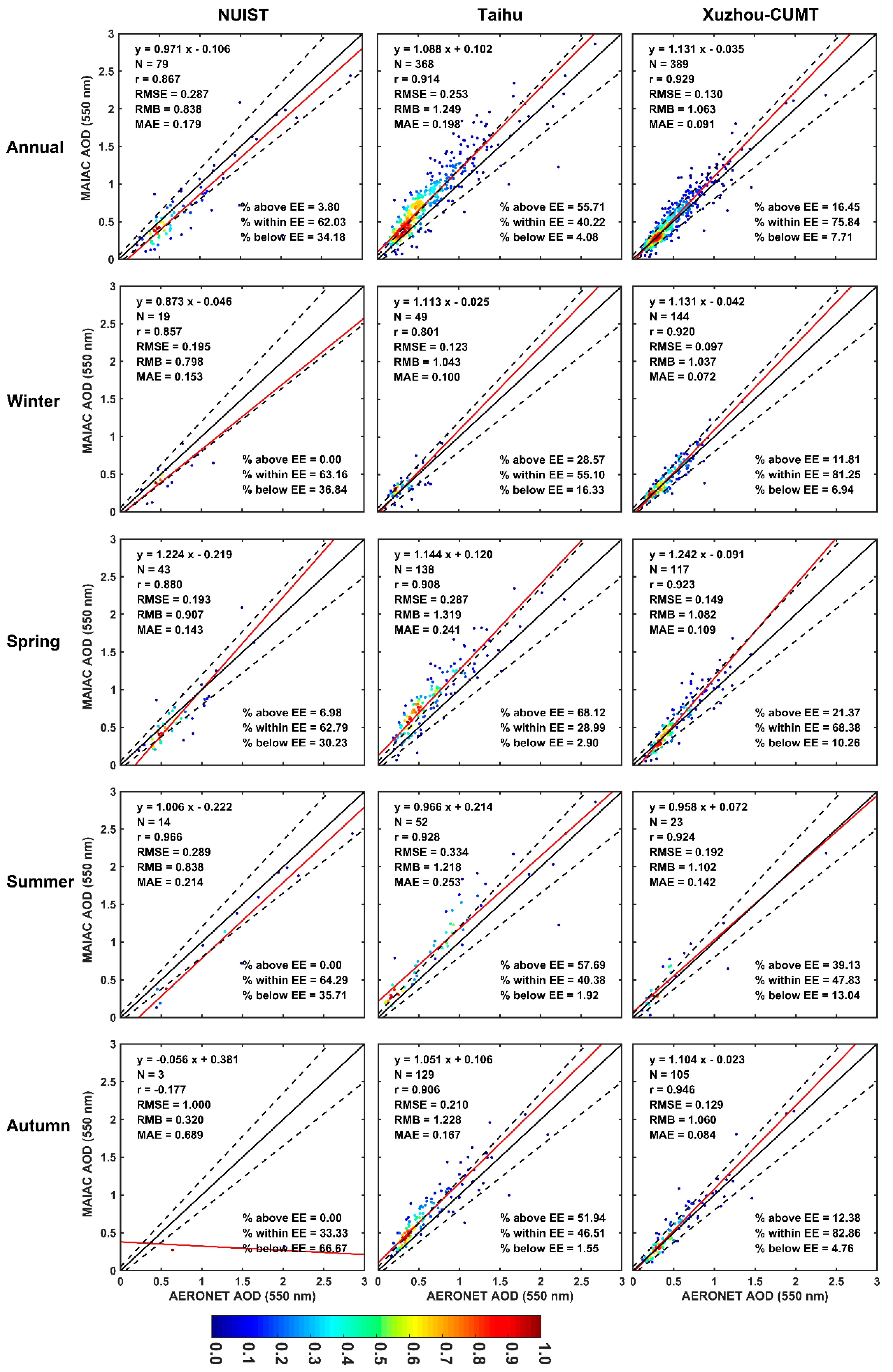
3.1. Evaluations of MAIAC AOD against AERONET AOD
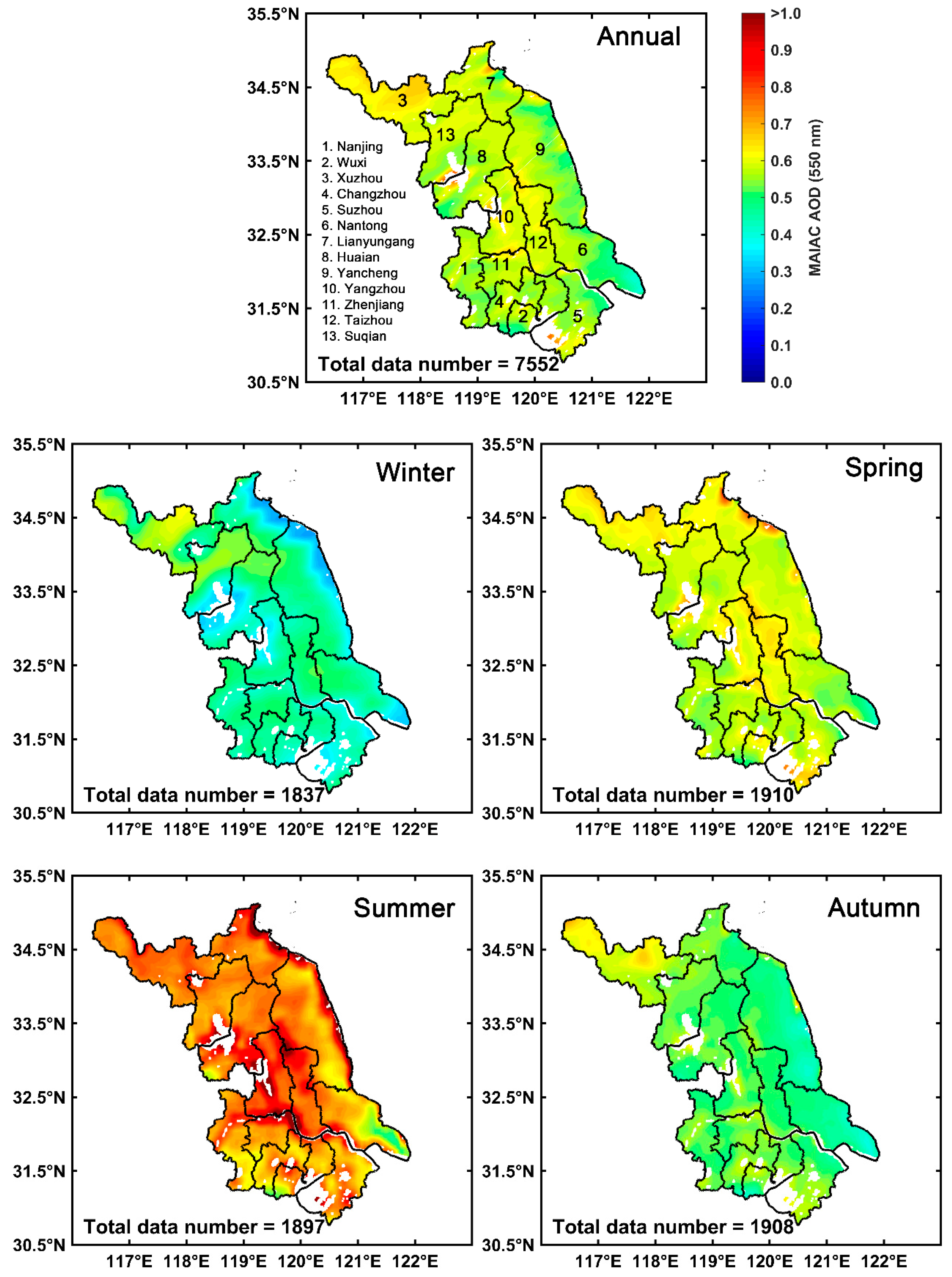
3.2. Spatial Distributions of MAIAC AOD
3.3. Frequency Distribution of AOD
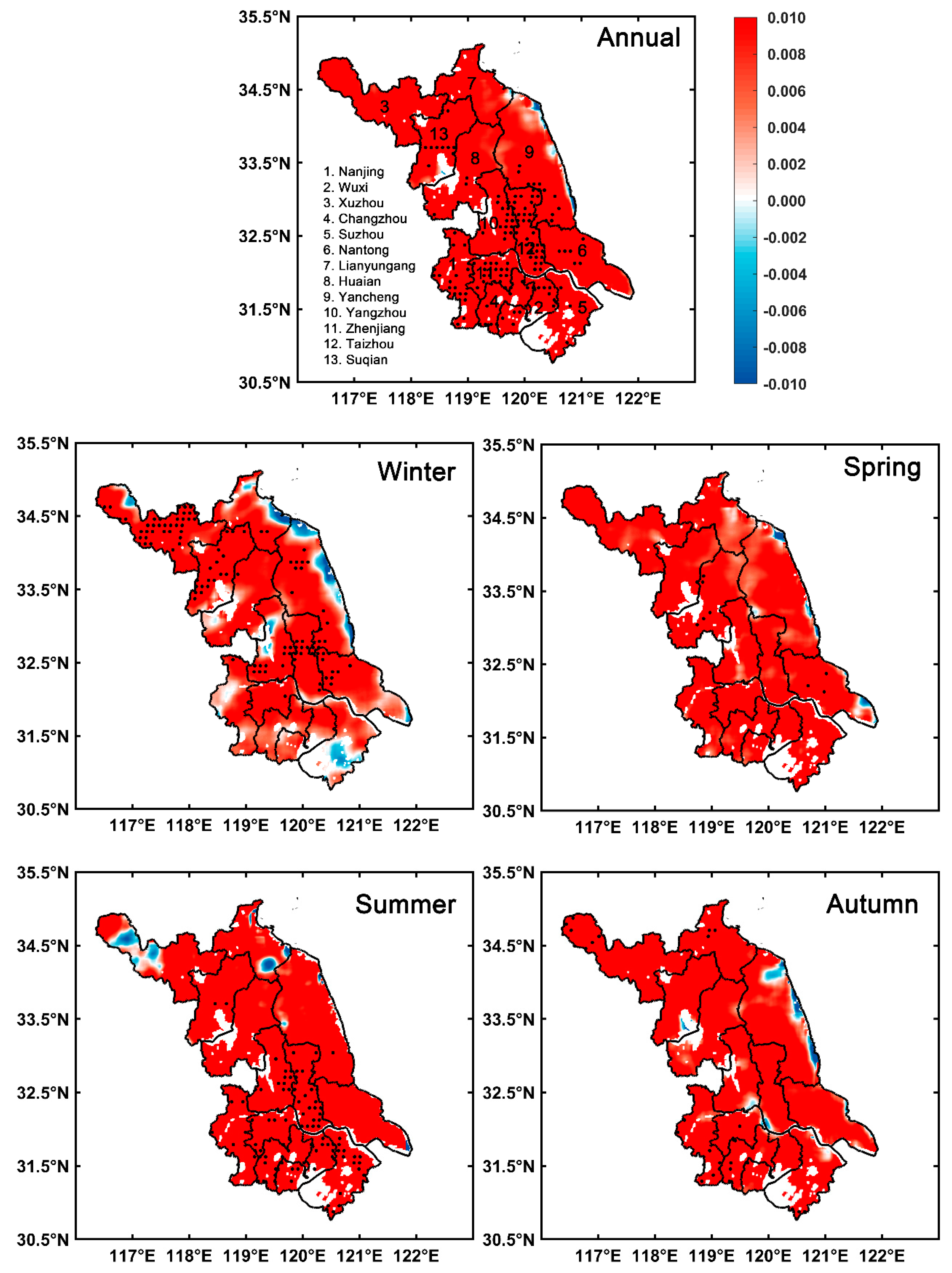
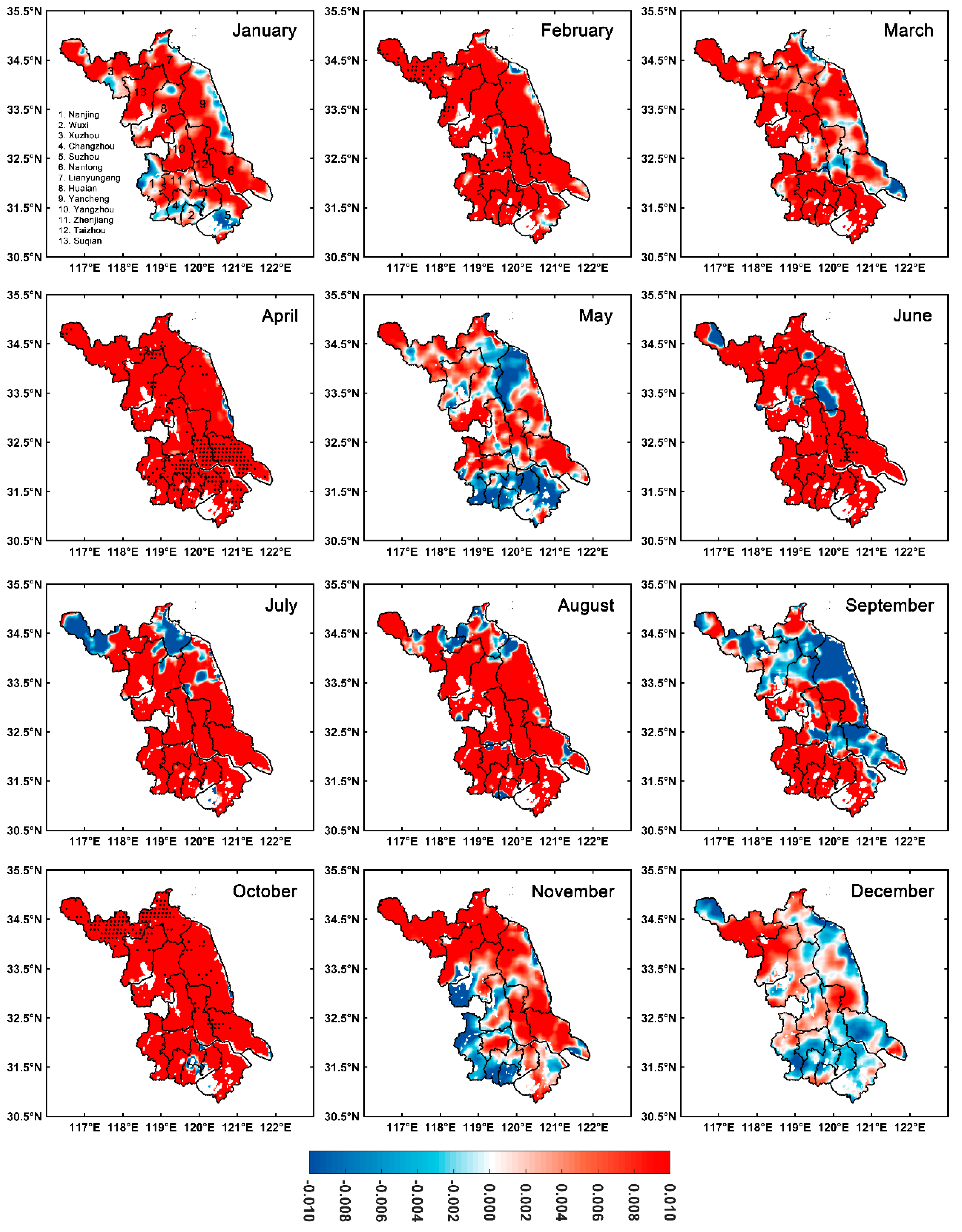
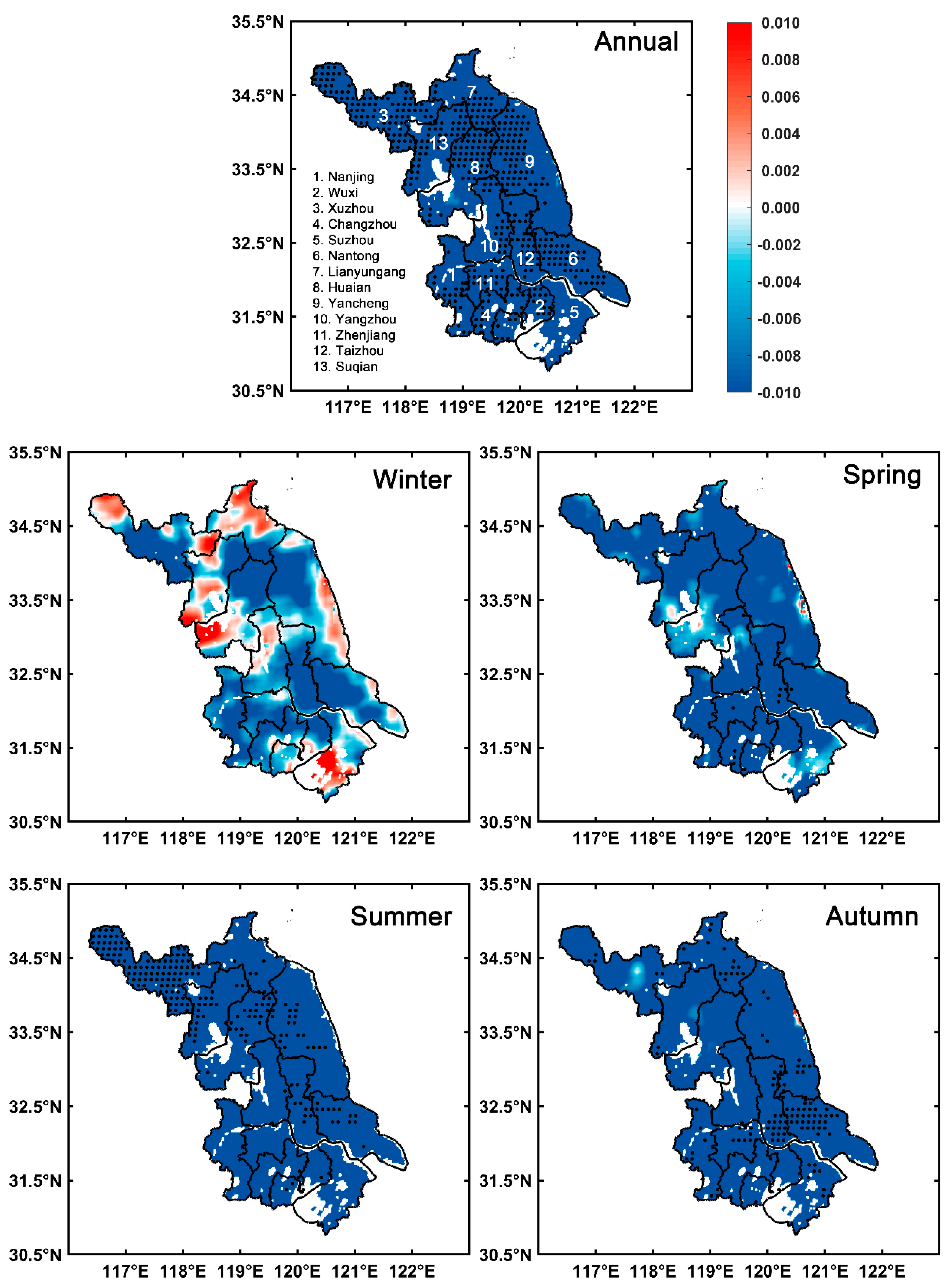
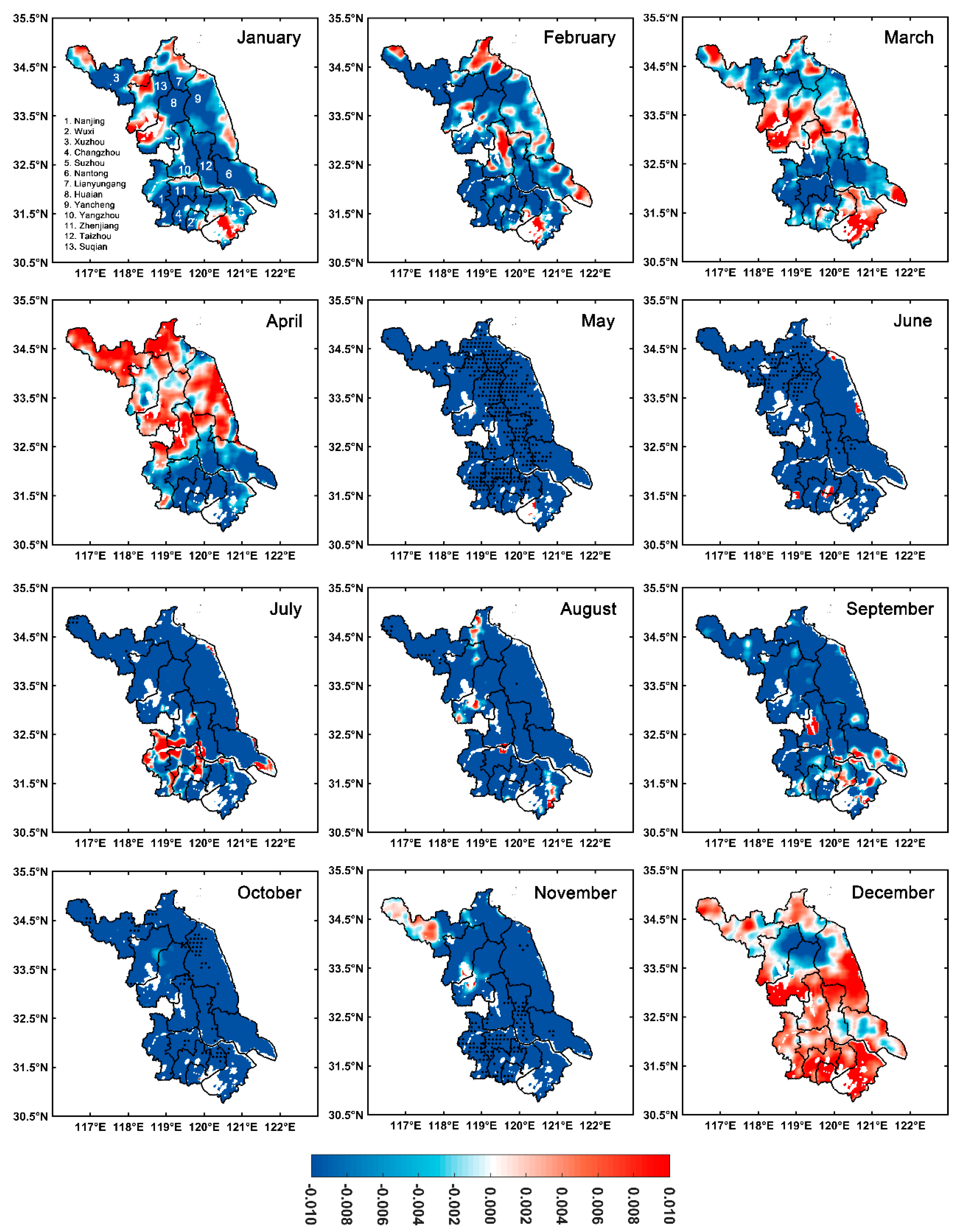
3.4. AOD Trends
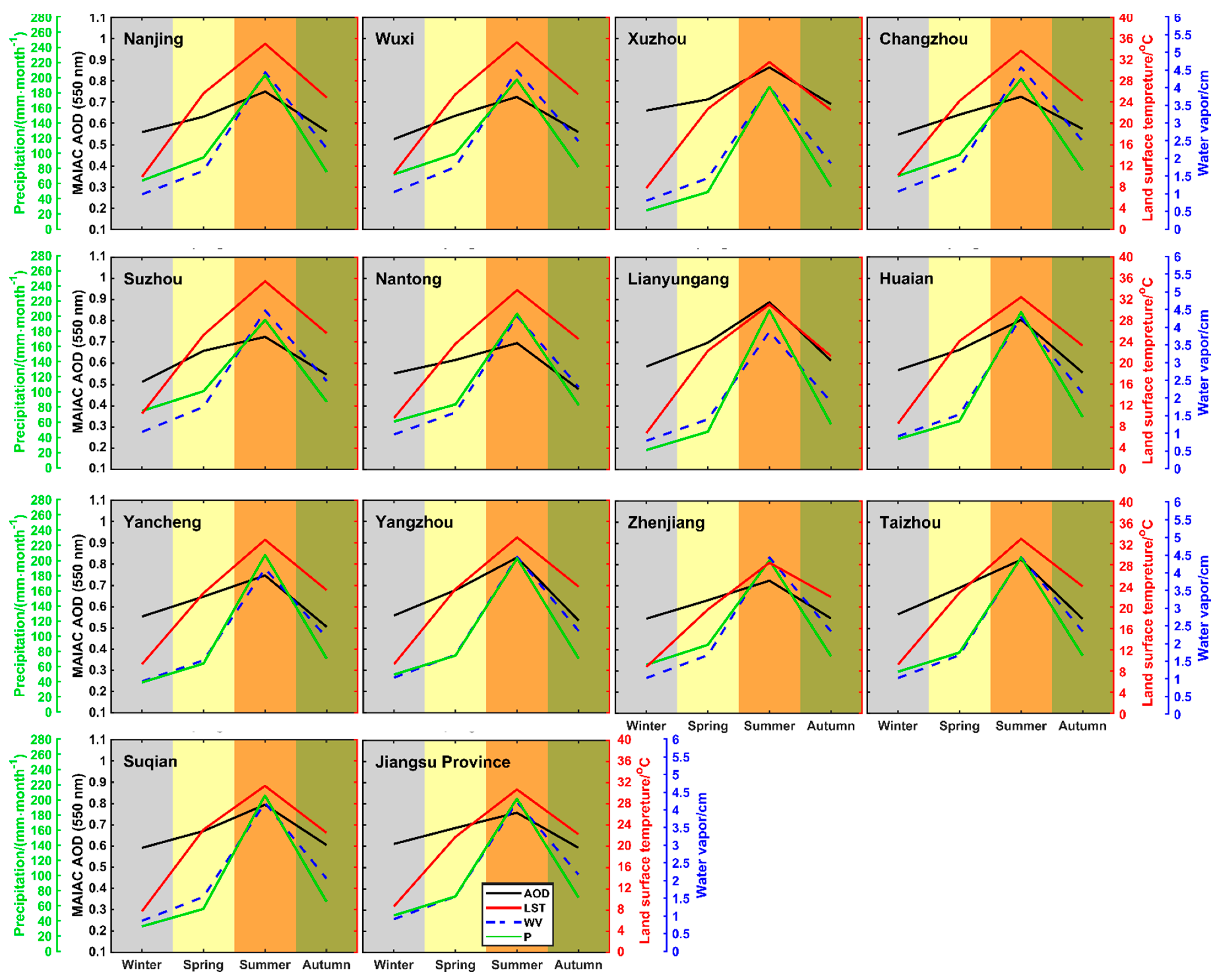
3.5. Relationship between AOD and Meteorological Parameters
4. Conclusions
- The evaluation study showed a consistent result between the MAIAC AOD and AERONET AOD with a high Pearson’s correlation coefficient (r: 0.867~0.929), and lower RMSE (0.130~0.287) and MAE (0.091~0.198). These findings indicate that MODIS high-resolution MAIAC aerosol products can effectively reveal city-level aerosol pollution scenarios.
- The spatial distribution of annual mean AOD showed high values (over 0.60) in most cities, excluding the southeast of Nantong City, which was characterized by a low AOD value (<0.40). Moreover, the 21-year city-level annual mean AOD was highest in Xuzhou (0.73 ± 0.10) and lowest in Nantong (0.59 ± 0.08).
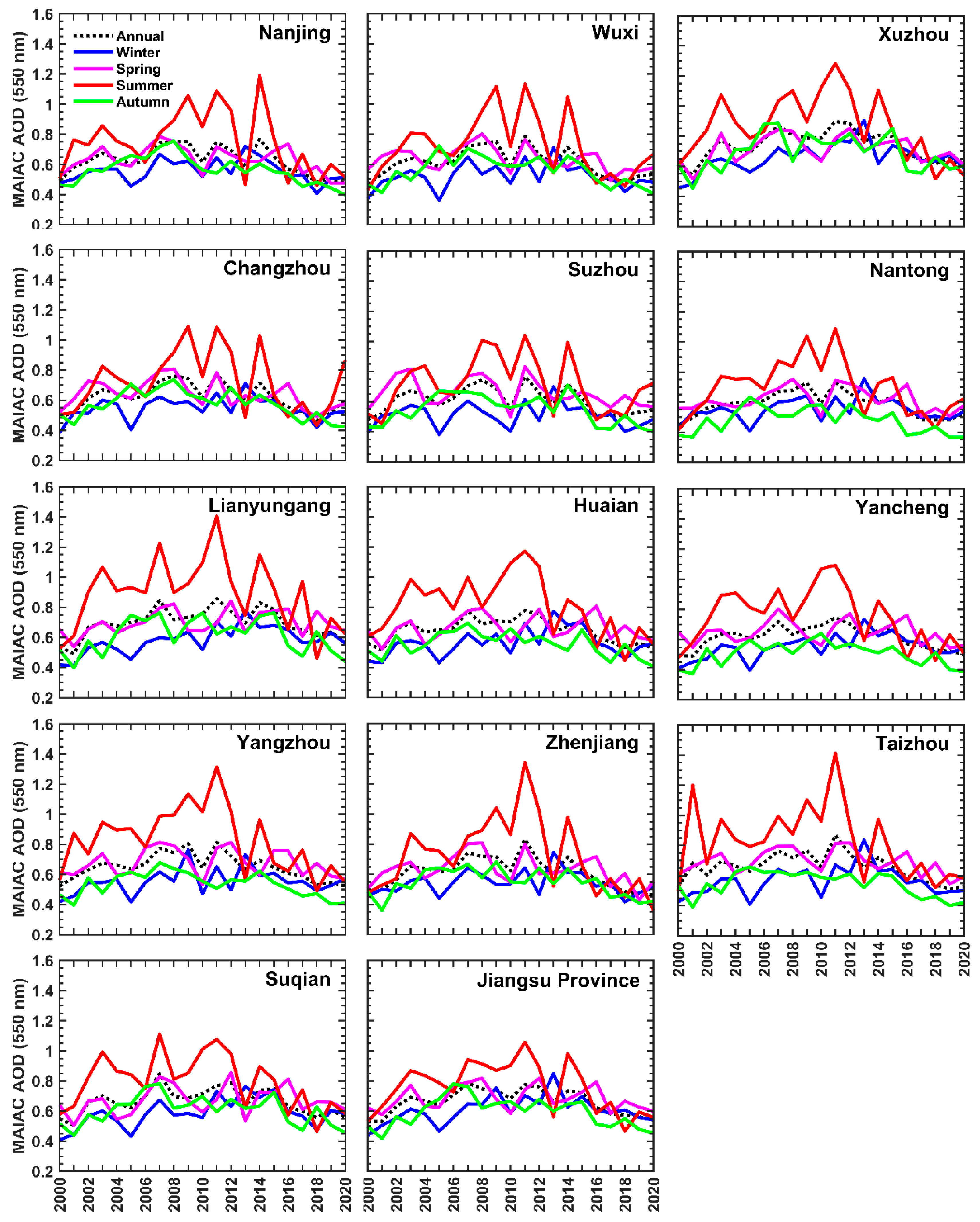
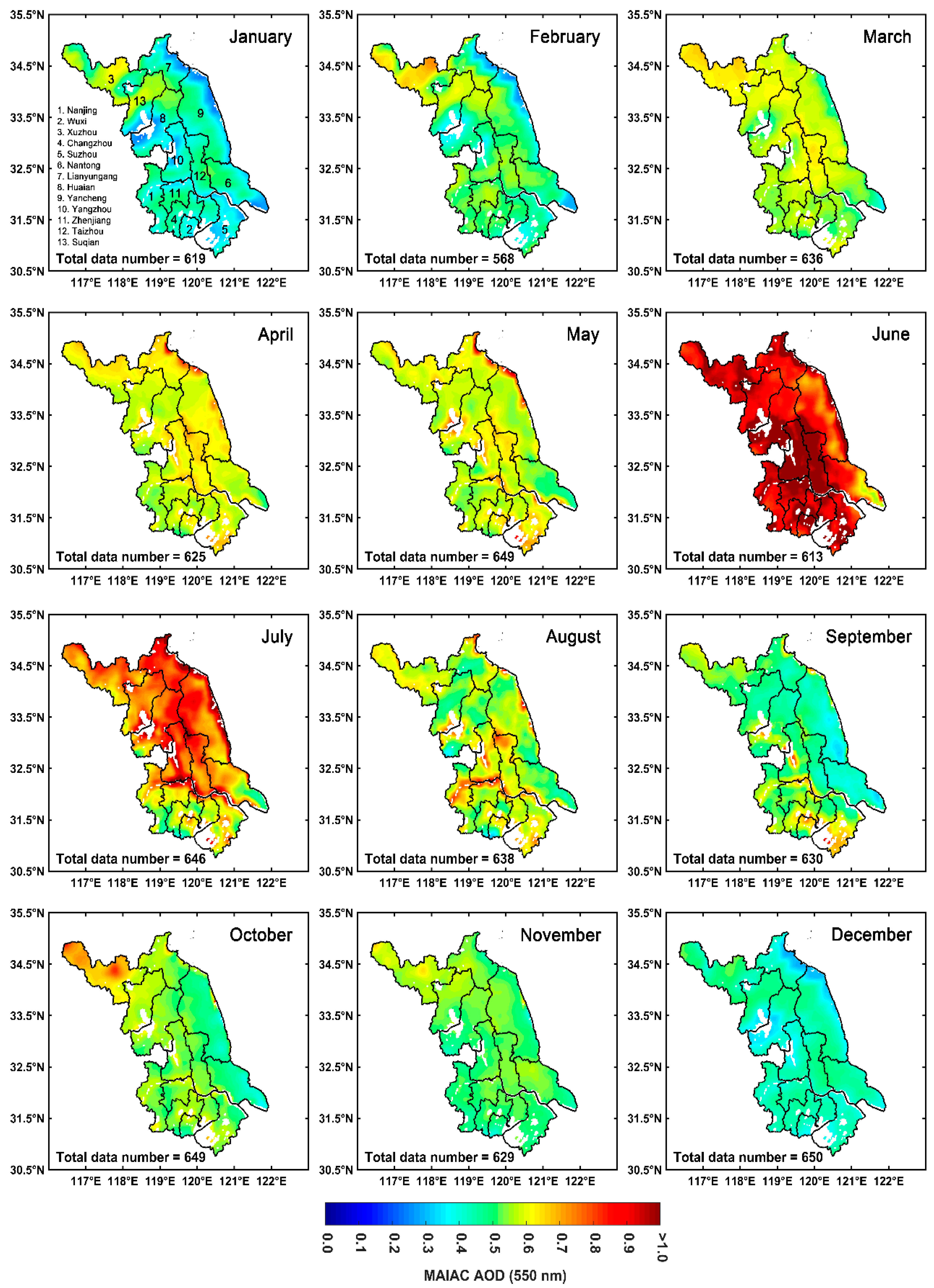
- The spatial distribution of seasonal mean AOD showed higher values in summer (>0.70) than in spring, autumn, and winter for most cities. In particular, the 21-year city-level summer mean AOD was highest in Lianyungang (0.89 ± 0.24) and lowest in Nantong (0.70 ± 0.18), whereas the spring mean AOD was highest in Xuzhou (0.71 ± 0.09) and lowest in Nantong (0.62 ± 0.08). The autumn mean AOD was also highest in Xuzhou (0.69 ± 0.12) and lowest in Nantong (0.48 ± 0.08), whereas winter AOD was highest in Xuzhou (0.66 ± 0.10) and lowest in Suzhou (0.51 ± 0.08). Furthermore, the spatial mean AOD peaked in June (>0.9) and was lowest in December (<0.4) throughout Jiangsu Province.
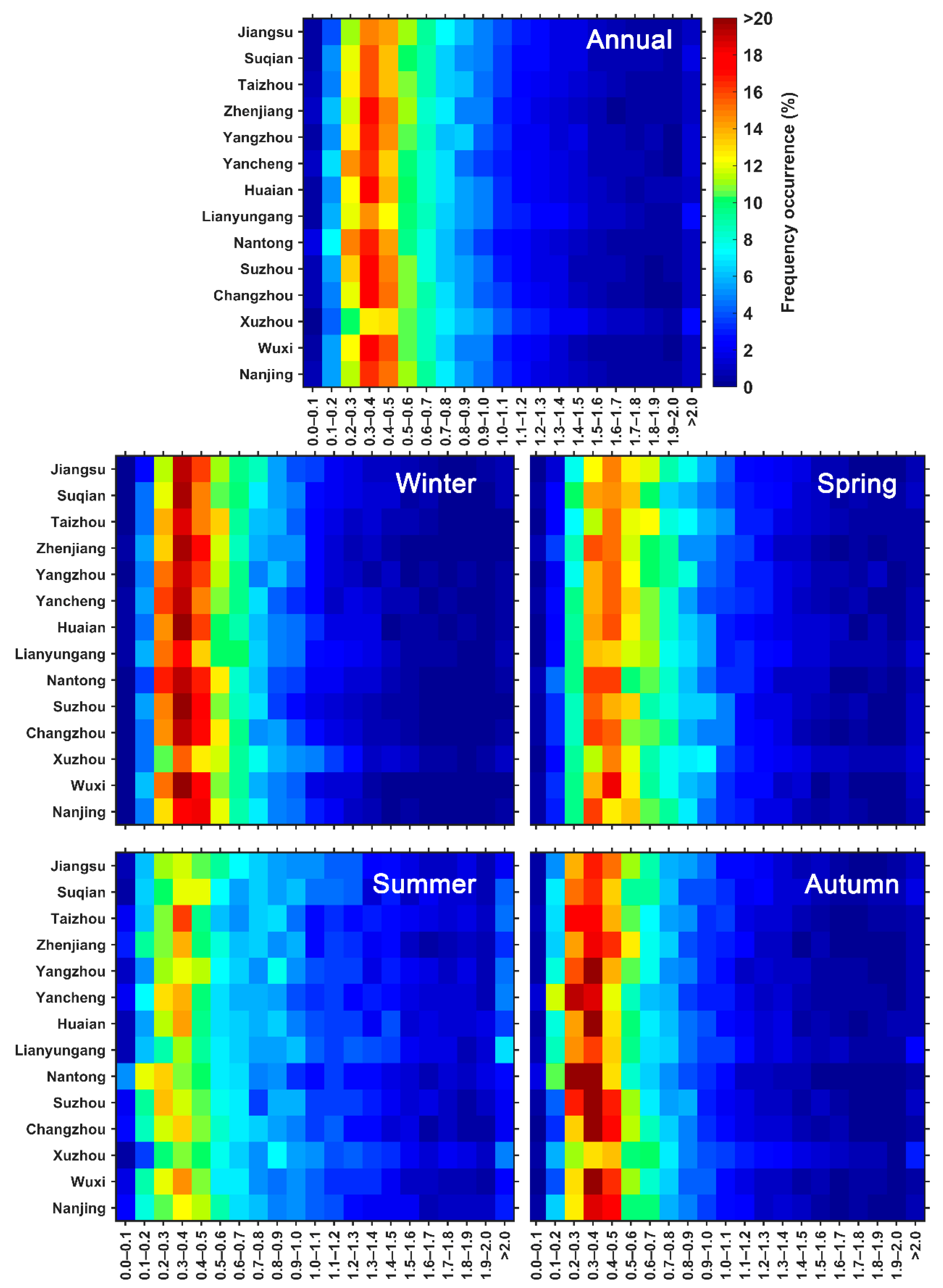
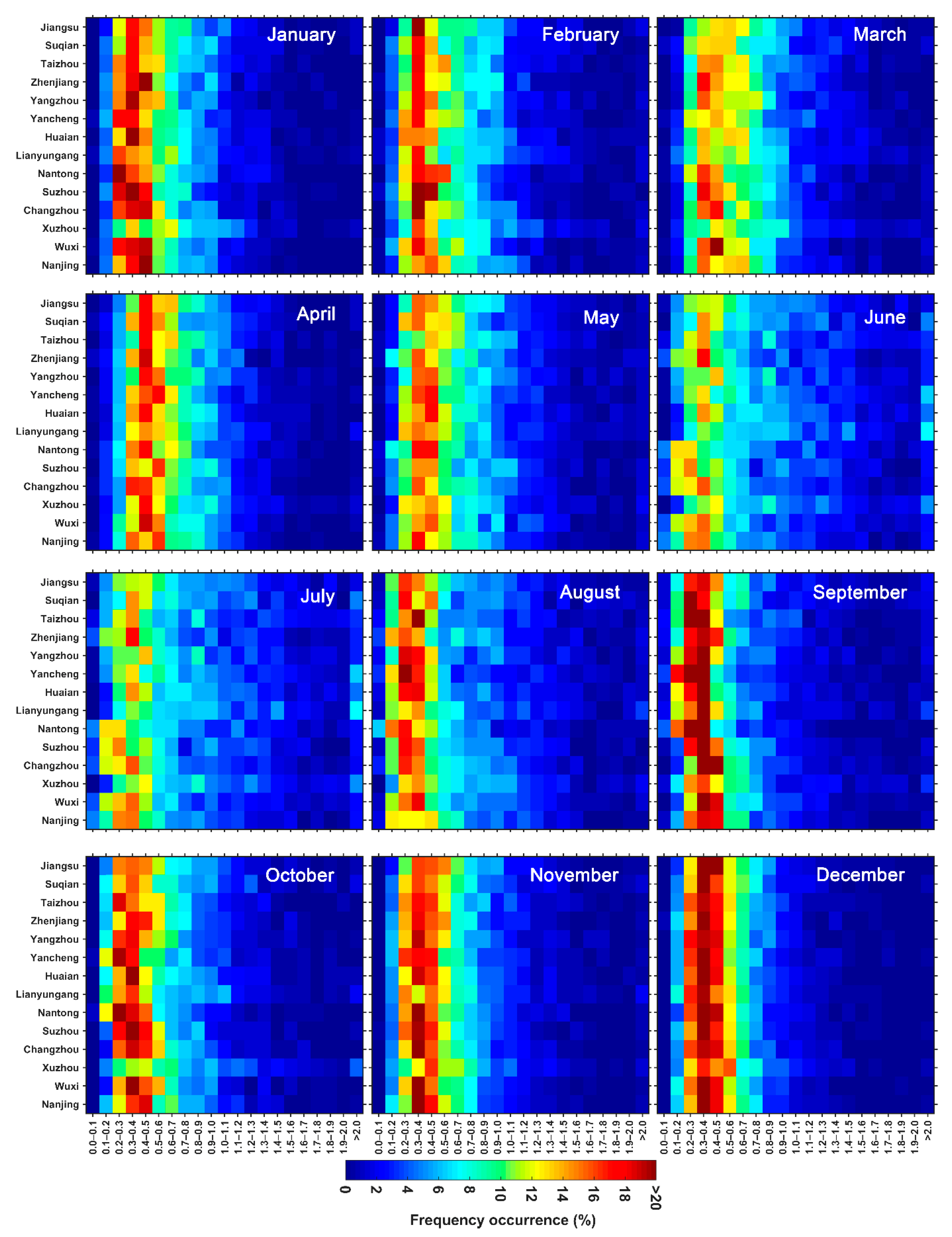
- The occurrence frequencies of 0.3 ≤ AOD < 0.4 and 0.4 ≤ AOD < 0.5 were commonly observed, indicating a turbid atmosphere, perhaps associated with anthropogenic activities, increased emissions, and changes in meteorological circumstances.
- Annually, significant upward AOD trends ranged from 0.016 to 0.028 (per year) in all the 13 cities during 2000–2009, being highest in Changzhou and Yangzhou and lowest in Huaian. Moreover, for 2010–2019, annually, significant downward AOD trends (per year) varied between 0.020 and 0.033, being highest in Zhenjiang and lowermost in Lianyungang and Suqian. These downward trends indicate the enhancement of air quality throughout the study area, perhaps because of implementing China’s strict air pollution control policies and proper control of vehicular emissions.
- The AOD and meteorological parameters (LST, WV, and P) presented a very similar pattern, signifying that meteorology plays a role in AOD.
Supplementary Materials
Author Contributions
Funding
Institutional Review Board Statement
Informed Consent Statement
Data Availability Statement
Acknowledgments
Conflicts of Interest
References
- Ali, A.; Islam, M.; Islam, N.; Almazroui, M. Investigations of MODIS AOD and cloud properties with CERES sensor based net cloud radiative effect and a NOAA HYSPLIT Model over Bangladesh for the period 2001–2016. Atmos. Res. 2019, 215, 268–283. [Google Scholar] [CrossRef]
- Ali, A.; Assiri, M.; Dambul, R. Seasonal Aerosol Optical Depth (AOD) Variability Using Satellite Data and its Comparison over Saudi Arabia for the Period 2002‒2013. Aerosol. Air Qual. Res. 2017, 17, 1267–1280. [Google Scholar] [CrossRef]
- Wei, J.; Sun, L. Comparison and Evaluation of Different MODIS Aerosol Optical Depth Products Over the Beijing-Tianjin-Hebei Region in China. IEEE J. Sel. Top. Appl. Earth Obs. Remote. Sens. 2016, 10, 835–844. [Google Scholar] [CrossRef]
- Bilal, M.; Nichol, J.E.; Nazeer, M. Validation of Aqua-MODIS C051 and C006 Operational Aerosol Products Using AERONET Measurements Over Pakistan. IEEE J. Sel. Top. Appl. Earth Obs. Remote. Sens. 2015, 9, 2074–2080. [Google Scholar] [CrossRef]
- Deng, X.; Shi, C.; Wu, B.; Chen, Z.; Nie, S.; He, D.; Zhang, H. Analysis of aerosol characteristics and their relationships with meteorological parameters over Anhui province in China. Atmos. Res. 2012, 109–110, 52–63. [Google Scholar] [CrossRef]
- Tan, C.; Zhao, T.; Xu, X.; Liu, J.; Zhang, L.; Tang, L. Climatic analysis of satellite aerosol data on variations of submicron aerosols over East China. Atmos. Environ. 2015, 123, 392–398. [Google Scholar] [CrossRef]
- Butt, M.J.; Assiri, M.E.; Ali, A. Assessment of AOD variability over Saudi Arabia using MODIS Deep Blue products. Environ. Pollut. 2017, 231, 143–153. [Google Scholar] [CrossRef]
- Pope, C.A., III; Dockery, D.W. Health Effects of Fine Particulate Air Pollution: Lines that Connect. J. Air Waste Manag. Assoc. 2006, 56, 709–742. [Google Scholar] [CrossRef]
- Schwartz, S.E.; Andreae, M. Uncertainty in Climate Change Caused by Aerosols. Science 1996, 272, 1121. [Google Scholar] [CrossRef] [Green Version]
- Menon, S.; Hansen, J.; Nazarenko, L.; Luo, Y. Climate Effects of Black Carbon Aerosols in China and India. Science 2002, 297, 2250–2253. [Google Scholar] [CrossRef] [Green Version]
- Ackerman, A.S.; Kirkpatrick, M.; Stevens, D.E.; Toon, O.B. The impact of humidity above stratiform clouds on indirect aerosol climate forcing. Nature 2004, 432, 1014–1017. [Google Scholar] [CrossRef]
- IPCC Working Group 1; Stocker, T.F.; Qin, D.; Plattner, G.-K.; Tignor, M.; Allen, S.K.; Boschung, J.; Nauels, A.; Xia, Y.; Bex, V.; et al. IPCC, 2013: Climate Change 2013: The Physical Science Basis. Contribution of Working Group I to the Fifth Assessment Report of the Intergovernmental Panel on Climate Change; IPCC: Geneva, Switzerland, 2013. [Google Scholar]
- Ackerman, T.P.; Toon, O.B. Absorption of visible radiation in atmosphere containing mixtures of absorbing and nonabsorbing particles. Appl. Opt. 1981, 20, 3661–3668. [Google Scholar] [CrossRef] [PubMed]
- Charlson, R.J.; Schwartz, S.E.; Hales, J.M.; Cess, R.D.; Coakley, J.A.; Hansen, J.E.; Hofmann, D.J. Climate Forcing by Anthropogenic Aerosols. Science 1992, 255, 423–430. [Google Scholar] [CrossRef] [PubMed]
- Ramanathan, V.; Crutzen, P.J.; Kiehl, J.T.; Rosenfeld, D. Atmosphere: Aerosols, climate, and the hydrological cycle. Science 2001, 294, 2119–2124. [Google Scholar] [CrossRef] [PubMed] [Green Version]
- Ackerman, A.S.; Toon, O.B.; Stevens, D.E.; Heymsfield, A.J.; Ramanathan, V.; Welton, E.J. Reduction of Tropical Cloudiness by Soot. Science 2000, 288, 1042–1047. [Google Scholar] [CrossRef] [PubMed] [Green Version]
- Twomey, S.A.; Piepgrass, M.; Wolfe, T.L. An assessment of the impact of pollution on global cloud albedo. Tellus B Chem. Phys. Meteorol. 1984, 36, 356–366. [Google Scholar] [CrossRef]
- Dubovik, O.; Holben, B.; Eck, T.F.; Smirnov, A.; Kaufman, Y.J.; King, M.D.; Tanré, D.; Slutsker, I. Variability of ab-sorption and optical properties of key aerosol types observed in worldwide locations. J. Atmos. Sci. 2002, 59, 590–608. [Google Scholar] [CrossRef]
- Eck, T.F.; Holben, B.N.; Dubovik, O.; Smirnov, A.; Goloub, P.; Chen, H.B.; Chatenet, B.; Gomes, L.; Zhang, X.-Y.; Tsay, S.-C.; et al. Columnar aerosol optical properties at AERONET sites in central eastern Asia and aerosol transport to the tropical mid-Pacific. J. Geophys. Res. Space Phys. 2005, 110, 1–18. [Google Scholar] [CrossRef]
- Bréon, F.-M.; Tanré, D.; Generoso, S. Aerosol Effect on Cloud Droplet Size Monitored from Satellite. Science 2002, 295, 834–838. [Google Scholar] [CrossRef]
- Che, H.; Gui, K.; Xia, X.; Wang, Y.; Holben, B.N.; Goloub, P.; Cuevas-Agulló, E.; Wang, H.; Zheng, Y.; Zhao, H.; et al. Large contribution of meteorological factors to inter-decadal changes in regional aerosol optical depth. Atmos. Chem. Phys. Discuss. 2019, 19, 10497–10523. [Google Scholar] [CrossRef] [Green Version]
- Zhao, H.; Che, H.; Xia, X.; Wang, Y.; Wang, H.; Wang, P.; Ma, Y.; Yang, H.; Liu, Y.; Wang, Y.; et al. Multiyear Ground-Based Measurements of Aerosol Optical Properties and Direct Radiative Effect Over Different Surface Types in Northeastern China. J. Geophys. Res. Atmos. 2018, 123, 13–887. [Google Scholar] [CrossRef]
- Holben, B.; Eck, T.; Slutsker, I.; Tanré, D.; Buis, J.; Setzer, A.; Vermote, E.; Reagan, J.; Kaufman, Y.; Nakajima, T.; et al. AERONET—A Federated Instrument Network and Data Archive for Aerosol Characterization. Remote Sens. Environ. 1998, 66, 1–16. [Google Scholar] [CrossRef]
- Xia, X.; Che, H.; Shi, H.; Chen, H.; Zhang, X.; Wang, P.; Goloub, P.; Holben, B. Advances in sunphotometer-measured aerosol optical properties and related topics in China: Impetus and perspectives. Atmos. Res. 2021, 249. [Google Scholar] [CrossRef]
- Almazroui, M. A comparison study between AOD data from MODIS deep blue collections 51 and 06 and from AERONET over Saudi Arabia. Atmos. Res. 2019, 225, 88–95. [Google Scholar] [CrossRef]
- Bokoye, A.; Royer, A.; O’Neil, N.; Cliche, P.; Fedosejevs, G.; Teillet, P.; McArthur, L. Characterization of atmospheric aerosols across Canada from a ground-based sunphotometer network: AEROCAN. Atmos. Ocean 2001, 39, 429–456. [Google Scholar] [CrossRef] [Green Version]
- Holben, B.N.; Tanré, D.; Smirnov, A.; Eck, T.F.; Slutsker, I.; Abuhassan, N.; Newcomb, W.W.; Schafer, J.S.; Chatenet, B.; Lavenu, F.; et al. An emerging ground-based aerosol climatology: Aerosol optical depth from AERONET. J. Geophys. Res. Space Phys. 2001, 106, 12067–12097. [Google Scholar] [CrossRef]
- Xin, J.; Wang, Y.; Li, Z.; Wang, P.; Hao, W.M.; Nordgren, B.L.; Wang, S.; Liu, G.; Wang, L.; Wen, T.; et al. Aerosol optical depth (AOD) and Ångström exponent of aerosols observed by the Chinese Sun Hazemeter Network from August 2004 to September 2005. J. Geophys. Res. Space Phys. 2007, 112. [Google Scholar] [CrossRef]
- Torres, O.; Bhartia, P.K.; Herman, J.R.; Sinyuk, A.; Ginoux, P.; Holben, B. A long-term record of aerosol optical depth from TOMS observations and comparison to AERONET measurements. J. Atmos. Sci. 2002, 59, 398–413. [Google Scholar] [CrossRef] [Green Version]
- Hauser, A.; Oesch, D.; Foppa, N.; Wunderle, S. NOAA AVHRR derived aerosol optical depth over land. J. Geophys. Res. Space Phys. 2005, 110. [Google Scholar] [CrossRef]
- Remer, L.A.; Kaufman, Y.J.; Tanré, D.; Mattoo, S.; Chu, D.A.; Martins, J.V.; Li, R.R.; Ichoku, C.; Levy, R.C.; Kleidman, R.G.; et al. The MODIS Aerosol Algorithm, Products, and Validation. J. Atmos. Sci. 2005, 62, 947–973. [Google Scholar] [CrossRef] [Green Version]
- Hsu, N.C.; Jeong, M.-J.; Bettenhausen, C.; Sayer, A.; Hansell, R.; Seftor, C.S.; Huang, J.; Tsay, S.-C. Enhanced Deep Blue aerosol retrieval algorithm: The second generation. J. Geophys. Res. Atmos. 2013, 118, 9296–9315. [Google Scholar] [CrossRef]
- Levy, R.C.; A Remer, L.; Kleidman, R.; Mattoo, S.K.; Ichoku, C.; A Kahn, R.; Eck, T.F. Global evaluation of the Collection 5 MODIS dark-target aerosol products over land. Atmos. Chem. Phys. Discuss. 2010, 10, 10399–10420. [Google Scholar] [CrossRef] [Green Version]
- Lyapustin, A.; Martonchik, J.; Wang, Y.; Laszlo, I.; Korkin, S. Multiangle implementation of atmospheric correction (MAIAC): 1. Radiative transfer basis and look-up tables. J. Geophys. Res. Space Phys. 2011, 116. [Google Scholar] [CrossRef]
- Torres, O.; Tanskanen, A.; Veihelmann, B.; Ahn, C.; Braak, R.; Bhartia, P.K.; Veefkind, P.; Levelt, P. Aerosols and sur-face UV products form Ozone Monitoring Instrument observations: An overview. J. Geophys. Res. Atmos. 2007, 112. [Google Scholar] [CrossRef] [Green Version]
- Sayer, A.; Hsu, N.C.; Bettenhausen, C.; Jeong, M.-J.; Holben, B.N.; Zhang, J. Global and regional evaluation of over-land spectral aerosol optical depth retrievals from SeaWiFS. Atmos. Meas. Tech. 2012, 5, 1761–1778. [Google Scholar] [CrossRef] [Green Version]
- Chudnovsky, A.A.; Lee, H.J.; Kostinski, A.; Kotlov, T.; Koutrakis, P. Prediction of daily fine particulate matter concentrations using aerosol optical depth retrievals from the Geostationary Operational Environmental Satellite (GOES). J. Air Waste Manag. Assoc. 2012, 62, 1022–1031. [Google Scholar] [CrossRef]
- Choi, J.-K.; Park, Y.J.; Ahn, J.H.; Lim, H.-S.; Eom, J.; Ryu, J.-H. GOCI, the world’s first geostationary ocean color observation satellite, for the monitoring of temporal variability in coastal water turbidity. J. Geophys. Res. Space Phys. 2012, 117. [Google Scholar] [CrossRef]
- Liu, H.; Remer, L.A.; Huang, J.; Huang, H.-C.; Kondragunta, S.; Laszlo, I.; Oo, M.; Jackson, J.M. Preliminary evaluation of S-NPP VIIRS aerosol optical thickness. J. Geophys. Res. Atmos. 2014, 119, 3942–3962. [Google Scholar] [CrossRef]
- Chu, D.A.; Kaufman, Y.J.; Ichoku, C.; Remer, L.A.; Tanré, D.; Holben, B.N.; Chu, D.A.; Kaufman, Y.J.; Ichoku, C.; Remer, L.A.; et al. Validation of MODIS aerosol optical depth retrieval over land. Geophys. Res. Lett. 2002, 29, 1–2. [Google Scholar] [CrossRef] [Green Version]
- Remer, L.A.; Kaufman, Y.J.; Ichoku, C.; Mattoo, S.; Chu, D.A.; Holben, B.; Dubovik, O.; Martins, J.V.; Li, R.; Tanré, D.; et al. Validation of MODIS aerosol retrieval over ocean. Geophys. Res. Lett. 2002, 29. [Google Scholar] [CrossRef] [Green Version]
- Levy, R.C.; Mattoo, S.; Munchak, L.A.; Remer, L.A.; Sayer, A.M.; Patadia, F.; Hsu, N.C. The Collection 6 MODIS aerosol products over land and ocean. Atmos. Meas. Tech. 2013, 6, 2989–3034. [Google Scholar] [CrossRef] [Green Version]
- Kaufman, Y.J.; Tanré, D.; Remer, L.A.; Vermote, E.F.; Chu, A.; Holben, B.N. Operational remote sensing of tropospheric aerosol over land from EOS moderate resolution imaging spectroradiometer. J. Geophys. Res. Space Phys. 1997, 102, 17051–17067. [Google Scholar] [CrossRef]
- Hsu, N.C.; Tsay, S.-C.; King, M.D.; Herman, J.R. Deep Blue Retrievals of Asian Aerosol Properties During ACE-Asia. IEEE Trans. Geosci. Remote Sens. 2006, 44, 3180–3195. [Google Scholar] [CrossRef]
- Lyapustin, A.; Wang, Y.; Laszlo, I.; Kahn, R.; Korkin, S.; Remer, L.; Levy, R.; Reid, J.S. Multiangle implementation of atmospheric correction (MAIAC): 2. Aerosol algorithm. J. Geophys. Res. Space Phys. 2011, 116. [Google Scholar] [CrossRef]
- Lyapustin, A.; Wang, Y.; Korkin, S.; Huang, D. MODIS Collection 6 MAIAC algorithm. Atmos. Meas. Tech. 2018, 11, 5741–5765. [Google Scholar] [CrossRef] [Green Version]
- Kahn, R.A.; Nelson, D.L.; Garay, M.J.; Levy, R.; Bull, M.A.; Diner, D.J.; Martonchik, J.V.; Paradise, S.R.; Hansen, E.G.; Remer, L.A. MISR Aerosol Product Attributes and Statistical Comparisons With MODIS. IEEE Trans. Geosci. Remote Sens. 2009, 47, 4095–4114. [Google Scholar] [CrossRef]
- Smirnov, A.; Holben, B.; Eck, T.; Dubovik, O.; Slutsker, I. Cloud-Screening and Quality Control Algorithms for the AERONET Database. Remote Sens. Environ. 2000, 73, 337–349. [Google Scholar] [CrossRef]
- Martins, V.S.; Lyapustin, A.; Wang, Y.; Giles, D.M.; Smirnov, A.; Slutsker, I.; Korkin, S. Global validation of columnar water vapor derived from EOS MODIS-MAIAC algorithm against the ground-based AERONET observations. Atmos. Res. 2019, 225, 181–192. [Google Scholar] [CrossRef] [Green Version]
- Remer, L.A.; Mattoo, S.K.; Levy, R.C.; Munchak, L.A. MODIS 3 km aerosol product: Algorithm and global perspective. Atmos. Meas. Tech. 2013, 6, 1829–1844. [Google Scholar] [CrossRef] [Green Version]
- Zhang, J.; Reid, J.S.; Alfaro-Contreras, R.; Xian, P. Has China been exporting less particulate air pollution over the past decade? Geophys. Res. Lett. 2017, 44, 2941–2948. [Google Scholar] [CrossRef]
- Martins, V.S.; Lyapustin, A.; Carvalho, L.A.S.; Barbosa, C.C.F.; Novo, E.M.L.M. Validation of high-resolution MAIAC aerosol product over South America. J. Geophys. Res. Atmos. 2017, 122, 7537–7559. [Google Scholar] [CrossRef]
- Superczynski, S.D.; Kondragunta, S.; Lyapustin, A.I. Evaluation of the Multi-Angle Implementation of Atmospheric Correction (MAIAC) Aerosol Algorithm through Intercomparison with VIIRS Aerosol Products and AERONET. J. Geophys. Res. Atmos. 2017, 122, 3005–3022. [Google Scholar] [CrossRef] [Green Version]
- Mhawish, A.; Banerjee, T.; Sorek-Hamer, M.; Lyapustin, A.; Broday, D.M.; Chatfield, R. Comparison and evaluation of MODIS Multi-angle Implementation of Atmospheric Correction (MAIAC) aerosol product over South Asia. Remote Sens. Environ. 2019, 224, 12–28. [Google Scholar] [CrossRef]
- Liu, N.; Zou, B.; Feng, H.; Wang, W.; Tang, Y.; Liang, Y. Evaluation and comparison of multiangle implementation of the atmospheric correction algorithm, Dark Target, and Deep Blue aerosol products over China. Atmos. Chem. Phys. Discuss. 2019, 19, 8243–8268. [Google Scholar] [CrossRef] [Green Version]
- Zhang, Z.; Wu, W.; Fan, M.; Wei, J.; Tan, Y.; Wang, Q. Evaluation of MAIAC aerosol retrievals over China. Atmos. Environ. 2019, 202, 8–16. [Google Scholar] [CrossRef]
- Tao, M.; Wang, J.; Li, R.; Wang, L.; Wang, L.; Wang, Z.; Tao, J.; Che, H.; Chen, L. Performance of MODIS high-resolution MAIAC aerosol algorithm in China: Characterization and limitation. Atmos. Environ. 2019, 213, 159–169. [Google Scholar] [CrossRef]
- He, L.; Zhong, Z.; Yin, F.; Wang, D. Impact of Energy Consumption on Air Quality in Jiangsu Province of China. Sustainability 2018, 10, 94. [Google Scholar] [CrossRef] [Green Version]
- Qiu, Z.; Ali, A.; Nichol, J.; Bilal, M.; Tiwari, P.; Habtemicheal, B.; Almazroui, M.; Mondal, S.; Mazhar, U.; Wang, Y.; et al. Spatiotemporal Investigations of Multi-Sensor Air Pollution Data over Bangladesh during COVID-19 Lockdown. Remote Sens. 2021, 13, 877. [Google Scholar] [CrossRef]
- Ichoku, C.; Chu, D.A.; Mattoo, S.; Kaufman, Y.J.; Remer, L.A.; Tanré, D.; Slutsker, I.; Holben, B.N. A spatio-temporal approach for global validation and analysis of MODIS aerosol products. Geophys. Res. Lett. 2002, 29. [Google Scholar] [CrossRef] [Green Version]
- Zhang, J.; Reid, J.S. MODIS aerosol product analysis for data assimilation: Assessment of over-ocean level 2 aerosol optical thickness retrievals. J. Geophys. Res. Space Phys. 2006, 111. [Google Scholar] [CrossRef]
- Kahn, R.A.; Gaitley, B.J.; Garay, M.J.; Diner, D.J.; Eck, T.F.; Smirnov, A.; Holben, B.N. Multiangle Imaging SpectroRadiometer global aerosol product assessment by comparison with the Aerosol Robotic Network. J. Geophys. Res. Space Phys. 2010, 115. [Google Scholar] [CrossRef]
- Bilal, M.; Nazeer, M.; Nichol, J.E.; Bleiweiss, M.P.; Qiu, Z.; Jäkel, E.; Campbell, J.R.; Atique, L.; Huang, X.; Lolli, S. A Simplified and Robust Surface Reflectance Estimation Method (SREM) for Use over Diverse Land Surfaces Using Multi-Sensor Data. Remote Sens. 2019, 11, 1344. [Google Scholar] [CrossRef] [Green Version]
- Xie, Y.; Zhang, Y.; Xiong, X.; Qu, J.J.; Che, H. Validation of MODIS aerosol optical depth product over China using CARSNET measurements. Atmos. Environ. 2011, 45, 5970–5978. [Google Scholar] [CrossRef]
- Ali, A.; Assiri, M. Analysis of AOD from MODIS-Merged DT–DB Products Over the Arabian Peninsula. Earth Syst. Environ. 2019, 3, 625–636. [Google Scholar] [CrossRef]
- Mann, H.B. Nonparametric tests against trend. Econometrica 1945, 13, 245–259. [Google Scholar] [CrossRef]
- Kendall, M.G. Rank Correlation Methods, 4th ed.; Charles Griffin: London, UK, 1975; ISBN 0195208374. [Google Scholar]
- Sen, P.K. Estimates of the Regression Coefficient Based on Kendall’s Tau. J. Am. Stat. Assoc. 1968, 63, 1379–1389. [Google Scholar] [CrossRef]
- Li, Z.; Zhao, X.; Kahn, R.; Mishchenko, M.; Remer, L.; Lee, K.H.; Wang, M.; Laszlo, I.; Nakajima, T.; Maring, H. Un-certainties in satellite remote sensing of aerosols and impact on monitoring its long-term trend: A review and perspective. Ann. Geophys. 2009, 27, 2755–2770. [Google Scholar] [CrossRef]
- Zhao, H.; Gui, K.; Ma, Y.; Wang, Y.; Wang, Y.; Wang, H.; Zheng, Y.; Li, L.; Zhang, L.; Che, H.; et al. Climatological variations in aerosol optical depth and aerosol type identification in Liaoning of Northeast China based on MODIS data from 2002 to 2019. Sci. Total Environ. 2021, 781, 146810. [Google Scholar] [CrossRef]
- Sun, K.; Chen, X. Spatio-temporal distribution of localized aerosol loading in China: A satellite view. Atmos. Environ. 2017, 163, 35–43. [Google Scholar] [CrossRef]
- Luo, Y.; Zheng, X.; Zhao, T.; Chen, J. A climatology of aerosol optical depth over China from recent 10 years of MODIS remote sensing data. Int. J. Clim. 2013, 34, 863–870. [Google Scholar] [CrossRef]
- Liu, X.; Chen, Q.; Che, H.; Zhang, R.; Gui, K.; Zhang, H.; Zhao, T. Spatial distribution and temporal variation of aerosol optical depth in the Sichuan basin, China, the recent ten years. Atmos. Environ. 2016, 147, 434–445. [Google Scholar] [CrossRef]
- Dickerson, R. The Impact of Aerosols on Solar Ultraviolet Radiation and Photochemical Smog. Science 1997, 278, 827–830. [Google Scholar] [CrossRef] [Green Version]
- Li, L.; Wang, Y. What drives the aerosol distribution in Guangdong—The most developed province in Southern China? Sci. Rep. 2015, 4, srep05972. [Google Scholar] [CrossRef] [PubMed] [Green Version]
- Bian, Y.X.; Zhao, C.; Ma, N.; Chen, J.; Xu, W. A study of aerosol liquid water content based on hygroscopicity measurements at high relative humidity in the North China Plain. Atmos. Chem. Phys. Discuss. 2014, 14, 6417–6426. [Google Scholar] [CrossRef] [Green Version]
- Zhang, L.; Sun, J.Y.; Shen, X.J.; Zhang, Y.M.; Che, H.; Ma, Q.L.; Zhang, X.Y.; Ogren, J.A. Observations of relative humidity effects on aerosol light scattering in the Yangtze River Delta of China. Atmos. Chem. Phys. Discuss. 2015, 15, 8439–8454. [Google Scholar] [CrossRef] [Green Version]
- He, Q.; Zhang, M.; Huang, B. Spatio-temporal variation and impact factors analysis of satellite-based aerosol optical depth over China from 2002 to 2015. Atmos. Environ. 2016, 129, 79–90. [Google Scholar] [CrossRef]
- Zhang, Z.; Zhang, M.; Bilal, M.; Su, B.; Zhang, C.; Guo, L. Comparison of MODIS- and CALIPSO-Derived Temporal Aerosol Optical Depth over Yellow River Basin (China) from 2007 to 2015. Earth Syst. Environ. 2020, 4, 1–16. [Google Scholar] [CrossRef]
- Wang, L.; Gong, W.; Xia, X.; Zhu, J.; Li, J.; Zhu, Z. Long-term observations of aerosol optical properties at Wuhan, an urban site in Central China. Atmos. Environ. 2015, 101, 94–102. [Google Scholar] [CrossRef]
- Cheng, T.; Xu, C.; Duan, J.; Wang, Y.; Leng, C.; Tao, J.; Che, H.; He, Q.; Wu, Y.; Zhang, R.; et al. Seasonal variation and difference of aerosol optical properties in columnar and surface atmospheres over Shanghai. Atmos. Environ. 2015, 123, 315–326. [Google Scholar] [CrossRef]
- Kang, N.; Kumar, K.R.; Hu, K.; Yu, X.; Yin, Y. Long-term (2002–2014) evolution and trend in Collection 5.1 Level-2 aerosol products derived from the MODIS and MISR sensors over the Chinese Yangtze River Delta. Atmos. Res. 2016, 181, 29–43. [Google Scholar] [CrossRef]
- Kang, N.; Kumar, K.R.; Yu, X.; Yin, Y. Column-integrated aerosol optical properties and direct radiative forcing over the urban-industrial megacity Nanjing in the Yangtze River Delta, China. Environ. Sci. Pollut. Res. 2016, 23, 17532–17552. [Google Scholar] [CrossRef]
- Hu, K.; Kumar, K.R.; Kang, N.; Boiyo, R.; Wu, J. Spatiotemporal characteristics of aerosols and their trends over mainland China with the recent Collection 6 MODIS and OMI satellite datasets. Environ. Sci. Pollut. Res. 2018, 25, 6909–6927. [Google Scholar] [CrossRef] [PubMed]
- More, S.; Kumar, P.P.; Gupta, P.; Devara, P.; Aher, G. Comparison of Aerosol Products Retrieved from AERONET, MICROTOPS and MODIS over a Tropical Urban City, Pune, India. Aerosol. Air Qual. Res. 2013, 13, 107–121. [Google Scholar] [CrossRef] [Green Version]
- Zhang, L.; Zhang, M.; Yao, Y. Multi-Time Scale Analysis of Regional Aerosol Optical Depth Changes in National-Level Urban Agglomerations in China Using Modis Collection 6.1 Datasets from 2001 to 2017. Remote Sens. 2019, 11, 201. [Google Scholar] [CrossRef] [Green Version]
- Tiwari, S.; Hopke, P.K.; Attri, S.D.; Soni, V.K.; Singh, A.K. Variability in optical properties of atmospheric aerosols and their frequency distribution over a mega city “New Delhi,” India. Environ. Sci. Pollut. Res. 2016, 23, 8781–8793. [Google Scholar] [CrossRef] [PubMed]
- Filonchyk, M.; Hurynovich, V.; Yan, H. Trends in aerosol optical properties over Eastern Europe based on MODIS-Aqua. Geosci. Front. 2020, 11, 2169–2181. [Google Scholar] [CrossRef]
- Lu, Z.; Streets, D.; Zhang, Q.; Wang, S.; Carmichael, G.R.; Cheng, Y.; Wei, C.; Chin, M.; Diehl, T.; Tan, Q. Sulfur dioxide emissions in China and sulfur trends in East Asia since 2000. Atmos. Chem. Phys. Discuss. 2010, 10, 6311–6331. [Google Scholar] [CrossRef] [Green Version]
- Zhao, B.; Jiang, J.H.; Gu, Y.; Diner, D.; Worden, J.; Liou, K.-N.; Su, H.; Xing, J.; Garay, M.; Huang, L. Decadal-scale trends in regional aerosol particle properties and their linkage to emission changes. Environ. Res. Lett. 2017, 12, 054021. [Google Scholar] [CrossRef]
- Li, J. Pollution Trends in China from 2000 to 2017: A Multi-Sensor View from Space. Remote Sens. 2020, 12, 208. [Google Scholar] [CrossRef] [Green Version]
- De Leeuw, G.; Sogacheva, L.; Rodriguez, E.; Kourtidis, K.; Georgoulias, A.; Alexandri, G.; Amiridis, V.; Proestakis, E.; Marinou, E.; Xue, Y.; et al. Two decades of satellite observations of AOD over mainland China using ATSR-2, AATSR and MODIS/Terra: Data set evaluation and large-scale patterns. Atmos. Chem. Phys. Discuss. 2018, 18, 1573–1592. [Google Scholar] [CrossRef] [Green Version]
- Sogacheva, L.; De Leeuw, G.; Rodriguez, E.; Kolmonen, P.; Georgoulias, A.; Alexandri, G.; Kourtidis, K.; Proestakis, E.; Marinou, E.; Amiridis, V.; et al. Spatial and seasonal variations of aerosols over China from two decades of multi-satellite observations—Part 1: ATSR (1995–2011) and MODIS C6.1 (2000–2017). Atmos. Chem. Phys. Discuss. 2018, 18, 11389–11407. [Google Scholar] [CrossRef] [Green Version]
- Ma, Z.; Hu, X.; Sayer, A.; Levy, R.; Zhang, Q.; Xue, Y.; Tong, S.; Bi, J.; Huang, L.; Liu, Y. Satellite-Based Spatiotemporal Trends in PM 2.5 Concentrations: China, 2004–2013. Environ. Heal. Perspect. 2016, 124, 184–192. [Google Scholar] [CrossRef] [PubMed] [Green Version]
- Mehta, M.; Singh, R.; Singh, A.; Singh, N. Anshumali Recent global aerosol optical depth variations and trends—A comparative study using MODIS and MISR level 3 datasets. Remote Sens. Environ. 2016, 181, 137–150. [Google Scholar] [CrossRef]
- Chen, L.-X.; Zhang, B.; Zhu, W.-Q.; Zhou, X.-J.; Luo, Y.-F.; He, J.-H. Variation of atmospheric aerosol optical depth and its relationship with climate change in China east of 100°E over the last 50 years. Theor. Appl. Clim. 2009, 96, 191–199. [Google Scholar] [CrossRef]
- Zhuang, B.; Wang, T.; Li, S.; Liu, J.; Talbot, R.; Mao, H.; Yang, X.; Fu, C.; Yin, C.; Zhu, J.; et al. Optical properties and radiative forcing of urban aerosols in Nanjing, China. Atmos. Environ. 2014, 83, 43–52. [Google Scholar] [CrossRef] [Green Version]
- Li, S.; Wang, T.; Xie, M.; Han, Y.; Zhuang, B. Observed aerosol optical depth and angstrom exponent in urban area of Nanjing, China. Atmos. Environ. 2015, 123, 350–356. [Google Scholar] [CrossRef]
- Ma, F.; Guan, Z. Seasonal Variations of Aerosol Optical Depth over East China and India in Relationship to the Asian Monsoon Circulation. J. Meteorol. Res. 2018, 32, 648–660. [Google Scholar] [CrossRef]
- Mu, Q.; Liao, H. Simulation of the interannual variations of aerosols in China: Role of variations in meteorological parameters. Atmos. Chem. Phys. Discuss. 2014, 14, 9597–9612. [Google Scholar] [CrossRef] [Green Version]
- Zhu, J.; Che, H.; Xia, X.; Chen, H.; Goloub, P.; Zhang, W. Column-integrated aerosol optical and physical properties at a regional background atmosphere in North China Plain. Atmos. Environ. 2014, 84, 54–64. [Google Scholar] [CrossRef]
- Shen, X.; Sun, J.; Zhang, X.; Zhang, Y.; Zhang, L.; Che, H.; Ma, Q.; Yu, X.; Yue, Y. Characterization of submicron aerosols and effect on visibility during a severe haze-fog episode in Yangtze River Delta, China. Atmos. Environ. 2015, 120, 307–316. [Google Scholar] [CrossRef] [Green Version]
- Che, H.; Qi, B.; Zhao, H.; Xia, X.; Eck, T.F.; Goloub, P.; Dubovik, O.; Estelles, V.; Cuevas-Agulló, E.; Blarel, L.; et al. Aerosol optical properties and direct radiative forcing based on measurements from the China Aerosol Remote Sensing Network (CARSNET) in eastern China. Atmos. Chem. Phys. Discuss. 2018, 18, 405–425. [Google Scholar] [CrossRef] [Green Version]
- Mao, Y.-H.; Liao, H.; Chen, H.-S. Impacts of East Asian summer and winter monsoons on interannual variations of mass concentrations and direct radiative forcing of black carbon over eastern China. Atmos. Chem. Phys. Discuss. 2017, 17, 4799–4816. [Google Scholar] [CrossRef] [Green Version]
- Walters, R. Toxic Atmospheres Air Pollution, Trade and the Politics of Regulation. Crit. Criminol. 2010, 18, 307–323. [Google Scholar] [CrossRef]
- Wang, Y.; Wu, Z.; Ma, N.; Wu, Y.; Zeng, L.; Zhao, C.; Wiedensohler, A. Statistical analysis and parameterization of the hygroscopic growth of the sub-micrometer urban background aerosol in Beijing. Atmos. Environ. 2018, 175, 184–191. [Google Scholar] [CrossRef]
- Filonchyk, M.; Yan, H.; Zhang, Z.; Yang, S.; Li, W.; Li, Y. Combined use of satellite and surface observations to study aerosol optical depth in different regions of China. Sci. Rep. 2019, 9, 6174. [Google Scholar] [CrossRef] [PubMed]
- Sun, E.; Che, H.; Xu, X.; Wang, Z.; Lu, C.; Gui, K.; Zhao, H.; Zheng, Y.; Wang, Y.; Wang, H.; et al. Variation in MERRA-2 aerosol optical depth over the Yangtze River Delta from 1980 to 2016. Theor. Appl. Clim. 2018, 136, 363–375. [Google Scholar] [CrossRef]
- Xia, X.; Chen, H.; Goloub, P.; Zong, X.; Zhang, W.; Wang, P. Climatological aspects of aerosol optical properties in North China Plain based on ground and satellite remote-sensing data. J. Quant. Spectrosc. Radiat. Transf. 2013, 127, 12–23. [Google Scholar] [CrossRef]
- Zhao, T.X.-P.; Stowe, L.L.; Smirnov, A.; Crosby, D.; Sapper, J.; McClain, C.R. Development of a Global Validation Package for Satellite Oceanic Aerosol Optical Thickness Retrieval Based on AERONET Observations and Its Application to NOAA/NESDIS Operational Aerosol Retrievals. J. Atmos. Sci. 2002, 59, 294–312. [Google Scholar] [CrossRef] [Green Version]
- Zhang, Z.; Wu, W.; Wei, J.; Song, Y.; Yan, X.; Zhu, L.; Wang, Q. Aerosol optical depth retrieval from visibility in China during 1973–2014. Atmos. Environ. 2017, 171, 38–48. [Google Scholar] [CrossRef]


| Sites | Latitude (N) | Longitude (E) | Altitude (m) | Period |
|---|---|---|---|---|
| NUIST | 32.20648° | 118.71715° | 62 | 2007–2010 |
| Taihu | 31.42100° | 120.21533° | 20 | 2001–2018 |
| Xuzhou-CUMT | 34.21667° | 117.14167° | 59.7 | 2013–2019 |
| Time | Nanjing | Wuxi | Xuzhou | Changzhou | Suzhou | Nantong | Lianyungang | Huaian | Yancheng | Yangzhou | Zhenjiang | Taizhou | Suqian | Jiangsu Province |
|---|---|---|---|---|---|---|---|---|---|---|---|---|---|---|
| Jan | 0.55 ± 0.11 | 0.52 ± 0.09 | 0.68 ± 0.12 | 0.53 ± 0.09 | 0.50 ± 0.09 | 0.57 ± 0.12 | 0.59 ± 0.14 | 0.57 ± 0.12 | 0.56 ± 0.09 | 0.55 ± 0.09 | 0.54 ± 0.10 | 0.57 ± 0.10 | 0.60 ± 0.13 | 0.63 ± 0.10 |
| Feb | 0.62 ± 0.14 | 0.56 ± 0.17 | 0.71 ± 0.18 | 0.59 ± 0.16 | 0.53 ± 0.14 | 0.59 ± 0.16 | 0.67 ± 0.15 | 0.62 ± 0.16 | 0.60 ± 0.13 | 0.62 ± 0.21 | 0.59 ± 0.15 | 0.61 ± 0.17 | 0.63 ± 0.16 | 0.67 ± 0.17 |
| Mar | 0.65 ± 0.14 | 0.62 ± 0.11 | 0.74 ± 0.10 | 0.63 ± 0.12 | 0.63 ± 0.12 | 0.64 ± 0.13 | 0.70 ± 0.12 | 0.67 ± 0.12 | 0.66 ± 0.12 | 0.67 ± 0.13 | 0.63 ± 0.11 | 0.68 ± 0.11 | 0.69 ± 0.16 | 0.70 ± 0.11 |
| Apr | 0.62 ± 0.10 | 0.63 ± 0.12 | 0.71 ± 0.13 | 0.64 ± 0.13 | 0.66 ± 0.11 | 0.63 ± 0.09 | 0.72 ± 0.13 | 0.65 ± 0.09 | 0.65 ± 0.09 | 0.68 ± 0.10 | 0.63 ± 0.12 | 0.69 ± 0.09 | 0.67 ± 0.12 | 0.69 ± 0.10 |
| May | 0.63 ± 0.14 | 0.66 ± 0.12 | 0.68 ± 0.16 | 0.65 ± 0.13 | 0.69 ± 0.18 | 0.59 ± 0.11 | 0.67 ± 0.12 | 0.66 ± 0.13 | 0.64 ± 0.10 | 0.69 ± 0.15 | 0.64 ± 0.15 | 0.70 ± 0.12 | 0.65 ± 0.13 | 0.67 ± 0.10 |
| Jun | 0.97 ± 0.32 | 0.88 ± 0.30 | 0.99 ± 0.29 | 0.89 ± 0.34 | 0.87 ± 0.27 | 0.86 ± 0.29 | 1.00 ± 0.28 | 0.99 ± 0.31 | 0.85 ± 0.27 | 1.07 ± 0.35 | 0.89 ± 0.36 | 1.07 ± 0.48 | 0.92 ± 0.25 | 0.92 ± 0.23 |
| Jul | 0.64 ± 0.25 | 0.67 ± 0.25 | 0.87 ± 0.23 | 0.67 ± 0.31 | 0.68 ± 0.25 | 0.70 ± 0.26 | 0.96 ± 0.28 | 0.83 ± 0.27 | 0.83 ± 0.28 | 0.79 ± 0.27 | 0.64 ± 0.29 | 0.81 ± 0.28 | 0.83 ± 0.28 | 0.75 ± 0.20 |
| Aug | 0.64 ± 0.22 | 0.62 ± 0.21 | 0.72 ± 0.20 | 0.61 ± 0.20 | 0.63 ± 0.21 | 0.52 ± 0.17 | 0.71 ± 0.25 | 0.60 ± 0.19 | 0.57 ± 0.18 | 0.63 ± 0.21 | 0.64 ± 0.25 | 0.60 ± 0.20 | 0.63 ± 0.16 | 0.60 ± 0.16 |
| Sep | 0.57 ± 0.16 | 0.57 ± 0.14 | 0.65 ± 0.16 | 0.60 ± 0.17 | 0.57 ± 0.16 | 0.42 ± 0.11 | 0.59 ± 0.19 | 0.52 ± 0.14 | 0.45 ± 0.11 | 0.50 ± 0.13 | 0.52 ± 0.17 | 0.50 ± 0.12 | 0.58 ± 0.16 | 0.58 ± 0.12 |
| Oct | 0.57 ± 0.13 | 0.55 ± 0.12 | 0.76 ± 0.22 | 0.56 ± 0.12 | 0.53 ± 0.12 | 0.46 ± 0.12 | 0.62 ± 0.17 | 0.57 ± 0.15 | 0.50 ± 0.12 | 0.53 ± 0.12 | 0.56 ± 0.10 | 0.55 ± 0.11 | 0.62 ± 0.18 | 0.59 ± 0.15 |
| Nov | 0.55 ± 0.09 | 0.55 ± 0.11 | 0.66 ± 0.12 | 0.56 ± 0.09 | 0.55 ± 0.10 | 0.56 ± 0.12 | 0.63 ± 0.12 | 0.58 ± 0.09 | 0.57 ± 0.10 | 0.57 ± 0.08 | 0.55 ± 0.10 | 0.59 ± 0.10 | 0.62 ± 0.09 | 0.61 ± 0.08 |
| Dec | 0.51 ± 0.10 | 0.50 ± 0.10 | 0.58 ± 0.11 | 0.52 ± 0.09 | 0.51 ± 0.10 | 0.50 ± 0.08 | 0.50 ± 0.08 | 0.51 ± 0.10 | 0.51 ± 0.10 | 0.50 ± 0.09 | 0.51 ± 0.10 | 0.52 ± 0.10 | 0.54 ± 0.09 | 0.54 ± 0.09 |
| Winter | 0.56 ± 0.08 | 0.52 ± 0.09 | 0.66 ± 0.10 | 0.54 ± 0.08 | 0.51 ± 0.08 | 0.55 ± 0.08 | 0.58 ± 0.09 | 0.56 ± 0.09 | 0.55 ± 0.08 | 0.56 ± 0.09 | 0.54 ± 0.08 | 0.56 ± 0.10 | 0.59 ± 0.10 | 0.61 ± 0.09 |
| Spring | 0.63 ± 0.09 | 0.64 ± 0.08 | 0.71 ± 0.09 | 0.64 ± 0.09 | 0.66 ± 0.10 | 0.62 ± 0.08 | 0.70 ± 0.08 | 0.66 ± 0.08 | 0.65 ± 0.08 | 0.68 ± 0.09 | 0.63 ± 0.10 | 0.69 ± 0.08 | 0.67 ± 0.10 | 0.69 ± 0.08 |
| Summer | 0.75 ± 0.21 | 0.72 ± 0.21 | 0.86 ± 0.22 | 0.73 ± 0.20 | 0.72 ± 0.18 | 0.70 ± 0.18 | 0.89 ± 0.24 | 0.80 ± 0.20 | 0.75 ± 0.19 | 0.83 ± 0.22 | 0.72 ± 0.25 | 0.82 ± 0.24 | 0.79 ± 0.18 | 0.76 ± 0.17 |
| Autumn | 0.56 ± 0.09 | 0.56 ± 0.09 | 0.69 ± 0.12 | 0.57 ± 0.09 | 0.55 ± 0.10 | 0.48 ± 0.08 | 0.61 ± 0.12 | 0.56 ± 0.08 | 0.51 ± 0.08 | 0.53 ± 0.08 | 0.55 ± 0.09 | 0.54 ± 0.08 | 0.60 ± 0.10 | 0.59 ± 0.10 |
| Annual | 0.63 ± 0.09 | 0.61 ± 0.09 | 0.73 ± 0.10 | 0.62 ± 0.09 | 0.61 ± 0.09 | 0.59 ± 0.08 | 0.70 ± 0.10 | 0.65 ± 0.08 | 0.61 ± 0.08 | 0.65 ± 0.09 | 0.61 ± 0.10 | 0.66 ± 0.09 | 0.66 ± 0.09 | 0.66 ± 0.08 |
| LST | WV | P | ||||||||||
|---|---|---|---|---|---|---|---|---|---|---|---|---|
| Winter | Spring | Summer | Autumn | Winter | Spring | Summer | Autumn | Winter | Spring | Summer | Autumn | |
| 2000–2009 | ||||||||||||
| Nanjing | 0.38 | 0.57 | 0.25 | 0.32 | 0.22 | −0.1 | 0.43 | 0.45 | 0.08 | 0.05 | 0.56 | 0.11 |
| Wuxi | 0.23 | 0.49 | 0.67 * | 0.55 | 0.74 * | −0.41 | 0.31 | 0.45 | 0.31 | 0.06 | 0.55 | 0.43 |
| Xuzhou | 0.1 | −0.22 | −0.53 | 0.35 | −0.11 | −0.32 | 0.43 | 0.005 | −0.33 | 0.61 | 0.24 | 0.15 |
| Changzhou | 0.18 | 0.68 * | 0.69 * | 0.5 | 0.66 * | −0.07 | 0.42 | 0.49 | 0.4 | 0.24 | 0.66 * | 0.37 |
| Suzhou | 0.36 | 0.59 | 0.6 | 0.4 | 0.58 | −0.004 | 0.11 | 0.26 | 0.22 | 0.4 | 0.08 | 0.4 |
| Nantong | 0.18 | 0.75 * | 0.76 * | 0.44 | 0.68 * | −0.47 | 0.38 | 0.06 | 0.29 | −0.02 | 0.13 | 0.27 |
| Lianyungang | 0.15 | −0.1 | −0.27 | 0.44 | 0.19 | −0.48 | 0.64 * | 0.34 | −0.33 | 0.71 * | −0.06 | 0.54 |
| Huaian | 0.49 | 0.05 | 0.52 | 0.43 | 0.37 | −0.37 | 0.79 * | 0.24 | −0.25 | 0.6 | 0.22 | 0.44 |
| Yancheng | 0.15 | −0.21 | 0.41 | 0.35 | 0.53 | −0.39 | 0.70 * | 0.1 | −0.11 | 0.52 | 0.05 | 0.54 |
| Yangzhou | 0.25 | 0.46 | 0.6 | 0.63 | 0.57 | −0.15 | 0.48 | 0.23 | 0.11 | 0.25 | 0.26 | 0.3 |
| Zhenjiang | 0.58 | 0.56 | 0.25 | 0.5 | 0.36 | −0.18 | 0.53 | 0.24 | −0.01 | 0.02 | 0.70 * | 0.48 |
| Taizhou | 0.37 | 0.25 | 0.3 | 0.55 | 0.53 | −0.1 | 0.35 | 0.24 | 0.07 | 0.23 | 0.3 | 0.59 |
| Suqian | 0.22 | −0.26 | −0.2 | 0.51 | 0.18 | −0.32 | 0.78 * | 0.21 | −0.14 | 0.63 | 0.15 | 0.46 |
| Jiangsu | 0.18 | −0.06 | 0.38 | 0.6 | 0.61 | −0.15 | 0.61 | 0.17 | 0.09 | 0.38 | 0.14 | 0.53 |
| 2010–2020 | ||||||||||||
| Nanjing | 0.07 | −0.34 | −0.34 | −0.38 | −0.11 | 0.4 | −0.13 | −0.42 | −0.72 * | 0.04 | 0.1 | −0.04 |
| Wuxi | −0.09 | −0.15 | −0.49 | −0.48 | −0.25 | 0.26 | 0.19 | −0.28 | −0.64 * | −0.16 | 0.36 | −0.37 |
| Xuzhou | −0.36 | −0.1 | −0.60 * | −0.62* | −0.5 | 0.1 | −0.07 | −0.23 | −0.57 | −0.22 | −0.58 | 0.05 |
| Changzhou | 0.08 | −0.16 | −0.75 * | −0.44 | 0.001 | 0.004 | 0.25 | −0.45 | −0.69 * | −0.12 | 0.47 | −0.21 |
| Suzhou | −0.25 | 0.04 | −0.56 | −0.36 | −0.2 | 0.33 | 0.14 | −0.31 | −0.59 | −0.5 | 0.46 | −0.53 |
| Nantong | −0.12 | −0.15 | −0.77 * | −0.25 | −0.3 | −0.06 | 0.42 | −0.52 | −0.44 | −0.11 | 0.36 | −0.4 |
| Lianyungang | −0.34 | 0.28 | −0.43 | −0.71 * | −0.59 | 0.24 | 0.06 | −0.13 | −0.60 * | −0.001 | −0.19 | 0.38 |
| Huaian | −0.13 | 0.03 | −0.73 * | −0.59 | −0.31 | 0.37 | 0.08 | −0.23 | −0.62 * | 0.25 | 0.02 | −0.13 |
| Yancheng | −0.16 | −0.09 | −0.59 | −0.70 * | −0.48 | 0.22 | 0.36 | −0.13 | −0.76 * | 0.18 | −0.08 | −0.11 |
| Yangzhou | −0.1 | 0.05 | −0.48 | −0.47 | −0.09 | 0.27 | 0.43 | −0.38 | −0.61 * | −0.05 | 0.14 | −0.04 |
| Zhenjiang | 0.09 | −0.04 | 0.29 | −0.27 | −0.29 | 0.31 | 0.27 | −0.31 | −0.73 * | 0.09 | 0.15 | 0.08 |
| Taizhou | −0.36 | −0.25 | −0.6 | −0.77 * | −0.36 | 0.2 | 0.42 | −0.24 | −0.67 * | 0.01 | 0.28 | −0.2 |
| Suqian | 0.15 | −0.02 | −0.34 | −0.68 * | −0.3 | 0.54 | 0.05 | −0.31 | −0.62 * | 0.09 | −0.1 | −0.11 |
| Jiangsu | −0.39 | −0.02 | −0.58 | −0.71 * | −0.58 | 0.27 | 0.11 | −0.35 | −0.59 | 0.06 | 0.08 | −0.23 |
Publisher’s Note: MDPI stays neutral with regard to jurisdictional claims in published maps and institutional affiliations. |
© 2021 by the authors. Licensee MDPI, Basel, Switzerland. This article is an open access article distributed under the terms and conditions of the Creative Commons Attribution (CC BY) license (https://creativecommons.org/licenses/by/4.0/).
Share and Cite
Wang, Y.; Ali, M.A.; Bilal, M.; Qiu, Z.; Ke, S.; Almazroui, M.; Islam, M.M.; Zhang, Y. Identification of Aerosol Pollution Hotspots in Jiangsu Province of China. Remote Sens. 2021, 13, 2842. https://0-doi-org.brum.beds.ac.uk/10.3390/rs13142842
Wang Y, Ali MA, Bilal M, Qiu Z, Ke S, Almazroui M, Islam MM, Zhang Y. Identification of Aerosol Pollution Hotspots in Jiangsu Province of China. Remote Sensing. 2021; 13(14):2842. https://0-doi-org.brum.beds.ac.uk/10.3390/rs13142842
Chicago/Turabian StyleWang, Yu, Md. Arfan Ali, Muhammad Bilal, Zhongfeng Qiu, Song Ke, Mansour Almazroui, Md. Monirul Islam, and Yuanzhi Zhang. 2021. "Identification of Aerosol Pollution Hotspots in Jiangsu Province of China" Remote Sensing 13, no. 14: 2842. https://0-doi-org.brum.beds.ac.uk/10.3390/rs13142842