Using Synthetic Remote Sensing Indicators to Monitor the Land Degradation in a Salinized Area

Abstract

Land degradation poses a critical threat to the stability and security of ecosystems, especially in salinized areas. Monitoring the land degradation of salinized areas facilitates land management and ecological restoration. In this research, we integrated the salinization index (SI), albedo, normalized difference vegetation index (NDVI) and land surface soil moisture index (LSM) through the principal component analysis (PCA) method to establish a salinized land degradation index (SDI). Based on the SDI, the land degradation of a typical salinized area in the Central Asia Amu Darya delta (ADD) was analysed for the period 1990–2019. The results showed that the proposed SDI had a high positive correlation (R² = 0.89, p < 0.001) with the soil salt content based on field sampling, indicating that the SDI can reveal the land degradation characteristics of the ADD. The SDI indicated that the extreme and strong land degradation areas increased from 1990 to 2019, mainly in the downstream and peripheral regions of the ADD. From 1990 to 2000, land degradation improvement over a larger area than developed, conversely, from 2000 to 2019, and especially, from 2000 to 2010, the proportion of land degradation developed was 32%, which was mainly concentrated in the downstream region of the ADD. The spatial autocorrelation analysis indicated that the SDI values of Moran’s I in 1990, 2000, 2010 and 2019 were 0.82, 0.78, 0.82 and 0.77, respectively, suggesting that the SDI was notably clustered in space rather than randomly distributed. The expansion of unused land due to land use change, water withdrawal from the Amu Darya River and the discharge of salt downstream all contributed to land degradation in the ADD. This study provides several valuable insights into the land degradation monitoring and management of this salinized delta and similar settings worldwide.

1. Introduction

Land degradation can lead to reduced land productivity, population displacement, food insecurity and the destruction of ecosystems [1]. The report from the National Forestry and Grassland Administration of China (http://www.forestry.gov.cn/, accessed on 24 June 2021) shows that 197 countries have signed the United Nations Convention to Combat Desertification (UNCCD) as of January 2019; the problem has not been alleviated in recent decades and has instead progressively worsened [2,3]. Monitoring land degradation and revealing its characteristics is essential for the management and restoration of land quality.

Salinization induces land degradation, and this ecological problem is more prevalent in drylands [4]. In particular, in most irrigated areas of Central Asia, high-salinity water is used for irrigation, resulting in secondary salinization, which exacerbates land degradation [5]. Moreover, a severe ecological disaster was initiated with the gradual retreat of the Aral Sea due to the massive expansion of agricultural practices [6]. Consequently, the ecosystem around the Aral Sea has been almost destroyed, especially in the Amu Darya delta (ADD) [7,8,9], which has become one of the most severely degraded areas worldwide due to salinization [10]. The land degradation of the ADD caused by high levels of soil salinization has led to ecological and socio-economic problems, such as the withering of vegetation [5] and reduced agricultural yields [8]. Moreover, the ecology of the ADD is vulnerable to hydrological changes due to its dry climate. With the expansion of agricultural land, the structure of the water systems in the ADD has changed dramatically [8]. Numerous natural lakes and wetlands have disappeared and transformed into sparse vegetation or bare land [10,11]. The increasing land degradation is threatening the stability of ADD ecosystems [10]. However, the characteristics of land degradation in such a saline region remain unclear.

In recent decades, land degradation has attracted considerable research attention worldwide. Different indicators (e.g., vegetation index [12], desertification index [13], etc.) and methods (e.g., Analytic Hierarchy Process (AHP) [14], Entropy Weighting and Delphi [15], etc.) have been used to monitor land degradation. These studies have facilitated the understanding of the mechanism of land degradation at the regional and global scales. However, the characteristics of land degradation are different for each region (e.g., rocky desertification [16], sandy [17], salinization [18], etc.) These studies do not take into account the main characteristics of regional land degradation when establishing a land degradation assessment framework or index, which may affect the accuracy of the monitoring results. Previous studies have confirmed that the factors affecting land degradation vary region-wise [10,19]. Therefore, selecting indicators that are representative of the ecological characteristics of the region during the assessment can increase the rationality of the land degradation assessment. Then, in saline areas, the salinization index (SI) [20], which reflects information on soil salinity, should be considered when monitoring land degradation. In addition, indicators such as the normalized difference vegetation index (NDVI) [21], albedo [22,23] and soil moisture [13,24], extracted from remote sensing data, have been widely used to monitor regional land degradation. The NDVI is one of the most widely used indicators to monitor the land degradation, as it can accurately reflect the vegetation greenness and biomass information [25,26]. The surface albedo is closely related to the soil exposure. The increase in albedo can be used as an indirect indicator to detect the soil degradation in drylands [12,27]. Moreover, the land surface soil moisture index (LSM) can reflect the soil water content and is a key indicator to monitor the land degradation in drylands [28,29].

The combination of the aforementioned (NDVI, LSM, SI and albedo) indicators can provide a comprehensive understanding of land degradation in salinized areas for the reference of regional land management [10,12,30]. Thereby, a salinized land degradation index (SDI), including information on the salinity, vegetation, soil moisture and bareness, needs to be constructed to reflect the land degradation characteristics of salinized areas. Recently a method based on the principal component analysis (PCA) was developed to assess the regional ecological conditions [31,32,33]. The PCA method is a multidimensional data compression technique. This method allows the characteristics of the indicators to be coupled, and the weights of each factor are automatically and objectively assigned according to the contribution of each factor to the principal component [31,34]. In contrast to weighting methods such as AHP and Delphi, PCA prevents variations or errors in the definitions of weights caused by individual subjective experience [35,36]. Therefore, in this study, we attempted to (1) construct the SDI based on the PCA, (2) assess the reliability of the SDI in monitoring land degradation in salinized areas and (3) explore the spatial and temporal patterns of land degradation. Finally, the potential driving factors related to land degradation were discussed. Understanding the spatiotemporal characteristics of land degradation can likely contribute to the management of ADD land and sustainability of the ecosystem and provide guidance for future studies.

2. Materials and Methods

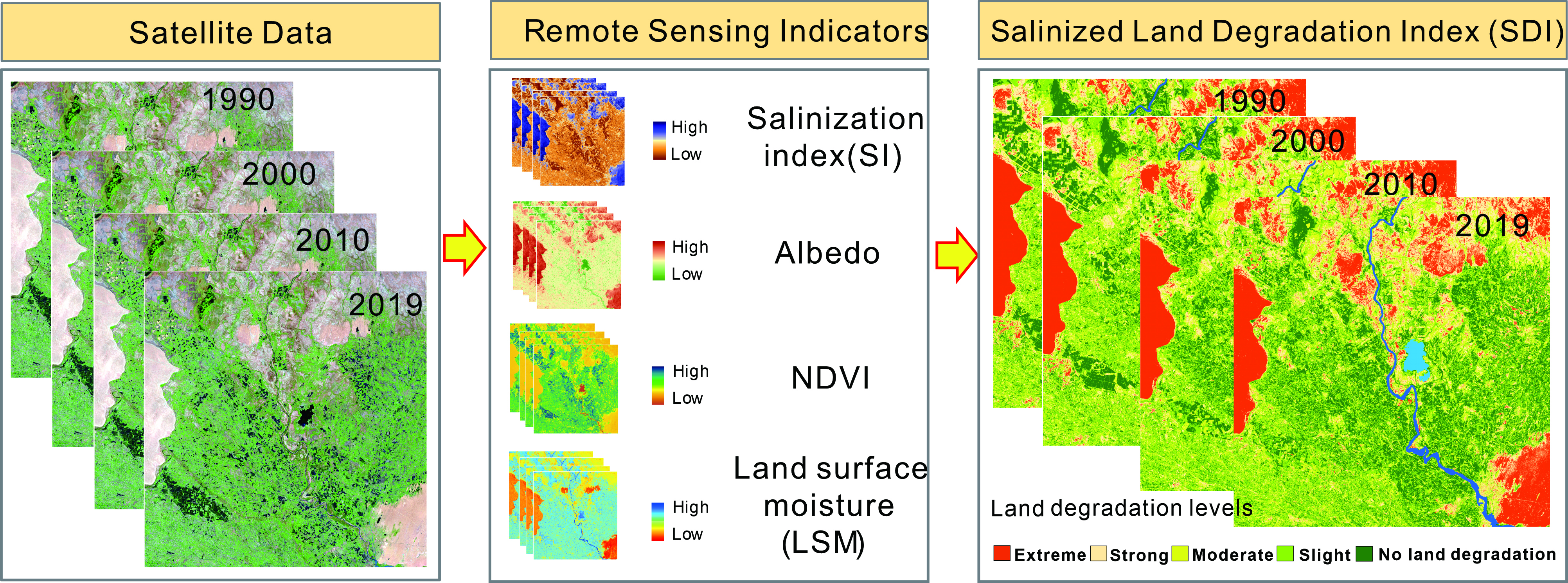
2.1. Study Area

The ADD is located south of the Aral Sea, downstream of the Amu Darya River (Figure 1). The region runs through Turkmenistan and Uzbekistan and covers an area of 6.3 × 10⁴ km². The runoff from large permanent glaciers in the mountains and melting snow are the main water sources of the Amu Darya River [37]. The ADD has a typical continental climate characterised by extreme dryness throughout the year. The average annual temperature is approximately 13 °C [37]. The potential annual evapotranspiration can be as high as 1600 mm, and the average annual precipitation is less than 100 mm [37]. Such a dry climate makes the ADD one of the most ecologically fragile regions worldwide [9].

However, as the main grain-producing region of the Aral Sea basin, dry climate and land use changes due to agricultural expansion have further exacerbated the salinization of the ADD [38]. Moreover, the changes in the political system after the disintegration of the Soviet Union have led to intensified conflicts in the use of water resources among different countries in the region, resulting in land degradation and a decline in the stability of the ecological system [39]. In this regard, a series of ecological conservation and restoration projects have been implemented or are about to be launched to mitigate the land degradation caused by salinization of the ADD [40]. Within this context, it is essential to investigate the spatial and temporal characteristics of the land degradation in the ADD, a typical salinized region, to provide reference for the ecosystem management of the delta.

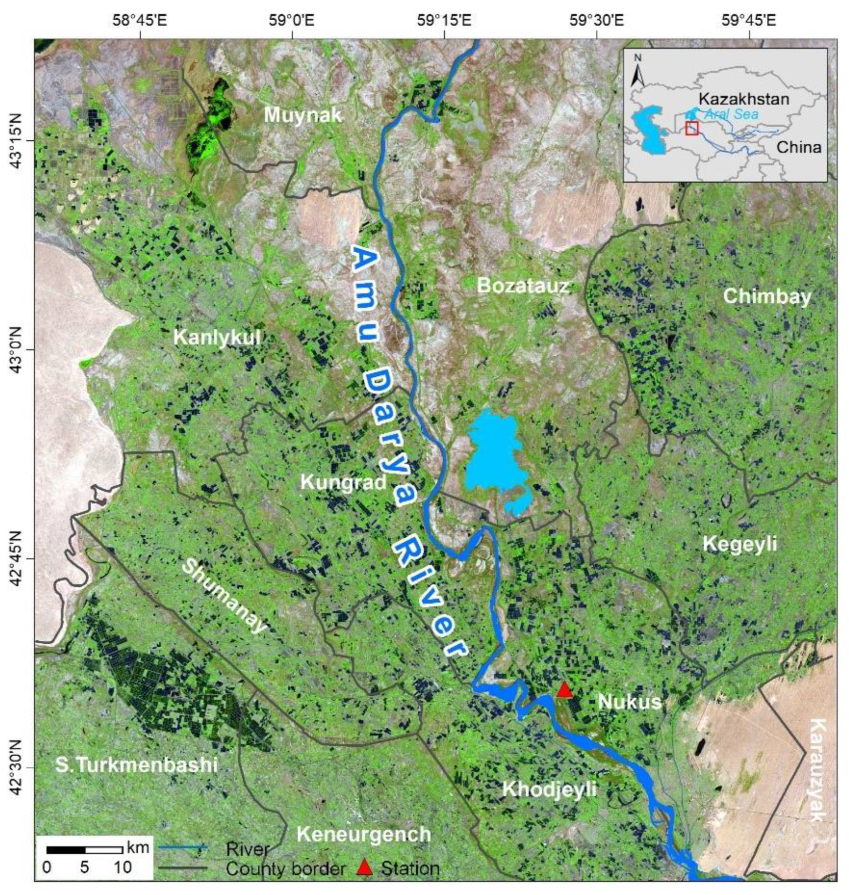
2.2. Data and Pre-Processing

The datasets used in this study included satellite images, field soil salinity, temperature and precipitation, land use and water withdrawal and salt discharge data. The satellite images from the United States Geological Survey (http://earthexplorer.usgs.gov/, accessed on 5 June 2020), acquired on 19 July and 26 July 1990, July 21 and 30 July 2000, 10 July and 17 July 2010 (Landsat-5 TM) and 4 August and 11 August 2019 (Landsat-8 OLI/TIRS) were used. The selected images were in the growing season, and the time phase was similar, and there was basically no cloud coverage, which ensured the accuracy of the remote sensing index calculations [41,42]. The images were first radiometrically corrected with ENVI 5.1 software to convert the digital numbers to irradiance values and later atmospherically corrected using the Fast Line-of-sight Atmospheric Analysis of Spectral Hypercubes (FLAASH) module to eliminate the effects of noise generated during the imaging process [43,44]. The images acquired at different times were geometrically corrected using the two polynomials, and the root mean square error was controlled within 0.5 pixels [33]. Finally, the images were clipped based on the ADD boundary, and the water bodies were masked using the modified normalised difference water index (MNDWI) [45].

The salinity data sampled in the field on 18 March 2019 (see Figure S1 and Table S1 for details) were used to explore the feasibility of the SDI in assessing the land degradation in salinized areas. The average annual precipitation and temperature records during 1980–2016 were derived from Nukus Station in the ADD. The annual statistical data on water withdrawal and salt discharge data for 1990–2015 were obtained from the Amu Darya River basin database of the Inter-State Commission for Water Coordination of Central Asia (ICWC, http://www.cawaterinfo.net/, accessed on 10 June 2020). The land use data were obtained from the Xinjiang Institute of Ecology and Geography, Chinese Academy of Sciences and interpreted based on the Landsat images from 1990, 2000, 2010 and 2019 that have been applied in related studies in the ADD [10,46]. Following this dataset, the land use types were divided into five categories: cropland, forest, grassland, built-up land and bare soil.

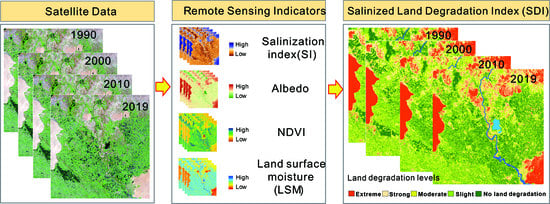
2.3. Construction of the SDI

2.3.1. SI

Salinization is the major factor influencing the land degradation of the ADD. The SI extracted from the remote sensing image has been shown to be able to assess the characteristics of regional salinization [47,48,49]. In this work, an inversion model that has been proved to be applicable in the ADD [10,50] was selected to construct the SI. The model was derived using the following equation [20]:

$$\mathrm{S}\mathrm{I}=\sqrt{{\rho }_{\mathrm{B}\mathrm{l}\mathrm{u}\mathrm{e}}\times {\rho }_{\mathrm{R}\mathrm{e}\mathrm{d}}}$$

(1)

where ρBlue and ρRed are the blue and red bands of the Landsat TM and OLI imagery, respectively.

2.3.2. Albedo

The albedo is a key physical parameter related to the soil exposure [51]. In general, the albedo is higher in desert areas due to the sparse vegetation and soil exposure, and areas with high vegetation cover exhibit a lower albedo [23,52]. Therefore, the albedo was chosen to represent the surface exposure, and it was calculated as follows [51]:

$$\begin{array}{l}\mathrm{A}\mathrm{l}\mathrm{b}\mathrm{e}\mathrm{d}\mathrm{o}=0.356{\rho }_{\mathrm{B}\mathrm{l}\mathrm{u}\mathrm{e}}+0.130{\rho }_{\mathrm{R}\mathrm{e}\mathrm{d}}+0.373{\rho }_{\mathrm{N}\mathrm{I}\mathrm{R}}+0.085{\rho }_{\mathrm{S}\mathrm{W}\mathrm{I}\mathrm{R}\mathrm{1}}\\ +0.072{\rho }_{\mathrm{S}\mathrm{W}\mathrm{I}\mathrm{R}2}-0.018\end{array}$$

(2)

where ρBlue, ρRed, ρNIR, ρSWIR1 and ρSWIR2 denote the blue, red, near-infrared and two shortwave-infrared bands of the Landsat TM and OLI imagery, respectively. These bands are the same as those referred to in the following text.

2.3.3. NDVI

The NDVI is based on the structure absorbed by the plant leaf surface that reflects the parameters of the plant biomass and vegetation coverage [53]. This parameter has been successfully used to monitor land degradation at different scales [54], and its expression is as follows:

$$\mathrm{N}\mathrm{D}\mathrm{V}\mathrm{I}=({\rho }_{\mathrm{N}\mathrm{I}\mathrm{R}}–{\rho }_{\mathrm{R}\mathrm{e}\mathrm{d}})/({\rho }_{\mathrm{N}\mathrm{I}\mathrm{R}}+{\rho }_{\mathrm{R}\mathrm{e}\mathrm{d}})$$

(3)

2.3.4. LSM

The LSM is crucial to regulate the vegetation productivity, and it directly affects the regional land degradation [55]. The LSM can be calculated using the tasselled cap transformation through the following formulas [56,57]:

$$\begin{array}{l}\mathrm{L}\mathrm{S}{\mathrm{M}}_{\mathrm{T}\mathrm{M}}=0.0315{\rho }_{\mathrm{B}\mathrm{l}\mathrm{u}\mathrm{e}}+0.2021{\rho }_{\mathrm{G}\mathrm{r}\mathrm{e}\mathrm{e}\mathrm{n}}+0.3102{\rho }_{\mathrm{R}\mathrm{e}\mathrm{d}}+0.1594{\rho }_{\mathrm{N}\mathrm{I}\mathrm{R}}\\ –0.6806{\rho }_{\mathrm{S}\mathrm{W}\mathrm{I}\mathrm{R}1}–0.6109{\rho }_{\mathrm{S}\mathrm{W}\mathrm{I}\mathrm{R}2}\end{array}$$

(4)

$$\begin{array}{l}\mathrm{L}\mathrm{S}{\mathrm{M}}_{\mathrm{O}\mathrm{L}\mathrm{I}}=0.1511{\rho }_{\mathrm{B}\mathrm{l}\mathrm{u}\mathrm{e}}+0.1972{\rho }_{\mathrm{G}\mathrm{r}\mathrm{e}\mathrm{e}\mathrm{n}}+0.3283{\rho }_{\mathrm{R}\mathrm{e}\mathrm{d}}+0.3407{\rho }_{\mathrm{N}\mathrm{I}\mathrm{R}}\\ –0.7117{\rho }_{\mathrm{S}\mathrm{W}\mathrm{I}\mathrm{R}1}–0.4559{\rho }_{\mathrm{S}\mathrm{W}\mathrm{I}\mathrm{R}2}\end{array}$$

(5)

where ρ denotes the corresponding bands of the Landsat TM and OLI imagery.

2.3.5. Constructing SDI Based on PCA

In this study, based on previous studies [33,58,59], the PCA method was used to synthesize the four selected indicators (SI, albedo, NDVI and LSM) to construct the SDI. Before using the PCA method to couple the SDI for 1990, 2000, 2010 and 2019, respectively, it is necessary to normalise the four indicators in the range of 0 to 1 [58] by Equation (6). The SDI obtained using Equation (7) and higher values of the SDI revealed more severe land degradation. Figure 2 illustrates the processing for SDI.

$$I_{normal}=(\mathrm{I}-{\mathrm{I}}_{\min })/({\mathrm{I}}_{\max }-{\mathrm{I}}_{\min })$$

(6)

$$\mathrm{S}\mathrm{D}\mathrm{I}=\mathrm{P}\mathrm{C}1\left[\mathrm{f}(\mathrm{S}\mathrm{I},\mathrm{A}\mathrm{l}\mathrm{b}\mathrm{e}\mathrm{d}\mathrm{o},\mathrm{N}\mathrm{D}\mathrm{V}\mathrm{I},\mathrm{L}\mathrm{S}\mathrm{M})\right]$$

(7)

where I_noraml is the index value after standardisation, I is the numerical value of this index, and I_max and I_min are the maximum and minimum values of the relevant index, respectively.

2.4. Spatial Autocorrelation Analysis

A spatial autocorrelation analysis is an effective way to test whether the values of adjacent samples of a spatial variable are correlated [60]. In this study, the global Moran’s I index and the local indicator of spatial association (LISA) were used to analyse the spatial correlation of the SDI.

Moran’s I generates a global assessment for spatial autocorrelation, with Moran’s I values ranging from −1 to 1 [61,62]. Moran’s I value > 0 means that the SDI has a positive spatial autocorrelation, while Moran’s I value < 0 means that the SDI has a negative spatial autocorrelation. The closer the value to 1, the stronger the positive spatial autocorrelation, and the closer the value to −1, the stronger the negative spatial autocorrelation. Moran’s I = 0 means that there is no spatial autocorrelation, and the SDI has a random spatial distribution. The global Moran’s I index was calculated using the following equations:

$$\mathrm{I}=\frac{{\sum }_{\mathrm{i}}^{\mathrm{n}}{\sum }_{\mathrm{j}\ne \mathrm{i}}^{\mathrm{n}}{\mathrm{W}}_{\mathrm{i}\mathrm{j}}({\mathrm{x}}_{\mathrm{i}}-\overline{\mathrm{x}})({\mathrm{x}}_{\mathrm{j}}-\overline{\mathrm{x}})}{{\mathrm{S}}^2{\sum }_{\mathrm{i}}^{\mathrm{n}}{\sum }_{\mathrm{j}\ne \mathrm{i}}^{\mathrm{n}}{\mathrm{W}}_{\mathrm{i}\mathrm{j}}}$$

(8)

$${\mathrm{S}}^2=\frac{1}{\mathrm{n}}\sum _{\mathrm{i}}^{\mathrm{n}}{({\mathrm{x}}_{\mathrm{i}}-\overline{\mathrm{x}})}^2$$

(9)

$$\overline{\mathrm{x}}=\frac{1}{\mathrm{n}}\sum _{\mathrm{i}(\mathrm{j})}^{\mathrm{n}}{\mathrm{x}}_{\mathrm{i}(\mathrm{j})}$$

(10)

$${\mathrm{Z}}_{\mathrm{S}\mathrm{c}\mathrm{o}\mathrm{r}\mathrm{e}}=\frac{1-\mathrm{E}(\mathrm{I})}{\sqrt{\mathrm{V}\mathrm{a}\mathrm{r}(\mathrm{I})}}$$

(11)

where x_i and x_j are the values of the SDI at spatial locations i and j, respectively, x is the mean value of the SDI, S² is the mean squared deviation of the SDI, W_ij is the spatial weight value, which is expressed by the n-dimensional matrix W(n×n), var(I) is the variance of Moran’s I, and E(I) is the expected value of Moran’s I.

LISA is a local statistical method for spatial variables that reveals the spatial clustering characteristics of observations within spatially adjacent regions [33,60]. A positive LISA value indicates that the SDI is similar to the adjacent value and reveals a spatial pattern of high–high clustering (H–H, high values are near other high values) or low–low clustering (L–L, low values are near other low values). A negative LISA value indicates that the SDI is a spatial outlier and can include a high–low outlier value (H–L, a high value is near a low value) and a low–high outlier value (L–H, a low value is near a high value).

3. Results

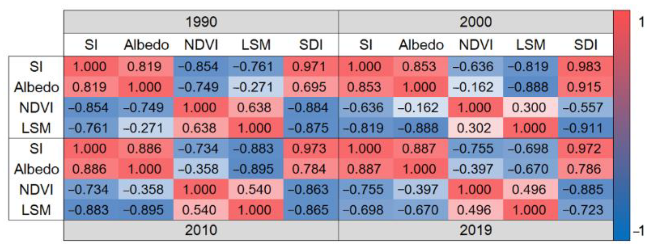
3.1. Integration of the Remote Sensing Indexes Based on PCA

The SDI of the ADD was calculated by the PC1 of the four indicators. The PC1 results shown in

Table 1. Loadings of the four selected variables on the first principal component (PC1) and associated contributions in different study years.

	1990	2000	2010	2019
Loading of the SI	0.58	0.64	0.57	0.61
Loading of albedo	0.23	0.43	0.23	0.26
Loading of the NDVI	–0.32	–0.16	–0.46	–0.24
Loading of LSM	–0.71	–0.62	–0.64	–0.71
Eigenvalue contribution percentage (%)	78.61	83.24	86.35	87.67

SI: salinization index (SI); NDVI: normalised difference vegetation index; LSM: land surface soil moisture index.

indicated that, during the studied years, the percent eigenvalues of PC1 were higher than 78%, revealing that PC1 integrated most of the information of the four indictors. Therefore, PC1 was chosen to construct the SDI in this study. The loading values of the four variables in PC1 were divided into two types according to their signs. The albedo and SI comprised one type with loading values that were positive, and the NDVI and LSM comprised the second type with loading values that were negative. The opposite signs of the two variables indicated that the corresponding contributions to the SDI value were opposing.

The descriptive statistics of the PC1 indicated that the average PC1 value increased from 0.42 in 2010 to 0.43 in 2000, and the medium value of PC1 also increased from 0.38 to 0.40 (

Table 2. Description statistics of PC1.

	Minimum	Maximum	Mean	Median	Skewness	Kurtosis	Standard Deviation
1990	0.04	1.15	0.42	0.38	0.48	−0.33	0.19
2000	0.04	1.21	0.43	0.40	0.31	0.14	0.16
2010	0.03	1.12	0.41	0.38	0.49	−0.71	0.18
2019	0.04	1.12	0.30	0.28	0.42	−0.80	0.18

). From 2010 to 2019, on the contrary, the average PC1 value decreased from 0.41 to 0.30, and the medium value of PC1 also decreased from 0.38 to 0.28. The positive skewness in 1990, 2000, 2010 and 2019 indicated that the tail on the right side of the probability density function was longer or fatter than the left side. Overall, the statistical results of PC1 showed that land degradation accelerated from 1990 to 2000 and weakened from 2010 to 2019.

Furthermore, the correlation coefficient between each indicator and the SDI and that among the indicators are shown in Figure 3 (at the 0.01 level of significance). For four years, the SDI exhibited a high correlation with each single indicator. In general, the SDI exhibited a positive correlation with the SI and albedo and a negative correlation with the NDVI and LSM (Figure 3). The SI exhibited the highest correlation with the SDI, and the positive correlations were 0.971, 0.983, 0.973 and 0.972 in 1990, 2000, 2010 and 2019, respectively. The albedo exhibited the highest negative correlation with the SDI in 2000, and the correlation was 0.915. The NDVI exhibited the highest correlation with the SDI in 2019 (−0.885). The correlation coefficients between the LSM and SDI were greater than −0.72, and the highest correlation with the SDI was observed in 2000 (−0.911).

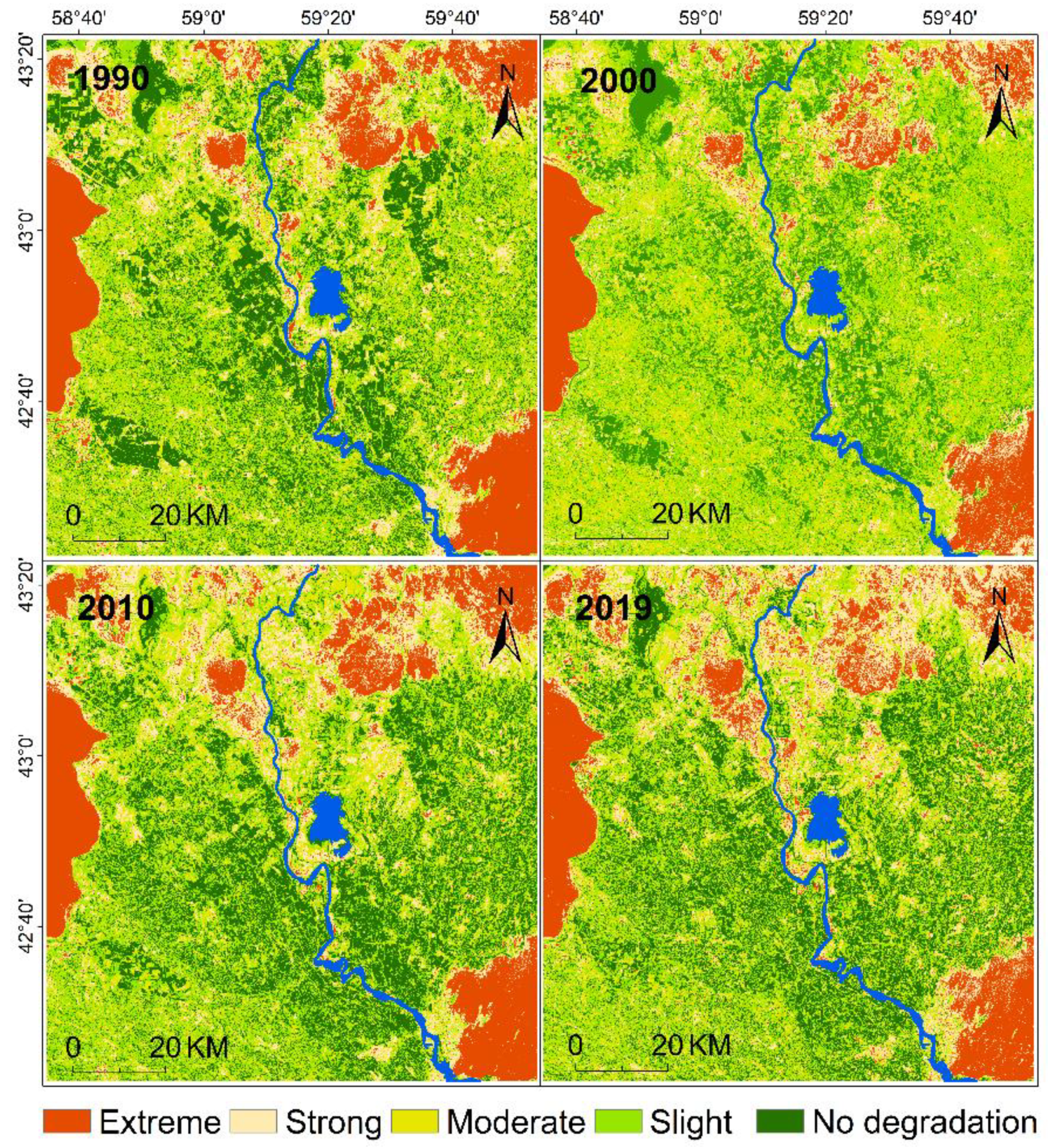
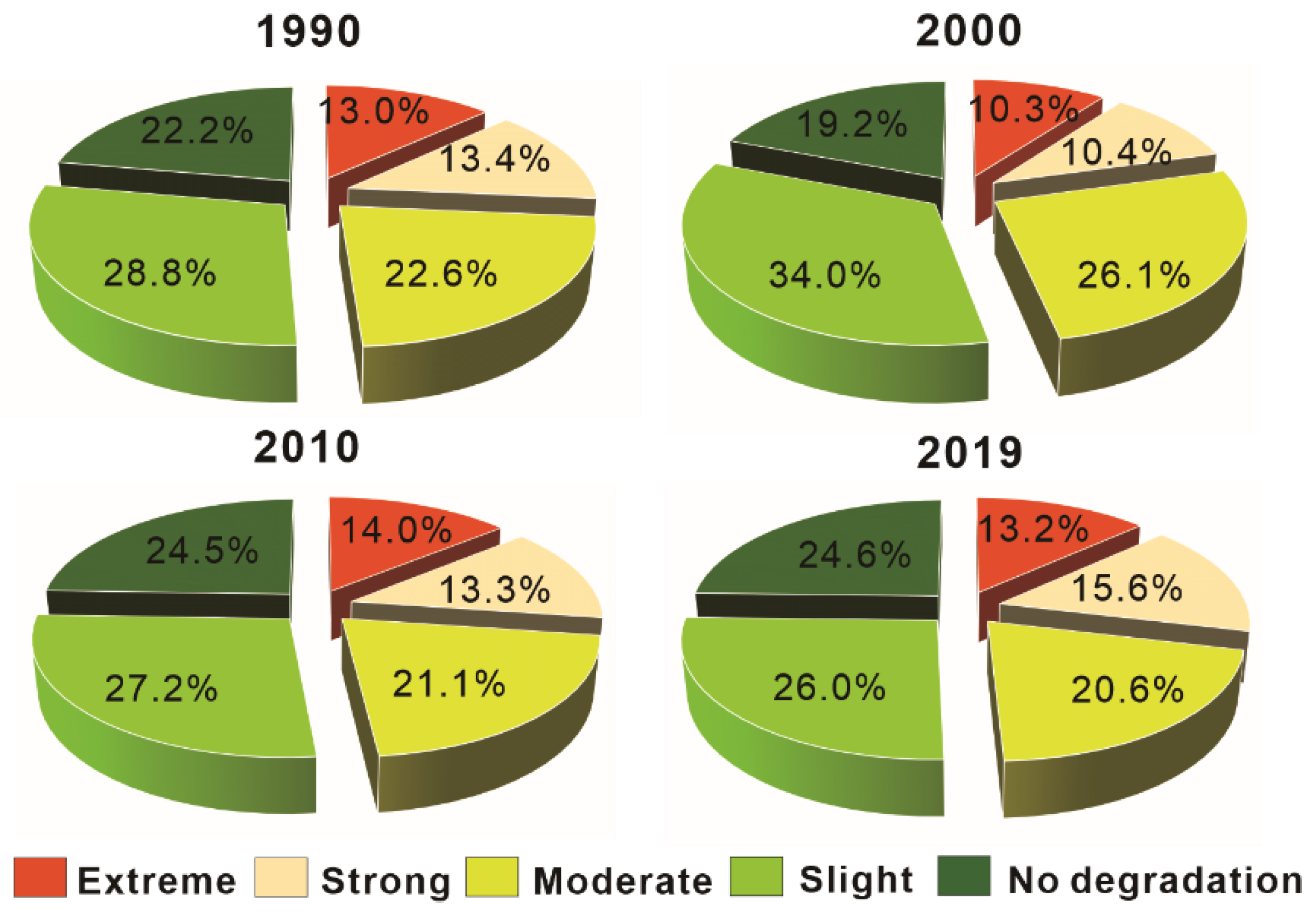
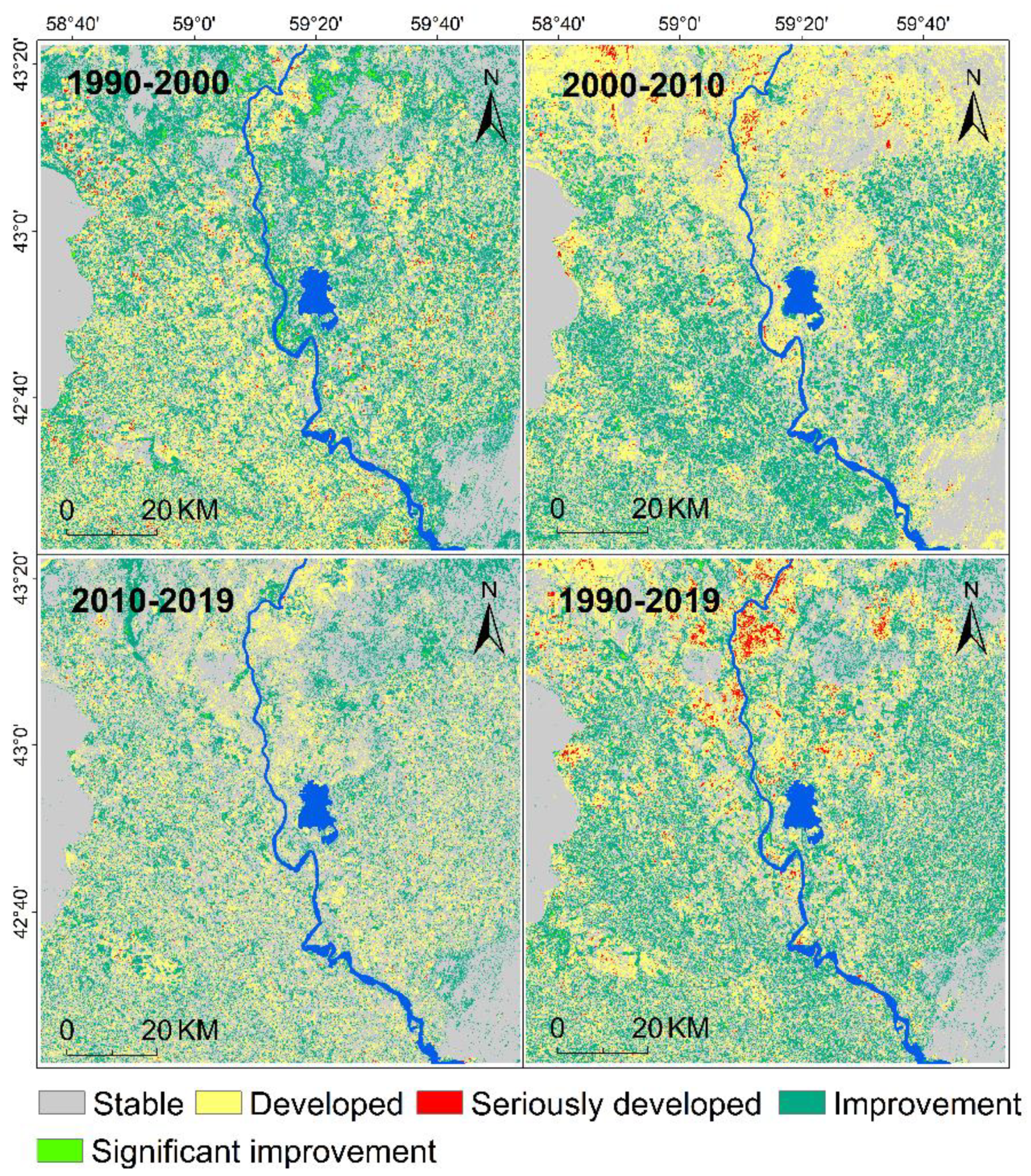
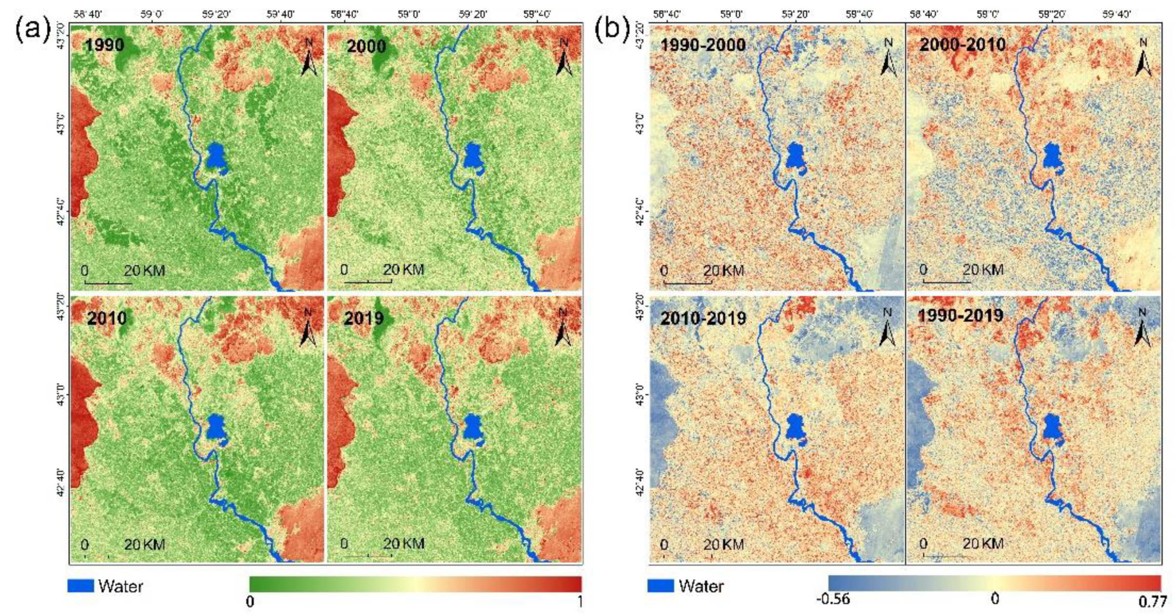
3.2. Spatiotemporal Changes in the Land Degradation

To analyse the spatiotemporal characteristics of the land degradation during the different periods in the ADD, the SDI values were normalised by Equation (6) (range of 0 to 1). As the SDI approximates a normal distribution, we divided it into five categories by equal intervals to indicate the different land degradation levels [36,58]—namely, no degradation (0–0.2), slight degradation (0.20–0.4), moderate degradation (0.4–0.6), strong degradation (0.6–0.8) and extreme degradation (0.8–1). In summary, the land degradation level distribution was not uniform in space and varied over space and time. As shown in Figure 4, in terms of the land degradation level distribution, the extreme and strong degradation areas were clustered in the west and north of the ADD during the studied years. Areas with moderate degradation corresponded to a sporadic distribution in the middle and south of the ADD. Most areas in the middle of the ADD exhibited a slight degradation. The spatial distribution of the not-degraded areas in the study area showed a difference in the 4 years: in 1990 and 2000, the not-degraded areas were mainly distributed along the Amu Darya River, and a small portion appeared in the northwest and northeast corners of the ADD; in contrast, the not-degraded areas were mainly distributed in the middle of the study area in 2010 and 2019 and formed a “V” shape.

Figure 5 shows the percentage of the study area occupied by the five land degradation levels in 1990, 2000, 2010 and 2019. In general, the largest areas in the ADD were slight degradations in the years 1990–2019, which accounted for more than 26% of the total area covered by the Landsat images. From 1990 to 2000, the areas with extreme, strong and no degradation decreased, whereas the areas with slight and moderate degradations increased. From 2000 to 2010, the areas with extreme, strong and no degradation expanded; among which, the expansion of the no degradation regions was significant. In contrast, the areas with slight and moderate degradations exhibited a decreasing trend; in particular, for the areas with a slight degradation, the dynamic degree was 7%. From 2010 to 2019, a small increase from 13.30% to 15.56% of the total area was observed in the area with moderate degradation, and the areas of the other four levels did not change considerably.

Using a spatial analysis, the land degradation spatial distribution changes from 1990 to 2000, 2000 to 2010, 2010 to 2019 and 1990 to 2019 were mapped (Figure 6). We defined the figure elements as follows: development of land degradation across levels 1 or 2 corresponded to “Developed” (e.g., a change from “No degradation” to “Slight degradation” or “Moderate degradation”), a development across levels 3 or 4 corresponded to “Seriously developed” (e.g., a change from “No degradation” to “Strong degradation” or “Extreme degradation”), an improvement of the land degradation across levels 1 or 2 corresponded to “Improvement” (e.g., a change from “Extreme degradation” to “Strong degradation” or “Moderate degradation”), an improvement across levels 3 or 4 corresponded to “Significant improvement” (e.g., a change from “Extreme degradation” to “Slight degradation” or “No degradation”), and no change during the study periods corresponded to “Stable”. The areas of land degradation dynamics for the four periods are shown in

Table 3. Area and proportion of land degradation developed or an improvement of the ADD during different time periods.

Type	1990–2000		2000–2010		2010–2019		1990–2019
	km2	%	km2	%	km2	%	km2	%
Seriously developed	130.0	1.1	110.1	0.9	40.3	0.3	217.8	1.8
Developed	2687.5	22.5	3728.8	31.3	2438.0	20.5	2901.7	24.3
Stable	5291.8	44.4	5094.0	42.7	7061.7	59.2	5385.8	45.2
Improvement	3653.8	30.6	2886.0	24.2	2354.3	19.7	3314.7	27.8
Significant improvement	160.5	1.4	104.8	0.8	29.8	0.3	103.4	0.9

.

Overall, the stable areas accounted for a large proportion (more than 42%) during the four study periods (Table 3), and these areas were mainly located west and southeast of the ADD. From 1990 to 2000, the improvement areas covered 3653.78 km² (30.6%), and these areas were mainly clustered north of the ADD (Figure 6). Additionally, the developed areas covered 2687.53 km² (22.5%), and these areas mainly occupied the south and middle regions of the ADD. A smaller proportion (1.4%) of significant improvement areas was observed in the northern part of the ADD. In comparison, the proportion of the seriously developed areas was smaller (1.1%), and these areas were mainly located in the northwest corner of the ADD. From 2000 to 2010, the developed areas covered 3728.76 km² (31.3%), and the areas were mainly concentrated in the northern part of the study area. The improvement areas covered 2886.02 km² (24.2%) from 2000 to 2010 and were mainly located in the eastern and central parts of the ADD. The areas of seriously developed and significant improvement exhibited smaller proportions—0.92% and 0.88%, respectively—and the seriously developed areas were mainly observed downstream of the ADD. Compared with those in 2000–2010, during 2010–2019, the areas with developed, and the improvements exhibited decreasing trends and occupied 20.5% and 19.7% of the total area, respectively. Moreover, these regions were mainly clustered in the downstream of the ADD. The seriously developed and significant improvement areas occupied less than 0.4% of the total area. From 1990 to 2019, the developed areas covered 2901.65 km² (24.3%) and were mainly concentrated north of the ADD and in the downstream region of the Amu Darya River. The improvement regions, which occupied 27.8% of the total area, were mainly observed in the west and east of the ADD. The seriously developed regions, with an area of approximately 217.75 km², were mainly concentrated in the north of the ADD, and the areas with significant improvement were smaller, accounting for only 0.9% of the total area.

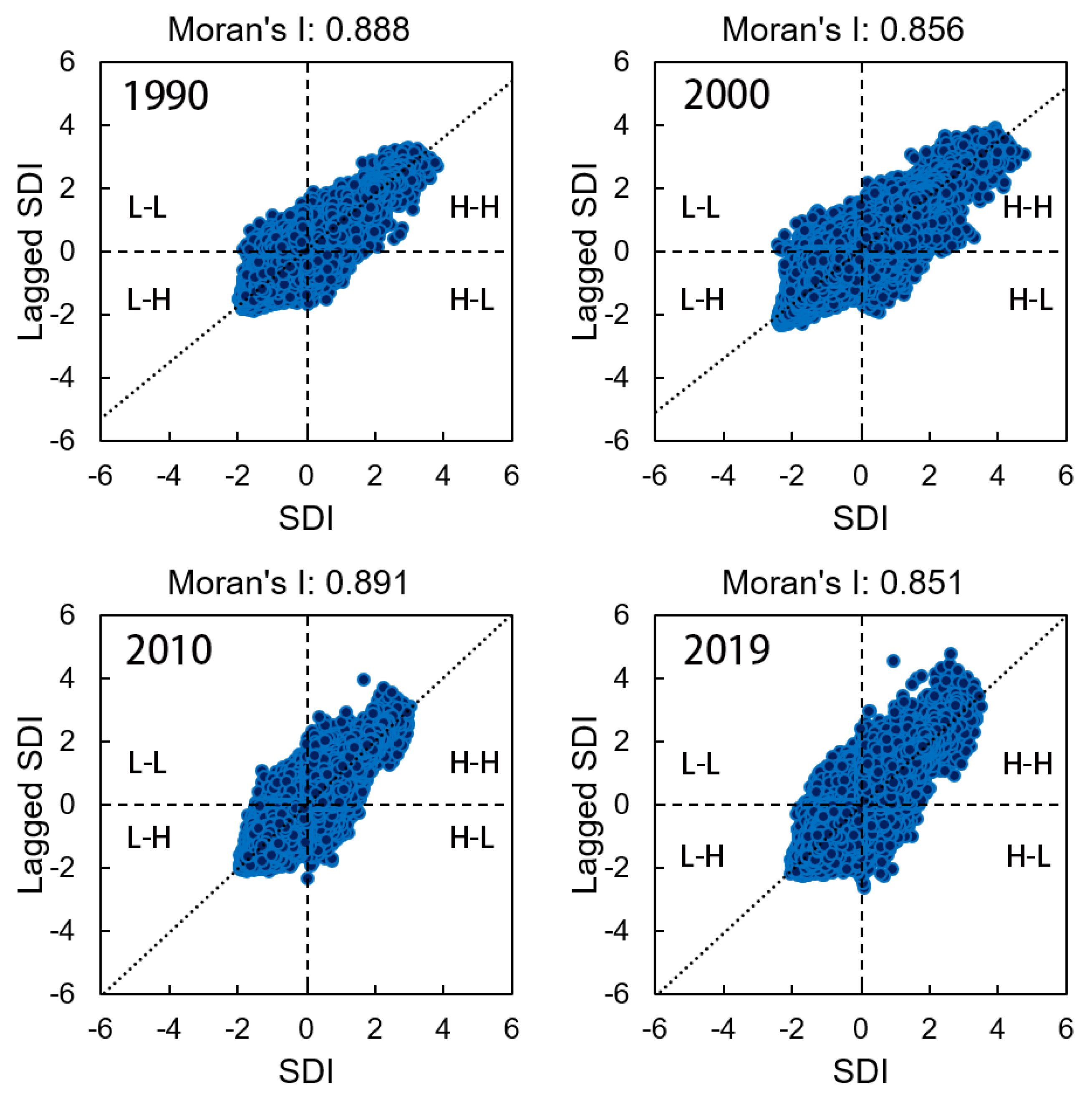
3.3. Spatial Autocorrelation Analysis of the SDI

To further clarify the spatial and temporal variabilities in the land degradation, the spatial autocorrelation of the SDI was examined.

The mapping of the global spatial autocorrelation of the SDI is shown in Figure 7. Most of the SDI values are distributed in the first and third quadrants, with H–H and L–L clustered in the first and third quadrants, respectively, indicating a strong positive spatial correlation between the spatial units in these two quadrants. The Moran’s I values in 1990, 2000, 2010 and 2019 were 0.888, 0.856, 0.891 and 0.851, respectively, which were high values greater than zero. The results showed that the SDI of the ADD exhibited significant spatial clustering, which indicated a strong positive spatial correlation. The Moran’s I values of the SDI decreased, increased and later decreased again in 1990, 2000, 2010 and 2019, exhibiting an overall decreasing trend during the study period.

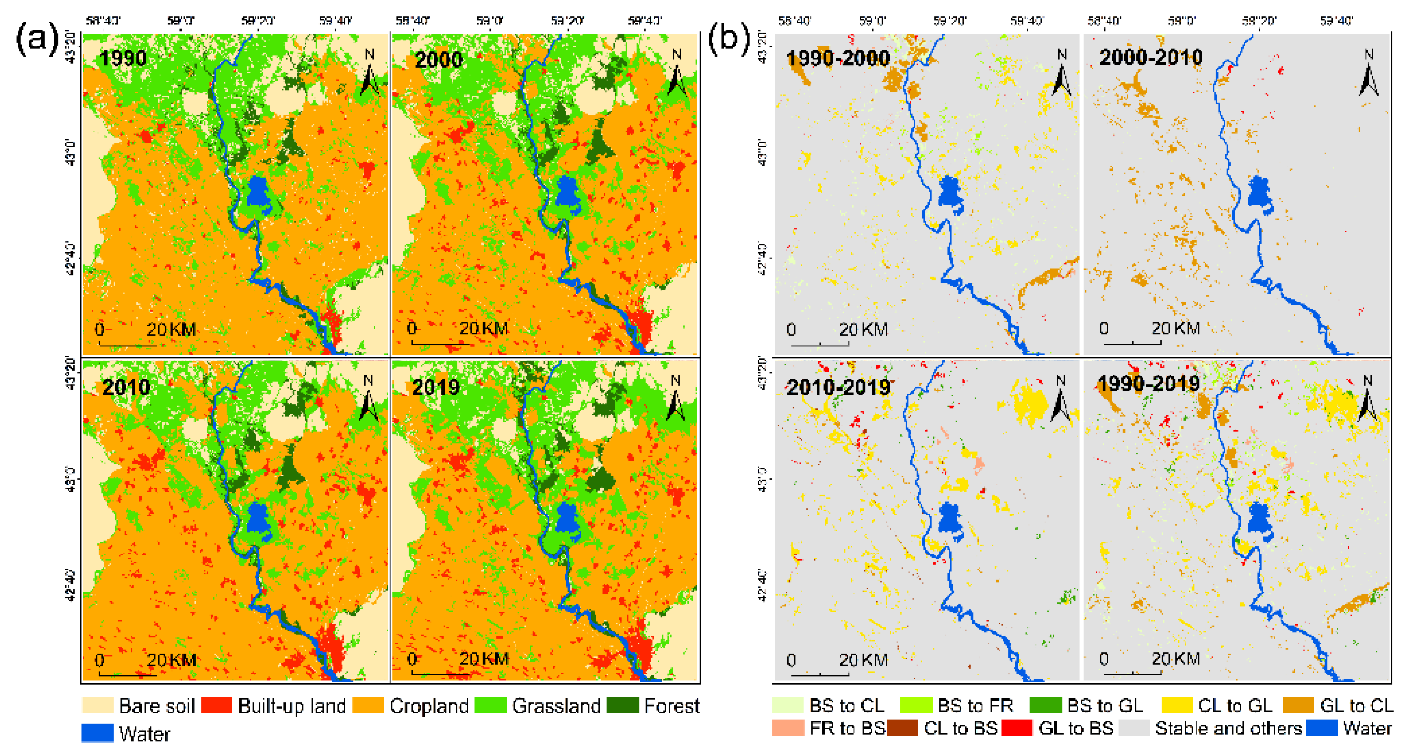
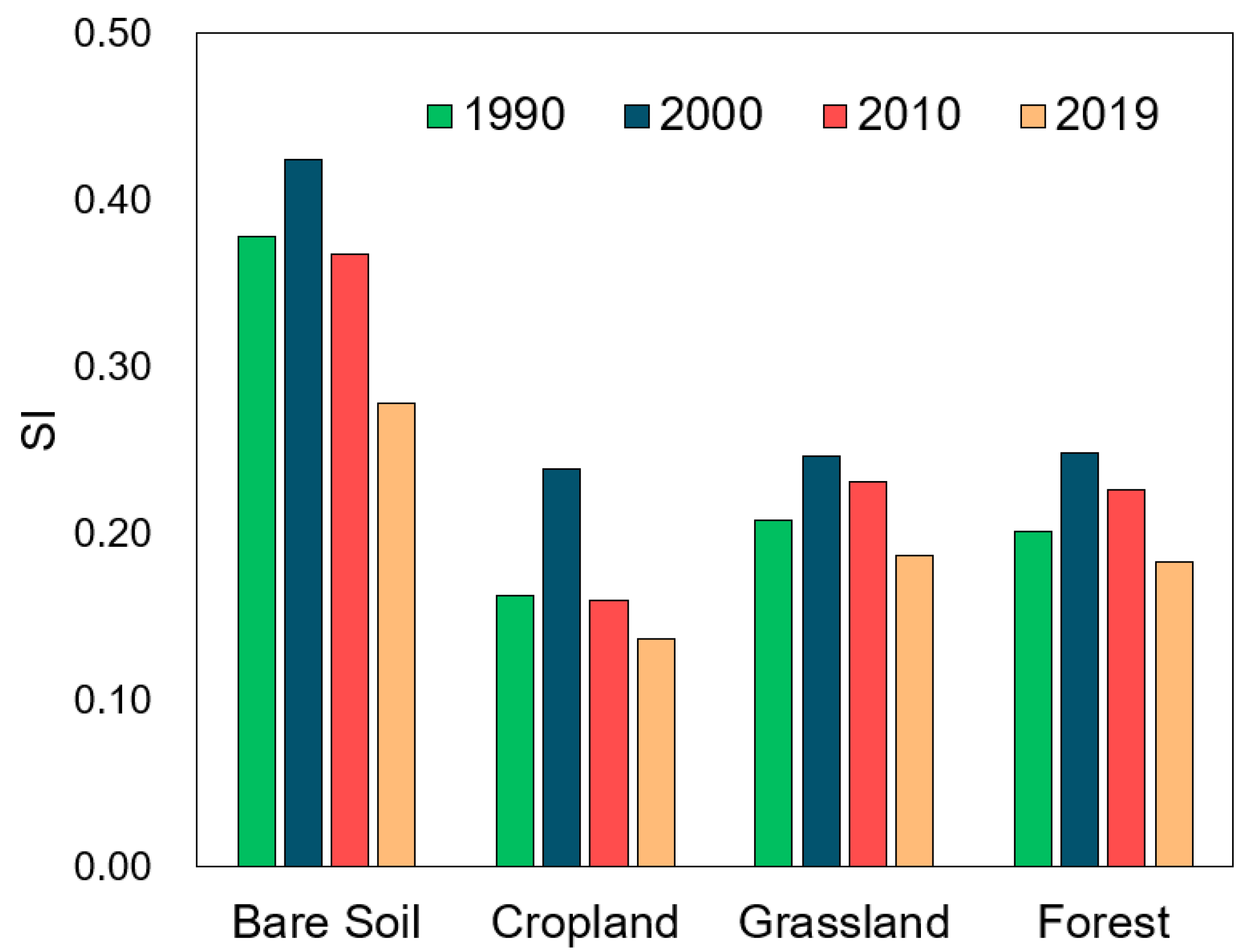
3.4. Spatial and Temporal Changes in Land Use and Salinization

Figure 8 displays the land use maps for 1990, 2000, 2010 and 2019. These land use maps indicated that croplands were the dominant land use type in the ADD. Grassland and forest were distributed in the north of the ADD and bare soil mainly in the edge and north of the ADD. Figure 8b displays the spatial variations in the land use types. The combinations with no land use type transformations, smaller conversion areas and built-up land transformations were merged into “Stable and others”. From 1990 to 2010, the conversion of land use categories was mainly between grasslands and croplands. The conversion from grassland to cropland (GL to CL) was prominent in the northern part of the ADD, where the area of grassland decreased by 158.74 km² and 338.93 km² from 1990 to 2000 and 2000 to 2010, respectively (

Table 4. Areas and percentages of different land use types from 1990 to 2019 in the ADD.

	1990		2000		2010		2019
Type	km2	%	km2	%	km2	%	km2	%
Bare soil	2165.71	18.42	1968.62	16.74	1946.80	16.56	1989.45	16.92
built-up land	205.52	1.75	528.64	4.50	570.81	4.85	588.47	5.00
Cropland	6593.86	56.08	6624.91	56.34	6952.42	59.13	6350.16	54.01
Grassland	2412.67	20.52	2253.93	19.17	1915.46	16.29	2407.83	20.48
Forest	380.66	3.24	382.32	3.25	372.93	3.17	422.51	3.59

). However, the conversion of land use categories from 2010 to 2019 was mainly cropland to grassland (CL to GL), which was distributed in the northern and western parts of the ADD. The area of cropland decreased by 602.26 km², and the area of grassland increased by 492.37 km² during this period. In addition, there was partial degradation of grassland to bare soil (GL to BS) in the northern part of the ADD from 2010 to 2019. The conversion of land use categories throughout the study period was mainly from grassland to cropland and cropland to grassland.

Figure 9 reveals the spatial distribution (Figure 9a) and variation (Figure 9b) of the SI over the study time period. The values of the SI were larger at the edges and north of the ADD and smaller in the centre. The SI in the northern part of the ADD decreased from 1990 to 2000, while it increased significantly from 2000 to 2010. From 2010 to 2019, the SI increased slightly in the central part of the ADD and decreased in the northeast. Throughout the study period (1990–2019), the SI increased significantly in the northern part of the ADD and decreased at the edges. To reveal the relationship between land use change and salinization, the mean SI values for each land use type (built-up land and water were excluded) were calculated in Figure 10. The mean value of the SI for the land use type was the largest in 2000 compared to the other three years, indicating higher soil salinization. The mean value of the SI for the land use type was the largest in 2000 compared to the other three years, indicating higher soil salinization, with a decreasing trend in the SI from 2000 to 2019. Within each year, bare soil had the largest mean value of the SI, followed by grassland and forest.

The dynamic characteristics of salinization during land use change were illustrated in Figure 11. The ΔSI represents the difference in the SI over the study period (the following year minus the previous year). We counted a percentage of areas with ΔSI < 0 and ΔSI < 0 over the course of each land use type transfer. The SI increased during all land use type changes from 1990 to 2000 (more than 50% of the area with ΔSI > 0), which was related to the maximum SI value in 2000 mentioned earlier. The 2000–2010 SI values decreased for BS-CL and GL-CL (ΔSI < 0 over 80% of the area). The area with ΔSI < 0 dominated the land use change process from 2010 to 2019. During the conversion of bare soil to cropland (BS-CL), forest (BS-FR) and grassland (BS-GL) from 1990 to 2019, the area with ΔSI < 0 exceeded 50%, indicating a decrease in the SI.

4. Discussion

4.1. Effectiveness of the Proposed SDI

In this study, we established a new SDI by integrating the SI, albedo, NDVI and LSM indices based on the PCA method. The SDI was used to explore the land degradation characteristics for a typical salinized area, i.e., the ADD. We found that the regions with extreme land degradation were mainly distributed downstream and at the periphery of the ADD (Figure 4). The SDI-based results supported previous findings that the ecological risks and vulnerabilities are higher in the downstream and peripheral regions of the ADD [10,46], thereby demonstrating that the SDI can reflect the land degradation conditions of the ADD. To further evaluate the effectiveness of the proposed SDI, we evaluated its effectiveness by field survey data (Figure S1 and Table S1). The relationship between the SDI and soil salt content shown in Figure 12 indicates that the soil salt content was significantly positively correlated with the SDI (R² = 0.89, p < 0.001). The relationships between the four indices derived from Landsat imagery in 2019 and field-measured soil salinity are also presented in Figure S2. There was a positive correlation between the SI, albedo and measured soil salinity (R² = 0.41 and 0.43, respectively) and a negative correlation between the NDVI, LSM and measured soil salinity (R² = 0.29 and 0.19, respectively). In contrast to the single indices, the SDI showed a stronger agreement with the measured soil salinity. In general, although the land degradation is influenced by multiple aspects of the environment, this positive correlation suggests that the SDI can capture the salinity features pertaining to the land degradation, which provides potential evidence for the effectiveness of the index in monitoring the land degradation in salinized areas. In addition, the SI extracted from the remote sensing data exhibits a positive correlation with the SDI (Figure 3). The reliability of the SDI is also reflected in the other three indicators. High vegetation cover and sufficient soil moisture reduce the risk of land degradation, and this finding is supported by the negative correlation between the SDI and NDVI and LSM in our study (Figure 3). An increase in the albedo values leads to a higher SDI, which is related to the exposure information represented by the albedo and may be attributed to a strong coupling between the soil salinity information and albedo (Table 1 and Figure 3). These characteristics have also been reported previously [33]. These results indicate that the SDI can help reliably and efficiently monitor the land degradation of salinized areas. In addition, the SDI is composed of accessible remote sensing indicators and can thus be extended to other similar ecological environments [35,59,63].

4.2. Factors Influencing the Land Degradation in the ADD

Climate variables mainly affect the land degradation through changes in the precipitation and temperature [10,64]. The annual mean precipitation (AMP) and annual mean temperature (AMT) of Nurkus Weather Station are shown in Figure 13. It can be noted that the AMP decreased and AMT increased in the ADD in the past 40 years. From 1990 to 2019, land degradation developed over an area of more than 3000 km² (Table 3). Previous studies have raised concerns regarding the withering of grasslands and sparse vegetation caused by warming and dry climates in the ADD, warning that these aspects could accelerate land degradation [10,65].

Amu Darya River is the main source of water for ADD living and irrigation. Overwatering has disrupted the water system of the ADD, leading to the disappearance of an amount of lakes, followed by local climate change, which has reduced the ecosystem stability of the ADD, particularly in the downstream region [7,10]. The widespread use of diffuse irrigation has caused individuals to compensate for inefficient irrigation by collecting large amounts of water, resulting in a reduction in the ecological water that sustains the ecosystems and the gradual withering of vegetation without sufficient water to support growth [9,66,67], exacerbating the land degradation. The extent of the land degradation followed the same trend as that of the water withdrawal from Amu Darya River. With the decline in the water withdrawal in 1990–2000 (Figure 14), the improvement in ADD land degradation was most pronounced, while, in 2000–2019, as the water withdrawal increased, the land degradation developed in a larger area than the improvement area. A more critical situation is that the reservoir built in the upper reaches of the Amu Darya River intercepted a large amount of the water [66], resulting in a decrease in the supply of ecological water downstream. The ecological effects caused by these factors were confirmed by our research: The land degradation downstream of the ADD was significantly degraded compared with the region in the study period (Figure 4 and Figure 6). In addition, the higher levels of land degradation in the outer delta, farther from Amu Darya River, were likely caused by the lack of water supply to the ecosystem and the difficulties in the land management in the transboundary area [46,68]. This finding indicates that, to alleviate the ADD land degradation and the ecological crisis in the Aral Sea basin, further effort and cooperation is necessary in the rational allocation of water resources.

In addition, the impacts of land-use changes on the land degradation cannot be ignored [10,69,70]. The consolidation and management of croplands can contribute to the mitigation of land degradation, and our research supports this perspective. We demonstrated that the area with no degradation occupied a larger proportion of cropland during most of the study period, while the area with extreme land degradation was mainly distributed on bare soil (Figure 15). In general, the risk of land degradation was reduced when land with sparse vegetation and bare soil was reclaimed as cropland, as crops contribute to higher ecosystem productivity and stability. Land degradation is more severe in the northern part of the ADD, where part of the cropland has been abandoned and converted into grassland or bare soil (Figure 8). Previous studies have indicated that the ADD is facing an ecological threat posed by the degradation of grasslands and croplands to bare soil [10,46]. Compared to the other land use categories, bare soil has a higher soil salinity (Figure 10), and the conversion of land use types to bare soil not only reduces the biomass but also increases the risk of soil salinization.

However, to reduce the salt content of croplands, a large amount of water is acquired from Amu Darya River to rinse the cropland soil, which further aggravates the water deficit of other ecosystems. In addition, the excess salinity from croplands is discharged by widely distributed channels to the Amu Darya River, as well as to the lakes downstream of the delta, resulting in increased salinity in the river water and a significant accumulation of salinity downstream (Figure 9) [10]. The increase in the discharge was the most significant after 2000 (Figure 14). The extreme land degradation distribution patterns were noted to be clustered downstream of the ADD (Figure 4 and Figure 6). These ecological effects caused by the large accumulation of salt in the downstream region were confirmed by our research. In addition, with the disintegration of the Soviet Union, the socialist economy turned into a market economy, and the gradual influx of the rural population into cities led to certain croplands eventually transforming into unused lands with a low biodiversity [71], thereby accelerating land degradation.

The 15th initiative of the Sustainable Development Goals (SDGs) aims to achieve land degradation neutrality by 2030. To effectively alleviate land degradation of the ADD and promote the further realisation of SDGs, based on the abovementioned factors influencing the SDI, the following corresponding measures and countermeasures are proposed. First, salinization treatment technology should be implemented to alleviate the promotion of land degradation caused by salinity, and reservoirs for storing salt can be built to reduce the ecological pressure caused by the transportation of salt from the alkali drainage canal that discharges into the downstream area of the ADD. Second, a drip irrigation system can be promoted to achieve precision irrigation and enhance the irrigation efficiency to relieve the pressure of water resources required to maintain the stability of the land degradation. Furthermore, farmers are encouraged to maintain the stability and biodiversity of croplands through agricultural subsidy policies. In addition, ecological conservation projects can be considered to mitigate the impacts of climate change on the land degradation.

5. Conclusions

We coupled multiple remote sensing indices (SI, NDVI, albedo and LSM) to construct a new SDI by using the PCA method. The proposed index integrated the soil salinity, soil bareness, soil moisture and vegetation coverage and made it possible to identify the characteristics of the regional land degradation, especially in salinized areas. To test the reliability of the SDI, the index was applied to the typical ADD region to monitor the spatial and temporal dynamics of the land degradation.

The results indicated that the NDVI and LSM adversely influenced the land degradation, while the SI and albedo had positive effects. The SI was strongly positive correlated with the SDI, with an average correlation coefficient of 0.97. Regions with extreme and strong land degradation were mostly clustered west and north of the ADD. The temporal and spatial dynamics of the SDI indicated that the land degradation in the ADD developed by approximately 26% (including seriously developed and developed areas) from 1990 to 2019, and the degradation was mainly concentrated in the downstream region of the ADD. The areas exhibiting improvement accounted for approximately 28% of the total area of the ADD and were mainly centred in the eastern and central parts. Among them, the area of land degradation developed from 2000 to 2010 was the largest (approximately 32%), while the improvement area was 25%. The results of spatial autocorrelation analysis showed that the SDI values of Moran’s I in 1990, 2000, 2010 and 2019 were 0.89, 0.86, 0.89 and 0.85, respectively, which showed that the SDI was clearly clustered in space rather than randomly distributed.

The drying climate and excessive water withdrawal from the Amu Darya River exacerbated the land degradation in the ADD, especially in 2000–2019; as the water withdrawal increased, the land degradation developed into a larger area than the improvement area. The expansion of unused land increases the risk of land degradation, with higher levels of land degradation on unused land than on other types during the study period. In addition, a large amount of salt discharged from croplands downstream of the ADD results in the downstream being the most degraded area of land.

Clarifying the characteristics of land degradation of salinized areas is conducive to the restoration and promotion of sustainable terrestrial ecosystems. Our study revealed land degradation characteristics at the interannual scale of the ADD based on the SDI, which provided an efficient decision-making basis for regional land management. Nevertheless, some limitations still exist in this research. For example, the seasonal and continuous dynamics of land degradation have not been taken well into consideration due to the limited temporal resolution of the Landsat satellites. Constructing a SDI with the high temporal resolution MODerate resolution Imaging Spectroradiometer (MODIS) has the potential to enable the seasonal and continuous temporal monitoring of land degradation on a large scale, which is further work that deserves to be advanced.

References

1. Gisladottir, G.; Stocking, M. Land degradation control and its global environmental benefits. Land Degrad. Dev. 2005, 16, 99–112. [Google Scholar] [CrossRef]
2. Gibbs, H.K.; Salmon, J.M. Mapping the world’s degraded lands. Appl. Geogr. 2015, 57, 12–21. [Google Scholar] [CrossRef]
3. Huang, J.; Yu, H.; Guan, X.; Wang, G.; Guo, R. Accelerated dryland expansion under climate change. Nat. Clim. Chang. 2015, 6, 166–171. [Google Scholar] [CrossRef]
4. D’Odorico, P.; Bhattachan, A.; Davis, K.F.; Ravi, S.; Runyan, C.W. Global desertification: Drivers and feedbacks. Adv. Water Resour. 2013, 51, 326–344. [Google Scholar] [CrossRef]
5. Ivushkin, K.; Bartholomeus, H.; Bregt, A.K.; Pulatov, A. Satellite Thermography for Soil Salinity Assessment of Cropped Areas in Uzbekistan. Land Degrad. Dev. 2017, 28, 870–877. [Google Scholar] [CrossRef] [Green Version]
6. MICKLIN, P.P. Desiccation of the Aral Sea: A Water Management Disaster in the Soviet Union. Science 1988, 241, 1170–1176. [Google Scholar] [CrossRef] [Green Version]
7. Dubovyk, O.; Menz, G.; Khamzina, A. Land Suitability Assessment for Afforestation with Elaeagnus AngustifoliaL. in Degraded Agricultural Areas of the Lower Amudarya River Basin. Land Degrad. Dev. 2014, 27, 1831–1839. [Google Scholar] [CrossRef]
8. Khamzina, A.; Lamers, J.P.A.; Vlek, P.L.G. Tree establishment under deficit irrigation on degraded agricultural land in the lower Amu Darya River region, Aral Sea Basin. For. Ecol. Manag. 2008, 255, 168–178. [Google Scholar] [CrossRef]
9. Schlüter, M.; Khasankhanova, G.; Talskikh, V.; Taryannikova, R.; Agaltseva, N.; Joldasova, I.; Ibragimov, R.; Abdullaev, U. Enhancing resilience to water flow uncertainty by integrating environmental flows into water management in the Amudarya River, Central Asia. Glob. Planet. Chang. 2013, 110, 114–129. [Google Scholar] [CrossRef]
10. Jiang, L.; Jiapaer, G.; Bao, A.; Li, Y.; Guo, H.; Zheng, G.; Chen, T.; De Maeyer, P. Assessing land degradation and quantifying its drivers in the Amudarya River delta. Ecol. Indic. 2019, 107, 105595. [Google Scholar] [CrossRef]
11. Guo, H.; Bao, A.; Ndayisaba, F.; Liu, T.; Jiapaer, G.; El-Tantawi, A.M.; De Maeyer, P. Space-time characterization of drought events and their impacts on vegetation in Central Asia. J. Hydrol. 2018, 564, 1165–1178. [Google Scholar] [CrossRef]
12. Mariano, D.A.; Santos, C.A.C.D.; Wardlow, B.D.; Anderson, M.C.; Schiltmeyer, A.V.; Tadesse, T.; Svoboda, M.D. Use of remote sensing indicators to assess effects of drought and human-induced land degradation on ecosystem health in Northeastern Brazil. Remote. Sens. Environ. 2018, 213, 129–143. [Google Scholar] [CrossRef]
13. Jiang, L.; Bao, A.; Jiapaer, G.; Guo, H.; Zheng, G.; Gafforov, K.; Kurban, A.; De Maeyer, P. Monitoring land sensitivity to desertification in Central Asia: Convergence or divergence? Sci. Total Environ. 2019, 658, 669–683. [Google Scholar] [CrossRef]
14. Jiang, L.; Jiapaer, G.; Bao, A.; Kurban, A.; Guo, H.; Zheng, G.; De Maeyer, P. Monitoring the long-term desertification process and assessing the relative roles of its drivers in Central Asia. Ecol. Indic. 2019, 104, 195–208. [Google Scholar] [CrossRef]
15. Cheng, W.; Xi, H.; Sindikubwabo, C.; Si, J.; Zhao, C.; Yu, T.; Li, A.; Wu, T. Ecosystem health assessment of desert nature reserve with entropy weight and fuzzy mathematics methods: A case study of Badain Jaran Desert. Ecol. Indic. 2020, 119, 106843. [Google Scholar] [CrossRef]
16. Pei, J.; Wang, L.; Wang, X.; Niu, Z.; Kelly, M.; Song, X.-P.; Huang, N.; Geng, J.; Tian, H.; Yu, Y.; et al. Time Series of Landsat Imagery Shows Vegetation Recovery in Two Fragile Karst Watersheds in Southwest China from 1988 to 2016. Remote Sens. 2019, 11, 2044. [Google Scholar] [CrossRef] [Green Version]
17. Li, J.; Xu, B.; Yang, X.; Qin, Z.; Zhao, L.; Jin, Y.; Zhao, F.; Guo, J. Historical grassland desertification changes in the Horqin Sandy Land, Northern China (1985–2013). Sci. Rep. 2017, 7. [Google Scholar] [CrossRef] [Green Version]
18. Jin, Z.; Guo, L.; Wang, Y.; Yu, Y.; Lin, H.; Chen, Y.; Chu, G.; Zhang, J.; Zhang, N. Valley reshaping and damming induce water table rise and soil salinization on the Chinese Loess Plateau. Geoderma 2019, 339, 115–125. [Google Scholar] [CrossRef]
19. Yang, M.; Nelson, F.E.; Shiklomanov, N.I.; Guo, D.; Wan, G. Permafrost degradation and its environmental effects on the Tibetan Plateau: A review of recent research. Earth-Sci. Rev. 2010, 103, 31–44. [Google Scholar] [CrossRef]
20. Khan, N.M.; Sato, Y. Environmental land degradation assessment in semi-arid Indus basin area using IRS-1B LISS-hII data. In Proceedings of the Igarss 2001: Scanning the Present and Resolving the Future, Sydney, Australia, 9–13 July 2001; Volume 5, pp. 2100–2102. [Google Scholar]
21. Bai, Z.G.; Dent, D.L.; Olsson, L.; Schaepman, M.E. Proxy global assessment of land degradation. Soil Use Manag. 2008, 24, 223–234. [Google Scholar] [CrossRef]
22. Zhao, Y.; Wang, X.; Novillo, C.J.; Arrogante-Funes, P.; Vázquez-Jiménez, R.; Berdugo, M.; Maestre, F.T. Remotely sensed albedo allows the identification of two ecosystem states along aridity gradients in Africa. Land Degrad. Dev. 2019, 30, 1502–1515. [Google Scholar] [CrossRef]
23. Houspanossian, J.; Giménez, R.; Jobbágy, E.; Nosetto, M. Surface albedo raise in the South American Chaco: Combined effects of deforestation and agricultural changes. Agric. For. Meteorol. 2017, 232, 118–127. [Google Scholar] [CrossRef] [Green Version]
24. Kumar, S.; Singh, A.K.; Singh, R.; Ghosh, A.; Chaudhary, M.; Shukla, A.K.; Kumar, S.; Singh, H.V.; Ahmed, A.; Kumar, R.V. Degraded land restoration ecological way through horti-pasture systems and soil moisture conservation to sustain productive economic viability. Land Degrad. Dev. 2019, 30, 1516–1529. [Google Scholar] [CrossRef]
25. Holm, A. The use of time-integrated NOAA NDVI data and rainfall to assess landscape degradation in the arid shrubland of Western Australia. Remote. Sens. Environ. 2003, 85, 145–158. [Google Scholar] [CrossRef]
26. Symeonakis, E.; Karathanasis, N.; Koukoulas, S.; Panagopoulos, G. Monitoring Sensitivity to Land Degradation and Desertification with the Environmentally Sensitive Area Index: The Case of Lesvos Island. Land Degrad. Dev. 2016, 27, 1562–1573. [Google Scholar] [CrossRef] [Green Version]
27. Liu, F.; Chen, Y.; Lu, H.; Shao, H. Albedo indicating land degradation around the Badain Jaran Desert for better land resources utilization. Sci. Total Environ. 2017, 578, 67–73. [Google Scholar] [CrossRef] [PubMed]
28. Ibrahim, Y.; Balzter, H.; Kaduk, J.; Tucker, C. Land Degradation Assessment Using Residual Trend Analysis of GIMMS NDVI3g, Soil Moisture and Rainfall in Sub-Saharan West Africa from 1982 to 2012. Remote Sens. 2015, 7, 5471–5494. [Google Scholar] [CrossRef] [Green Version]
29. Yang, C.; Li, Q.; Chen, J.; Wang, J.; Shi, T.; Hu, Z.; Ding, K.; Wang, G.; Wu, G. Spatiotemporal characteristics of land degradation in the Fuxian Lake Basin, China: Past and future. Land Degrad. Dev. 2020, 31, 2446–2460. [Google Scholar] [CrossRef]
30. Sommer, S.; Zucca, C.; Grainger, A.; Cherlet, M.; Zougmore, R.; Sokona, Y.; Hill, J.; Della Peruta, R.; Roehrig, J.; Wang, G. Application of indicator systems for monitoring and assessment of desertification from national to global scales. Land Degrad. Dev. 2011, 22, 184–197. [Google Scholar] [CrossRef]
31. Xu, H.; Wang, M.; Shi, T.; Guan, H.; Fang, C.; Lin, Z. Prediction of ecological effects of potential population and impervious surface increases using a remote sensing based ecological index (RSEI). Ecol. Indic. 2018, 93, 730–740. [Google Scholar] [CrossRef]
32. Guo, B.; Fang, Y.; Jin, X.; Zhou, Y. Monitoring the effects of land consolidation on the ecological environmental quality based on remote sensing: A case study of Chaohu Lake Basin, China. Land Use Policy 2020, 95, 104569. [Google Scholar] [CrossRef]
33. Jing, Y.; Zhang, F.; He, Y.; Kung, H.-T.; Johnson, V.C.; Arikena, M. Assessment of spatial and temporal variation of ecological environment quality in Ebinur Lake Wetland National Nature Reserve, Xinjiang, China. Ecol. Indic. 2020, 110, 105874. [Google Scholar] [CrossRef]
34. Seddon, A.W.R.; Macias-Fauria, M.; Long, P.R.; Benz, D.; Willis, K.J. Sensitivity of global terrestrial ecosystems to climate variability. Nature 2016, 531, 229–232. [Google Scholar] [CrossRef] [Green Version]
35. Hu, X.S.; Xu, H.Q. A new remote sensing index based on the pressure-state-response framework to assess regional ecological change. Sci. Pollut. Res. 2019, 26, 5381–5393. [Google Scholar] [CrossRef]
36. Hu, X.S.; Xu, H.Q. A new remote sensing index for assessing the spatial heterogeneity in urban ecological quality: A case from Fuzhou City, China. Ecol. Indic. 2018, 89, 11–21. [Google Scholar] [CrossRef]
37. Lee, S.O.; Jung, Y. Efficiency of water use and its implications for a water-food nexus in the Aral Sea Basin. Agric. Water Manag. 2018, 207, 80–90. [Google Scholar] [CrossRef]
38. Kumar, N.; Khamzina, A.; Tischbein, B.; Knöfel, P.; Conrad, C.; Lamers, J.P.A. Spatio-temporal supply–demand of surface water for agroforestry planning in saline landscape of the lower Amudarya Basin. J. Arid Environ. 2019, 162, 53–61. [Google Scholar] [CrossRef]
39. Schettler, G.; Oberhänsli, H.; Stulina, G.; Mavlonov, A.A.; Naumann, R. Hydrochemical water evolution in the Aral Sea Basin. Part I: Unconfined groundwater of the Amu Darya Delta—Interactions with surface waters. J. Hydrol. 2013, 495, 267–284. [Google Scholar] [CrossRef]
40. Ablekim, A.; Ge, Y.; Wang, Y.; Hu, R. The Past, Present and Feature of the Aral Sea. Arid Zone Res. 2019, 36, 7–18. [Google Scholar]
41. Shen, H.; Abuduwaili, J.; Ma, L.; Samat, A. Remote sensing-based land surface change identification and prediction in the Aral Sea bed, Central Asia. Int. J. Environ. Sci. Technol. 2018, 16, 2031–2046. [Google Scholar] [CrossRef]
42. Li, J.; Yang, X.; Jin, Y.; Yang, Z.; Huang, W.; Zhao, L.; Gao, T.; Yu, H.; Ma, H.; Qin, Z.; et al. Monitoring and analysis of grassland desertification dynamics using Landsat images in Ningxia, China. Remote. Sens. Environ. 2013, 138, 19–26. [Google Scholar] [CrossRef]
43. Bi, S.; Li, Y.; Wang, Q.; Lyu, H.; Liu, G.; Zheng, Z.; Du, C.; Mu, M.; Xu, J.; Lei, S.; et al. Inland Water Atmospheric Correction Based on Turbidity Classification Using OLCI and SLSTR Synergistic Observations. Remote Sens. 2018, 10, 1002. [Google Scholar] [CrossRef] [Green Version]
44. Nazeer, M.; Nichol, J.E.; Yung, Y.-K. Evaluation of atmospheric correction models and Landsat surface reflectance product in an urban coastal environment. Int. J. Remote Sens. 2014, 35, 6271–6291. [Google Scholar] [CrossRef]
45. Xu, H. Modification of normalised difference water index (NDWI) to enhance open water features in remotely sensed imagery. Int. J. Remote Sens. 2007, 27, 3025–3033. [Google Scholar] [CrossRef]
46. Yu, T.; Bao, A.; Xu, W.; Guo, H.; Jiang, L.; Zheng, G.; Yuan, Y.; Nzabarinda, V. Exploring Variability in Landscape Ecological Risk and Quantifying Its Driving Factors in the Amu Darya Delta. Int. J. Environ. Res. Public Health 2019, 17, 79. [Google Scholar] [CrossRef] [PubMed] [Green Version]
47. Whitney, K.; Scudiero, E.; El-Askary, H.M.; Skaggs, T.H.; Allali, M.; Corwin, D.L. Validating the use of MODIS time series for salinity assessment over agricultural soils in California, USA. Ecol. Indic. 2018, 93, 889–898. [Google Scholar] [CrossRef]
48. Yu, R.; Liu, T.; Xu, Y.; Zhu, C.; Zhang, Q.; Qu, Z.; Liu, X.; Li, C. Analysis of salinization dynamics by remote sensing in Hetao Irrigation District of North China. Agric. Water Manag. 2010, 97, 1952–1960. [Google Scholar] [CrossRef]
49. Zhang, T.-T.; Zeng, S.-L.; Gao, Y.; Ouyang, Z.-T.; Li, B.; Fang, C.-M.; Zhao, B. Using hyperspectral vegetation indices as a proxy to monitor soil salinity. Ecol. Indic. 2011, 11, 1552–1562. [Google Scholar] [CrossRef]
50. Gorji, T.; Sertel, E.; Tanik, A. Monitoring soil salinity via remote sensing technology under data scarce conditions: A case study from Turkey. Ecol. Indic. 2017, 74, 384–391. [Google Scholar] [CrossRef]
51. Liang, S.L. Narrowband to broadband conversions of land surface albedo I Algorithms. Remote Sens. Environ. 2001, 76, 213–238. [Google Scholar] [CrossRef]
52. Kuusinen, N.; Stenberg, P.; Korhonen, L.; Rautiainen, M.; Tomppo, E. Structural factors driving boreal forest albedo in Finland. Remote Sens. Environ. 2016, 175, 43–51. [Google Scholar] [CrossRef]
53. Easdale, M.H.; Bruzzone, O.; Mapfumo, P.; Tittonell, P. Phases or regimes? Revisiting NDVI trends as proxies for land degradation. Land Degrad. Dev. 2018, 29, 433–445. [Google Scholar] [CrossRef]
54. Zhumanova, M.; Mönnig, C.; Hergarten, C.; Darr, D.; Wrage-Mönnig, N. Assessment of vegetation degradation in mountainous pastures of the Western Tien-Shan, Kyrgyzstan, using eMODIS NDVI. Ecol. Indic. 2018, 95, 527–543. [Google Scholar] [CrossRef]
55. Babaeian, E.; Sadeghi, M.; Jones, S.B.; Montzka, C.; Vereecken, H.; Tuller, M. Ground, Proximal, and Satellite Remote Sensing of Soil Moisture. Rev. Geophys. 2019, 57, 530–616. [Google Scholar] [CrossRef] [Green Version]
56. Baig, M.H.A.; Zhang, L.F.; Shuai, T.; Tong, Q.X. Derivation of a tasselled cap transformation based on Landsat 8 at-satellite reflectance. Remote Sens. Lett. 2014, 5, 423–431. [Google Scholar] [CrossRef]
57. Crist, E.P. A tm tasseled cap equivalent transformation for reflectance factor data. Remote. Sens. Environ. 1985, 17, 301–306. [Google Scholar] [CrossRef]
58. Shan, W.; Jin, X.; Ren, J.; Wang, Y.; Xu, Z.; Fan, Y.; Gu, Z.; Hong, C.; Lin, J.; Zhou, Y. Ecological environment quality assessment based on remote sensing data for land consolidation. J. Clean. Prod. 2019, 239, 118126. [Google Scholar] [CrossRef]
59. Xu, H.; Wang, Y.; Guan, H.; Shi, T.; Hu, X. Detecting Ecological Changes with a Remote Sensing Based Ecological Index (RSEI) Produced Time Series and Change Vector Analysis. Remote Sens. 2019, 11, 2345. [Google Scholar] [CrossRef] [Green Version]
60. Anselin, L. Local Indicators of Spatial Association—LISA. Geogr. Anal. 1995, 27, 93–115. [Google Scholar] [CrossRef]
61. Zhang, F.; Yushanjiang, A.; Jing, Y. Assessing and predicting changes of the ecosystem service values based on land use/cover change in Ebinur Lake Wetland National Nature Reserve, Xinjiang, China. Sci. Total Environ. 2019, 656, 1133–1144. [Google Scholar] [CrossRef] [PubMed]
62. Li, H.F.; Calder, C.A.; Cressie, N. Beyond Moran’s I: Testing for spatial dependence based on the spatial autoregressive model. Geogr. Anal. 2007, 39, 357–375. [Google Scholar] [CrossRef]
63. He, C.Y.; Gao, B.; Huang, Q.X.; Ma, Q.; Dou, Y.Y. Environmental degradation in the urban areas of China: Evidence from multi-source remote sensing data. Remote. Sens. Environ. 2017, 193, 65–75. [Google Scholar] [CrossRef]
64. Turner, K.G.; Anderson, S.; Gonzales-Chang, M.; Costanza, R.; Courville, S.; Dalgaard, T.; Dominati, E.; Kubiszewski, I.; Ogilvy, S.; Porfirio, L.; et al. A review of methods, data, and models to assess changes in the value of ecosystem services from land degradation and restoration. Ecol. Model. 2016, 319, 190–207. [Google Scholar] [CrossRef]
65. Asarin, A.E.; Kravtsova, V.I.; Mikhailov, V.N. Amudarya and Syrdarya Rivers and Their Deltas. In The Aral Sea Environment; Kostianoy, A.G., Kosarev, A.N., Eds.; Springer: Berlin/Heidelberg, Germany, 2010; pp. 101–121. [Google Scholar]
66. Shi, H.; Luo, G.; Zheng, H.; Chen, C.; Hellwich, O.; Bai, J.; Liu, T.; Liu, S.; Xue, J.; Cai, P.; et al. A novel causal structure-based framework for comparing a basin-wide water–energy–food–ecology nexus applied to the data-limited Amu Darya and Syr Darya river basins. Hydrol. Earth Syst. Sci. 2021, 25, 901–925. [Google Scholar] [CrossRef]
67. Sun, J.; Li, Y.P.; Suo, C.; Liu, Y.R. Impacts of irrigation efficiency on agricultural water-land nexus system management under multiple uncertainties-A case study in Amu Darya River basin, Central Asia. Agric. Water Manag. 2019, 216, 76–88. [Google Scholar] [CrossRef]
68. Conrad, C.; Dech, S.W.; Hafeez, M.; Lamers, J.P.A.; Tischbein, B. Remote sensing and hydrological measurement based irrigation performance assessments in the upper Amu Darya Delta, Central Asia. Phys. Chem. Earth Parts A B C 2013, 61–62, 52–62. [Google Scholar] [CrossRef]
69. Zhang, K.; Yu, Z.; Li, X.; Zhou, W.; Zhang, D. Land use change and land degradation in China from 1991 to 2001. Land Degrad. Dev. 2007, 18, 209–219. [Google Scholar] [CrossRef]
70. Nababa, I.; Symeonakis, E.; Koukoulas, S.; Higginbottom, T.; Cavan, G.; Marsden, S. Land Cover Dynamics and Mangrove Degradation in the Niger Delta Region. Remote Sens. 2020, 12, 3619. [Google Scholar] [CrossRef]
71. Zhou, Y.; Zhang, L.; Xiao, J.; Williams, C.A.; Vitkovskaya, I.; Bao, A. Spatiotemporal transition of institutional and socioeconomic impacts on vegetation productivity in Central Asia over last three decades. Sci. Total Environ. 2019, 658, 922–935. [Google Scholar] [CrossRef] [PubMed]
Figure 1. Location of the Amu Darya delta (ADD). Colour composite map of Landsat-8 OLI images in the ADD for 2019 in a colour combination of shortwave-infrared band 1, near-infrared and red band. Green represents vegetation, and brown represents bare soil.
Remotesensing 13 02851 g001
Figure 2. Flowchart of construction salinized land degradation index (SDI). MNDWI: modified normalised difference water index; NDVI: normalised difference vegetation index; LSM: land surface soil moisture index; SI, salinization index; PCA: principal component analysis; SDI: salinized land degradation index.
Remotesensing 13 02851 g002
Figure 3. Correlations between pairs of the four selected indicators and their correlations with the SDI in different study years. SI: salinization index; NDVI: normalised difference vegetation index; LSM: land surface soil moisture index; SDI: salinized land degradation index. The blue and red colours represent negative and positive correlations, respectively (the darker the colour, the stronger the correlation).
Remotesensing 13 02851 g003
Figure 4. Spatial distribution of the land degradation levels in the ADD in each study year. Extreme: extreme degradation; Strong: strong degradation; Moderate: moderate degradation; Slight: slight degradation.
Remotesensing 13 02851 g004
Figure 5. Proportion of land degradation levels in different study years. Extreme: extreme degradation; Strong: strong degradation; Moderate: moderate degradation; Slight: slight degradation.
Remotesensing 13 02851 g005
Figure 6. Spatial distribution of land degradation developed or improvement in the ADD in different time periods.
Remotesensing 13 02851 g006
Figure 7. Moran scatter plot of the SDI in the ADD for each study year.
Remotesensing 13 02851 g007
Figure 8. Land use change maps from 1990 to 2019. CL: cropland; GL: grassland; FR: forest; BS: bare soil. (a) land use maps for 1990, 2000, 2010 and 2019; (b) changes between different periods.
Remotesensing 13 02851 g008
Figure 9. Spatial distribution of soil salinization from 1990 to 2019 (a) and spatial distribution of the salinity index (SI) changes between different periods (b).
Remotesensing 13 02851 g009
Figure 10. Mean values of the salinity index (SI) for land use types over the study period.
Remotesensing 13 02851 g010
Figure 11. The percentage of ΔSI area for the land use categories that changed during the study period. ΔSI: the salinity index (SI) of the next year minus the SI of the previous year. BS–CL: bare soil to cropland; BS–FR: bare soil to forest; CL–GL: cropland to grassland; FR–BS: forest to bare soil; GL–BS: grassland to bare soil; GL–CL: grassland to cropland; BS–GL: bare soil to grassland.
Remotesensing 13 02851 g011
Figure 12. Relationship between the SDI and field-measured soil salt content.
Remotesensing 13 02851 g012
Figure 13. Changes in the annual mean precipitation and temperature measured at Nurkus Station from 1980 to 2016.
Remotesensing 13 02851 g013
Figure 14. Annual changes in the water withdrawal and salt discharge in the ADD from 1990 to 2015.
Remotesensing 13 02851 g014
Figure 15. Percentage graphs showing the proportion of each land degradation level in different land use types. Extreme: extreme degradation; Strong: strong degradation; Moderate: moderate degradation; Slight: slight degradation.CL: cropland; FR: forest; GL: grassland; BS: bare soil.
Remotesensing 13 02851 g015