Effects of Assimilating Clear-Sky FY-3D MWHS2 Radiance on the Numerical Simulation of Tropical Storm Ampil

Abstract

A new advanced microwave humidity sounder FY-3D MWHS2 radiance has been assimilated under the clear-sky conditions by implementing its data assimilation interface. The case of the tropical storm Ampil in 2018 is selected to address the effectiveness of the new-built module in the initialization and forecast of typhoons. Apart from the experiment assimilating both the Global Telecommunications System (GTS) data and the FY-3D MWHS2 radiance data, an experiment with only GTS data is also conducted for comparison. The results show that the bias correction of this humidity sounder is effective, and the analysis field after assimilating its radiance data matches well with the observation. The increment of specific humidity below the middle layers is evident after the assimilation of the radiance data. Besides, the geopotential height increment and the specific humidity increment at 500 hPa and 850 hPa, respectively, are favorable, resulting in more accurate rain belt distribution and a higher fraction skill score (FSS). In the deterministic forecast, the track error of the FY-3D MWHS2 experiment is consistently less than 90 km.

1. Introduction

Due to the remarkable progress made in state-of-the-art remote sensing image processing and analysis, remote sensing products with higher spatial–temporal resolution can be obtained [1,2]. With the practice of assimilating meteorological remote sensing data primarily including radar observations and satellite observations, striking improvements in numerical weather prediction (NWP) have been witnessed [3,4,5,6,7,8,9,10,11,12]. For the two kinds of remote sensing data, satellite observations play an important role in enhancing the accuracy of modern NWP, since they are able to provide broad monitoring over the earth. According to the official statistics from the European Centre for Medium-Range Weather Forecasts (ECMWF), satellite observations account for approximately 98% of all data used for assimilation in most NWP centers all over the world [13]. In assimilation systems, the simulated satellite radiance of the first guess (also called the background) can be acquired to compare with the real satellite radiance by radiative transfer models, thus generating an optimal analysis on the current atmospheric state. However, actually, only a small part of uncontaminated satellite radiance data can provide useful information for assimilation after the calibration and quality control (QC) of the original data due to the complexity of cloud and rain [14,15,16,17]. To solve this, only cloud-free regions in satellite observations are reserved in most studies. This method is called clear-sky radiance assimilation and has been widely used in NWP.

Natural hazards caused by tropical cyclones (TCs) are the most destructive among all natural hazards in the world [18]. Therefore, improving the forecast skills of TCs is essential. In the past few decades, although the prediction of TC tracks has been greatly enhanced [19], the accuracy of TC intensity still needs to be improved further. Apart from the development of the current NWP model, the improvement of the forecast of TCs is also related to a better initial conditions with accurately describing the thermodynamic and dynamical structure of the core area of the TCs [20,21]. TCs generate in the broad ocean with sparse conventional observations. Therefore, satellite observations are provided as a supplement of conventional observations. The thermodynamic and dynamical structures of TCs are well captured with satellite observations, leading to an improvement in the forecast skills of TCs when introducing the satellite data into NWP systems. In previous studies, the utilization of advanced data assimilation (DA) techniques and multiple satellite radiance observations in the initialization of TCs has contributed to great improvements in the forecast of TCs’ track and intensity [22,23,24].

After the successful launch of the first FY-3 series polar-orbit satellite named FY-3A in May 2008, FY-3D has become the latest one in service until now. It is equipped with four new remote sensing instruments including high spectral infrared atmospheric sounding (HIRAS), a high spectral greenhouse gas spectrometer (GAS), a wide-field auroral imager (WAI), and an ionospheric photometer (IPM), one improved instrument called the Medium-Resolution Spectral Imager-II (MERSI-II), and five inherited instruments of which the Microwave Humidity Sounder 2 (MWHS-2) has been the second generation microwave humidity sounder since the FY-3C. The application of MWHS-2 and its former detector MWHS on improving NWP has been verified. It is proved that with the introduction of the FY-3B MWHS in the ECMWF Integrated Forecasting System, a slight improvement is found in weather forecasts [25,26,27]. MWHS-2 has eight new sounding channels around the 118 GHz oxygen band compared to its previous generation instrument MWHS. These new channels, thus, provide an interesting source of new information. Thus, more related information is added in the introduction part. Moreover, a recent evaluation of assimilating MWHS-2 data by ECMWF showed that MWHS-2 data are of relatively high quality, although for the 118 GHz channels, the noise equivalent delta temperature (NEdT) values for MWHS-2 are higher than those for AMSU-A or ATMS. Additionally, they found the result of short-range forecast of humidity is inspiring with five of the 183 GHz channels of MWHS-2 [28]. However, the utility of FY-3D MWHS-2 in NWP is not fully tested, and few numerical experiments have been performed. Therefore, the effects of clear-sky assimilation of FY-3D MWHS2 on NWP deserve to be further studied. Tropical storm Ampil (2018) is selected to conduct the following experiments.

In this study, the interface of assimilating the new MWHS2 humidity sounder on FY-3D is completed in the framework of the Weather Research and Forecasting model data assimilation (WRFDA) system and the three-dimensional variational (3DVAR) method in the system to evaluate the effects of assimilating the FY-3D MWHS2 radiance data under clear-sky conditions on TCs’ forecast. The remaining parts of this study are arranged as follows. A brief introduction to the FY-3D MWHS2 radiance data and the 3DVAR assimilation method in the WRFDA system are provided in Section 2, followed by the build of the FY-3D MWHS2 assimilation module. Experimental design along with the introduction to the tropical storm Ampil is presented in Section 3. The results of the numerical experiments are shown in Section 4. Eventually, summaries are given in Section 5.

2. Satellite Radiance Data and WRFDA Assimilation System

2.1. MWHS2/FY-3D Data

As the fourth satellite of China’s FY 3 series meteorological satellites, FY-3D is a polar-orbit satellite, which was launched successful from Taiyuan Base in Shanxi Province on 15 November 2017 [29]. It moves along its orbit 830.5 km above the Earth’s surface and its local equatorial crossing time is 13:45 (ascending), thus observing the whole earth twice a day. FY-3D is loaded with 10 advanced remote sensing instruments, of which the MWHS2 is an inheritance from its last generation FY-3C satellite [30]. The full list of features of the channels for MWHS2 is given in

Table 1. Features of the channels for MWHS2.

Channel	Central Frequency (GHz)	Polarizations	Bandwidth (MHz)	Frequency Stability (MHz)	Antenna Main Beam Width	Antenna Main Beam Efficiency	Resolution (km)	NEDT (K)
1	89	V	1500	50	2.0°	>92%	29	1.0
2	118.75 ± 0.08	H	20	30	2.0°	>92%	29	1.0
3	118.75 ± 0.2	H	100	30	2.0°	>92%	29	1.0
4	118.75 ± 0.3	H	165	30	2.0°	>92%	29	1.6
5	118.75 ± 0.8	H	200	30	2.0°	>92%	29	1.6
6	118.75 ± 1.1	H	200	30	2.0°	>92%	29	1.6
7	118.75 ± 2.5	H	200	30	2.0°	>92%	29	1.6
8	118.75 ± 3.0	H	1000	30	2.0°	>92%	29	2.0
9	118.75 ± 5.0	H	2000	30	2.0°	>92%	29	2.6
10	150	V	1500	50	1.1°	>95%	29	1.0
11	183.31 ± 1	H	500	30	1.1°	>95%	16	1.0
12	183.31 ± 1.8	H	700	30	1.1°	>95%	16	1.0
13	183.31 ± 3	H	1000	30	1.1°	>95%	16	1.0
14	183.31 ± 4.5	H	2000	30	1.1°	>95%	16	1.0
15	183.31 ± 7	H	2000	30	1.1°	>95%	16	1.0

. The MWHS2 detector owns 15 channels. Among them, eight channels (channels 2–9) are mainly sensitive to atmospheric temperature with a central frequency 118.75 GHz. Five channels (channels 11–15) are mainly sensitive to the atmospheric moisture with a central frequency 183 GHz, and two window channels (channel 1 and 10) are used for emissivity retrieval with a central frequency 89 GHz and 150 GHz [31]. In this study, the radiance data of channel 5, 6, 7, 11, 12, 13, 14, and 15 are chosen for the assimilation.

2.2. The 3DVAR Method in the WRFDA Assimilation System

The Weather Research and Forecasting (WRF) model’s data assimilation (WRFDA) system is jointly designed and developed by the Mesoscale and Microscale Meteorology (MMM) Laboratory, which is an affiliation of the National Center for Atmospheric Research (NCAR) [32]. In this study, the module of assimilating a new sensor Microwave Humidity Sounder 2 (MWHS2) from the FY3D satellite is built in the WRFDA system. The traditional 3DVAR method is adopted in this study to obtain an optimal analysis of the real atmospheric state by iterating to minimize the cost function $J\left(x\right)$ [33]:

$$J\left(x\right) = {\left(\mathit{x} - {\mathit{x}}_{\mathit{b}}\right)}^{\mathit{T}}{\mathit{B}}^{\mathbf{-}\mathbf{1}}\left(\mathit{x} - {\mathit{x}}_{\mathit{b}}\right) + {({\mathit{y}}_{\mathbf{0}} - H\left(\mathit{x}\right))}^{\mathit{T}}{\mathit{R}}^{\mathbf{-}\mathbf{1}}\left({\mathit{y}}_{\mathbf{0}} - H\left(\mathit{x}\right)\right),$$

(1)

where $\mathit{x}$ is the analysis vector (analysis field). ${\mathit{x}}_{\mathit{b}}$ is the background vector (background field) that is usually the forecast field. $\mathit{B}$ is the background error covariance matrix that is generated by the one-month National Meteorological Center (NMC) method. ${\mathit{y}}_{\mathbf{0}}$ is the observation vector (observation field), $\mathit{R}$ is the observation error covariance matrix, ${\mathit{B}}^{\mathbf{-}\mathbf{1}}$ and ${\mathit{R}}^{\mathbf{-}\mathbf{1}}$ are the inverse matrix of $\mathit{B}$ and $\mathit{R}$, respectively. $H$ is the nonlinear observation operator [34,35].

2.3. The Build of the MWHS2/FY-3D Aassimilation Modle

In the latest officially released WRFDA software (version 4.2), the facility of assimilating the new detector MWHS2/FY-3D is not equipped. Therefore, it is essential to merge the interface of the MWHS2/FY-3D module into the WRFDA system before performing the assimilation. In this study, a component of the Radiative Transfer for Television Infrared Observation Satellite Operational Vertical Sounder known as RTTOV-SCATT is employed as the observation operator to assimilate MWHS2/FY-3D radiance, and the function of clear-sky of RTTOV is included in the WRFDA system.

Before the assimilation, QC is a crucial procedure. To make full use of the radiance observations, observations over both ocean and land are utilized. The final QC schemes for the MWHS2/FY-3D are listed below after investigating some commonly used QC methods for other satellite data:

(1)

Abnormal radiance data, such as those less than 50 K and those greater than 550 K, are preliminarily eliminated after reading data, since low brightness temperature and high temperature is not physical for brightness temperature [13].

(2)

The observation residuals (the absolute value of the difference between the observed brightness temperature and the simulated one) are excluded when exceeding a specific threshold (15 K) [13].

(3)

The observations with residuals greater than $3{\sigma }_0$ after the bias correction are discarded, where ${\sigma }_0$ is the standard deviation of brightness temperature observation, which is estimated by offline calculation. (2) and (3) are applied for the quality control, since it is difficult to obtain the optimal analysis for the data assimilation system when the difference between the observation and background is too large.

(4)

In cloud detection, the definition of SI index is the difference of brightness temperature between channel 1 and channel 10. Those data with an SI index greater than 5 K are dismissed. In addition, the cloud liquid water path (CLWP) values diagnosed from the background over a specific threshold (0.2 g/m²) are rejected. The SI index shows the extent to which the radiance pixels are affected by the cloud emissivity effect.

(5)

The observations with comparatively complex types of surface are excluded, since there are large estimation errors for the surface emissivity for those complex types of surface.

Furtherly, the systematic bias of radiance should be properly rectified before being assimilated [24,36]. Usually, the radiance bias is expressed by a linear combination of some predictors along with the coefficients by modifying the forward operator $\tilde{H}$:

$$\tilde{H}\left(\mathit{x},\mathit{\beta }\right) = H\left(\mathit{x}\right) + {\beta }_0 + {{\displaystyle \sum }}_{i=1}^{N_p}{\beta }_i{p}_i,$$

(2)

where $H\left(\mathit{x}\right)$ represents the radiative transfer model; $\mathit{x}$ represents the model state vector; ${\beta }_0$ represents a constant component of total deviation; ${\beta }_i$ and $p_i$ represent the i-th predictor and bias correction coefficient, respectively. Usually, the bias correction coefficient $\mathit{\beta }$ is viewed as channel dependent and can be obtained by offline statistics [37] or updated by a variational minimization algorithm, which is called variational bias correction (VarBC) [38]. In this study, an offline WRFDA VarBC mode is conducted, in which the background term and all non-radiance observations are dismissed for roughly one week every 6 h to obtain the bias correction coefficients.

3. Experimental Design

Tropical storm Ampil was the 10th tropical cyclone in 2018 in the Pacific Ocean. Figure 1 shows the scanning orbits of MWHS2/FY3D radiance, which cover the track of tropical storm Ampil from 0600 UTC, July 22 to 0600 UTC, July 24. Tropical storm Ampil was generated in the northeast of the Philippines at 1200 UTC on July 18, and its strength was about 998 hPa. After its generation, it moved northeast until 1200 UTC on July 19. At 0800 UTC on July 20, it upgraded to a severe tropical storm and approached the eastern coast of China. At about 0400 UTC on July 22, it made its landfall on Chongming Island, Shanghai with a maximum surface wind (MSW) up to 28 m/s and a minimum sea level pressure (MSLP) 982 hPa. Then, it hit some coastal provinces including Jiangsu, Shandong, Tianjin, Hebei, and Liaoning in sequence. Due to the surface friction, it was weakened to an extratropical cyclone and gradually disappeared in the Inner Mongolia Autonomous Region at about 1500 UTC on July 24. According to official statistics, the tropical storm Ampil caused one casualty and direct economic losses up to 990 million RMB. Figure 2 shows the low layer and middle layer circulation near the assimilation time by final operational global analysis (FNL) reanalysis data. It can be found that a vapor-rich region in the east of Taiwan conveyed sufficient moisture to the typhoon core, and the subtropical anticyclone was broken by the invasion of the typhoon. Thus, acquiring a more accurate initial conditions is vital to improve the accuracy typhoon forecast by assimilating MWHS2/FY3D radiance data.

In this study, the Advanced Research WRF (ARW) version 4.2 is used in the experiments. Figure 1 shows the simulation domain with the center located at 31°N, 123°E with a horizontal resolution of 9 km. The numbers of zonal grids and meridional grids are 559 and 469, respectively. In vertical direction, the number of layers is 57 with a topmost pressure 10 hPa. The 0.5° × 0.5° horizontal resolution Global Forecast System (GFS) reanalysis data are used to provide the initial and boundary conditions. Some parameterizations used in this study include the Thompson microphysics scheme [39], the Yonsei University (YSU) boundary layer scheme [40], the Goddard short-wave radiation scheme [41], the rapid radiative transfer model (RRTM) long-wave radiation scheme [42], the Noah land surface model, and the Grell–Freitas cumulus parameterization scheme [43].

Firstly, a 6-h warm start initiated at 0000 UTC on 22 July 2018 is carried out. Secondly, the forecast field at 0600 UTC on 22 July 2018 is used as the background to assimilate MWHS2 radiance. Eventually, a final 48-h forecast is conducted from 0600 UTC on 22 July to 0600 UTC on 24 July. For comparison, two experiments are performed. The first experiment is named as the control experiment (CTNL), in which only the Global Telecommunications System (GTS) convention observation data are assimilated. Figure 3 shows the distribution of GTS observation data at 0600 UTC on 22 July 2018. Based on the first experiment, the assimilation of FY3D MWHS2 radiance data is introduced in the second experiment named as MWHS2, which is a combined assimilation of both the GFS reanalysis data and the MWHS2 radiance data. To avoid the potential correlation between adjoining radiance observations, the raw MWHS2 radiance data are thinned on a 54 km grid.

4. Results

4.1. Radiance Simulation

Channel 11 is selected to check the validation of the simulation results. Figure 4 shows the observed brightness temperature minus the background brightness temperature (OMB), and the observed brightness temperature minus the analyzed brightness temperature (OMA) after the bias correction at 0600 UTC on 22 July 2018. It should be pointed out that some scanning points of the typhoon are abandoned to avoid the complexity of clouds, especially near the typhoon core with the SI index in Figure 4c. It can be found that the background brightness temperature has great errors with the observation. However, after assimilating MWHS2 radiance data, the absolute values of most scanning points are less than 1 K, indicating that the analyzed brightness temperature matches better with the observation.

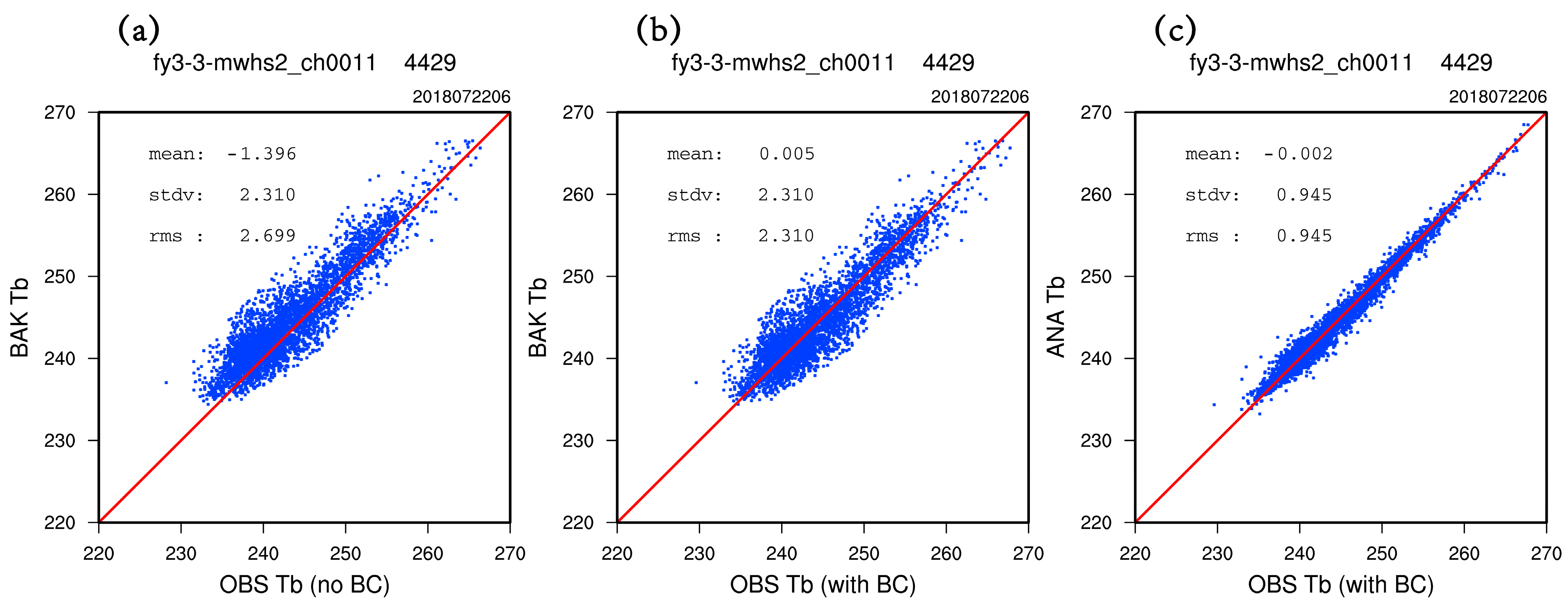
4.2. Bias Correction

Figure 5 shows the scatters of the simulated and the observed brightness temperature before and after the bias correction at 0600 UTC on 22 July 2018. The brightness temperature simulation is conducted by the RTTOV atmospheric radiative transfer model. It can be found from Figure 5a that for most scatters, the simulated values of the background field are higher than those of the observation before the bias correction. After the bias correction, it can be found from Figure 5b that the mean value of OMB is nearly equal to 0 K, indicating that the systematic bias is largely corrected. Further, after the assimilation of MWHS2, the root mean square error (RMSE) of the analyzed field is reduced from 2.310 K to 0.945 K compared with Figure 5b. The result indicates that the data assimilation method is able to adjust the moisture and temperature information appropriately to fit the observation with both the background and the observation errors considered.

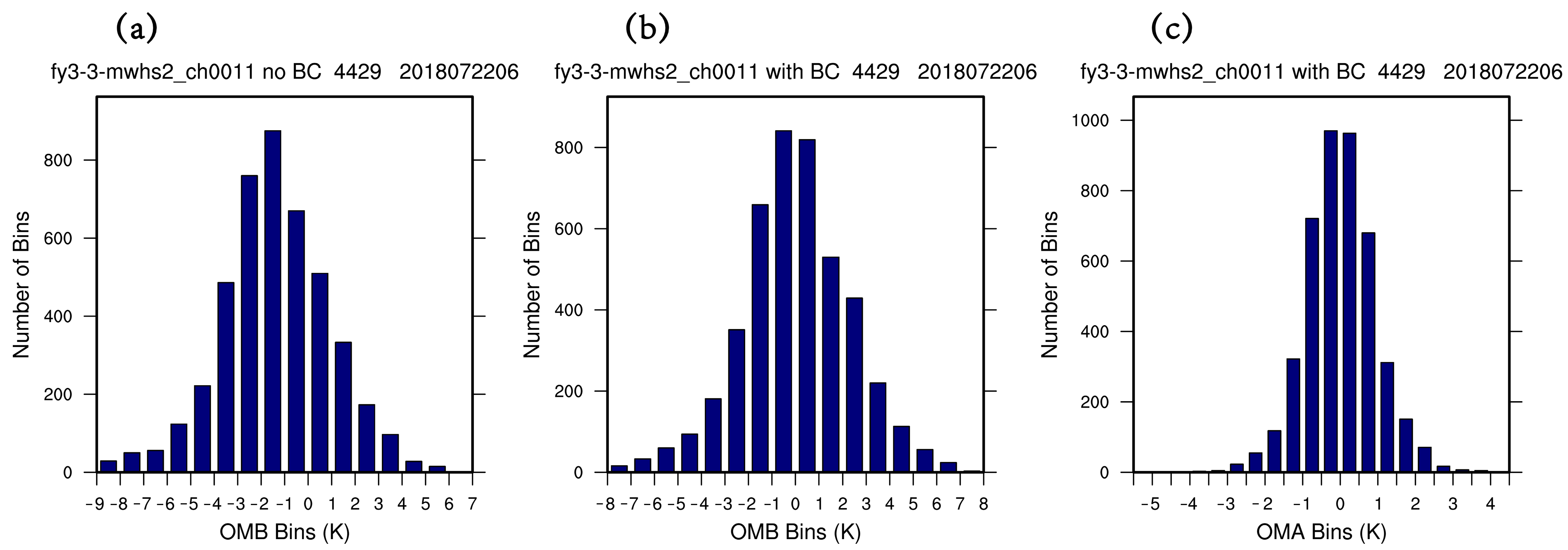
4.3. Frequency Distribution Histogram

Figure 6 shows the frequency distribution of OMB for channel 11 at 0600 UTC on 22 July 2018. Before the bias correction, it shows that most scanning points are less than 0 K with the peak between −2 K and −1 K, demonstrating that the value of most points in the background are higher than most observed ones. After the bias correction, the general distribution of OMB approximately conforms to normal distribution, with the peak moving to 0 K. By comparing the histogram of OMB with and without the bias correction, it is confirmed that the bias predictors selected are suitable and the coefficients are statistically calculated. Compared with OMB, the value of OMA is convergent to 0 K with less abnormal values, while the number of those scanning points whose values are near 0 K increases after the analysis.

4.4. Statistics for All the Channels

Figure 7 shows the statistical feature of all the assimilated channels used in the experiment. Similar to Figure 5 and Figure 6, the results of the bias correction scheme and the analysis for all the channels selected are illustrated in Figure 7. Figure 7a provides the numbers of scanning points of used channels. After the QC, the numbers of scanning points of all these channels are more than 4000, which can provide sufficient observation for assimilation. Figure 7b is the mean of OMB and OMA. Without the bias correction, the means of OMB of all channels deviate from 0 K, except channel 13. With the bias correction, the deviations are reduced and the absolute values of averaged OMB of all channels are less than 0.5 K. In contrast, the means of OMA of all channels are closer to 0 K after the bias correction. Figure 7c is the averaged standard deviations of OMB and OMA. The standard deviations of OMA are obviously smaller than OMB, especially for channels 11 to 15. The smaller means and standard deviations suggest that the analysis field is more accurate than the background field.

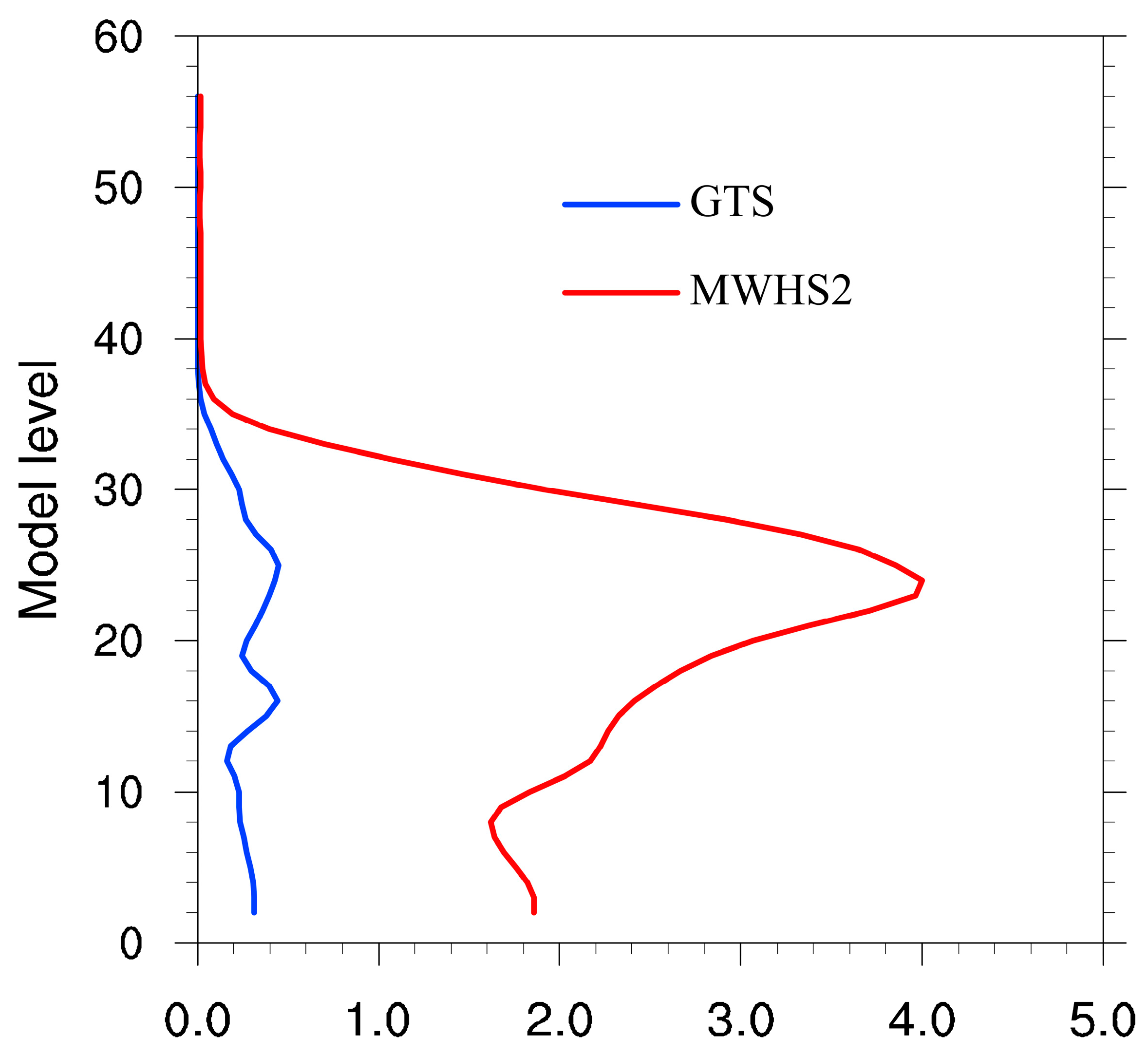
4.5. Humidity Increment RMSE

Figure 8 is the vertical increment RMSE profile of specific humidity enlarged by 10 times. The value of RMSE reflects whether these model layers are sensitive to the assimilation. It can be found that with the assimilation of the GTS data, two evident peaks appear, indicating that the assimilation of GTS data can make a difference to the lower and middle layers of the background field. In comparison, with the assimilation of the MWHS2/FY3D data, the increment RMSE of specific humidity is striking, especially below the 30th layer. The lack of water vapor information of the typhoon can be compensated for more than 0.2 g/kg for most medium and bottom levels. The large impact of humidity increment can be attributed to the abundant moisture information from the MWHS2 channels with the application of the observation operator RTTOV.

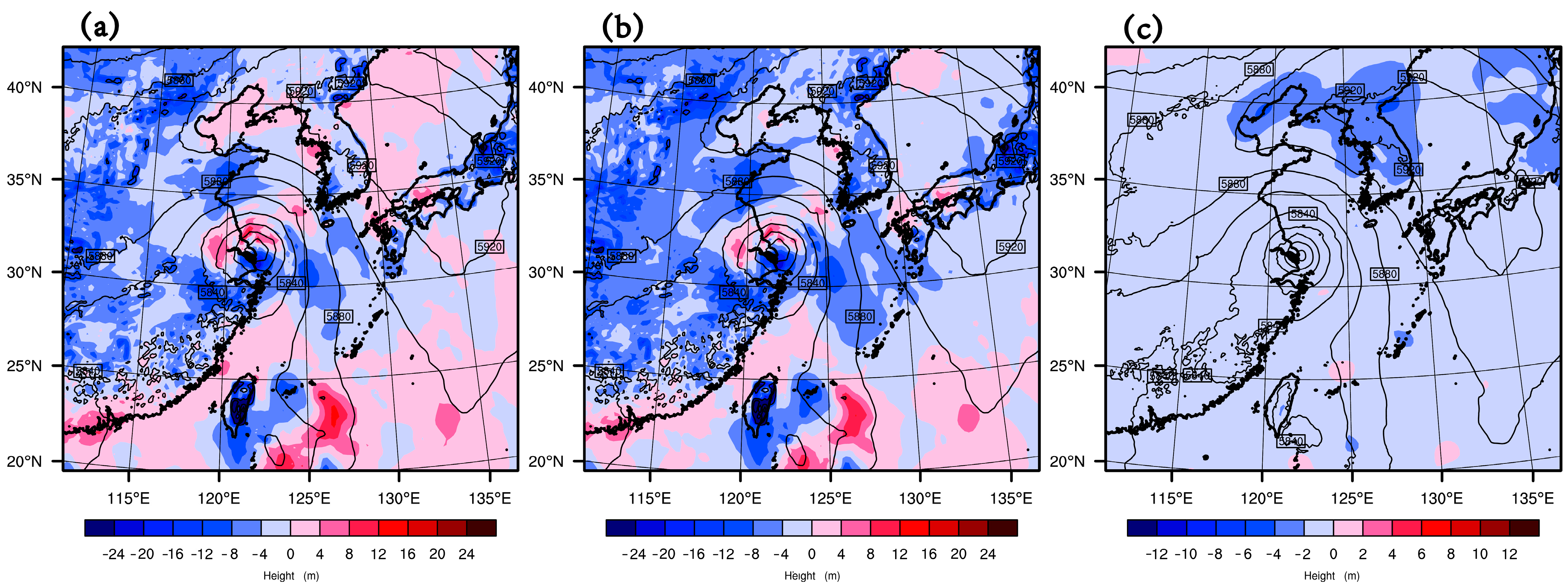
4.6. Geopotential Height Increment

Figure 9 displays the 500 hPa geopotential height increment of GTS and MWHS2. In all experiments, a negative increment near the center of the typhoon can strengthen the intensity of the typhoon. However, in their differential field, the sphere and magnitude of geopotential height increment in MWHS2 assimilation experiment are larger than those in the GTS assimilation experiment and the area of positive geopotential height increment in the north part of the typhoon is reduced, which is favorable for the intensity maintenance and the track forecast.

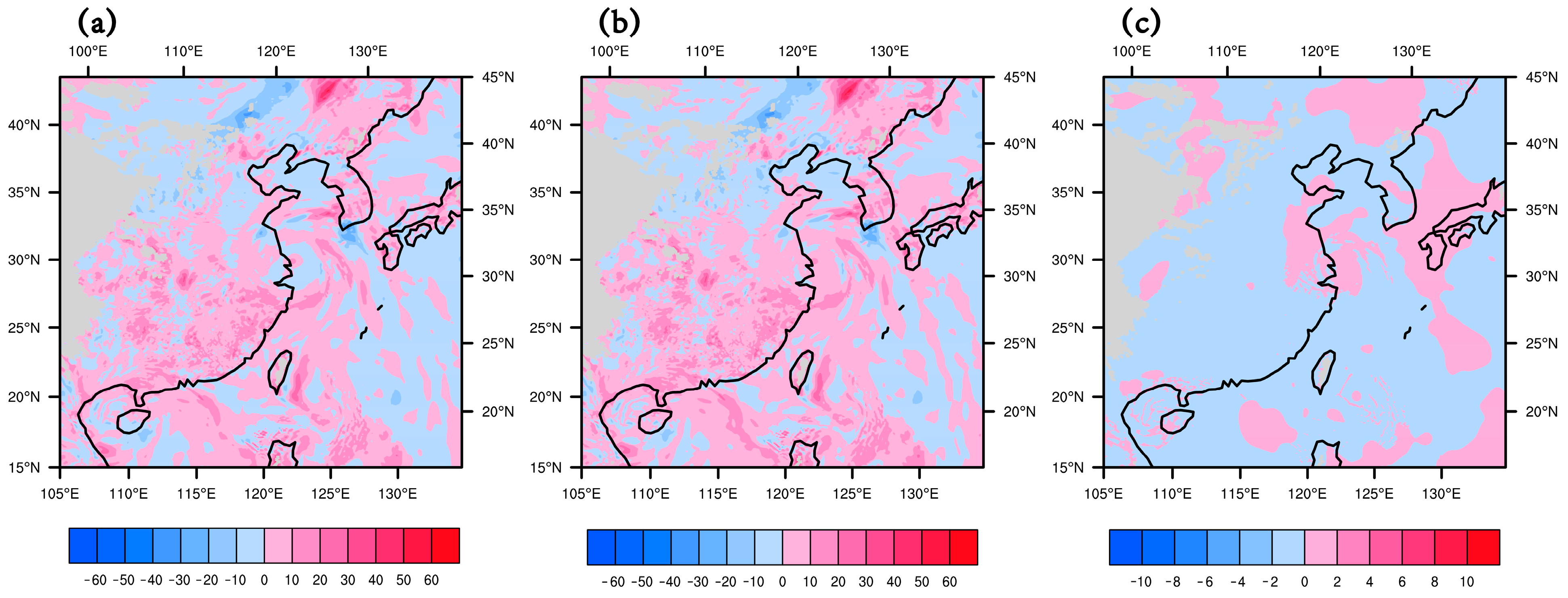
4.7. Relative Humidity Increment

Figure 10 is the increment of 850 hPa relative humidity of GTS and MWHS2. It can be found that after the assimilation of GTS data, there is a large area of positive relative humidity increment near the outer typhoon core (31.8° N, 121.7° E), and the magnitude of some regions in the spiral rain band is more than 10%. However, the value in the typhoon core is negative, which is unfavorable for the maintenance of the typhoon. By contrast, a positive relative humidity increment exists in the storm core after the assimilation of MWHS2 data, which matches well with the specific humidity increment profile shown in Figure 8. A clearer relative humidity increment near the core can be found in the differential field.

4.8. 24-Hour Accumulated Precipitation

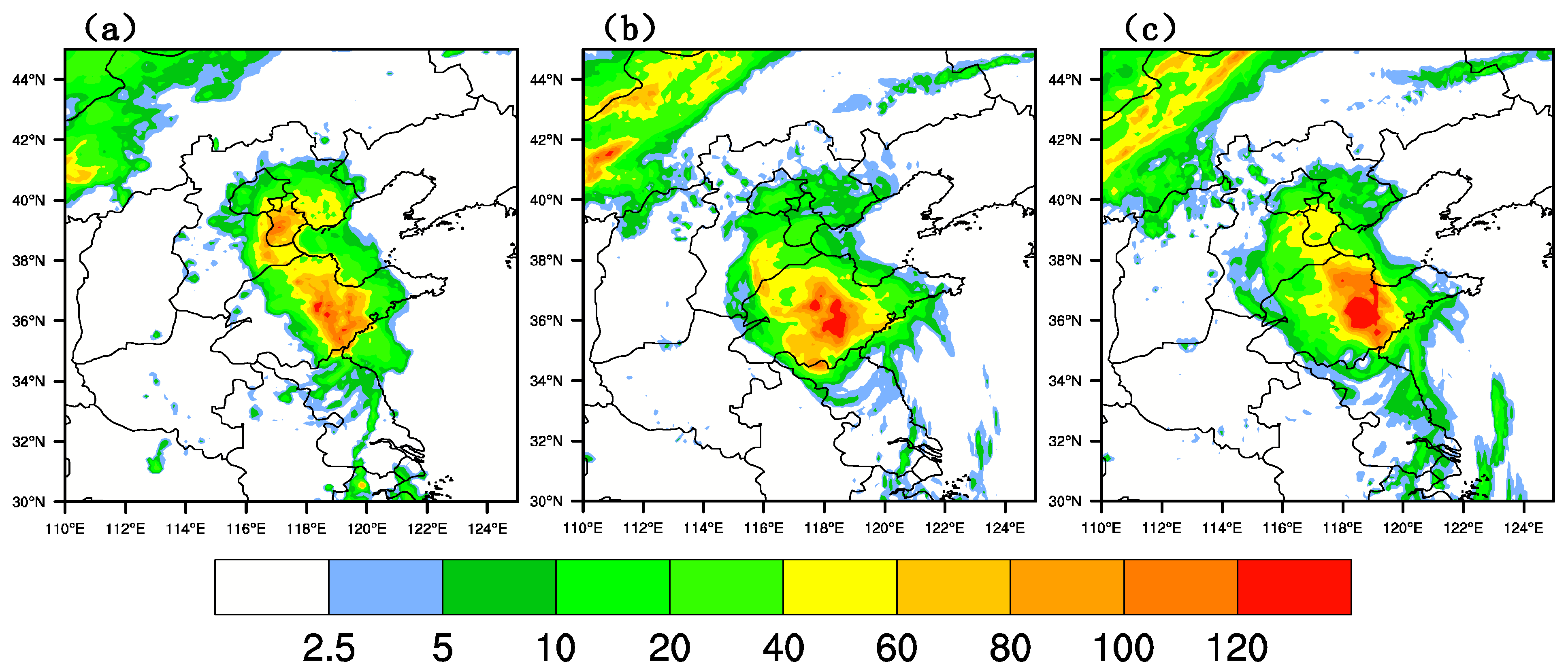
4.8.1. Rain Belt Distribution

Figure 11 provides the 24-h precipitation distribution from 0000 UTC, 23 July to 0000 UTC, 24 July. In the observation, the tropical storm Ampil brought heavy rainfall to North China, with two rainfall centers in Tianjin and Shandong. In the experiment with GTS assimilation, the rainfall center in Tianjin is underestimated, while the rainfall center in Shandong is overestimated. Besides, the two centers mismatch with the observation with a west bias. In the experiment with MWHS2 assimilation, the location of the two rainfall centers corresponds well with the observation. The forecast of the center in Tianjin is improved to some degree, and the center in Shandong is slightly overestimated.

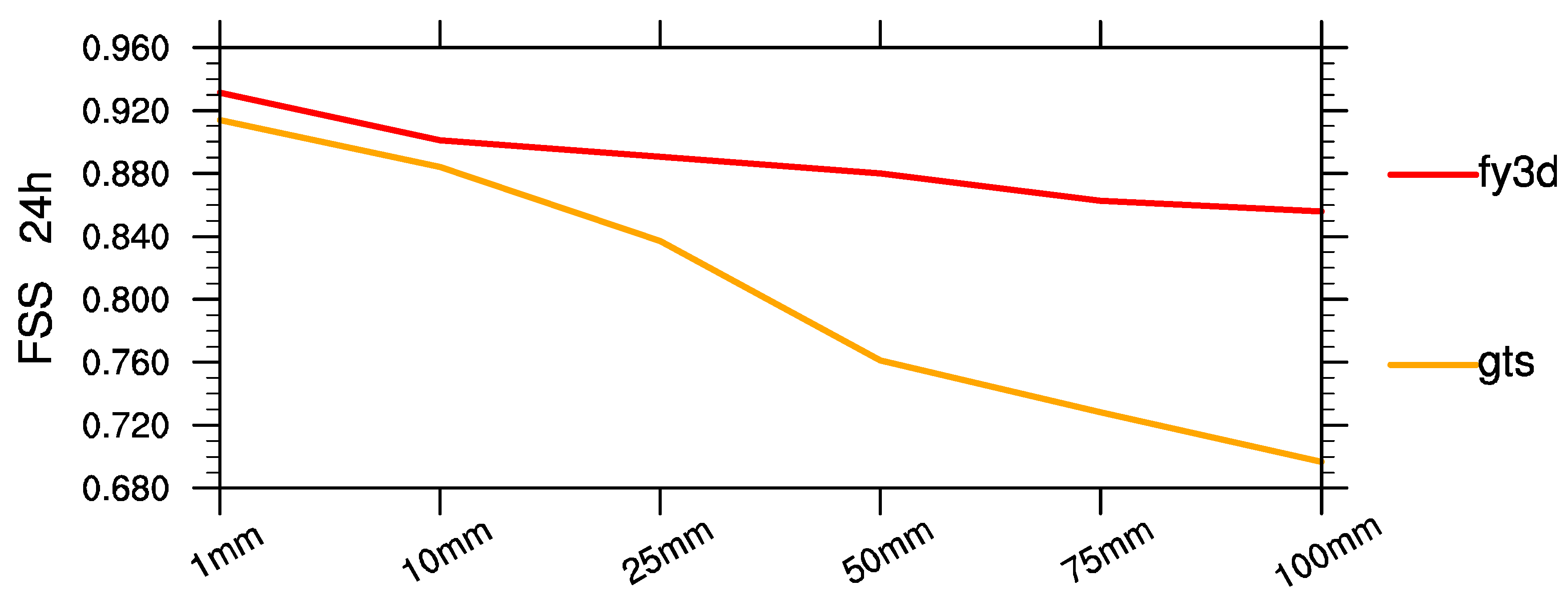
4.8.2. Fraction Skill Score (FSS) Evaluation

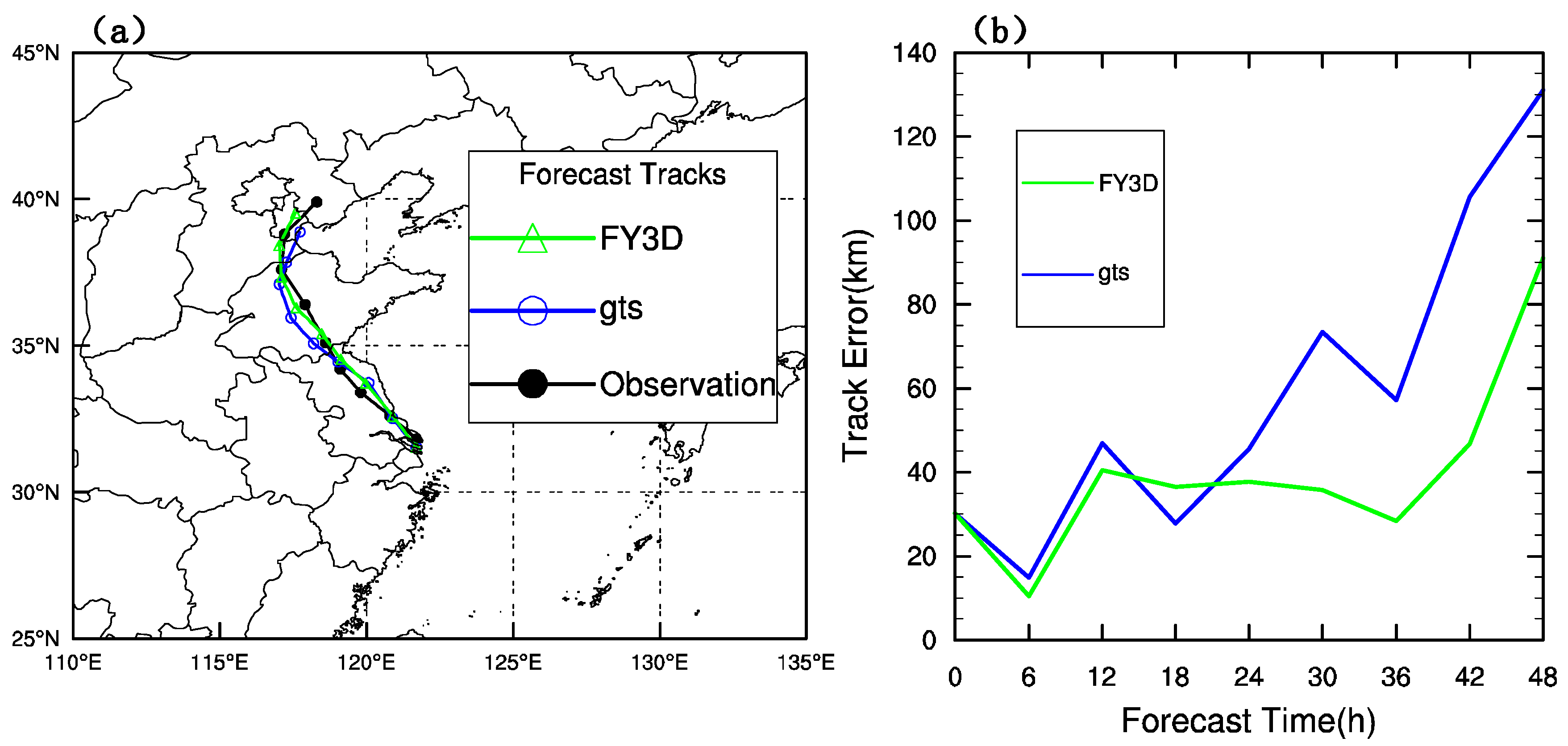
To make an objective estimate on the forecast skill of the two experiments, the fraction skill score (FSS) is employed. The FSS is defined as [44]:

$$\mathrm{FSS} = 1 - \frac{\frac{1}{N}{\displaystyle \sum _{i=1}^N}{(P_{fi} - P_{oi})}^2}{\frac{1}{N}[{\displaystyle \sum _{i=1}^N}{P}_{fi}^2 + {\displaystyle \sum _{i=1}^N}{P}_{oi}^2]}$$

where $P_{fi}$ and $P_{oi}$ represent the probabilities of forecasted and observed rainfall region, respectively, that exceeds a specific threshold value at the i-th grid point, and N represents the number of grid points in the verification region. The value of FSS is between 0 and 1, which represent no overlap and complete overlap between the forecasted and observed precipitation region, respectively.

The FSS scores of 24-h accumulated precipitation of the two experiments are shown in Figure 12. The FSS scores of the MWHS2 assimilation experiment at each threshold are higher than those of the GTS assimilation experiment. For small threshold values, the advantage of the MWHS2 experiment is not obvious, since the difference between the two experiments is small, especially below 25 mm. For thresholds larger than 50 mm, the advantage of the MWHS2 experiment is consistent and obvious.

4.9. Track Forecast

Figure 13 is the result of the 48-h deterministic forecast of the two experiments. It should be mentioned that the best track is traced by the China Meteorological Administration (CMA) [45]. Since the deterministic forecast is driven by a 6-h warm-start run, a 30 km error exists at the initial time. It can be found from the figure that in the first 12 h, the difference between the two experiments is not striking. After the integration of the model, the forecast track with the assimilation of MWHS2 is closer to the best track gradually. The track error of the MWHS2 experiment is below 40 km in the first 36 h but has a sharp increase in the last 12 h. In addition, the track error of the MWHS2 experiment is smaller than that of the GTS experiment most of the time, with a maximal error of about 90 km.

5. Conclusions and Discussion

In this study, the interface of the FY-3D MWHS2 is built in the WRFDA system. The effects of assimilating FY-3D MWHS2 radiance data under clear-sky conditions on the simulation of the tropical storm Ampil are discussed. Two numerical experiments are designed including the assimilation of the sole GTS data and the assimilation of both the GTS data and the MWHS2/FY3D radiance data. The following is concluded by these experiments:

(1)

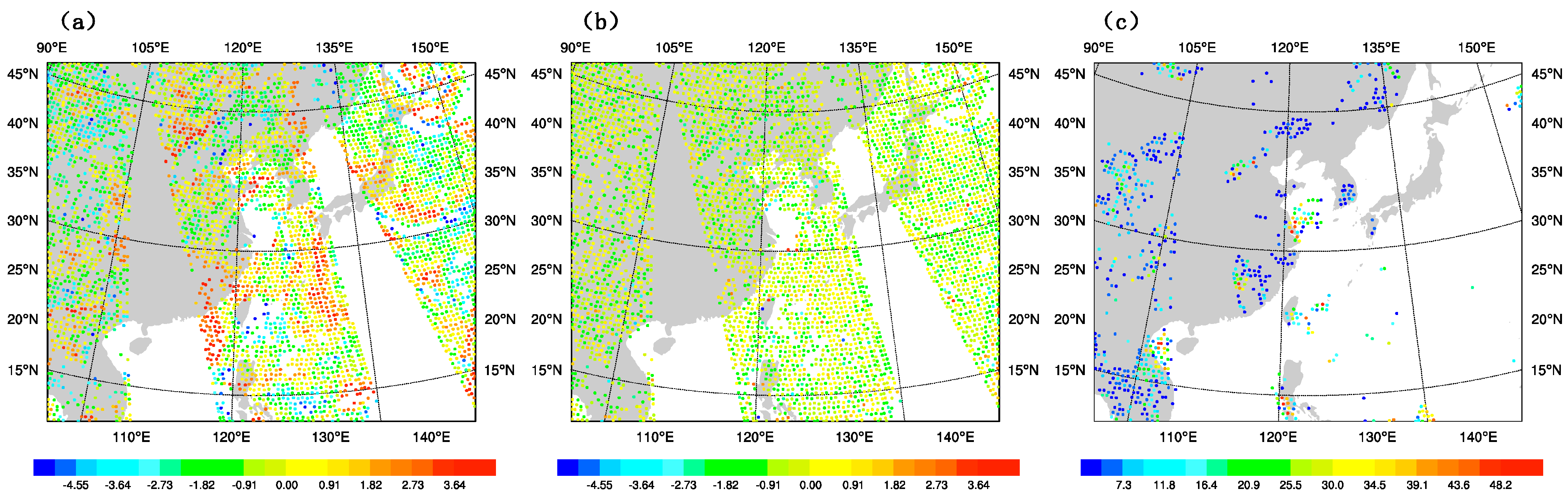
After assimilating FY-3D MWHS2 radiance data under clear-sky conditions, the notable error in the background field is strikingly reduced, and the simulated radiance of FY-3D MWHS2 matches better with the observation. By comparing the scatter diagram, the frequency distribution histogram, and the statistical line chart, it is found that the assimilation of FY-3D MWHS2 radiance data is effective.

(2)

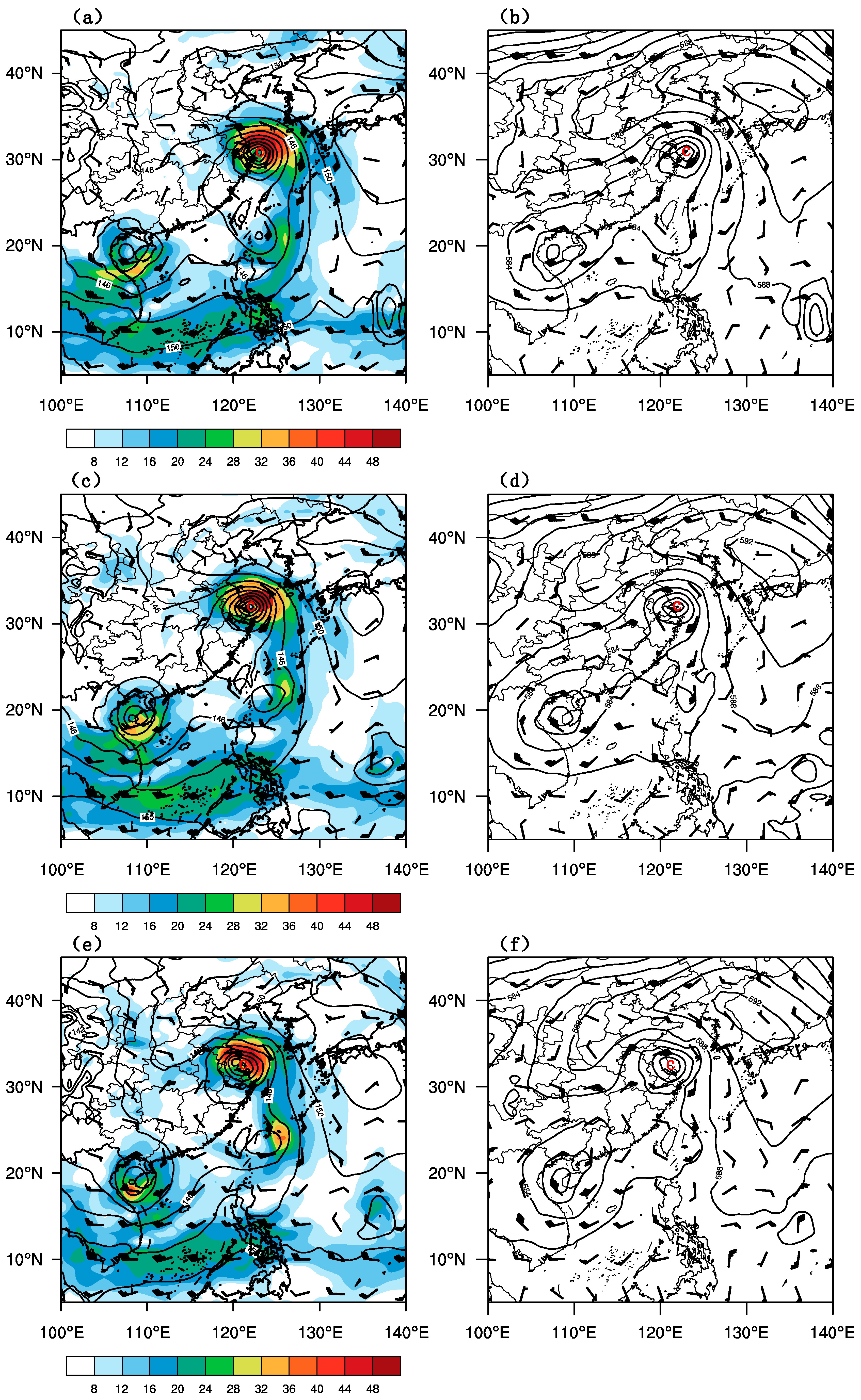
Compared with the assimilation of the GTS data, it is found that the increment of specific humidity below the 30th layer is obvious with the assimilation of the FY-3D MWHS2 radiance data. Besides, the 500 hPa geopotential height increment and the 850 hPa relative humidity increment are preferable for the maintenance of the typhoon.

(3)

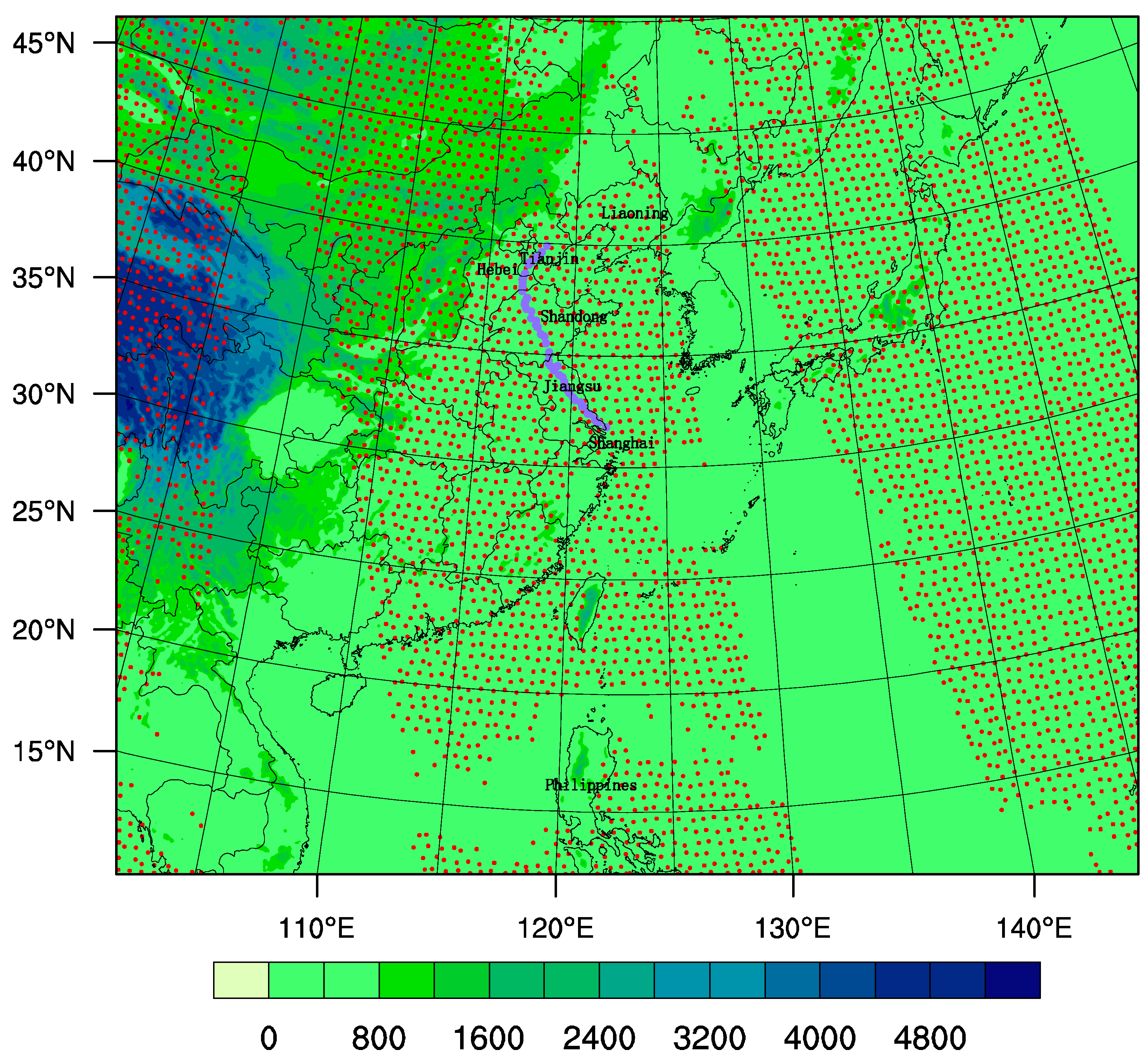
In the simulated 24-h precipitation, the position of rainfall center in the experiment with FY-3D MWHS2 assimilation shows better correspondence with the observation, whereas the rain belt in Shandong is overestimated, and the one in Tianjin is underestimated. By the quantitative FSS, the score of the FY-3D MWHS2 experiment is above 0.85 in all thresholds. In the final 48-h forecast, compared with the GTS experiment, the track error of the FY-3D MWHS2 experiment is smaller with a maximal error of roughly 90 km.

In this study, a positive influence of typhoon initialization and simulation is found for the case study of the tropical storm Ampil. It should be pointed out that this study is a preliminary attempt, since the MWHS2/FY-3D radiance data are assimilated under clear-sky conditions by the 3DVAR method with a single case. In the following work, more typhoons should be chosen to verify the effectiveness of MWHS2/FY-3D assimilation. Besides, more assimilation times (cycling assimilation) should be considered to make continuous improvements on the initial field. Last but not least, other advanced DA techniques such as the 4DVAR and the cycling methods can be applied to enhance the initialization and the forecast of typhoons with MWHS2/FY-3D radiance data.

References

1. Yao, J.; Meng, D.; Zhao, Q.; Cao, W.; Xu, Z. Nonconvex-Sparsity and Nonlocal-Smoothness-Based Blind Hyperspectral Unmixing. IEEE Trans. Image Process. 2019, 28, 2991–3006. [Google Scholar] [CrossRef] [PubMed]
2. Hong, D.; Gao, L.; Yao, J.; Zhang, B.; Plaza, A.; Chanussot, J. Graph Convolutional Networks for Hyperspectral Image Classification. IEEE Trans. Geosci. Remote Sens. 2021, 59, 5966–5978. [Google Scholar] [CrossRef]
3. Shen, F.; Xu, D.; Min, J. Effect of momentum control variables on assimilating radar observations for the analysis and forecast for Typhoon Chanthu (2010). Atmos. Res. 2019, 230, 104622. [Google Scholar] [CrossRef]
4. Sawada, M.; Ma, Z.Z.; Mehra, A. Impacts of assimilating high-resolution atmospheric motion vectors derived from Himawari-8 on tropical cyclone forecast in HWRF. Mon. Weather Rev. 2019, 147, 3721–3740. [Google Scholar] [CrossRef]
5. Xu, D.; Liu, Z.; Huang, X.; Min, J.; Wang, H. Impact of Assimilating IASI Radiance Observations on Forecasts of Two Tropical Cyclones. Meteorol. Atmos. Phys. 2013, 122, 1–18. [Google Scholar] [CrossRef] [Green Version]
6. Xu, D.; Shen, F.; Min, J. Effect of background error tuning on assimilating radar radial velocity observations for the forecast of hurricane tracks and intensities. Meteorol. Appl. 2020, 27, e1820. [Google Scholar] [CrossRef] [Green Version]
7. Ridal, M.; Dahlbom, M. Assimilation of multinational radar reflectivity data in a mesoscale model: A proof of concept. J. Appl. Meteorol. Climatol. 2017, 56, 1739–1750. [Google Scholar] [CrossRef]
8. Yang, C.; Liu, Z.; Gao, F.; Child, P.; Min, J. Impact of Assimilating GOES-Imager Clear-sky Radiance with a Rapid Refresh Assimilation System for Convection-Permitting forecast over Mexico. J. Geophys. Res. Atmos. 2017, 122, 5472–5490. [Google Scholar] [CrossRef] [Green Version]
9. Jones, T.A.; Stensrud, D.; Wicker, L. Simultaneous radar and satellite data storm-scale assimilation using an Ensemble Kalman Filter approach for 24 May 2011. Mon. Weather Rev. 2015, 143, 165–194. [Google Scholar] [CrossRef]
10. Wang, Y.B.; Liu, Z.; Yang, S.; Min, J.; Chen, L.; Chen, Y.; Zhang, T. Added value of assimilating Himawari-8 AHI water vapor radiances on analyses and forecasts for “7.19” severe storm over north China. J. Geophys. Res. Atmos. 2018, 123, 3374–3394. [Google Scholar] [CrossRef]
11. Lai, A.; Min, J.; Gao, J.; Ma, H.; Cui, C.; Xiao, Y.; Wang, Z. Assimilation of Radar Data, Pseudo Water Vapor, and Potential Temperature in a 3DVAR Framework for Improving Precipitation Forecast of Severe Weather Events. Atmosphere 2020, 11, 182. [Google Scholar] [CrossRef] [Green Version]
12. Moradi, I.; Evans, K.F.; Mccarty, W. Assimilation of satellite microwave observations over the rainbands of tropical cyclones. Mon. Weather Rev. 2020, 148, 4729–4745. [Google Scholar] [CrossRef]
13. Yang, C.; Liu, Z.; Bresch, J.; Rizvi, S.R.H.; Huang, X.; Min, J. AMSR2 all-sky radiance assimilation and its impact on the analysis and forecast of Hurricane Sandy with a limited-area data assimilation system. Tellus A 2016, 68, 30917. [Google Scholar] [CrossRef] [Green Version]
14. Bauer, P.; Moreau, E.; Chevallier, F.; O’keeffe, U. Multiple-scattering microwave radiative transfer for data assimilation applications. Q. J. R. Meteorol. Soc. 2006, 132, 1259–1281. [Google Scholar] [CrossRef] [Green Version]
15. Kim, Y.; Campbell, W.F.; Swadley, S.D. Reduction of Middle-Atmospheric Forecast Bias through Improvement in Satellite Radiance Quality Control. Weather Forecast. 2010, 25, 681–700. [Google Scholar] [CrossRef]
16. Xu, D.; Auligné, T.; Descombes, G.; Snyder, C. A method for retrieving clouds with satellite infrared radiances using the particle filter. Geosci. Model Dev. 2016, 9, 3919–3932. [Google Scholar] [CrossRef] [Green Version]
17. Zhu, Y.; Liu, E.; Mahajan, R. All-Sky Microwave Radiance Assimilation in the NCEP’s GSI Analysis System. Mon. Weather Rev. 2016, 144, 4709–4735. [Google Scholar] [CrossRef]
18. Pielke, R.A.; Landsea, C.W. Normalized hurricane damages in the United States: 1925-95. Weather Forecast. 1998, 13, 621–631. [Google Scholar] [CrossRef]
19. Franklin, J.L. National Hurricane Center Forecast Verification Report. Available online: http://www.nhc.noaa.gov/verification/pdfs/Verification_2004.pdf (accessed on 1 February 2005).
20. Shen, F.; Xue, M.; Min, J. A comparison of limited-area 3DVAR and ETKF-En3DVAR data assimilation using radar observations at convective scale for the prediction of Typhoon Saomai (2006). Meteorol. Appl. 2017, 24, 628–641. [Google Scholar] [CrossRef] [Green Version]
21. Pu, Z.X.; Yu, C.; Tallapragada, V. The impact of assimilation of GPM microwave imager clear-sky radiance on numerical simulations of Hurricanes Joaquin (2015) and Matthew (2016) with the HWRF model. Mon. Weather Rev. 2019, 147, 175–198. [Google Scholar] [CrossRef]
22. Li, J.; Liu, H. Improved hurricane track and intensity forecast using single field-of-view advanced IR sounding measurements. Geophys. Res. Lett. 2009, 36, L11813. [Google Scholar] [CrossRef]
23. Schwartz, C.S.; Liu, Z.; Chen, Y.; Huang, X.Y. Impact of assimilating microwave radiances with a limited-area ensemble data assimilation system on forecasts of Typhoon Morakot. Weather Forecast. 2012, 27, 424–437. [Google Scholar] [CrossRef]
24. Liu, Z.; Schwartz, C.S.; Snyder, C.; Ha, S.Y. Impact of assimilating AMSU-A radiances on forecasts of 2008 Atlantic tropical cyclones initialized with a limited-area ensemble Kalman filter. Mon. Weather Rev. 2012, 140, 4017–4034. [Google Scholar] [CrossRef] [Green Version]
25. Lu, Q.F. Initial evaluation and assimilation of FY-3A atmospheric sounding data in the ECMWF System. Sci. China Earth Sci. 2011, 54, 1453–1457. [Google Scholar] [CrossRef]
26. Lu, Q.; Bell, W.; Bauer, P.; Bormann, N.; Peubey, C. Characterizing the FY-3A microwave temperature sounder using the ECMWF model. J. Atmos. Ocean. Technol. 2011, 28, 1373–1389. [Google Scholar] [CrossRef]
27. Chen, K.; English, S.J.; Bormann, N.; Zhu, J. Assessment of FY-3A and FY-3B MWHS observations. Weather Forecast. 2015, 30, 1280–1290. [Google Scholar] [CrossRef]
28. Lawrence, H.; Bormann, N.; Lu, Q.F.; Geer, A.J.; English, S.J. An Evaluation of FY-3C MWHS-2 at ECMWF. EUMETSAT/ECMWF Fellowship Programme Research Report No. 37. Available online: https://www.ecmwf.int/sites/default/files/elibrary/2015/10668-evaluation-fy-3c-mwhs-2-ecmwf.pdf (accessed on 1 June 2015).
29. Zhang, P.; Chen, L.; Xian, D.; Xu, Z. Recent progress of Fengyun meteorology satellites. Chin. J. Space Sci. 2018, 38, 788–796. [Google Scholar]
30. Li, J.; Liu, G. Direct assimilation of Chinese FY-3C Microwave Temperature Sounder-2 radiances in the global GRAPES system. Atmos. Meas. Tech. 2016, 9, 3095–3113. [Google Scholar] [CrossRef] [Green Version]
31. Xian, Z.; Chen, K.; Zhu, J. All-sky assimilation of the MWHS-2 observations and evaluation the impacts on the analyses and forecasts of binary typhoons. J. Geophys. Res. Atmos. 2019, 124, 6359–6378. [Google Scholar] [CrossRef]
32. Barker, D.; Huang, X.Y.; Liu, Z.; Auligné, T.; Zhang, X.; Rugg, S.; Ajjaji, R.; Bourgeois, A.; Bray, J.; Demirtas, M.; et al. The weather research and forecasting model’s community variational/ensemble data assimilation system: WRFDA. Bull. Am. Meteorol. Soc. 2012, 93, 831–843. [Google Scholar] [CrossRef] [Green Version]
33. Li, X.; Zeng, M.J.; Wang, Y.; Wang, W.L.; Wu, H.Y.; Mei, H.X. Evaluation of Two Momentum Control Variable Schemes and Their Impact on the Variational Assimilation of Radar Wind Data: Case Study of a Squall Line. Adv. Atmos. Sci. 2016, 33, 1143–1157. [Google Scholar] [CrossRef]
34. Xu, D.; Huang, X.; Liu, Z.; Min, J. Impact of Assimilating Radiances with the WRFDA ETKF/3DVAR Hybrid System on the Prediction of Two Typhoons in 2012. J. Meteorol. Res. 2015, 29, 28–40. [Google Scholar] [CrossRef]
35. Sun, J.Z.; Wang, H.L.; Tong, W.X.; Zhang, Y.; Lin, C.Y.; Xu, D. Comparison of the Impacts of momentum control variables on high-resolution variational data assimilation and precipitation forecasting. Mon. Weather Rev. 2016, 14, 149–169. [Google Scholar] [CrossRef]
36. Zhu, Y.; Derber, J.; Collard, A.; Dee, D.; Treadon, R. Enhanced radiance bias correction in the National Centers for Environmental Prediction’s Gridpoint Statistical Interpolation data assimilation system. Q. J. R. Meteorol. Soc. 2013, 140, 1479–1492. [Google Scholar] [CrossRef]
37. Harris, B.A.; Kelly, G. A satellite radiance-bias correction scheme for data assimilation. Q. J. R. Meteorol. Soc. 2001, 127, 1453–1468. [Google Scholar] [CrossRef]
38. Auligne’, T.; McNally, A.P.; Dee, D.P. Adaptive bias correction for satellite data in a numerical weather prediction system. Q. J. R. Meteorol. Soc. 2007, 133, 631–642. [Google Scholar] [CrossRef]
39. Thompson, G.; Field, P.R.; Rasmussen, R.M.; Hall, W.D. Explicit Forecasts of Winter Precipitation Using an Improved Bulk Microphysics Scheme. Part II: Implementation of a New Snow Parameterization. Mon. Weather Rev. 2008, 136, 5095–5115. [Google Scholar] [CrossRef]
40. Hong, S.Y.; Noh, Y.; Dudhia, J. A new vertical diffusion package with an explicit treatment of entrainment processes. Mon. Weather Rev. 2006, 134, 2318–2341. [Google Scholar] [CrossRef] [Green Version]
41. Chou, M.D.; Suarez, M.J. An Efficient Thermal Infrared Radiation Parameterization for Use in General Circulation Models. NASA Tech. Memo. 1994, 3, 104606. [Google Scholar]
42. Mlawer, E.J.; Taubman, S.J.; Brown, P.D. Radiative transfer for inhomogeneous atmospheres: RRTM, a validated correlated-k model for the longwave. J. Geophys. Res. Atmos. 1997, 102, 16663–16682. [Google Scholar] [CrossRef] [Green Version]
43. Grell, G.A.; Freitas, S.R. A scale and aerosol aware stochastic convective parameterization for weather and air quality modeling. Atmos. Chem. Phys. 2014, 13, 5233–5250. [Google Scholar] [CrossRef] [Green Version]
44. Roberts, N.M.; Lean, H.W. Scale-selective verification of rainfall accumulations from high-resolution forecasts of convective events. Mon. Weather Rev. 2008, 136, 78–97. [Google Scholar] [CrossRef]
45. Ying, M.; Zhang, W.; Yu, H.; Lu, X.; Feng, J.; Fan, Y.; Zhu, Y.; Chen, D. An overview of the China Meteorological Administration tropical cyclone database. J. Atmos. Ocean. Technol. 2014, 31, 287–301. [Google Scholar] [CrossRef] [Green Version]
Figure 1. The track of tropical storm Ampil (violet dot line) covered by the scanning orbits (red dots) in the model domain overlapped by terrain height (filled colors, unit: m).
Remotesensing 13 02873 g001
Figure 2. (a,c,e) The 850 hPa circulation including geopotential height (lines, unit: dagpm), specific humidity (shading, unit: g/kg), and wind field (vectors, unit: m/s) and (b,d,f) the 500 hPa circulation including geopotential height (lines, unit: dagpm) and wind field (vectors, unit: m/s) at (a,b) 0000 UTC, (c,d) 0600 UTC, (e,f) 1200 UTC on 22 July 2018. Red “C” represents the center of tropical storm Ampil at each corresponding time.
Remotesensing 13 02873 g002
Figure 3. Distribution of GTS observations. Satellite atmospheric motion vector (SATOB), aircraft data (Airep), radiosondes (SOUND).
Remotesensing 13 02873 g003
Figure 4. (a) The OMB (unit: K), (b) the OMA (unit: K), and (c) the SI index (value > 5 K) at 0600 UTC on 22 July 2018.
Remotesensing 13 02873 g004
Figure 5. The scatter diagrams of channel 11 observed versus simulated brightness temperature (unit: K) of background (a) before the bias correction, (b) after the bias correction, and (c) observed versus simulated brightness temperature of the analysis.
Remotesensing 13 02873 g005
Figure 6. The frequency distribution histogram of (a) OMB without bias correction, (b) OMB with bias correction, and (c) OMA with bias correction of channel 11.
Remotesensing 13 02873 g006
Figure 7. (a) The numbers, (b) the means, and (c) the standard deviations of the used channels.
Remotesensing 13 02873 g007
Figure 8. Vertical increment RMSE profile of specific humidity (unit: 0.1 g/kg).
Remotesensing 13 02873 g008
Figure 9. Geopotential height increment of (a) GTS, (b) MWHS2, and (c) the difference between GTS and MWHS2.
Remotesensing 13 02873 g009
Figure 10. Relative humidity increment of (a) GTS, (b) MWHS2, and (c) the difference between GTS and MWHS2.
Remotesensing 13 02873 g010
Figure 11. Twenty-four-hour precipitation distribution of (a) observation, (b) GTS, and (c) MWHS2.
Remotesensing 13 02873 g011
Figure 12. FSS score of GTS and MWHS2.
Remotesensing 13 02873 g012
Figure 13. The deterministic forecast of (a) tracks and (b) track errors (unit: km).
Remotesensing 13 02873 g013