
Mapping Sugarcane in Central India with Smartphone Crowdsourcing
by
 , ,
, ,
Ju Young Lee
1,2,*, 
Sherrie Wang
2,3,4,
Anjuli Jain Figueroa
1,
Rob Strey
5,
David B. Lobell
1,2,
Rosamond L. Naylor
1,2 and
Steven M. Gorelick
1 1
Department of Earth System Science, Stanford University, Stanford, CA 94305, USA
2
Center on Food Security and the Environment, Stanford University, Stanford, CA 94305, USA
3
Institute for Computational and Mathematical Engineering, Stanford University, Stanford, CA 94305, USA
4
Goldman School of Public Policy, University of California, Berkeley, CA 94720, USA
5
Progressive Environmental & Agricultural Technologies, 10435 Berlin, Germany
*
Author to whom correspondence should be addressed.
Remote Sens. 2022, 14(3), 703; https://0-doi-org.brum.beds.ac.uk/10.3390/rs14030703
Submission received: 31 December 2021
/
Revised: 26 January 2022
/
Accepted: 29 January 2022
/
Published: 2 February 2022
(This article belongs to the Special Issue Big Remotely Sensed Data)
Abstract
:In India, the second-largest sugarcane producing country in the world, accurate mapping of sugarcane land is a key to designing targeted agricultural policies. Such a map is not available, however, as it is challenging to reliably identify sugarcane areas using remote sensing due to sugarcane’s phenological characteristics, coupled with a range of cultivation periods for different varieties. To produce a modern sugarcane map for the Bhima Basin in central India, we utilized crowdsourced data and applied supervised machine learning (neural network) and unsupervised classification methods individually and in combination. We highlight four points. First, smartphone crowdsourced data can be used as an alternative ground truth for sugarcane mapping but requires careful correction of potential errors. Second, although the supervised machine learning method performs best for sugarcane mapping, the combined use of both classification methods improves sugarcane mapping precision at the cost of worsening sugarcane recall and missing some actual sugarcane area. Third, machine learning image classification using high-resolution satellite imagery showed significant potential for sugarcane mapping. Fourth, our best estimate of the sugarcane area in the Bhima Basin is twice that shown in government statistics. This study provides useful insights into sugarcane mapping that can improve the approaches taken in other regions.
1. Introduction
India is the second-largest producer of sugarcane in the world, and it produced 405 million metric tons (19.7% of the world sugarcane crop) over an estimated area of 51 million ha in 2019 [1]. Sugarcane plays an important role in the country’s economy and water–food–energy security [2]. In Maharashtra, which produced 21.5% of sugarcane in India in 2019–2020 [3], water-intensive sugarcane irrigation has depleted freshwater resources and restricted irrigation of more nutritious crops [2]. An accurate recent sugarcane map is a key to assessing the impact of sugarcane cultivation on irrigation and designing targeted agricultural policies, but such a map is not available. Although there are a few existing sugarcane maps for India from global remote sensing-based projects, we found that these maps are outdated and inaccurate (see Section 2.1). The Government statistics on sugarcane area exist up to recent years, but the data are spatially aggregated and there are concerns about their accuracy [4,5,6,7]. In this study, we aimed to produce a 2019–2020 sugarcane map and estimate the sugarcane area in the Bhima Basin, which is a major sugarcane producing region in Maharashtra.
Although satellite data present an opportunity for sugarcane mapping, major issues general to any crop mapping and specific to sugarcane mapping in India still remain [8,9,10]. For example, ground-truth data are still required to train, or at least validate, models that can relate remote sensing data to crop types. However, such ground-truth data are often unavailable in many developing countries including India. Moreover, the COVID-19 pandemic condition has made it challenging to conduct any traditional field-level surveys on ground-truth data that are missing, particularly in hard-hit Maharashtra. Besides, model development has largely focused on either supervised or unsupervised methods without considering the combined use of both methods, and has not been applied much to sugarcane. In India, crop mapping efforts have mostly focused on rice, an important staple food crop which occupies the largest share of cultivated land in the country and plays a key role in the country’s groundwater depletion problem [11,12], with sugarcane receiving less attention. Some phenological characteristics of sugarcane also make mapping it quite challenging, such as a long and variable growing period of 12–18 months, different sowing and harvesting periods for different sugarcane varieties, and an extended harvest period lasting several months [10,13,14].
To fill the gap in ground-truth data, researchers are exploring the use of alternative ground-truth data including data from unmanned aerial vehicles and crowdsourcing [15,16,17,18,19]. Given the high use and increasing mobile connectivity in developing countries, mobile-phone-based crowdsourced data presents an alternative to dedicated field-level surveys. Crowdsourced data may, however, have high levels of noise and sampling bias not present in well-designed surveys but inherent in crowdsourcing. To render crowdsourced data usable as a ground-truth dataset, it is important to examine such issues and correct them. There are well-documented ways to filter to the most accurate subset of crowdsourced data, and prior work such as that in [17] has shown that the amount of data points in a subset dataset is sufficient to be used for scientific research.
For crop classification model development, there have been only limited efforts to explore hybrid methods that combine supervised and unsupervised methods. Existing studies favor supervised machine learning methods since they have outperformed unsupervised methods [20,21]. However, supervised methods require training data for every year to map crops due to potential shifts in climate and observed features. Therefore, the application of supervised methods is limited to the years with available training data, which are usually just a few recent years. Unsupervised methods do not have this limitation, since they do not require training data. In addition, unsupervised methods have several other advantages including differentiating certain crops or land covers and allowing for the discovery of unknown classes since no prior information is involved [22]. Although most existing studies used either supervised or unsupervised methods usually based on training data availability, only a few studies tested hybrid approaches that combine supervised and unsupervised methods [23,24]. These studies show that hybrid approaches produce a more accurate result than when using either of the methods separately, but these studies classified land uses and not crop types. There is a need to explore the potential of a hybrid involving both methods used for crop mapping.
For mapping sugarcane in particular, earlier studies relied on supervised methods (e.g., maximum likelihood classification, decision tree, random forest, deep convolutional neural network) and to a lesser extent unsupervised methods (e.g., ISODATA, K-means) and visual interpretation, focusing on one method or type. These studies used field-collected ground-truth data and mapped sugarcane at the pixel level of satellite data or at the segmented object level using an object-oriented approach. Geographically, these studies focused on Brazil [25,26,27,28,29] and China [30,31,32], the first- and third-largest sugarcane producing countries. Recently, a few studies have mapped sugarcane in case-study regions in Uttar Pradesh [33,34], the largest sugarcane producing state located in sub-tropical northern India. However, for Maharashtra, the second-largest sugarcane producing state in tropical central India, there have been only outdated and inaccurate sugarcane maps from global crop mapping studies. Although the previous studies produced reasonable results for sugarcane mapping in their respective study regions, more work is needed to map sugarcane and compare the performance of crop classification methods for central India.
In this study, we produced a 2019–2020 sugarcane map and estimated the sugarcane area for the Bhima Basin in Maharashtra. We utilized satellite data and novel farmer-crowdsourced geolocated crop data based on a mobile-phone app called Plantix, and used both supervised machine learning (neural network) and unsupervised classification methods individually and in combination. Regarding the use of Plantix data for crop mapping, [17] has successfully used Plantix data to map rice and cotton in southeast India, and we built on this study by expanding the use of Plantix data to sugarcane mapping in central India. We acknowledge GPS inaccuracy and sampling bias in Plantix data and took well-documented measures from [17] to filter them out and select the most accurate subset of Plantix data. Using Plantix and satellite data, we produced sugarcane maps from both supervised and unsupervised methods and then combined the two maps to produce a higher-confidence map. We validated and evaluated our maps and also compared our sugarcane areas to the government statistics.
The four major contributions of this study are as follows. First, we demonstrate that crowdsourced data can be used as an alternative ground truth for sugarcane mapping. Second, we combine supervised machine learning and unsupervised learning to create a high-confidence sugarcane map. Third, we evaluate tradeoffs among supervised, unsupervised, and hybrid classification methods for sugarcane mapping, and our findings are readily transferrable to sugarcane mapping in other regions. Fourth, our final 10 m sugarcane maps and total sugarcane area estimates provide sound information that is valuable for agricultural and water allocation policy development in the basin compared to unreliable government statistics.
The remainder of this paper is arranged as follows. Section 2 introduces the study region and explains the problems with the existing sugarcane maps for the region. Section 3 and Section 4 explain the data and methods we used, respectively. We present our results in Section 5 and discuss their implications in Section 6. Section 7 concludes with main takeaways from this paper and future research directions.
2. Study Area
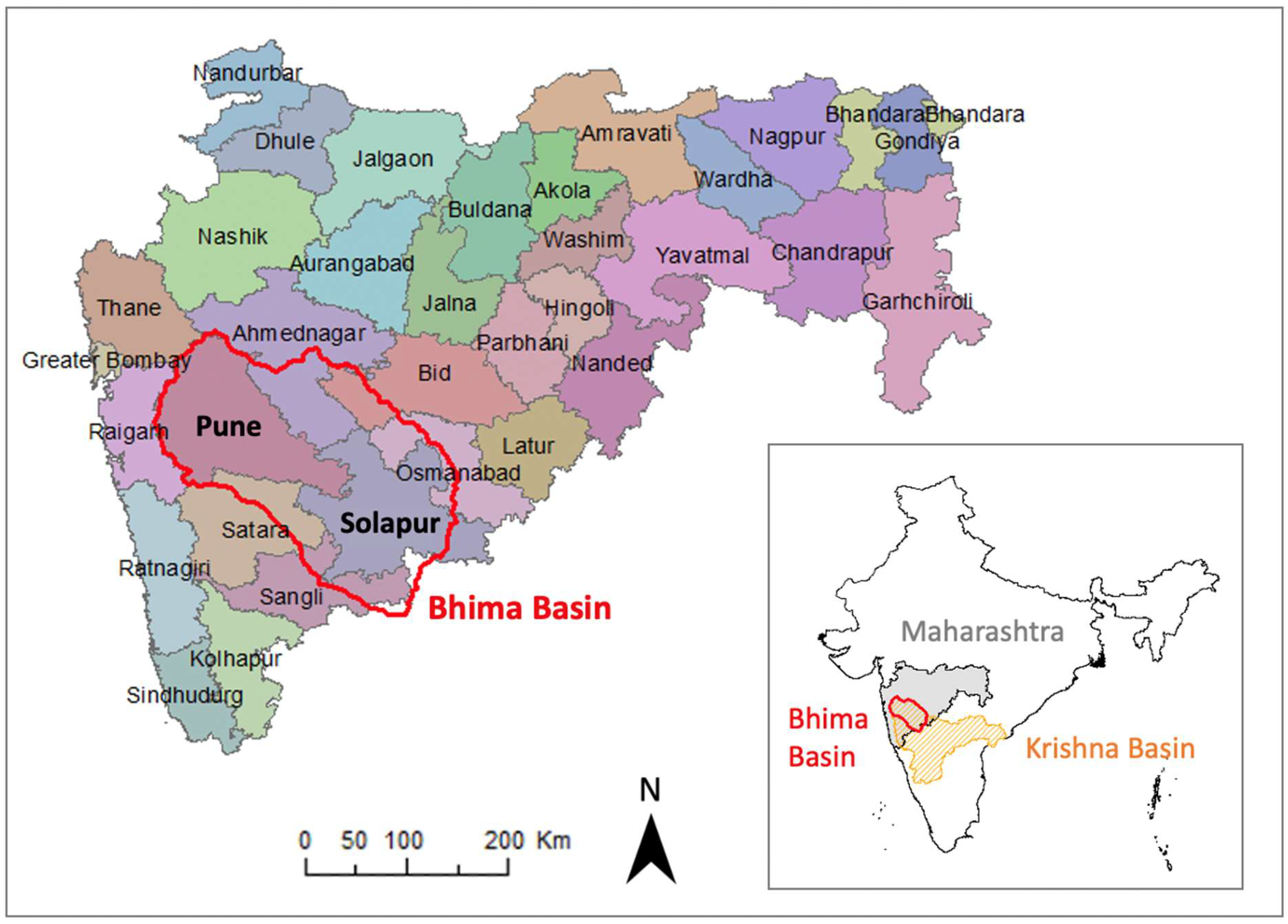
Maharashtra, located in central India, has a tropical climate with a monsoon from June to October. Located primarily in the state of Maharashtra, the Bhima Basin is delineated as the northwest portion of the Krishna Basin (Figure 1) and has an area of 45,335 km2. The uppermost part of the basin is a mountainous range, the Western Ghats. The rest of the basin, which is predominantly flat, is mostly devoted to agriculture. The Bhima Basin is a major sugarcane producing region in Maharashtra, accounting for about half of the state’s total sugarcane area [35]; according to government statistics, sugarcane area in the state has expanded from 0.1 million ha in the 1960s to 1.1 million ha in the 2010s. In this region, mapping sugarcane is challenging due to its phenological characteristics, and the existing sugarcane maps are outdated and inconsistent.
2.1. Sugarcane Phenology
Sugarcane is a perennial crop that is cultivated in tropical and subtropical regions. It forms multiple stalks that grow 2–6 m high and long sword-shaped leaves along the stalks. The crop undergoes four growth phases: germination, tillering, grand growth, and maturity. Plantation and ratooning are the two types of methods used to grow sugarcane crops. The plantation approach is to sow fresh seeds or seedlings in the field, while ratooning is allowing the stubble left in the field after harvesting to grow again without completely ploughing. A crop grown by ratooning matures early and has low yield compared to a crop grown by plantation.
In Maharashtra, three varieties of sugarcane—Adsali, preseasonal, and Suru—are cultivated. Their phenological cycles are 12–18 months, and their yields differ. For different varieties, sowing and harvesting seasons are different, and harvesting also extends over several months from October to March [36] (Figure S1). Ratooning is commonly practiced several times after harvesting the plant crop and has a growth cycle of 11 months. The three varieties and ratooning coexist over different growth cycles and yield levels vary, and these phenological characteristics of sugarcane make mapping it challenging compared to mapping other crops.
To address these challenges, we used time-series satellite data for a year as an input to our crop classifications. Our supervised and unsupervised methods did not distinguish sugarcane varieties but focused on mapping all sugarcane (see Section 4 for more details about the methods).
In Maharashtra, three varieties of sugarcane—Adsali, preseasonal, and Suru—are cultivated. Their phenological cycles are 12–18 months, and their sowing and harvesting seasons are different. Sugarcane harvesting is extended from October to March, and ratooning follows the harvest.
2.2. Existing Sugarcane Maps and Data
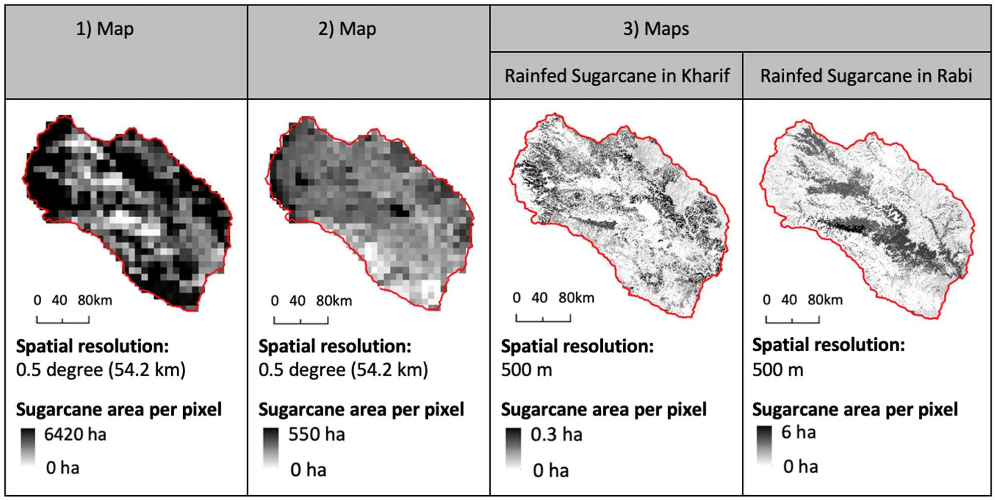
Existing sugarcane maps and data in the region are outdated and contradictory. Publicly available maps are at least 16 years old, making the spatial data outdated. Annual crop area statistics available from the Indian government are spatially aggregated at various administrative levels, so they do not provide detailed spatial distribution of sugarcane. Furthermore, these data sources have contradictions that bring into question their accuracy. For example, there are three main crop maps showing sugarcane in the basin, available from global remote sensing-based projects, but as shown in Figure 2, they are inconsistent. The two maps for the year 2000 from MIRCA2000 [37] and Monfreda’s study [38] show conflicting spatial distributions of sugarcane with different magnitudes. For the year 2005, the GEOSHARE pilot project [39] maps crops by cropping season (Kharif/Rabi/Zaid) and irrigation status (rainfed/irrigated), but the values contradict the typical growing cycle and water requirements of sugarcane in the basin. Although sugarcane is a perennial crop and grown throughout the year, GEOSHARE’s maps show sugarcane in different areas in different seasons in the basin. Moreover, sugarcane is heavily irrigated all year round in the basin, but GEOSHARE’s sugarcane maps report all of the basin’s sugarcane as rainfed due to lack of irrigation-related data for Maharashtra.
Similar to the maps in Figure 2, government data sources show inconsistencies. As seen in Table 1, 2015–2016 sugarcane areas reported by three different government sources vary substantially at both basin and district levels. For the district level comparison, we chose the Pune and Solapur districts that are almost entirely within the Bhima Basin (Figure 1). According to the assessments from international organizations such as the World Bank and FAO, as well as the Indian government, the government crop statistics in India have substantial errors due to inadequate level of resources, training, and supervision of field staff who are responsible for crop area, production, and yield estimation [4,5,6,7].
To address the data deficiencies in the existing sugarcane maps and sugarcane area data, we produced up-to-date sugarcane maps validated with field-level data crowdsourced from farmers, evaluated them with high-resolution satellite imagery, and estimated the sugarcane area (see Section 4 for more details).
3. Data
In this study, we used data from the Plantix app, satellites, and government statistics (Table 2). The free mobile app Plantix creates a novel dataset that is crowdsourced and geolocated with crop type labels. We used this for both training and validation purposes. We used various satellite data to mask non-agricultural lands, Sentinel-2 satellite data to classify sugarcane in the unmasked agricultural lands, and Google Static Map satellite images to filter Plantix data by in-field identification. We also used Google Static Map and Airbus satellite images to evaluate our sugarcane area. In addition, we compared our sugarcane area to the Indian government’s statistics on the district-level sugarcane area.
3.1. Crowdsourced Data
In the absence of conventional ground-survey data that we could use for training and validation purposes, we used a novel dataset that served as an alternative ground-truth dataset: crowdsourced data with geolocated crop type labels from a free mobile app called Plantix. Farmers submit photos of their crops to Plantix, and Plantix uses image recognition to diagnose crop pests and diseases and provides them with an advisory service. The app has been available in several states in India, including Maharashtra, since 2017. In Maharashtra, the app logged about 300,000 geolocated photos from farmers for a total 22 crop types from June 2018 to December 2020 (see Figure 3 for sugarcane and Figure S2 for rice and cotton for comparison). Based on these crop photos, the Plantix app infers crop labels as well as crop pests and diseases, using a deep convolutional neural network (DNN). The accuracy of Plantix crop type labeling varies from 78% to 100% by crop type; for sugarcane, it is 96%. Our use of Plantix data was limited to crop labels (e.g., sugarcane) rather than pest and disease diagnoses.
The Plantix dataset had two major limitations—(1) GPS inaccuracy and (2) sampling bias toward disease-prone crops. First, there is a GPS accuracy limitation in using the Plantix dataset for remote sensing-based cropland classification. Although farmers generally take photos of their crops and submit them from the reporting location, some might submit the photos from places other than their crop fields (e.g., home, cafe). Even if farmers submit their photos from their crop fields, the submitted GPS information could be somewhat inaccurate for several reasons. A second challenge of the Plantix dataset was the sampling bias inherent to the purpose of the app. Since the app is designed to diagnose crop pests and diseases, farmers submit photos of their crops that are affected by diseases, so the submissions are biased towards crops that are more prone to diseases such as vegetables (e.g., tomato, onion, and pepper).
Section 4.1 explains the measures we took to reduce the impact of these limitations, which are based on the findings of the previous work by Wang et al. [17]. Once these two limitations were addressed, the expansive crowdsourced dataset from Plantix could serve as a ground-truth dataset that was otherwise unavailable or expensive to collect in the field.
3.2. Remote Sensing Data
3.2.1. For Masking out Non-Agricultural Areas
We used various remote sensing data to mask out non-agricultural areas—for example, urban built-up areas, water bodies, forest, and natural vegetation—in our study region. For the urban mask, we used the urban built-up areas identified by the IGBP (International Geosphere-Biosphere Programme) global land cover maps at yearly intervals derived from MODIS (Moderate Resolution Imaging Spectroradiometer) Terra and Aqua reflectance data (MCD12Q1). For water bodies, we used the global water mask at 250 m spatial resolution derived from MODIS and the Shuttle Radar Topography Mission, circa 2000–2002 (MOD44W). For forest, we created a mask for the areas having elevation higher than 850 m or slope larger than 4%, using the SRTM digital elevation data from 2000 at 90 m spatial resolution. Although other studies have relied on lower elevation thresholds, such as 630 m and 750 m [42,43], we chose a threshold of 850 m based on our visual inspection of high-resolution images of the high-elevation areas. We adopted the slope criteria of 4% from the previous study done by Immerzeel et al. [42]. To mask natural trees/vegetation in the low-elevation flat region of the basin, for which the masks listed above were not effective, we checked various global land cover maps and used the one from the Copernicus Global Land Service (CGLS) at 100 m spatial resolution as it best identifies such areas. Therefore, we used additional non-cropland areas based on the CGLS land cover map.
3.2.2. For Supervised Classification
Following prior work that showed the Sentinel-2 time series successfully distinguishing certain crop types in the Indian setting [17], we used Sentinel-2 images from 1 January to 31 December 2020 as input features of the crop type classifier. Sentinel-2 is an optical Earth observation mission launched by the European Space Agency (ESA) and comprised two satellites, Sentinel-2A and Sentinel-2B. Since March 2017, the constellation has collected images on a 5-day cycle.
Sentinel-2 was chosen for its public availability and high spatial resolution of 10–60 m (depending on the bands). The 10–20 m resolution data allow crop mapping at a sub-field level in smallholder systems like those dominating the Bhima Basin. The 60 m resolution data are relatively coarse but still provide some useful signals for crop identification, as shown in [17]. The satellites’ sensors collect multi-spectral data in 13 bands; the red edge bands and short-wave infrared bands (20 m resolution) in particular have been shown previously to aid in crop type classification [17].
We accessed Sentinel-2 Level-2A imagery through the Descartes Labs platform. The Level-2A product is the result of processing using a toolbox provided by ESA to correct for atmospheric effects, and yields surface reflectance measurements. Because optical sensors cannot see through clouds, we used the Descartes Labs Sentinel-2 cloud mask to remove all pixels of clouds in our time series. We also computed the green chlorophyll vegetation index (GCVI) as an extra feature to help the model distinguish between crop types. GCVI is calculated as (NIR/Green)-1 where NIR and Green are the near-infrared and green spectral bands, respectively [44].
In total, at each latitude and longitude in our study area, we used the full cloud-free data of 13-band Sentinel-2 plus GCVI in a time series spanning 1 January to 31 December 2020 to perform crop type classification.
3.2.3. For Unsupervised Classification
For unsupervised classification, we also used the Sentinel-2 Level-2A data for the same reasons as the supervised method and for comparison with the supervised map. We used the red and near infrared bands from Sentinel-2 imagery over an agricultural year from June 2019 to May 2020 to get a time series Normalized Difference Vegetation Index (NDVI) pattern as an input for unsupervised classification. NDVI is calculated as (NIR-Red)/(NIR + Red) where NIR and RED are the near-infrared and red spectral bands, respectively [45].
We used the Sentinel-2 cloud probability product to remove pixels with more than 50% cloud probability and took the median monthly NDVI to create the time series data. We accessed and processed the Sentinel-2 imagery through the Google Earth Engine (GEE) platform, an online platform for remote sensing processing developed by Google. We conducted the entire process of unsupervised classification in GEE. The main advantages of using GEE versus multiple individual platforms are easy access to an extensive catalog of satellite imagery and other geospatial data in an analysis-ready format as well as scalable computational power from Google data centers [46].
3.2.4. Google Static Map and Airbus Images
Due to mobile phone location inaccuracy and farmers taking photos of crops for Plantix while not standing in their fields, we used very high-resolution satellite imagery from the Google Static Maps API to only accept submissions within a crop field. The Google Static Map images have a resolution of 15 cm to 1 m depending on the zoom level and latitude [47]. Based on the zoom level of 19 we used and the latitude of our study region, we estimated the resolution to be 30 cm. However, the limitation of Google Static Map images is that they do not contain the specific date when each satellite image was taken. We use Airbus red, green, blue, and near-infrared bands at 1.5 m resolution because Airbus provides multiple images throughout a year with known image dates [48]. This is high enough resolution to distinguish sugarcane. Therefore, for our additional qualitative evaluation of our 2019–2020 sugarcane maps, we used the higher-resolution Google Static Map images in combination with Airbus images. For each location, we analyzed one image from Google Static Map, most likely from 2020 since we pulled the image in 2020, and one to five Airbus images from 2020 to confirm that the field contained sugarcane. Although we used RGB images from Google Static Map, we had to use a false color scheme (RGB and near-infrared reprocessed to three bands) that approximates RGB due to Airbus use and publication terms. We accessed Airbus imagery through the Descartes Labs platform.
3.3. Government Statistics on Sugarcane Area
We also compared district-level government statistics for sugarcane area to our sugarcane area for the Pune and Solapur districts, the two districts that are almost entirely within the Bhima Basin (Figure 1). For our comparison, we needed the annual sugarcane cropped area (as opposed to harvested area) for 2019–2020. The sugarcane cropped area is larger than the harvested area since sugarcane is a perennial crop cultivated over a year. However, available 2019–2020 data from the Statistical Wing of the Agricultural Department are for the sugarcane harvested area, and sugarcane cropped data from the same department are only available for limited years (1970–1971, 1980–1981, 1990–1991, 2000–2001, and 2010–2011) at the state level for Maharashtra. Therefore, we used the average ratio of sugarcane harvested area to cropped area that we calculated from those years, 85%, to convert the 2019–2020 sugarcane harvested areas to cropped areas for Pune and Solapur districts. The calculations of these ratios and the original and converted data are presented in Table S1.
4. Method
We used both a machine learning supervised method and an unsupervised method to map sugarcane for 2019–2020. Since we focused on mapping sugarcane, our work mapped sugarcane as an individual crop and grouped all other crops. Then, we combined supervised and unsupervised maps to produce a high-confidence sugarcane map. We validated our supervised, unsupervised, and high-confidence maps with the Plantix data. In addition, we qualitatively evaluated our maps using high-resolution satellite images from Google Static Map and Airbus and compared sugarcane areas from our maps to the government statistics. The steps are shown in Figure 4 and described in detail in the following Section 4.1, Section 4.2, Section 4.3, Section 4.4 and Section 4.5.
We constructed high-quality training and test sets from Plantix data and used supervised and unsupervised classification methods to create 2019–2020 sugarcane maps. A high-confidence sugarcane map was derived as the areas identified as sugarcane in the supervised and unsupervised sugarcane maps. Our supervised, unsupervised, and high-confidence maps were validated with a test set (Plantix data selected for validation), qualitatively evaluated with high-resolution satellite imagery, and compared to the government data.
4.1. Constructing Training and Test Sets
To construct training and test sets from the Plantix data, we first filtered the Plantix data to address the two major limitations of the Plantix data: (1) GPS inaccuracy and (2) sampling bias toward disease-prone crops.
To address the GPS inaccuracy, we removed erroneous Plantix submissions. Erroneous submissions were those whose geolocations did not correspond to the crop types assigned to their mobile phone image and may have adversely affected both the supervised model’s ability to learn correct decision boundaries and our ability to assess the performance of all of our models. We removed erroneous submissions in two ways:
- We removed submissions whose GPS accuracies, as assigned by the Plantix app’s Android platform, were highly inaccurate. The exact GPS accuracy thresholds we used were different between the training and test sets; we describe them below.
- The Sentinel-2 pixel data at the submission location were classified as “in field”, “more than half in field”, “less than half in field”, and “not in field” by a separate CNN trained on in-field labels generated by human labelers and Google Static Map imagery (Figure S3). We used only the Plantix submissions that were “in field” or “more than half in field” for our training and test sets.
The sampling bias toward disease-prone crops was partly reduced when we removed Plantix submissions of vegetables, which are frequently intercropped with sugarcane, and submissions of perennial tree crops, which can be confused with sugarcane. Before excluding those crops, the share of sugarcane data in our training dataset from Plantix filtered by GPS accuracy was 1%, which is lower than the 6% actual share of sugarcane area in the total cropped area according to the government’s latest agricultural census from 2015–2016. After excluding vegetable crops from the dataset, the share of sugarcane increased to 8%, which is closer to the actual area share.
While it is important to have a clean training set to train a correct model, it is even more important to have a high-quality test set to evaluate the performance of the model [17]. Therefore, for the test dataset, we kept only submissions with GPS accuracy within 10 m, which is the Sentinel-2 spatial resolution, and submissions whose Sentinel-2 pixels were more than half inside a crop field. Because Plantix submissions were often clustered near urban areas with greater mobile phone internet access, we then sub-sampled geographically uniform points.
The training set, which excluded the test set data, was constructed by first keeping only points with GPS accuracy within 50 m and submissions that came from mostly inside a crop field. We then removed any points within 500 m of any test points to avoid inflating evaluation metrics through geographic proximity.
4.2. Supervised Classification
For supervised classification, we employed a 1D convolutional neural network (CNN) to classify sugarcane and other crops from Sentinel-2 time series data of 13 bands and GCVI. We performed the CNN training on the Descartes Labs platform, which uses resources from Google Cloud Computing. The pipeline followed the methodology in [17], which contains more detailed descriptions of each step. The time series was represented as a 14 row by 366 column matrix, where each row is a band or GCVI and each column is a day of the year (Figure A1). This encoding was chosen to standardize the Sentinel-2 time series with different observation dates to the same neural network input size. For each data point, if Sentinel-2 took a cloud-free observation on day D, the values on day D (column D of the matrix) are the band values from that day. Since the revisit time of Sentinel-2 is 5 days and there may be cloudy observations, the days with no cloud-free observations were imputed with values from the previous cloud-free observation.
We used a shallow, 4-layer CNN that convolved over the temporal dimension with kernels of size 3. Each convolutional block contained multiple convolutions followed by batch normalization, a rectified linear unit, and max pooling. The final prediction was output by a few fully connected layers.
Training was performed by minimizing the cross-entropy loss between sugarcane and other crops (Appendix A). Hyperparameters, such as the number of convolutional blocks and filters per layer, were the same as those used in [17] and not tuned on a separate test set.
Using the trained classifier, we produced a supervised crop type map. The supervised map is considered to be for January to December 2020, since most of the Plantix data were concentrated in this period. Then, we assumed that the supervised sugarcane area from January to December 2020 was also sugarcane from June 2019 to May 2020, given that sugarcane varieties cultivated in the basin have a growth duration from 12 to 18 months and sugarcane is often cultivated year after year. Therefore, we could compare these areas to the unsupervised sugarcane area we produced for June 2019 to May 2020 and the government statistics for the same period.
4.3. Unsupervised Classification
For unsupervised classification, we conducted K-means classification to classify sugarcane and other crops from Sentinel-2 time series data of NDVI. All steps of unsupervised classification were conducted in GEE, and the steps are described below.
We first calculated the monthly median NDVI over an “agricultural year” in India, which is from June 1, the beginning of Kharif (monsoon) season, through May 31 of the following year (e.g., 2019–2020 means June 2019 to May 2020). We then stacked the resulting 12 NDVI images for 2019–2020 into a single 12 image with these 12 attributes. Using the annual pattern of NDVI composed of all bands in the multi-band image, we conducted the K-means unsupervised classification to initially identify 30 classes. We chose the number of initial classes based on a rule of thumb for K-means classification, which is to use more than 5 times the final number of classes that we ultimately want to identify. Since our goal was to identify 4–6 major classes, we chose 30 as the number of initial classes for K-means unsupervised classification.
After unsupervised classification identified the 30 initial classes, we reviewed the time-series spectral signature of each class and manually categorized each class into one of the following 4 major groups—single crop, double crop, perennial crop (sugarcane), or barren land/shrub. We made such categorizations based on the number, timing, and magnitude of the peaks in the time-series NDVI throughout a year (see Figure A2 for more details). Given that it is difficult to distinguish sugarcane from other perennial crops based on NDVI alone [10,13,14] and the majority of perennial crops in the basin are sugarcane, we assumed that the perennial crops identified by our unsupervised method were sugarcane.
The features used to identify the four groups are as follows. We tested the NDVI threshold based on the approximate range of values from existing studies [10,49]; however, we saw substantial misclassification in our study region (e.g., identifying trees as sugarcane). Adopting a threshold of 0.4 reduced this misclassification.
- Single crop: Single NDVI peak (>0.4) between June and November and low NDVI (<0.4) after November.
- Double crop: Two NDVI peaks (>0.4), one between June and November and the other between December and March; the NDVI drops to less than <0.4 between the two peaks.
- Perennial crop (sugarcane): High NDVI (>0.4) throughout a year with two exceptions: 1) NDVI below 0.4 between June and October is acceptable due to noises in Sentinel-2 data during monsoon; and 2) NDVI below 0.4 up to two months between November and May is acceptable due to possible harvest in the period.
- Barren land/shrub: Low NDVI (<0.4) throughout a year.
Since our goal was to map sugarcane, we kept the sugarcane class separate and grouped the other three non-sugarcane classes that we categorized to form an unsupervised sugarcane map.
4.4. Utilizing Both Methods in Combination
We identified the areas of two 2019–2020 maps from our supervised and unsupervised classification, where these maps show sugarcane in common. We defined this as a high-confidence sugarcane map. Although we had less confidence in the remaining sugarcane area classified by either method only, we still considered it as a potential true sugarcane area and evaluated it with high-resolution satellite images from Google Static Map and Airbus.
4.5. Validation, Evaluation, and Comparison
We validated our supervised, unsupervised, and high-confidence sugarcane maps using the Plantix data that were not used for training the supervised model. We assessed precision (user’s accuracy), recall (producer’s accuracy), overall accuracy, F1 score, and Kappa coefficient, using the following equations [50]:
where Po is the proportion of observed agreement, and Pe is the proportion of agreements expected by chance. The precision metric quantifies the ability of the predictor not to label as positive a sample that is negative, whereas the recall metric quantifies the ability of the predictor to find all the positive samples. The overall accuracy, F1 score, and Kappa coefficient metrics are common effectiveness measures to evaluate a classifier’s performance.
In addition, we qualitatively evaluated our sugarcane maps, using visual inspection of high-resolution satellite images from Google Static Map and Airbus. First, we compared those images at the Plantix data points that were labeled as sugarcane and other crops to identify visually distinguishable features of sugarcane. Then, using those features, we evaluated 1000 randomly selected points each from our supervised, unsupervised, and high-confidence maps. For each point, we reviewed one image from Google Static Map, which was likely from 2020, and all Airbus images available from 2020 and that labeled the point as sugarcane or not. To avoid human labeling bias, we mixed each set of 1000 points with another 1000 points sampled from regions that all of our models predicted as non-cane. We (author J.L.) also conducted this evaluation in a blind manner without knowing the prediction from our models. Due to uncertainties inherent in visually distinguishing sugarcane features and because we did not visually sample every pixel, we do not consider this approach adequate for spatial mapping validation purposes. As such, we only used the images for statistical evaluation of our sugarcane area, rather than providing explicit mapped information about where sugarcane occurs.
Lastly, we compared our sugarcane area estimates to the 2019–2020 government statistics on sugarcane areas. As explained in Section 3.3, we converted the government reported sugarcane “harvested” area for 2019–2020 to sugarcane “cropped” area for our comparison. We made our comparison at the district level for Pune and Solapur, since the basin-level sugarcane area data for 2019–2020 are not available from government sources.
5. Results
5.1. Training and Test Sets from Plantix Data
The CNN for in-field identification was found to have 0.90 accuracy on a hold-out test set when distinguishing between whether the Sentinel-2 pixel at the center of the Static Map image was more or less than half inside a field. Out of 292,379 submissions from Maharashtra between 2018 and 2020, 11,347 submissions were selected for the training set. The test set included 1425 and 165 submissions from 2020 for Maharashtra and Bhima Basin, respectively. Figure 5 shows the raw and selected high-quality Plantix submissions that we used for training and test sets on the Maharashtra map, and Table 3 summarizes the number of submissions included in our final training and test sets.
5.2. Sugarcane Maps and Validation Results
Our three sugarcane maps and validation results are presented in Figure 6: supervised, unsupervised, and high-confidence maps. The performance of our three classification methods and their tradeoffs and respective strengths are discussed in Section 6.1.
5.3. Qualitative Evaluation of Sugarcane Maps
By comparing the Google Static Map and Airbus images from the Plantix data for sugarcane and other crops, we identified the qualitative features of sugarcane fields such as a lush green color and particular vegetation texture (Figure 7). Using these sugarcane features, we found that 72%, 61%, and 86% of the randomly selected points we evaluated appeared to be sugarcane in our supervised, unsupervised, and high-confidence maps, respectively. Figure 8b shows all 3000 points that we evaluated including those points that we evaluated as sugarcane. These points are consistent when compared to Figure 8a, which shows our models’ sugarcane prediction. Another finding from this evaluation is that 10% of the points in the unsupervised maps appeared to be trees or pastures whereas the share was 5% in the supervised and high-confidence maps. Figures S4, S5, and Table S2 include more details about the evaluation result.
5.4. Comparison to Government Statistics
We compared our conservative and best estimates for 2019–2020 sugarcane area for the Pune and Solapur districts to the government data for the same year. We found our conservative and best estimates in the high-confidence and supervised maps, respectively, and how we determined that these maps were the conservative and best estimates will be explained in Section 6. As shown in Table 4, while even the conservative high-confidence map shows about 30% more sugarcane area than the government data, our best-performing supervised map shows more than twice as large a sugarcane area.
6. Discussion
6.1. Performance of Sugarcane Mapping Methods
Our supervised map performed best among the three maps we produced, since its 0.77 overall accuracy, 0.75 F1 score, and 0.55 Kappa were the highest. The unsupervised method that relied on NDVI alone did not perform well: it confused natural trees and pastures with sugarcane, as they can have similar temporal-spectral behavior to sugarcane. However, although the unsupervised map’s sugarcane precision was low (0.62), it still captured a generally similar spatial distribution of sugarcane to the supervised map. Moreover, the unsupervised method effectively improved sugarcane precision to 0.94 when combined with the supervised map to create a high-confidence map. Although the sugarcane recall worsened to 0.36 for the high-confidence map, such tradeoff between precision and recall is inevitable [51]. The high sugarcane precision of 0.94 paired with very low sugarcane recall of 0.36 suggests that the areas classified as sugarcane in the high-confidence map are highly accurate, but the map is conservative and most likely misses some actual sugarcane area.
All three maps we produced are useful for different purposes. For example, the best-performing supervised map is most suitable for analyses such as hydrologic assessment that require a detailed spatial distribution of all sugarcane. The unsupervised method produces a roughly accurate spatial distribution of sugarcane, which is still useful for some policy development, especially in the absence of any prior knowledge or training data. The high-confidence map serves as a lower bound for true sugarcane area and helps with sampling actual sugarcane fields for research or policy purposes.
There are other sugarcane mapping studies for Uttar Pradesh in India and outside India that achieved a higher overall accuracy and Kappa than our best-performing supervised map. However, their study regions were smaller than ours, and the study regions outside India had fewer crop types [28,30,32]. Sugarcane mapping in India can generally be more challenging than other regions due to: (1) small farm size, which causes spectral mixing, and (2) a limited amount of usable optical satellite data due to cloudy images during the monsoon season. After we removed cloudy Sentinel-2 images, some pixels had no usable data for the entire monsoon season from June to October. Another potential challenge for our study was the quality of our final training and test sets. Although we took several measures to select a high-quality subset of Plantix data, it is possible that our final sets still included some erroneous or biased data. The raw Plantix crop labels were also imperfect, as explained in Section 3.1. Both factors could have negatively affected our crop classification and validation performances. Potential solutions to improve our model performance include using radar remote sensing data and further improving the quality of final training and test sets.
6.2. Potential of High-Resolution Image Classification for Sugarcane Mapping
Our evaluation results from high-resolution satellite images were consistent with our validation results, which confirms our model performance and suggests the potential of high-resolution image classification for sugarcane mapping. In this study, a human labeler reviewed the images at selected points only to evaluate our sugarcane maps, but machine learning image classification can be employed to classify sugarcane at pixel or object levels for the entire basin to produce a sugarcane map. Such a model may improve our model performance when combined with our best-performing supervised model.
6.3. Government Underestimation of Sugarcane Area
For proper policy development for sugarcane agriculture, it is important to have an accurate estimate of sugarcane area. Our best-performing supervised sugarcane map shows a sugarcane area that is twice that of the government-reported area, and even our conservative high-confidence map shows the area is 30% larger. This information could help the Indian government’s efforts to address crop area underestimation in their crop statistics. The government review of the crop statistics system (APS) in India for 2017–2018 concluded that there is a general trend to underestimate crop areas [4]. For sugarcane in Maharashtra, the report found a 30% underestimation. Another government report from the Ministry of Statistics for 2016–2017 found that the sugarcane area in Maharashtra was underestimated by about 50% [5]. These assessments might still be insufficient, however, as they were made based on senior supervisory staff’s review of the same data collected by field staff with known problems of inadequate level of resources, training, and supervision. As shown in our study, satellite data analysis coupled with crowdsourced data can be a more accurate, rapid, and economical method for sugarcane mapping and area estimation, supplementing or replacing the costly and time-consuming traditional field survey.
7. Conclusions
In India, the second-largest sugarcane-producing country, accurate sugarcane maps are needed for food, water, and energy policy development and analysis. Although crop mapping in India has focused on rice, there have been few sugarcane mapping efforts, and existing sugarcane maps from published literature disagree. The challenges for sugarcane mapping in India include the lack of ground-truth data and confounding phenological characteristics (e.g., long and variable growing period of 12–18 months, different sowing and harvesting periods for different sugarcane varieties, and an extended harvest period).
Building on previous work that used smartphone crowdsourced data with supervised machine learning classification to map rice and cotton [17], we focused on the challenging task of sugarcane mapping. We showed that these challenges can be overcome using smartphone crowdsourcing data to produce reliable sugarcane maps and consequent sugarcane area estimates in India. Our sugarcane area estimate in the Bhima Basin in central India is twice as large as the government’s estimate. In addition to producing a supervised sugarcane map, we created an unsupervised sugarcane map and took the sugarcane areas in common in the supervised and unsupervised maps to construct a high-confidence sugarcane map. By evaluating the three sugarcane maps, we examined the tradeoffs among them and their respective strengths.
Smartphone crowdsourcing has great potential to be a more widely available source of ground-truth data. We showed that this approach greatly improves sugarcane mapping when crowdsourced data are carefully curated to remove errors. Through our analysis, we demonstrated that machine learning image classification using high-resolution satellite imagery with crowdsourced field data has significant potential for sugarcane mapping. Future research effort is needed to produce time series of sugarcane maps to assess the trajectory of sugarcane expansion and its impacts on food, water, and energy resources.
Supplementary Materials
The following supporting information can be downloaded at: https://0-www-mdpi-com.brum.beds.ac.uk/article/10.3390/rs14030703/s1, Figure S1: Sugarcane crop calendar in Maharashtra; Figure S2: Map and submission times of Plantix dataset for rice and cotton; Figure S3: Sample Google Static Map images for in-field classification; Figure S4: Example Google Static Map and Airbus images of randomly selected points from our lower confidence sugarcane area points that appear to be a) sugarcane, b) other crops, c) non-agricultural lands, and d) trees/pastures; Figure S5: Sensitivity analysis with total number of points evaluated; Table S1: Average ratio of sugarcane harvested to cropped area in Maharashtra; Table S2: Evaluation results from high-resolution satellite images.
Author Contributions
Conceptualization, J.Y.L., S.W., and A.J.F.; data curation, J.Y.L. and S.W.; formal analysis, J.Y.L. and S.W.; funding acquisition, S.M.G.; investigation, J.Y.L. and S.W.; methodology, J.Y.L., S.W., A.J.F., and S.M.G.; project administration, J.Y.L.; resources, R.S.; software, J.Y.L. and S.W.; supervision, D.B.L., R.L.N., and S.M.G.; validation, J.Y.L. and S.W.; writing—original draft, J.Y.L. and S.W.; writing—review and editing, J.Y.L., S.W., A.J.F., D.B.L., R.L.N., and S.M.G. All authors have read and agreed to the published version of the manuscript.
Funding
This work was supported by US National Science Foundation (NSF) grant ICER/EAR1829999 to Stanford University under the Belmont Forum Sustainable Urbanisation Global Initiative (SUGI)/Food-Water-Energy Nexus theme. Any opinions, findings, and conclusions or recommendations expressed in this material do not necessarily reflect the views of the NSF.
Institutional Review Board Statement
Not applicable.
Informed Consent Statement
Not applicable.
Data Availability Statement
The satellite remote sensing data used in this study are publicly available. Restrictions apply to the availability of the Google Static Map images, Airbus images, and Plantix data. Google Static Map and Airbus images were obtained from Google Static Map API and Descartes Labs platform, respectively, using authors’ memberships on those platforms. Plantix data was obtained from Progressive Environmental & Agricultural Technologies (PEAT), the developer of the Plantix application, and are available from PEAT.
Acknowledgments
The Plantix dataset was provided by PEAT. The authors thank Karan Raut and Ravindra Botve at PEAT for their technical support for the Plantix data analysis and the fruitful discussions on the Indian agricultural systems and data. We also thank Descartes Labs for enabling access to large-scale, high-resolution satellite imagery and for providing cloud computing for supervised sugarcane map creation.
Conflicts of Interest
The authors declare no conflict of interest. The funders had no role in the design of the study; in the collection, analyses, or interpretation of data; in the writing of the manuscript, or in the decision to publish the results.
Appendix A
Appendix A.1. More Details on Supervised Classification Method
Our training was performed by minimizing the cross entropy loss, defined as a function of input sample as
for model parameters θ, number of classes C, the input time series x, crop type probabilities , and one-hot ground-truth label y. The notation yc denotes the cth element of the vector y, which is equal to 1 if the sample belongs to class c and 0 otherwise. The element is the predicted probability that the sample belongs to class c. Minimizing cross entropy incentivizes the network to maximize the value of for the correct class c [17].
Figure A1.
Representation of time series satellite data for 1D convolutional neural network. These show example time series data of GCVI acquired by Sentinel-2 over the course of a year and formatted to be input to the 1D CNN.
Figure A1.
Representation of time series satellite data for 1D convolutional neural network. These show example time series data of GCVI acquired by Sentinel-2 over the course of a year and formatted to be input to the 1D CNN.

Appendix A.2. Spectral Signatures of Unsupervised Classes
Figure A2.
Spectral signatures for 30 unsupervised classes (Sentinel-2 time-series NDVI): (a) single crop, (b) double crop, (c) perennial crop (sugarcane), and (d) barren lands/shrub. Based on the number, timing, and magnitude of the peaks (explained in Section 4.3), we categorized each class into one of the four crop groups.

References
- Food and Agriculture Organization’s Statistical Database (FAOSTAT). Country-Wise Sugarcane Area and Production Data from 2019. Available online: http://www.fao.org/faostat/en/#data/QC (accessed on 1 November 2021).
- Lee, J.Y.; Naylor, R.L.; Figueroa, A.J.; Gorelick, S.M. Water-Food-Energy challenges in India: Political economy of the sugar industry. Environ. Res. Lett. 2020, 15, 084020. [Google Scholar] [CrossRef]
- Commission for Agricultural Costs and Prices (CACP); Ministry of Agriculture; Government of India. Price Policy for Sugarcane: The 2020-21 Sugar Season. 2019. Available online: http://cacp.dacnet.nic.in/ViewQuestionare.aspx?Input=2&DocId=1&PageId=41&KeyId=709 (accessed on 1 November 2021).
- Ministry of Statistics & Programme Implementation (MOSPI); Government of India. Review of Crop Statistics System in India, 2017–2018. 2019. Available online: http://mospi.nic.in/sites/default/files/publication_reports/AISR_2017_18_20jan21.pdf (accessed on 1 November 2021).
- Ministry of Statistics & Programme Implementation (MOSPI); Government of India. Consolidated Results of Crop Estimation Survey on Principal Crops, 2016–2017. 2019. Available online: http://mospi.nic.in/sites/default/files/publication_reports/CES_2016_17_20jan21.pdf (accessed on 1 November 2021).
- Food and Agriculture Organization (FAO). Guidelines on Improving and Using Administrative Data in Agricultural Statistics. 2018. Available online: http://www.fao.org/3/ca6413en/ca6413en.pdf (accessed on 1 November 2021).
- World Bank and Global Facility for Disaster Reduction and Recovery. Enhancing Crop Insurance in India. 2011. Available online: https://www.gfdrr.org/sites/default/files/publication/Enhancing%20Crop%20Insurance%20in%20India%20%281%29.pdf (accessed on 1 November 2021).
- Molijn, R.A.; Iannini, L.; Vieira Rocha, J.; Hanssen, R.F. Sugarcane productivity mapping through C-band and L-band SAR and optical satellite imagery. Remote Sens. 2019, 11, 1109. [Google Scholar] [CrossRef] [Green Version]
- Bégué, A.; Arvor, D.; Bellon, B.; Betbeder, J.; De Abelleyra, D.; PD Ferraz, R.; Lebourgeois, V.; Lelong, C.; Simoes, M.; Verón, S.R. Remote sensing and cropping practices: A review. Remote Sens. 2018, 10, 99. [Google Scholar] [CrossRef] [Green Version]
- Som-ard, J.; Atzberger, C.; Izquierdo-Verdiguier, E.; Vuolo, F.; Immitzer, M. Remote sensing applications in sugarcane cultivation: A review. Remote Sens. 2021, 13, 4040. [Google Scholar] [CrossRef]
- Manjunath, K.R.; More, R.S.; Jain, N.K.; Panigrahy, S.; Parihar, J.S. Mapping of rice-cropping pattern and cultural type using remote-sensing and ancillary data: A case study for South and Southeast Asian countries. Int. J. Remote Sens. 2015, 36, 6008–6030. [Google Scholar] [CrossRef]
- Xiao, X.; Boles, S.; Frolking, S.; Li, C.; Babu, J.Y.; Salas, W.; Moore III, B. Mapping paddy rice agriculture in South and Southeast Asia using multi-temporal MODIS images. Remote Sens. Environ. 2006, 100, 95–113. [Google Scholar] [CrossRef]
- Bégué, A.; Lebourgeois, V.; Bappel, E.; Todoroff, P.; Pellegrino, A.; Baillarin, F.; Siegmund, B. Spatio-temporal variability of sugarcane fields and recommendations for yield forecast using NDVI. Int. J. Remote Sens. 2010, 31, 5391–5407. [Google Scholar] [CrossRef] [Green Version]
- Shashikant, V.; Mohamed Shariff, A.R.; Wayayok, A.; Kamal, M.R.; Lee, Y.P.; Takeuchi, W. Utilizing TVDI and NDWI to Classify Severity of Agricultural Drought in Chuping, Malaysia. Agronomy 2021, 11, 1243. [Google Scholar] [CrossRef]
- Wu, F.; Wu, B.; Zhang, M.; Zeng, H.; Tian, F. Identification of Crop Type in Crowdsourced Road View Photos with Deep Convolutional Neural Network. Sensors 2021, 21, 1165. [Google Scholar] [CrossRef]
- Hegarty-Craver, M.; Polly, J.; O’Neil, M.; Ujeneza, N.; Rineer, J.; Beach, R.H.; Lapidus, D.; Temple, D.S. Remote crop mapping at scale: Using satellite imagery and UAV-acquired data as ground-truth. Remote Sens. 2020, 12, 1984. [Google Scholar] [CrossRef]
- Wang, S.; Di Tommaso, S.; Faulkner, J.; Friedel, T.; Kennepohl, A.; Strey, R.; Lobell, D.B. Mapping crop types in southeast india with smartphone crowdsourcing and deep learning. Remote Sens. 2020, 12, 2957. [Google Scholar] [CrossRef]
- Zhou, N.; Siegel, Z.D.; Zarecor, S.; Lee, N.; Campbell, D.A.; Andorf, C.M.; Nettleton, D.; Lawrence-Dill, C.J.; Ganapathysubramanian, B.; Kelly, J.W.; et al. Crowdsourcing image analysis for plant phenomics to generate ground truth data for machine learning. PLoS Comput. Biol. 2018, 14, e1006337. [Google Scholar] [CrossRef] [Green Version]
- See, L.; McCallum, I.; Fritz, S.; Perger, C.; Kraxner, F.; Obersteiner, M.; Deka Baruah, U.; Mili, N.; Kalita, N.R. Mapping cropland in Ethiopia using crowdsourcing. Int. J. Geosci. 2013, 4, 6–13. [Google Scholar] [CrossRef] [Green Version]
- Larrañaga, A.; Álvarez-Mozos, J.; Albizua, L. Crop classification in rain-fed and irrigated agricultural areas using Landsat TM and ALOS/PALSAR data. Can. J. Remote. Sens. 2011, 37, 157–170. [Google Scholar] [CrossRef]
- Orynbaikyzy, A.; Gessner, U.; Conrad, C. Crop type classification using a combination of optical and radar remote sensing data: A review. Int. J. Remote Sens. 2019, 40, 6553–6595. [Google Scholar] [CrossRef]
- Hong, G.; Zhang, A.; Zhou, F.; Brisco, B. Integration of optical and synthetic aperture radar (SAR) images to differentiate grassland and alfalfa in Prairie area. Int. J. Appl. Earth Obs. Geoinf. 2014, 28, 12–19. [Google Scholar] [CrossRef]
- Mohammady, M.; Moradi, H.R.; Zeinivand, H.; Temme, A.J.A.M. A comparison of supervised, unsupervised and synthetic land use classification methods in the north of Iran. Int. J. Environ. Sci. Technol. 2015, 12, 1515–1526. [Google Scholar] [CrossRef] [Green Version]
- Rozenstein, O.; Karnieli, A. Comparison of methods for land-use classification incorporating remote sensing and GIS inputs. Appl. Geogr. 2011, 31, 533–544. [Google Scholar] [CrossRef]
- Cechim Junior, C.; Johann, J.A.; Antunes, J.F. Mapping of sugarcane crop area in the Paraná State using Landsat/TM/OLI and IRS/LISS-3 images. Rev. Bras. Eng. Agríc. Ambient. 2017, 21, 427–432. [Google Scholar] [CrossRef] [Green Version]
- Scarpare, F.V.; Hernandes, T.A.D.; Ruiz-Corrêa, S.T.; Picoli, M.C.A.; Scanlon, B.R.; Chagas, M.F.; Duft, D.G.; de Fátima Cardoso, T. Sugarcane land use and water resources assessment in the expansion area in Brazil. J. Clean. Prod. 2016, 133, 1318–1327. [Google Scholar] [CrossRef]
- Adami, M.; Mello, M.P.; Aguiar, D.A.; Rudorff, B.F.T.; Souza, A.F.D. A web platform development to perform thematic accuracy assessment of sugarcane mapping in South-Central Brazil. Remote Sens. 2012, 4, 3201–3214. [Google Scholar] [CrossRef] [Green Version]
- Vieira, M.A.; Formaggio, A.R.; Rennó, C.D.; Atzberger, C.; Aguiar, D.A.; Mello, M.P. Object based image analysis and data mining applied to a remotely sensed Landsat time-series to map sugarcane over large areas. Remote Sens. Environ. 2012, 123, 553–562. [Google Scholar] [CrossRef]
- Rudorff, B.F.T.; Aguiar, D.A.; Silva, W.F.; Sugawara, L.M.; Adami, M.; Moreira, M.A. Studies on the rapid expansion of sugarcane for ethanol production in São Paulo State (Brazil) using Landsat data. Remote Sens. 2010, 2, 1057–1076. [Google Scholar] [CrossRef] [Green Version]
- Jiang, H.; Li, D.; Jing, W.; Xu, J.; Huang, J.; Yang, J.; Chen, S. Early season mapping of sugarcane by applying machine learning algorithms to Sentinel-1A/2 time series data: A case study in Zhanjiang City, China. Remote Sens. 2019, 11, 861. [Google Scholar] [CrossRef] [Green Version]
- Wang, M.; Liu, Z.; Baig, M.H.A.; Wang, Y.; Li, Y.; Chen, Y. Mapping sugarcane in complex landscapes by integrating multi-temporal Sentinel-2 images and machine learning algorithms. Land Use Policy 2019, 88, 104190. [Google Scholar] [CrossRef]
- Zhou, Z.; Huang, J.; Wang, J.; Zhang, K.; Kuang, Z.; Zhong, S.; Song, X. Object-oriented classification of sugarcane using time-series middle-resolution remote sensing data based on AdaBoost. PLoS ONE 2015, 10, e0142069. [Google Scholar] [CrossRef] [Green Version]
- Singh, R.; Patel, N.R.; Danodia, A. Mapping of sugarcane crop types from multi-date IRS-Resourcesat satellite data by various classification methods and field-level GPS survey. Remote Sens. Appl. Soc. Environ. 2020, 19, 100340. [Google Scholar] [CrossRef]
- Verma, A.K.; Garg, P.K.; Prasad, K.H. Sugarcane crop identification from LISS IV data using ISODATA, MLC, and indices based decision tree approach. Arab. J. Geosci. 2017, 10, 16. [Google Scholar] [CrossRef]
- Agricultural Census Online Database, Ministry of Agriculture and Farmers Welfare. Available online: http://agcensus.dacnet.nic.in/ (accessed on 1 November 2021).
- Virnodkar, S.S.; Pachghare, V.K.; Patil, V.C.; Jha, S.K. Application of Machine Learning on Remote Sensing Data for Sugarcane Crop Classification: A Review. In ICT Analysis and Applications. Lecture Notes in Networks and Systems; Fong, S., Dey, N., Joshi, A., Eds.; Springer: Singapore, 2020; Volume 93, pp. 539–555. [Google Scholar] [CrossRef]
- Portmann, F.T.; Siebert, S.; Döll, P. MIRCA2000—Global Monthly Irrigated and Rainfed Crop Areas around the Year 2000: A New High-Resolution Data Set for Agricultural and Hydrological Modeling. Glob. Biogeochem. Cycles. 2010, 24, GB1011. Available online: https://www.uni-frankfurt.de/45218031/Data_download_center_for_MIRCA2000 (accessed on 1 November 2021). [CrossRef]
- Monfreda, C.; Ramankutty, N.; Foley, J.A. Farming the planet: 2. Geographic distribution of crop areas, yields, physiological types, and net primary production in the year 2000. Glob. Biogeochem. Cycles. 2008, 22, GB1022. [Google Scholar] [CrossRef]
- Zhao, G.; Siebert, S. Season-Wise Irrigated and Rainfed Crop Areas for India around Year 2005 (GEOSHARE Project). MyGeoHUB 2015. Available online: https://mygeohub.org/publications/11/1 (accessed on 1 November 2021). [CrossRef]
- Area and Production Statistics (APS) Online Database, Ministry of Agriculture and Farmers Welfare. Available online: https://aps.dac.gov.in/APY/Public_Report1.aspx (accessed on 1 November 2021).
- Water Resources Department; Government of Maharashtra. Draft River Basin Plan for the Bhima Basin (2015). Available online: https://wrd.maharashtra.gov.in/Site/Upload/PDF/short%20note-Upper%20Bhima.pdf (accessed on 1 November 2021).
- Gumma, M.K.; Thenkabail, P.S.; Nelson, A. Mapping irrigated areas using MODIS 250 meter time-series data: A study on Krishna River Basin (India). Water 2011, 3, 113–131. [Google Scholar] [CrossRef] [Green Version]
- Immerzeel, W.W.; Gaur, A.; Zwart, S.J. Integrating remote sensing and a process-based hydrological model to evaluate water use and productivity in a south Indian catchment. Agric. Water Manag. 2008, 95, 11–24. [Google Scholar] [CrossRef]
- Gitelson, A.A.; Vina, A.; Ciganda, V.; Rundquist, D.C.; Arkebauer, T.J. Remote estimation of canopy chlorophyll content in crops. Geophys. Res. Lett. 2005, 32, L08403. [Google Scholar] [CrossRef] [Green Version]
- Myneni, R.B.; Hall, F.G.; Sellers, P.J.; Marshak, A.L. The interpretation of spectral vegetation indexes. IEEE Trans. Geosci. Remote Sens. 1995, 33, 481–486. [Google Scholar] [CrossRef]
- Gorelick, N.; Hancher, M.; Dixon, M.; Ilyushchenko, S.; Thau, D.; Moore, R. Google Earth Engine: Planetary-scale geospatial analysis for everyone. Remote Sens. Environ. 2017, 202, 18–27. [Google Scholar] [CrossRef]
- Google. Google Maps for Business Imagery. Available online: http://www.fao.org/faostat/en/#data/QC (accessed on 1 November 2021).
- Airbus. One Atlas Basemap. Available online: https://oneatlas.airbus.com/service/basemap (accessed on 1 November 2021).
- Chen, Y.; Feng, L.; Mo, J.; Mo, W.; Ding, M.; Liu, Z. Identification of sugarcane with NDVI time series based on HJ-1 CCD and MODIS fusion. J. Indian Soc. Remote Sens. 2020, 48, 249–262. [Google Scholar] [CrossRef] [Green Version]
- Grandini, M.; Bagli, E.; Visani, G. Metrics for multi-class classification: An overview. arXiv Prepr. 2020, arXiv:2008.05756. Available online: https://arxiv.org/pdf/2008.05756.pdf (accessed on 1 November 2021).
- Buckland, M.; Gey, F. The relationship between recall and precision. J. Am. Soc. Inf. Sci. Technol. 1994, 45, 12–19. [Google Scholar] [CrossRef]
Figure 1.
Outline of the Bhima Basin on the district map of Maharashtra in India. This study focuses on sugarcane mapping in the Bhima Basin in central India.
Figure 1.
Outline of the Bhima Basin on the district map of Maharashtra in India. This study focuses on sugarcane mapping in the Bhima Basin in central India.

Figure 2.
Shortcomings of existing sugarcane maps of the Bhima Basin from (1) MIRCA2000 [37], (2) Monfreda’s study [38], and (3) GEOSHARE [39]. The sugarcane maps from [37] and [38] are coarse in spatial resolution and show conflicting results. Two maps from [39] show rainfed sugarcane in two consecutive seasons (Kharif and Rabi) in different areas, although sugarcane is a perennial crop. Although sugarcane is harvested in Rabi season (between November and April), the Rabi sugarcane map incorrectly shows more concentrated sugarcane areas than the Kharif map. All three maps are also outdated (16 to 21 years old).

Figure 3.
Map and submission times of sugarcane dataset from Plantix. (a) Geographic distribution of farmer submissions. (b) Number of farmer submissions per day from 1 January 2018 to 31 December 2020.
Figure 3.
Map and submission times of sugarcane dataset from Plantix. (a) Geographic distribution of farmer submissions. (b) Number of farmer submissions per day from 1 January 2018 to 31 December 2020.

Figure 4.
Research design for sugarcane mapping for 2019–2020. We utilized satellite data and novel farmer-crowdsourced geolocated crop data based on a mobile-phone app called Plantix and used both supervised machine learning (a neural network) and unsupervised classification methods individually as well as in combination.

Figure 5.
Raw and selected high-quality Plantix submissions in Maharashtra for (a) sugarcane and (b) other crops. We selected the highest-quality subset from the Plantix data for our crop classification.
Figure 5.
Raw and selected high-quality Plantix submissions in Maharashtra for (a) sugarcane and (b) other crops. We selected the highest-quality subset from the Plantix data for our crop classification.

Figure 6.
The 2019–2020 sugarcane maps and their validation results: (a) supervised map, (b) unsupervised map, and (c) high-confidence map. Although the supervised machine learning method performs best for sugarcane mapping, the combined use of both classification methods improves sugarcane precision at the cost of worsening sugarcane recall and missing some actual sugarcane area. * OC: other crops, SC: sugarcane.

Figure 7.
Comparison of Google Static Map and Airbus images of the Plantix data points for (a) sugarcane and (b) other crops (example images). Sugarcane tends to show distinguishable features such as a lush green color and particular texture. The Sentinel-2 pixel that includes the Plantix data point is shown in a red box.

Figure 8.
Evaluation results from the Google Static Map and Airbus images at 3000 randomly selected points from our sugarcane maps. The points we evaluated as sugarcane shown in 8(b) are consistent when compared to 8(a), which shows our models’ sugarcane prediction.
Figure 8.
Evaluation results from the Google Static Map and Airbus images at 3000 randomly selected points from our sugarcane maps. The points we evaluated as sugarcane shown in 8(b) are consistent when compared to 8(a), which shows our models’ sugarcane prediction.


Table 1.
The 2015–2016 sugarcane area estimates from the government of India. Sugarcane areas reported by three different government sources vary substantially at both basin and district levels, which calls for a more accurate and reliable sugarcane area estimate.
Table 1.
The 2015–2016 sugarcane area estimates from the government of India. Sugarcane areas reported by three different government sources vary substantially at both basin and district levels, which calls for a more accurate and reliable sugarcane area estimate.
| Sugarcane Area (‘000 ha) | Bhima Basin | Pune District | Solapur District |
|---|---|---|---|
| Area and Production Statistics (APS) [35] | - | 118 | 183 |
| Agricultural Census [40] | 556 * | 182 | 280 |
| Draft River Basin Plan for Bhima Basin [41] | 666 | - | - |
* The Agricultural Census provides data at state, district, and taluka (a local unit of administrative sub-division in India that is usually translated to “township”) levels but not at basin level. To estimate sugarcane area for the Bhima Basin using the Agricultural Census data, we added the data for all talukas that are entirely or partially within the basin.
Table 2.
Summary of data type, source, and use. We used crowdsourced, satellite, and government data to map and evaluate sugarcane area.
Table 2.
Summary of data type, source, and use. We used crowdsourced, satellite, and government data to map and evaluate sugarcane area.
| Type | Source (and Resolution) | Use |
|---|---|---|
| Crowdsourced data | Plantix (point) |
|
| Satellite data | Sentinel-2 (10–60 m) |
|
| SRTM * (90 m), MODIS ** IGBP *** (250 m), MODIS water mask (250 m), Copernicus Global Land Service (100 m) |
| |
| Google Static Map (0.3 m) |
| |
| Airbus (1.5 m) |
| |
| District-level statistics on sugarcane area | Indian Government (district-level) |
|
* SRTM: Shuttle Radar Topography Mission; ** MODIS: Moderate Resolution Imaging Spectroradiometer; *** IGBP: International Geosphere-Biosphere Programme (global land cover maps).
Table 3.
Number of Plantix submissions used in training and test sets. We had access to the Plantix submissions from 2018 to 2020 for Maharashtra. We used data from all three years to train our supervised model and only the 2020 data to test our 2019–2020 sugarcane maps.
Table 3.
Number of Plantix submissions used in training and test sets. We had access to the Plantix submissions from 2018 to 2020 for Maharashtra. We used data from all three years to train our supervised model and only the 2020 data to test our 2019–2020 sugarcane maps.
| Crop | Training Dataset for Maharashtra * | Test Dataset for Maharashtra * | Test Dataset for Bhima Basin * |
|---|---|---|---|
| Sugarcane | 103 (2018) 27 (2019) 852 (2020) | 130 (2020) | 42 (2020) |
| Other crops ** | 1330 (2018) 134 (2019) 8899 (2020) | 130 (2020) | 42 (2020) |
* Number in parenthesis shows the year of data submission. ** Other crops include rice, cotton, gram, maize, millet, peanut, sorghum, and wheat.
Table 4.
Comparison of our sugarcane area to the government statistics. Our estimates of total sugarcane area, which are substantially larger than the government statistics, are a more reliable alternative (see Section 6.3 for more detailed discussion).
Table 4.
Comparison of our sugarcane area to the government statistics. Our estimates of total sugarcane area, which are substantially larger than the government statistics, are a more reliable alternative (see Section 6.3 for more detailed discussion).
| 2019–2020 Sugarcane Area (‘000 ha) | |||
|---|---|---|---|
| Pune District | Solapur District | ||
| From government sources [35] | APS *: Raw “harvested” area | 110 | 97 |
| APS *: Derived “cropped” area | 130 | 114 | |
| From our results ** | Conservative estimate: High-confidence map | 165 (+27%) | 148 (+30%) |
| Best estimate: Supervised map | 271 (+108%) | 234 (+105%) | |
* Area and Production Statistics (APS) online database. ** The number in parenthesis is the percentage difference compared to APS-derived “cropped” area.
Publisher’s Note: MDPI stays neutral with regard to jurisdictional claims in published maps and institutional affiliations. |
© 2022 by the authors. Licensee MDPI, Basel, Switzerland. This article is an open access article distributed under the terms and conditions of the Creative Commons Attribution (CC BY) license (https://creativecommons.org/licenses/by/4.0/).
Share and Cite
MDPI and ACS Style
Lee, J.Y.; Wang, S.; Figueroa, A.J.; Strey, R.; Lobell, D.B.; Naylor, R.L.; Gorelick, S.M. Mapping Sugarcane in Central India with Smartphone Crowdsourcing. Remote Sens. 2022, 14, 703. https://0-doi-org.brum.beds.ac.uk/10.3390/rs14030703
AMA Style
Lee JY, Wang S, Figueroa AJ, Strey R, Lobell DB, Naylor RL, Gorelick SM. Mapping Sugarcane in Central India with Smartphone Crowdsourcing. Remote Sensing. 2022; 14(3):703. https://0-doi-org.brum.beds.ac.uk/10.3390/rs14030703
Chicago/Turabian StyleLee, Ju Young, Sherrie Wang, Anjuli Jain Figueroa, Rob Strey, David B. Lobell, Rosamond L. Naylor, and Steven M. Gorelick. 2022. "Mapping Sugarcane in Central India with Smartphone Crowdsourcing" Remote Sensing 14, no. 3: 703. https://0-doi-org.brum.beds.ac.uk/10.3390/rs14030703
Note that from the first issue of 2016, this journal uses article numbers instead of page numbers. See further details here.