
Unknown SAR Target Identification Method Based on Feature Extraction Network and KLD–RPA Joint Discrimination


1
School of Electronic and Information Engineering, Beihang University, Beijing 100191, China
2
Information Fusion Institute, Naval Aviation University, Yantai 264001, China
3
Institute of Network Technology, ICT(YANTAI), Yantai 264003, China
*
Author to whom correspondence should be addressed.
Remote Sens. 2021, 13(15), 2901; https://0-doi-org.brum.beds.ac.uk/10.3390/rs13152901
Submission received: 28 May 2021
/
Revised: 7 July 2021
/
Accepted: 21 July 2021
/
Published: 23 July 2021
(This article belongs to the Special Issue Deep Learning for Radar and Sonar Image Processing)
Abstract
:Recently, deep learning (DL) has been successfully applied in automatic target recognition (ATR) tasks of synthetic aperture radar (SAR) images. However, limited by the lack of SAR image target datasets and the high cost of labeling, these existing DL based approaches can only accurately recognize the target in the training dataset. Therefore, high precision identification of unknown SAR targets in practical applications is one of the important capabilities that the SAR–ATR system should equip. To this end, we propose a novel DL based identification method for unknown SAR targets with joint discrimination. First of all, the feature extraction network (FEN) trained on a limited dataset is used to extract the SAR target features, and then the unknown targets are roughly identified from the known targets by computing the Kullback–Leibler divergence (KLD) of the target feature vectors. For the targets that cannot be distinguished by KLD, their feature vectors perform t-distributed stochastic neighbor embedding (t-SNE) dimensionality reduction processing to calculate the relative position angle (RPA). Finally, the known and unknown targets are finely identified based on RPA. Experimental results conducted on the MSTAR dataset demonstrate that the proposed method can achieve higher identification accuracy of unknown SAR targets than existing methods while maintaining high recognition accuracy of known targets.
1. Introduction
Synthetic aperture radar automatic target recognition (SAR-ATR) is an extremely challenging task in radar surveillance and reconnaissance systems [1,2,3,4]. Most conventional SAR–ATR methods achieve the correct recognition through SAR image target detection, feature extraction and matching the target template library. In recent years, data driven target recognition methods based on deep learning (DL) have been widely used owing to their powerful learning and fitting ability [5,6,7,8]. Chen et al. investigated and used the DL network for the recognition of SAR target images, which significantly improved the target recognition performance [9]. Clemente et al. exploited a discrete defined Krawtchouk moments to represent the detected extended target with few features, which enhanced the robust performance of target recognition algorithm [10]. Zhao et al. proposed a multi-stream CNN for SAR–ATR by leveraging SAR images from multiple views to make full use of limited SAR image data [11]. Since then, many researchers have carried out research on target recognition algorithms combining DL models and SAR images [12,13,14,15], and achieved good recognition results. The performance of these DL based target recognition algorithms largely depends on the quality, size, and completeness of sample categories in the dataset. However, in practical applications, it is almost impossible to obtain a dataset that contains target information of all categories. The main reasons can be attributed to the following two aspects: (a) SAR imaging is particularly sensitive to changes between the target and the radar platform, and these changes may cause the SAR imaging results of the same target to vary immensely, for example, target attribute variations of position, angle, material, structure, etc., and the radar parameter variations of wavelength, irradiation angle, platform jitter and the others. (b) Acquiring a true, effective and complete SAR target dataset in different imaging environments is a time-consuming, costly and impractical task. Furthermore, there are few channels to obtain specific targets, such as enemy military targets, advanced fighter planes, aerospace crafts, etc. The influence of these comprehensive factors undoubtedly limits the acquisition and labeling of SAR target image datasets.
In recent years, due to the lack of SAR target image datasets and the high cost of manual labeling, SAR target recognition methods based on few-shot learning (FSL) have been garnering increasing attention [16,17,18,19,20]. Currently, researchers studying FSL are mainly dedicated to two research fields: transfer learning [16,17] and generative models [18,19,20]. Transfer learning first utilizes a DL network to train and build a basic model on other datasets, and then uses a small amount of SAR target image data to fine tune the basic model parameters to achieve accurate target classification and recognition. The main idea of the generative model method is to generate new SAR target image data, such as the generative adversarial network (GAN). Next, the newly generated data and the original data are combined to build a large dataset, which makes the target data distribution more complete and facilitates subsequent modeling and classification.
However, most of the SAR image target recognition methods based on data driven and FSL can only recognize known targets in the library. For those unknown SAR targets that are not involved in training, the above methods are completely unable to accurately identify. Zero-shot learning (ZSL) is a technique for learning and discriminating unknown sample data [21,22,23,24,25,26]. Compared with other DL based methods, the main characteristic of ZSL is that there is no intersection between the training sample set and the test sample set. Therefore, ZSL attempts to construct a feature prior knowledge space, by learning and mapping the known class sample sets (KCSS), and uses the features of KCSS to infer and identify unknown class samples. In 2009, Palatucci et al. first proposed the concept of “Zero-Shot Learning”. They utilized semantic output code (SOC) classifiers and a label library with considerable semantic information to train DL models, and successfully extended the classification ability of the training model into the unknown test samples to realize ZSL [21]. Inspired by the idea that the auxiliary information used in ZSL is essentially the attributes of the sample, Lampert and Hinton adopted attribute auxiliary information to implement ZSL [22] for visual object classification. Suzuki et al. employed the frequency of attribute information to set the weight of each attribute instead of direct attribute prediction, which effectively improved the recognition performance of ZSL [23]. Socher et al. first proposed the ZSL method with cross-modal transfer learning (CMTL) [24], and converted the ZSL problem into a subspace problem. The core idea of CMTL is to map images and class labels to the semantic space simultaneously, and determine the labels of test class samples through some similarity or distance measurement methods. Zhang et al. employed a deep neural network (DNN) to map the attribute features into the image feature space [25], which, to a certain extent, alleviated the hubness problem in ZSL, and increased the prediction accuracy and robustness of the model, to some extent.
When ZSL is applied to SAR–ATR, a stable and interpretable reference space needs to be constructed to guarantee the identification accuracy of unknown targets by embedding the prior knowledge of known targets [27,28,29,30,31]. For this purpose, Toizumi contributed to solving the problem of reference space instability due to insufficient target sample by combining the information of the optical image [29]. Song et al. proposed a deep generative neural network (DGNN) to construct a continuous SAR target reference space [30]. In order to increase the degree of clustering of the target in the reference space, Song et al. introduced electromagnetic simulated (EM simulated) image information during the construction of the reference space [31], and obtained a good reference space by learning from the knowledge of other data sources. However, the aforementioned methods exist the following two deficiencies: a) The network architecture is very complex and generally comprises a plurality of joint training models, such as the constructor net, the supervisor net and the interpreter net, etc., which not only significantly increases the computational cost, but also probably aggravates the mapping domain offset of feature subspace. b) The methods lack effectiveness analysis and processing of the target feature. Specifically, the unknown SAR target image is simply mapped and discriminated by referencing prior knowledge of the trained subspace, so that the recognition performance cannot be guaranteed.
To better address the target features of SAR images extracted by DL models and improve the identification performance of the unknown SAR target, this paper proposes an unknown SAR target identification method based on the joint discrimination of feature extraction network (FEN), Kullback–Leibler divergence (KLD) and relative position angle (RPA), called Fea-DA. Firstly, the SAR target images are trained by FEN to extract stable and reliable target features and construct the target feature space. Next, the target features will be fed into the KLD module to roughly identify the known target and the unknown target. For the targets that the KLD module cannot identify correctly, t-distributed stochastic neighbor embedding (t-SNE) is performed to transform the high dimensional feature space to the two-dimensional plane space. And then, calculating the RPA of SAR target feature in the low dimensional space. Finally, the known and unknown target are finely identified based on RPA. It is worth noting that the KLD–RPA unknown SAR target joint discrimination algorithm can effectively solve the problems of multitarget KLD numerical aliasing (NA) [32] and the multiclass target space collinear aliasing (SCA) [33] in the target feature space. Meanwhile, the high dimensional feature space dimensionality reduction can be realized by utilizing the t-SNE technique to reduce the calculation amount and facilitating visualization purposes. Experimental results on MSTAR datasets illustrate that the Fea-DA unknown SAR target joint discrimination method can achieve state of the art unknown target identification accuracy while ensuring high known target recognition accuracy.
The scope of this research focuses on contributing within the area of SAR–ATR. The main benefits expected from this work are as follows:
- (1)
- We propose an end to end feature extraction network model (FEN), which is capable of implementing feature mapping of SAR targets and building a stable and efficient target feature mapping space.
- (2)
- The KLD similarity measurement method is introduced to realize fast and rough identification of unknown SAR targets.
- (3)
- Aiming at the problem of multitarget spatial collinear aliasing that easily appears in the process of absolute angle measurement, this paper proposes a target feature measurement method based on relative position angles (RPA). To the best of our knowledge, this is the first study to use RPA measurement for the analysis and calculation of SAR image data. In addition, we believe that this RPA measurement method can also be applied to the other types of data.
The main contents of this paper are organized as follows: Section 2 describes the overall structure of our Fea-DA unknown SAR target joint discriminant method. Section 3 details the FEN architecture and principle, and the role of each part. In Section 4, the KLD-RPA unknown SAR target joint discriminant algorithm is elaborated and reasoned. The experimental results and analysis on the MSTAR dataset are presented in Section 5, and Section 6 and Section 7 are the discussion and conclusion of this paper, respectively.
2. Fea-DA Overall Framework
Traditional end to end SAR image unknown target recognition methods [3,6,26,29,31] bear problems such as target feature closure, lack of effective processing, and operation for target features. When faced with unknown targets that are not involved in training, these traditional methods cannot effectively identify the unknown targets. Therefore, this paper leverages two parts, feature extraction and target identification, to fully process the target features and achieve the accurate identification of unknown targets. Firstly, the SAR target is trained by FEN to construct a feature mapping space and extract the target features. Then, the KLD–RPA joint discrimination algorithm for the unknown SAR target is used to accurately identify known and unknown targets.
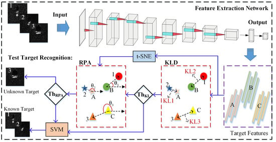
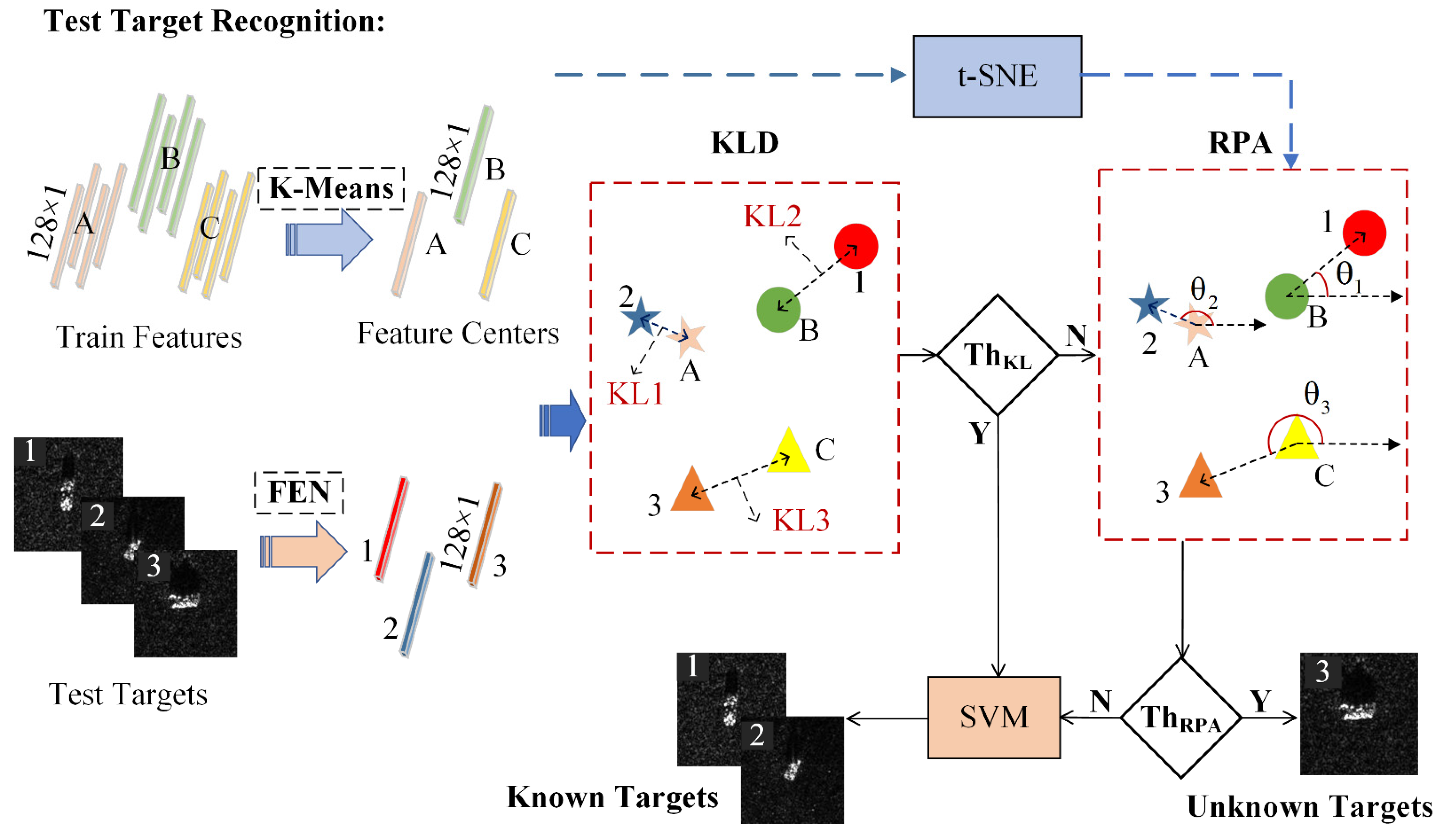
Figure 1 is the overall framework of the Fea-DA unknown SAR target identification method and its specific implementation steps are as follows.
Step1: A 7-layer deep convolutional neural network (DCNN) is built as the FEN of the SAR image target to extract the SAR target features and construct the feature mapping space. After that, the original SAR target image is transformed into a 128 × 1 dimensional feature vector through FEN mapping.
Step2: Performing single category K-Means clustering on the SAR target features of the training set to obtain the target feature centers of all categories.
Step3: When a new target appears, it is first transformed into a 128 × 1 dimensional feature vector via FEN, and the KLD between the feature vector and the feature center of all known training targets is calculated to obtain the similarity measurement between the new target and the known target. Then, the new target is roughly identified by setting an appropriate threshold.
Step4: For the targets that cannot be identified correctly after the rough identification process of the KLD module, their feature vectors perform t-SNE nonlinear dimensionality reduction, thereby mapping the 128-dimensional high dimensional space to the two-dimensional space.
Step5: The RPA is calculated to obtain the relative position angle between the new target and its nearest feature center. By setting an appropriate threshold value, the new target feature is reanalyzed to discriminate its category. If the discriminated result is an unknown target, the target is marked to alert relevant technical staff for further processing and judging. Otherwise, if it is a known target in the library, it is sent to the support vector machine (SVM) classifier to recognize the specific category information.
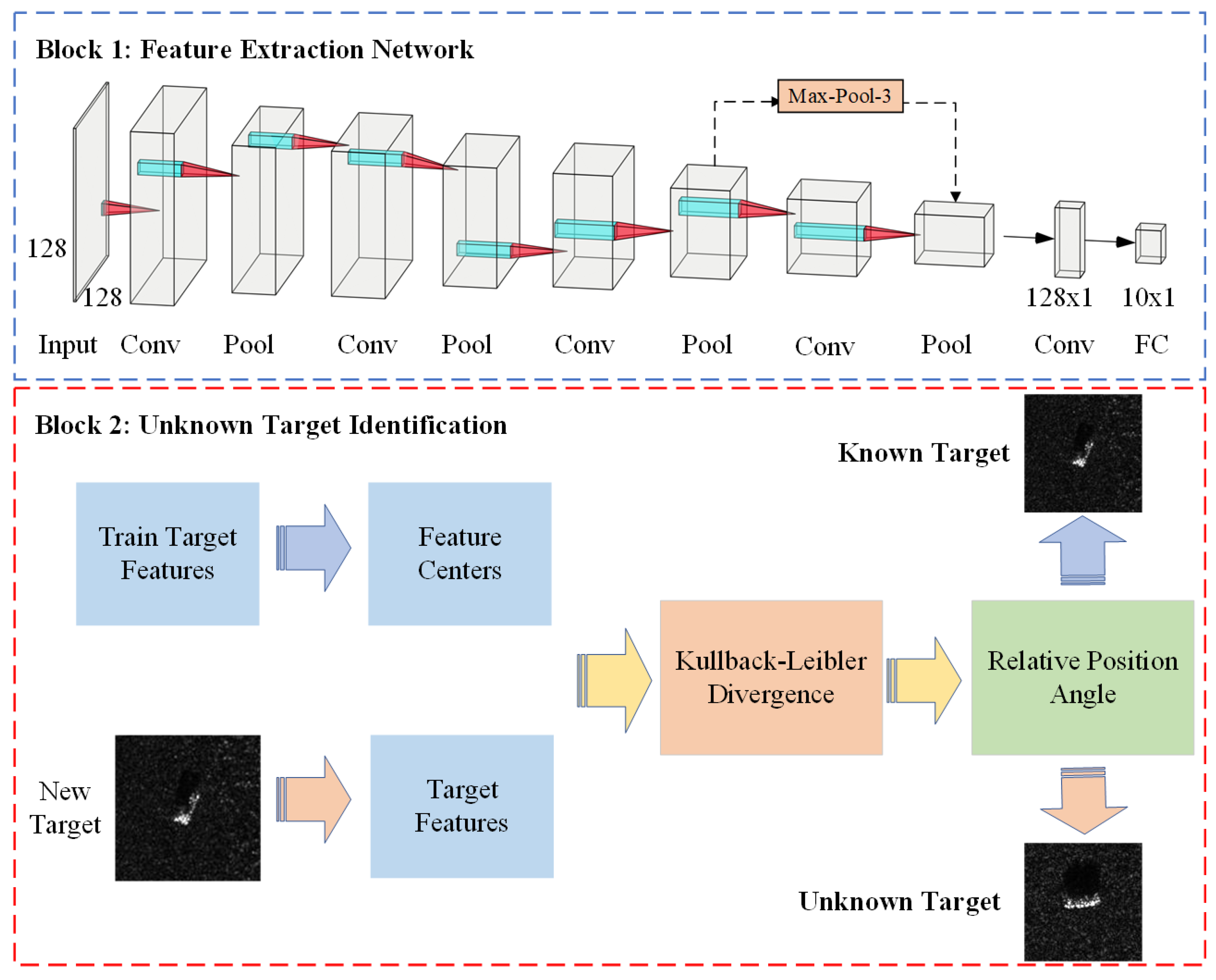
3. Feature Extraction Network
An unknown SAR target identification method relies on a large number of stable and effective SAR target features, and the quality of target features directly affects the recognition performance of SAR targets [9,25,34]. Figure 2 displays the general architecture of FEN, and the network configuration of FEN is listed in Table 1. The backbone network is a seven-layer DCNN, including one input layer, five convolutional layers, and one full connection layer. In particular, each convolution layer consists of convolution, batch normalization (BN), ReLU activation, and maximum pooling (Max-Pooling) operations. For example, in the first convolutional layer, the original SAR target image, with an input size of 128 × 128, is computed by a 20 − 5 × 5 convolution kernel to obtain a 20 − 124 × 124 feature map, and no zero-padding operations. Next, the feature map is converted into a 20 − 62 × 62 feature map through BN, ReLU activation and 2 × 2 Max-Pooling operations in sequence. Note that except for minor changes in the size of the convolution kernel, the subsequent calculation process of the convolution layer is consistent with the above steps. During training, FEN uses cross entropy loss function (CEL) and the Adam optimization algorithm to update the parameters. The CEL is defined as:
where , N is the number of all training samples, is the true value of the i-th sample and represents the output of the model.
3.1. Multiscale Features
In the FEN training process, there is a wealth of multiscale information between the target features of different convolutional layers. Making full use of this feature information can effectively improve the learning ability on the SAR targets. In order to enhance the use of multiscale features by FEN, an effective method is to add skip connection units (SCU) between different convolutional layers [35,36,37]. As shown in Figure 2, after the output of the third convolutional layer of FEN, a 3 × 3 Max-Pooling operation is employed to down sample the 60 − 12 × 12 feature map to a 60 − 4 × 4 feature map. Then, the 60 − 4 × 4 feature map is directly merged with the output of the fourth convolutional layer, the 120 − 4 × 4 feature map, into a 180 − 4 × 4 feature map. Finally, the feature map is transformed into a 128 × 1 feature vector by a 128 − 4 × 4 convolution kernel calculation, and input into the full connection layer.
The SCU mainly has the following two advantages: on the one hand, the SCU can effectively utilize the feature map information of different convolutional layers, and preserve more multiscale features. On the other hand, SCU can alleviate the problems of slow parameter update and vanishing gradient, making the training of FEN smoother. The reason for this is that in the process of parameter backpropagation, the parameter gradient of the lower layer decreases dramatically with the increase in network layers, which will result in the network parameters updating slower. In the worst case, even vanishing gradients may occur, causing the inability of the network model to properly train.
3.2. SVM Classifier
The conventional deep learning model uses the full connection layer + softmax as the classifier. However, this type of structure may fall into a local optimal solution during the parameter update process, and superabundant fully connected layers may also cause over fitting problems and poor generalization performance. Therefore, in FEN, a fully connected layer + softmax feature classifier firstly pretrains the target sample. Then, the feature vector (128 × 1) output by the last convolutional layer is input to the SVM for nonlinear classification when the training is completed. In order to achieve nonlinear classification, the SVM of the nonlinear kernel method is used to map the nonlinear features of the SAR target to a high dimensional space and find a hyperplane in the space that can distinguish the target features. In Fea-DA, the SVM classifier adopts an RBF nonlinear kernel and mainly has the following two functions: a) Participating in the construction of FEN as a nonlinear feature classifier during training. b) In the phase of unknown SAR targets identification, SVM serves as the known target classifier in the library to further finely classify the test target and determine its category when a test target is predicted to be the known target.
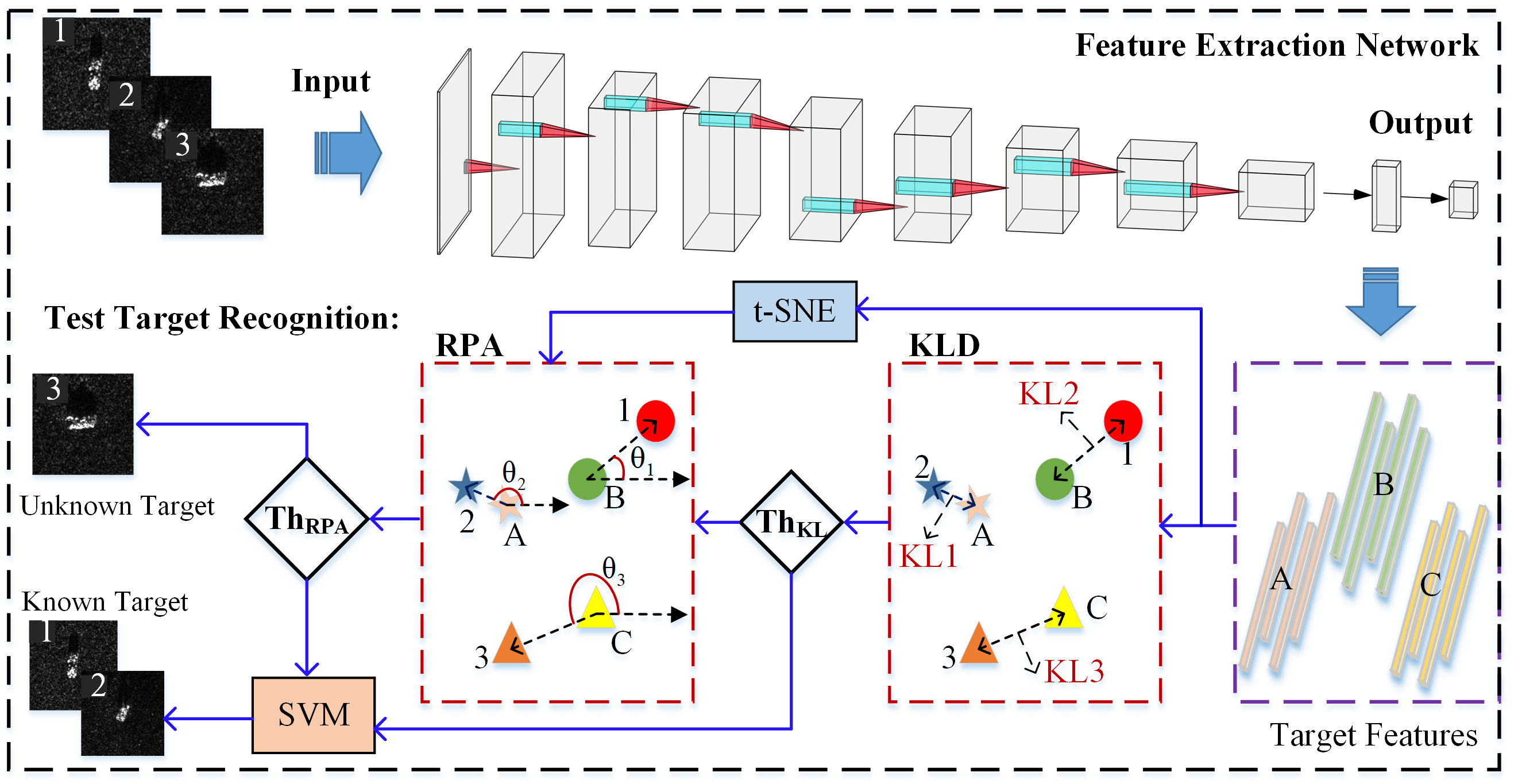
4. KLD-RPA Joint Discrimination
In the procedure of identifying an unknown SAR target, traditional feature subspace mapping discrimination methods have low recognition accuracy due to the absence of analysis and processing of the target features. Therefore, this section proposes a KLD–RPA unknown SAR target identification algorithm based on target feature analysis and joint discriminant to achieve the accurate identification of unknown targets. The proposed algorithm principle is shown in Figure 3. First of all, the SAR target image is converted into a 128 × 1 dimensional feature vector by FEN. Subsequently, all the targets of each category in the training set are individually calculated by the K-Means clustering algorithm to obtain a stable and reliable target category center, and the above steps are repeated to acquire all known target category centers. In the testing phase, the KLD between the feature vector of the test target and the category feature center of the known target is calculated to obtain the similarity between the test target and the known target. Afterwards, the test target category is roughly identified by setting an appropriate threshold. For the targets that cannot be distinguished by KLD, firstly, t-SNE nonlinear dimensionality reduction is performed, and the target features are mapped from high dimensional space to two-dimensional plane space. Then, the RPA between the test target and the nearest known target category center is estimated. Finally, the test target is finely identified through RPA. If the test target is a known target, it is input into the SVM classifier for further classification, otherwise it is marked as an unknown target.
4.1. KL Divergence Discrimination
KLD, also known as relative entropy, information divergence, etc., is a measurement method to evaluate the matching degree between two random distributions, p and q [38,39]. While the two random distributions are similar, the KLD tends to zero. Otherwise, their KLD will also increase as the difference between the two random distributions becomes larger. Therefore, KLD is a non-negative function:
where p is the target distribution, and q is the real distribution. In addition, KLD is an asymmetric similarity measurement function, that is
where p represents the feature distribution of the category center of the known target in the library, q denotes the feature distribution of the test target, and their feature distributions are both 128 × 1 dimensional vector. Hence, the KLD between q and p is defined as:
where and represent the value of the i-th element in the feature distributions p and q, respectively. Therefore, the KLD value distribution between the test target and the known target in the library can be obtained according to Equation (4). At this point, the rough identification of the test target is achieved by setting an appropriate threshold, that is, the test target belongs to a known target or an unknown target. For the known targets, it is fed into the SVM classifier to determine the specific target category. Otherwise, the RPA module is adopted for further fine identification.
4.2. t-SNE Dimensionality Reduction and Visualization Technology
Before performing RPA identification, it is necessary to reduce the dimensionality of the high dimensional target feature vector for the aim of facilitating angle calculation and visualization. The technique of t-SNE is an unsupervised dimensionality reduction method with stable mapping space. The target features after t-SNE dimensionality reduction have the advantages of lower computational cost, excellent visualization, and easy understanding, etc. [40,41]. The main idea of t-SNE is to convert the distance among data points in a high dimensional space into a conditional probability that characterizes similarity, that is, data points with identical distances in high dimensional space are supposed to have similar distances in low dimensional space after dimensionality reduction. Thus, t-SNE can well preserve local similarity between the SAR target. In t-SNE, the distance between the target features is mapped to the probability distribution through affine transformation: a) For target features in high dimensional space, t-SNE converts the distance between target features into Gaussian distribution probability. If the distance between two target features in the high dimensional space is closer, the probability that they will be nearest neighbors after transformation is larger. Conversely, the farther the distance between the target features, the lower the probability that they will be nearest neighbors. b) For low dimensional target features after dimensionality reduction, the t-distribution is selected as the probability distribution model to transform the distance. Finally, feature dimensionality reduction is achieved by optimizing the similarity between the two distributions. The specific optimization process is as follows:
Assume that a given SAR target feature dataset in a high-dimensional space, where is a 128 × 1 feature vector. If and are two target feature vectors in a high dimensional space, is the center point, and the conditional probability of as its nearest neighbor is:
where is the covariance of Gaussian distribution. For different center points, the corresponding covariance is various. Regarding the setting of , this paper performs the binary search method in [40] to determine. In order to speed up the optimization process and reduce the computational cost, joint probability is introduced to replace conditional probability . However, the joint probability is susceptible to outliers, causing a decrease in the dimensionality reduction performance. To solve the problem of outliers, symmetrical conditional probability is used as the equivalent joint probability [40]. Define the equivalent joint probability distribution of target feature vectors and in high dimensional space:
obviously . The equivalent joint probability is used to guarantee , so that each target feature has a certain degree of contribution to the overall optimization process, and it will neither be infinite, nor tend to zero. Therefore, the low dimensional space data points, and , corresponding to and obey the t-distribution, and its equivalent joint probability distribution is:
where . Theoretically, if the dimensionality reduction result is effective and the local features remain intact, then the target feature distribution before and after the dimensionality reduction should be consistent, . Then, KLD is employed to optimize the deviation between the two distributions, and the objective function is written as:
where P represents the joint probability distribution of the target feature in the high dimensional space, and Q is the joint probability distribution of the target feature in the low-dimensional space. By optimizing the objective function, the target feature distribution after dimensionality reduction can be obtained. If the is smaller, the feature distribution after dimensionality reduction is closer to the feature distribution in the original high dimensional space, which indicates that the reduced data effectively retains the local feature information between the target features. Conversely, if the is larger, it shows that more local feature information is lost and the dimensionality reduction effect is worse. Finally, the gradient descent (GD) method is used to update the objective function and its partial derivative is calculated by:
In order to speed up the iterative process and avoid falling into the local optimal solution, the momentum term update is added to the gradient. The final error update formula is:
where indicates the solution at iteration t, the learning rate, and the momentum at iteration t + 1.
With the above optimization solution, t-SNE can map the SAR target feature vector in the high dimensional space to the low dimensional space, especially the two and three dimensionality visualization space. In addition, it can effectively alleviate the “crowding” problem in the feature space, since t-SNE uses Gaussian distribution to convert distance into probability distribution for target features in high dimensional space and utilizes a more heavy tailed t-distribution for target features in low dimensional space, respectively. For target features that are far away, t-SNE will enlarge the distance; for target features that are close to neighbors, t-SNE will shorten the distance. Therefore, t-SNE can effectively preserve the local feature information between neighboring SAR target features.
4.3. Reletive Position Angle Identification
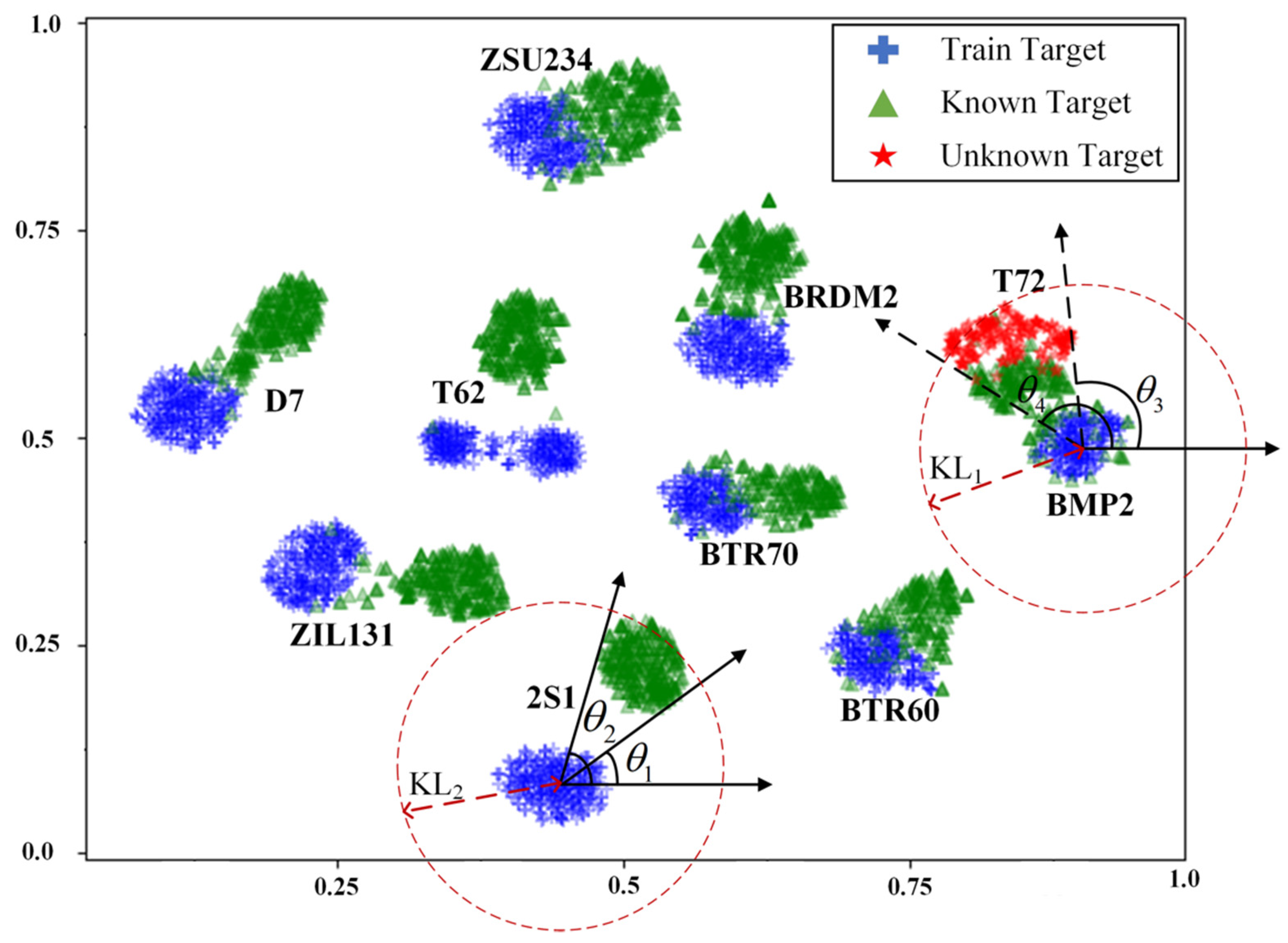
The targets that failed to be identified after rough identification through the KLD module mainly include the following two situations: (1) The test target is a known target, and the KLD value of the target feature diverges due to the inherent difference between the training data and the test data. (2) The test target is an unknown target, which is similar to a certain type or multiple types of targets in the library, leading to a reduction in the KLD value. The above two situations will cause the problem of the KLD numerical aliasing in the target feature space, resulting in a decrease in the unknown SAR target discrimination capability. For example, in the KLD module in Figure 3, the KLD values between the known targets 1, 2; the unknown target 3; and the category centers A, B, C are KL1, KL2, and KL3, respectively. It can be seen that the KLD values of the known target 1 and the unknown target 3 are close. At this time, using a single KLD discrimination will cause serious target misjudgment. Therefore, on the basis of KLD similarity discrimination, Fea-DA adopts RPA [42,43,44] containing target feature angle information to finely identify misjudged targets.
Suppose that the new target is , and represents the collection of known target categories in the library. The category closest to the new target is obtained by KLD similarity calculation:
where denotes the feature center of the known target category .
Assuming a new target feature vector, , and its nearest feature center of the known target, , are mapped to a two-dimensional plane space by t-SNE, and the coordinates after dimensionality reduction are and , respectively. At this point, the RPA of the new target relative to the category is:
The RPA identification process is shown in the RPA module in Figure 3. After the KLD module is roughly identified, the target feature vector is fed into the RPA module to calculate the RPA between the test target and the nearest category according to Equation (12). In Figure 3, the RPAs of the three test targets are , , and . The problem that the known target 1 and the unknown target 3 cannot be distinguished under the KLD measurement, but they can be easily and quickly distinguished under the RPA measurement. From a physical point of view, KLD computes the overall similarity between targets and categories, while RPA characterizes the similarity and differences in similarity between target features in different dimensions. Specifically, KLD calculates the distance between the target feature and the category center, and RPA provides the angle information between them. Eventually, we adopt the joint discrimination of Range–Azimuth to achieve the accurate identification of the unknown target.
In addition, the KLD–RPA unknown SAR target identification algorithm can not only solve the target misjudgment problem in a single KLD similarity measure, but also effectively settle the SCA problem of multiple types of targets that occurs in the traditional absolute angle based similarity measurement method. The traditional absolute cosine angle (ACA) similarity measurement method reflects the correlation of features by calculating the vector angle between the target point and the category center to the origin point. However, when multiple types of targets appear in a certain direction simultaneously, the ACA methods will judge them as the same type of targets, and they cannot be completely distinguished. Different from the traditional methods, the RPA measurement method computes the angle between the new target and the closest known target category center in the library, to obtain the positional relationship of the target. Even if there are multiple types of targets in a certain direction, due to the diverse relative positions between targets and their nearest corresponding categories, the RPA is different. Therefore, the target can be accurately distinguished by calculating the RPA between the targets.
4.4. Threshold Setting
In the KLD–RPA application, the setting of the threshold is extremely crucial for the identification of unknown SAR targets. Here, the prerequisites and basic assumptions for threshold setting are introduced.
4.4.1. KLD Threshold
For the setting of the KLD threshold, the KLD value from the known target in the training set to the center of the corresponding category is first calculated and the maximum KLD value is adopted as the initial threshold. Then, the KLD threshold is controlled by adjusting the threshold coefficient. Assuming that denotes the feature vector of the i-th target in the j-th category of the training set, and the feature center for this type of target is , then the maximum KLD from all targets in the j-th category to the feature center is:
The maximum KLD from the target sample to the center of the corresponding category is:
where M is the target type of the training set. In summary, the KLD threshold is defined as:
where represents the threshold coefficient. The KLD threshold is controlled by changing the threshold coefficient.
4.4.2. RPA Threshold
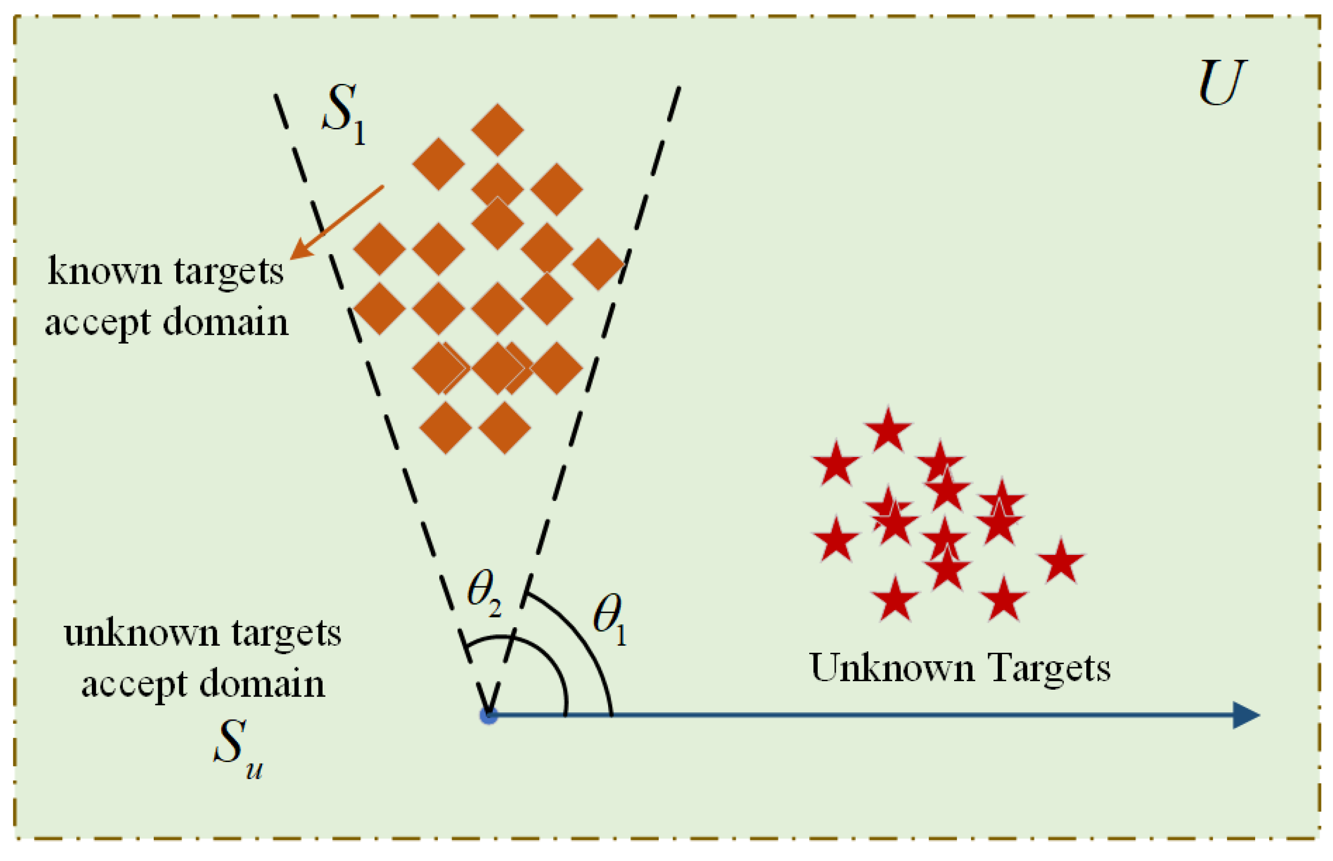
Unknown Target Threshold Decision Strategy (UTTDS): Assume that the accepted domain of the whole targets is U, if the known target accepted domain is S, then the accepted domain of the unknown target is the complementary set of S.
For the setting of the RPA threshold, we employ UTTDS to determine the range of the accepted domain of the unknown target. The specific steps are as follows: First, the target that fails to be successfully distinguished by KLD rough identification is manually identified to determine the specific category of the known target. Then, the RPA of the known targets that have completed the category identification is calculated, and the range of the accepted domain of the known target is determined by analyzing the RPA distribution of the test target. Finally, UTTDS is applied to set the RPA threshold.
Suppose that there is only one type of known targets and unknown targets among the targets that input the RPA identification module, as shown in Figure 4, the overall target accepted domain is , and the known target accepted domain is . Thus, the unknown target accepted domain is:
Therefore, the RPA threshold is:
When there are multiple types of known targets in the target space, assuming that the known target accepted domains are , the corrected RPA threshold is:
5. Experimental Results and Analysis
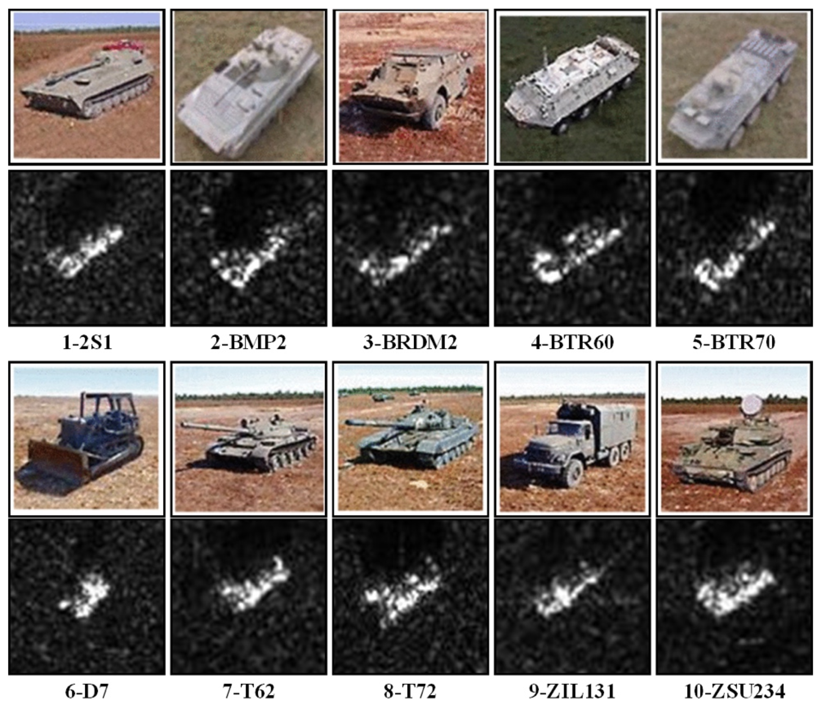
The dataset used in this article is the measured SAR ground stationary target data published by the Moving and Static Target Acquisition and Recognition (MSTAR) program supported by the Defense Advanced Research Projects Agency (DARPA), abbreviated as MSTAR dataset [9,15,19,30]. The dataset employs spotlight high resolution synthetic aperture radar, 0.3 m×0.3 m resolution, X-band, and HH polarization. The MSTAR dataset contains a recommended dataset—MSTAR Public Targets Chips, MPTC, and another mixed target dataset: MSTAR-Public Mixed Targets, MPMT. Among them, the MPTC dataset mainly includes Armored Personnel Carrier–BTR70, Infantry Fighting Vehicle–BMP2, Tank– T72 three types of targets, referred to as 3-type dataset. MPMT dataset contains Self-propelled Artillery–2S1, Amphibious Armored Scout Car–BRDM2, Armored Personnel Carrier–BTR60, Bulldozer–D7, Tank–T62, Truck–ZIL131, Self-propelled Anti-aircraft Gun–ZSU234 seven types of targets. In this experiment, the MPTC and MPMT datasets are combined to form a mixed dataset containing 10 types of targets, named 10 types of dataset. The depression angle of the training set of the 10 types of dataset is 17°, 2747 target samples. And the test set is 15° depression angle, 2425 target samples. Each type of specific sample number allocation and other information on the MSTAR 10 types of dataset are listed in Table 2, and the optical-SAR image comparison is shown in Figure 5.
The experimental hardware configuration is Intel Core i7-7700 CPU, Nvidia 1080Ti GPU; System and software environment: Win10 (Windows System 10, Microsoft, Redmond, WA, USA), Python 3.7 (Python Software Foundation, Wilmington, DE, USA), CUDA 10.1 (Nvidia-USA, Santa Clara, CA, USA), PyTorch 1.6. The experimental results and analysis mainly include FEN performance test and Fea-DA (Facebook-USA, Menlo Park, CA, USA) unknown SAR target identification performance test. The dataset allocation used in the experiment is listed in Table 3.
5.1. The Learning Ability of FEN
5.1.1. Test Error
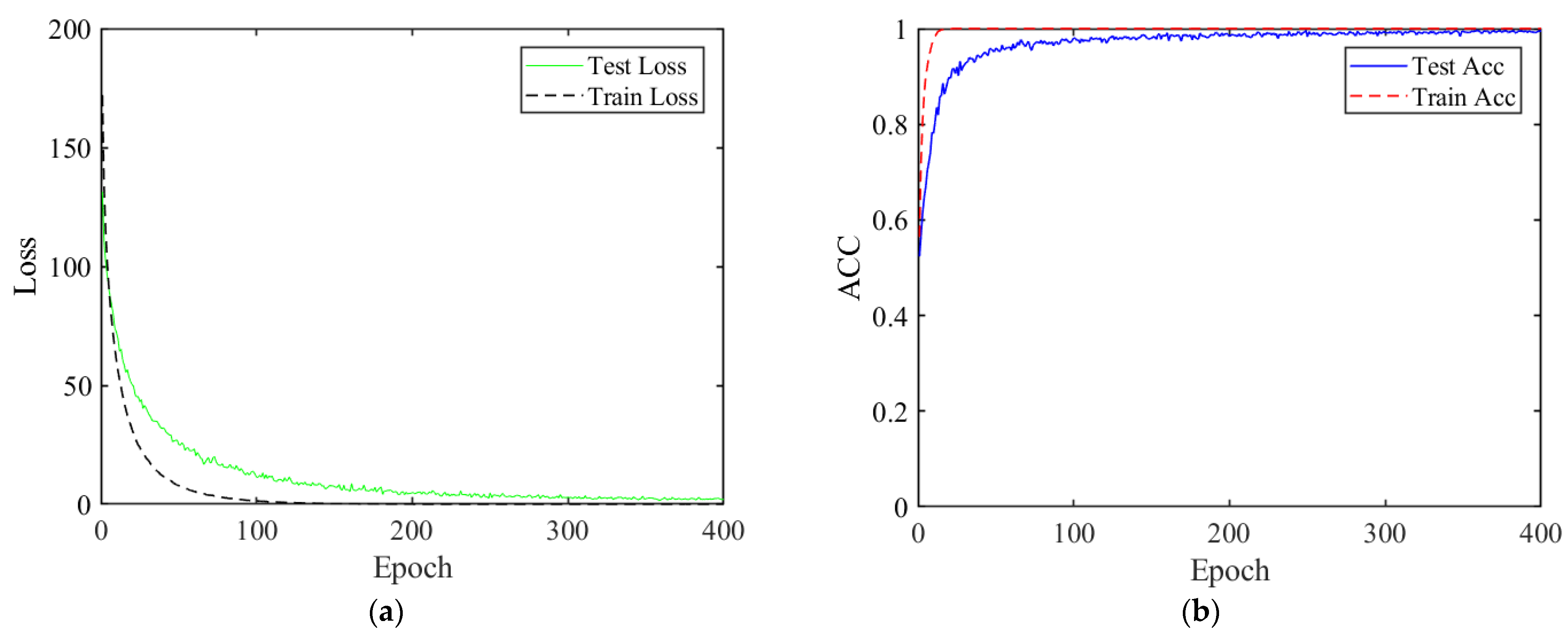
This experiment mainly analyzes and tests the learning ability of the FEN model. Figure 6a shows the train–test error curve of FEN on the 10-type dataset. It can be seen that the training error and the testing error rapidly converge and decrease, and eventually approach to zero with the increase of epoch. Meanwhile, the accuracy of the training set and the testing set also rise speedily and reach to a peak, as illustrated in Figure 6b. This indicates that FEN has a strong learning ability and can effectively approximate the data characteristics of the target sample in the training set. In addition, through the learning of universal features in the target samples of the training set, the target samples of the testing set can be accurately recognized.
5.1.2. Test Accuracy
This experiment mainly conducts statistical and comparative analysis on the test accuracy of FEN. To more intuitively reflect the performance superiority of the proposed FEN model, five classical and state of the art SAR target recognition models are adopted for comparison: A-ConvNets [9], TL-SD [45], KLSF [46], M-PMC [47] and L1-2-CCNN [48]. Table 4 lists the test accuracy of FEN and the other five comparison models on the MSTAR 3-type dataset and 10-type dataset. As the Table shows, in the 3-type datasets the six models have achieved FEN-100%, A-ConvNets-99.49%, TL-SD-99.66%, L1-2-CCNN-99.33%, and M-PMC-98.83%, KLSF-89.1% on recognition accuracy. In addition, in the 10-type datasets, the test accuracy from high to low is L1-2-CCNN-99.86%, TL-SD-99.64%, FEN-99.63%, A-ConvNets-99.13%, M-PMC-98.81%, KLSF-96.1%. It can be obtained from the experimental results that the proposed FEN has achieved competitive recognition accuracy compared to the other approaches. This demonstrates that FEN can effectively learn the implicit feature representation of an SAR target from the training set, and build a stable and reliable feature space by extracting the universal target features from the original SAR image. Furthermore, FEN’s high efficiency feature extraction capabilities also provide guarantee for the subsequent accurate identification of unknown SAR targets.
5.2. Unknown SAR Target Identification
5.2.1. The 1-Type Unknown Target Test
This section tests and analyzes the performance of the Fea-DA unknown SAR target identification method. In order to test the performance of Fea-DA more comprehensively, this paper conducts two sets of experimental test analysis, namely, a 1-type unknown target experiment and 3-type unknown target experiment. Specifically, the 1-type unknown target experiment means that one category of known target is selected as the unknown target from 10 categories of known targets. During training, unknown targets do not participate in the training at all, and only appear in the test phase after the model training has been completed. Furthermore, in order to compare with the existing optimal method, this experiment selects the 8-T72 as the unknown target, and the remaining nine types of targets as the known target. The experimental results are listed in Table 5: The proposed Fea-DA unknown SAR target identification method has a significant improvement in test accuracy compared to the current optimal EM simulation-ZSL [31], VGG+PCA-ZSL [29] and VGG-ZSL [29] models. Particularly, the known target accuracy, unknown target accuracy, and overall target accuracy of Fea-DA reached 97.58%, 84.69%, and 96.53%, respectively. This is about 6% higher than the EM simulation method in the metric of target recognition accuracy on average.
Table 6 displays the classification confusion matrix of Fea-DA among all test target samples on the 1-type unknown dataset. It can be seen that the Fea-DA unknown SAR target identification method has achieved good results in multiple categories of targets. Only in certain categories did the NA problem caused by the similarity between the targets leads to a decrease in the identification accuracy, for example, BMP2 and BTR60. However, in general, to the best of our knowledge, the proposed Fea-DA method can achieve state of the art accurate identification of unknown targets while maintaining a high recognition accuracy of known targets.
5.2.2. The 3-Type Unknown Target Test
In actual application, the appearance of multiple types of unknown targets simultaneously is often faced. For this, the hybrid identification problem of multiple unknown targets, the model needs to accurately distinguish all unknown targets from known targets among multiple targets. Therefore, this section conducts a 3-type unknown target test to investigate the discrimination performance of Fea-DA in the case of multiple unknown targets. The experiment uses a 3-type unknown target dataset for training and testing, namely, select category 5-BTR70, category 8-T72, and category 10-ZSU234 as unknown targets, and the remaining seven categories of targets as known targets for training modeling. In the test phase, the three types of unknown targets are tested separately, and then the three types of targets are merged together for comprehensive testing. In particular, before the comprehensive test of three types of unknown targets, 100 unknown SAR targets are randomly sampled from each category and combined into a test dataset with a quantity of 300. The test results of the three types of unknown targets are shown in Table 7.
Experimental results indicate that Fea-DA can realize the precise identification of the multiple types of unknown targets. When multiple unknown targets appear, Fea-DA accurately distinguishes the unknown target from the known target through the KLD–RPA joint discriminant algorithm. In the single category unknown target test, Fea-DA achieves excellent recognition results (take the lowest accuracy). Specifically, the known target accuracy is 95.05%, the unknown target accuracy 86.73%, and the overall target accuracy 94.42%. In the comprehensive test of the three types of unknown targets, all three metrics of accuracy have declined to some extent, but still maintained a high target recognition accuracy. The test results are as follows: the known target accuracy is 91.43%, the unknown target accuracy 86.33%, and the overall target accuracy 90.72%. Particularly, the identification performance of unknown targets is only decreased by 0.4%, which demonstrates that Fea-DA’s identification performance for unknown SAR targets is more stable and robust.
6. Discussion
6.1. Feature Subspace Mapping
This section mainly analyzes and discusses the feature subspace mapping, and intuitively understands the core principle of the proposed KLD–RPA unknown SAR target joint discriminant algorithm from the perspective of visualization. Figure 7 shows the subspace distribution of the target feature map after the high dimensional feature vector processed by t-SNE dimensionality reduction and visualization. The experiment uses the 1-type unknown target dataset in Table 3. The blue cross represents the feature distribution of the nine types of training target samples, the green triangle symbolizes the corresponding nine types of test known targets, and the red five pointed star indicates the unknown target-T72.
From the experimental results, it is clear that for most categories of targets, the target features of the training set are similar to those of the testing set, and the Euclidean distance between the features is close. In this case, the unknown target can be distinguished from the known target by the rough identification of the KLD module, such as ZSU234, BTR60, BTR70, BRDM2, etc. However, for some categories, the target features of the training set and the testing set are far apart and the similarity decreases. Moreover, due to the similarity between the unknown target and the known target in the library, the Euclidean distance between the unknown target and the known target is reduced. Consequently, the KLD value of the unknown target and the known target are aliased, that is the KLD numerical aliasing problem, which leads to the serious misjudgment of the model. For example, 2S1, BMP2 and T72, their KLD values KL1 and KL2 are cross aliased. At this time, using a single KLD discrimination cannot distinguish various types of targets at all. Therefore, RPA is introduced to perform fine identification on the targets that the KLD module failed to discriminate successfully, so as to realize the accurate identification of unknown targets and known targets. As shown in Figure 7, the RPA accepted domain of the known target 2S1 and the unknown target T72 are and respectively. It can be inferred that the T72 and 2S1 targets can be easily and effectively distinguished by setting an appropriate RPA threshold according to UTTDS.
Therefore, RPA can not only effectively solve the problem of KLD numerical aliasing between target features, but also be used to alleviate the SCA problem of multiple types of targets existing in traditional absolute angle similarity measurement methods. Moreover, we believe that in other types of data processing, RPA based measurement methods also have significant application prospects. In addition, through the visualized target feature mapping subspace, the position and direction information between different target features can also be easily and intuitively obtained. For example, the unknown target T72 is similar to BMP2 and is located on the right side of BRDM2 and other spatial information. In addition, this spatial information can increase our understanding and further processing of unknown targets.
6.2. The t-SNE Nonlinear Dimensionality Reduction
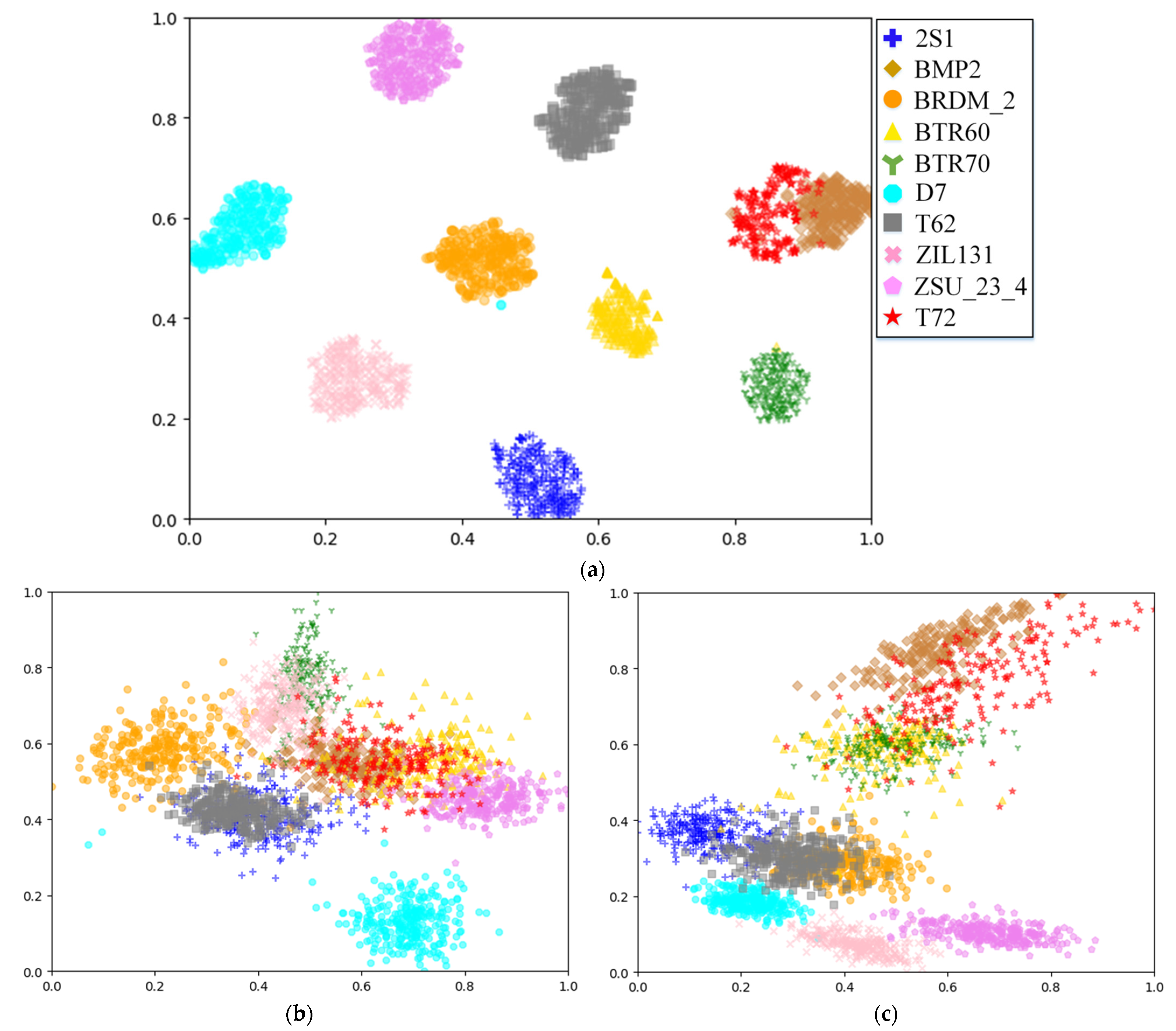
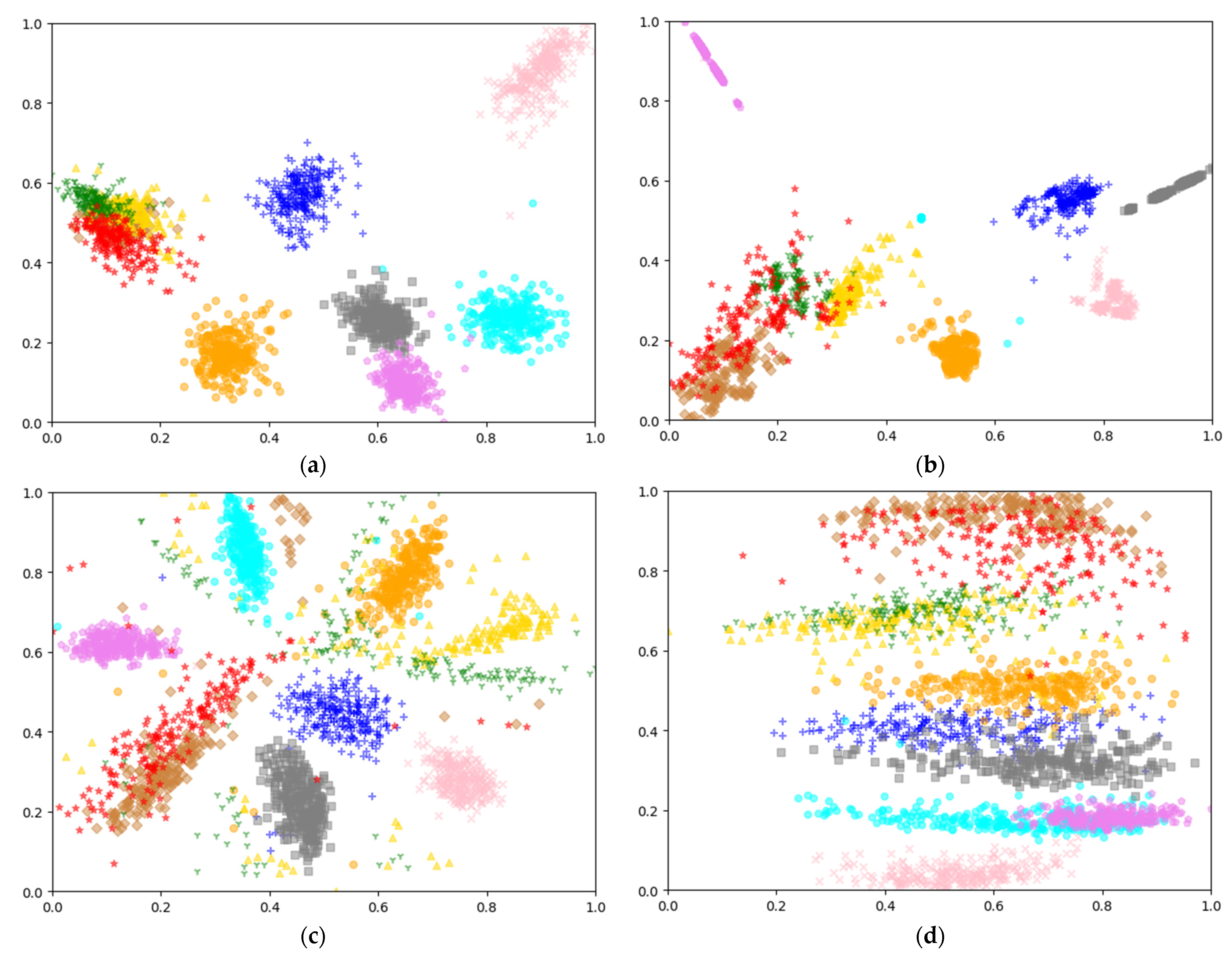
The KLD–RPA joint discrimination algorithm proposed in this paper needs to calculate the relative position angle of the target feature, and then combine with KLD to realize the precise positioning and discrimination of unknown SAR targets. Therefore, it can be inferred that the calculation of RPA directly affects the recognition performance of Fea-DA. In order to facilitate the calculation of the RPA of a target feature, the distribution of targets in the feature space is required to be as compact and scattered as possible, that is, for the same type of targets, the intraclass distance should be as small as possible; for different types of targets, the interclass distance should be as large as possible. Fortunately, t-SNE nonlinear dimensionality reduction technology fits the above characteristics well. The t-SNE transforms the distance between target features in high dimensional space into conditional probability through Gaussian distribution, and employs t-distribution to convert the distance into conditional probability for the target features after dimensionality reduction. For neighboring points, t-SNE will compress the distance; for non-neighboring points, t-SNE will amplify the distance. Therefore, t-SNE can well retain the local characteristics between target features through nonlinear mapping. In order to better reflect the performance of the t-SNE nonlinear dimensionality reduction technology, this section compares and analyzes the six, current mainstream dimensionality reduction methods: random projection (RP), principal component analysis (PCA), linear discriminant analysis (LDA), isometric mapping (ISOMAP), multidimensional scaling (MDS), and totally random trees embedding (TRTE). The experimental results are shown in Figure 8 and Figure 9, respectively.
It can be seen from the experimental results that the dimensionality reduction performance of t-SNE is significantly better than the other six methods. Specifically, results in Figure 8a–c show that the three dimensionality reduction methods of RP, PCA and TRTE have relatively scattered data distribution and a serious overlap problem exists. As indicated in Figure 9a–c, the target feature distribution after LDA, ISOMAP, and MDS dimensionality reduction technology is more compact than the PR, PCA and TRTE methods, but there is still the problem of local target category aliasing. On the contrary, as shown in Figure 8a, the distribution of target features after t-SNE dimensionality reduction is more scattered among different categories, but relatively compact in the same category, and the features are all tightly clustered together. This is because t-SNE is a nonlinear dimensionality reduction technology that converts the distance between data points into conditional probability for the feature distribution, and enables the local feature information of the targets to be well preserved. Namely, t-SNE is capable of compressing the distance between the same type of targets, and enlarging the distance between different categories, which is very conducive to the RPA calculation of target features and also provides a guarantee for the subsequent identification of unknown SAR targets. Therefore, it can be concluded that t-SNE is a nonlinear dimensionality reduction technology with superior performance. However, this does not mean that it is completed once and for all. For example, large amount of calculation, long iteration time, and loss of part of the overall target information still exist. For the use of t-SNE, it needs to be considered according to specific application scenarios and task requirements.
6.3. Ablation Experiments
Fea-DA uses the KLD–RPA joint discrimination algorithm to accurately calculate the range–azimuth of an unknown target. In order to more intuitively reflect the principle and performance of the proposed Fea-DA unknown SAR target identification method, this section conducts ablation experiments on the Fea-DA model. The specific test experiments are as follows: (a) use KLD discrimination alone; (b) the traditional absolute cosine angle (ACA) is adopted to consider the target position information, called the KLD–ACA discrimination; (c) the proposed RPA measurement method is introduced to overcome the problem of multitarget collinear aliasing, called the KLD–RPA joint discrimination. A 1-type unknown target test and 3-type unknown target test were performed on the above three models. The experimental results are shown in Table 8 and Table 9.
From Table 7, Table 8 and Table 9, it can be seen that the recognition accuracy of SAR targets is not much different between KLD discrimination and KLD–ACA discrimination, and the latter is slightly higher. However, both the KLD model and the KLD–ACA model have relatively low recognition accuracy and poor performance for SAR targets. This is because the above KLD and KLD–ACA methods cannot solve the multitarget aliasing problem existing in the target feature space, which limits its recognition performance. On the contrary, the KLD–RPA joint discrimination algorithm used in Fea-DA adopts the RPA measurement to effectively solve the aliasing problem in the target feature space. Specifically, KLD–RPA utilizes the overall similarity of the target and the similarity difference between different dimensions to construct the range–azimuth information between the targets, and realize the accurate identification of unknown targets. The experimental results can also reflect the effectiveness of the KLD–RPA joint discrimination algorithm. It has achieved a significant improvement in recognition performance compared to the other two methods in the 1-type unknown target test and the 3-type unknown target test. The test results are as follows: known target accuracy of 97.58%, unknown target accuracy of 84.69%, overall target accuracy of 96.53% in the 1-type unknown target test and known target accuracy of 91.43%, unknown target accuracy of 86.33%, and overall target accuracy of 90.72% in the 3-type unknown target test (comprehensive test).
7. Conclusions
This paper proposes an unknown SAR target identification method based on feature extraction network, Kullback–Leibler Divergence and relative position angle joint discrimination, named Fea-DA. Firstly, the SAR target utilizes FEN trained on the limited dataset to extract reliable and effective target features. Then the target features are roughly identified by KLD to realize the simple classification of SAR targets. Next, for the SAR targets that failed to be classified by the KLD rough identification, the t-SNE nonlinear dimensionality reduction is performed to convert the high dimensional target feature into the two-dimensional plane space. After that, the target features are processed to calculate the RPA. Finally, the KLD–RPA joint discriminant algorithm is used to accurately identify unknown SAR targets. For the known targets, a trained SVM classifier is employed to finely recognize its category. Experimental results on the MSTAR dataset show that the Fea-DA unknown SAR target identification method can achieve state of the art unknown target identification accuracy. Specifically, the experimental results of 1-type unknown targets are: the known target accuracy of 97.58%, the unknown target accuracy of 84.69%, the overall target accuracy of 96.53%; and the 3-type unknown target comprehensive test results are: the known target accuracy of 91.43%, the unknown target accuracy of 86.33%, and the overall target accuracy of 90.72%. In general, it can be concluded that the proposed Fea-DA unknown SAR target joint discriminant method can achieve the high precision recognition of the unknown target and the known target simultaneously, and possess a satisfactory comprehensive recognition performance. The future research work includes but is not limited to: (1) a more intelligent, prior knowledge driven automatic threshold setting method to improve Fea-DA’s recognition performance for SAR targets, (2) rapid and accurate identification algorithms under the condition of multiple types of unknown targets, (3) calculation method of SAR target RPA measurement in high-dimensional space.
Author Contributions
Z.Z. and J.S. conceived and designed this study. Z.Z. and C.X. performed software and experiments. Z.Z. and H.W. wrote the original manuscript. J.S. and C.X. reviewed and revised the paper. All authors have read and agreed to the published version of the manuscript.
Funding
This research was funded by National Natural Science Foundation of China, grant number 62073334.
Data Availability Statement
This paper adopts the public MSTAR dataset, which is available for all researchers on the official website.
Acknowledgments
The authors would like to thank Zhu Han for assistance in writing and methodology. The source code of this project is uploaded to GitHub: https://github.com/Crush0416/Fea-DA---Unknown-SAR-Target-Identification (accessed on 22 July 2021).
Conflicts of Interest
The authors declare no conflict of interest.
References
- Wang, Z.; Fu, X.; Xia, K. Target Classification for Single-Channel SAR Images Based on Transfer Learning with Subaperture Decomposition. IEEE Geosci. Remote Sens. Lett. 2020, 1–5. [Google Scholar] [CrossRef]
- Wang, L.; Bai, X.; Zhou, F. SAR ATR of Ground Vehicles Based on ESENet. Remote Sens. 2019, 11, 1316. [Google Scholar] [CrossRef] [Green Version]
- Wagner, S. Combination of convolutional feature extraction and support vector machines for radar ATR. In Proceedings of the 17th International Conference on Information Fusion (FUSION), Salamanca, Spain, 7–10 July 2014; IEEE: Piscataway, NJ, USA, 2014; pp. 1–6. [Google Scholar]
- Belloni, C.; Balleri, A.; Aouf, N.; Le Caillec, J.M.; Merlet, T. Explainability of Deep SAR ATR Through Feature Analysis. IEEE Trans. Aerosp. Electron. Syst. 2020, 57, 659–673. [Google Scholar] [CrossRef]
- El Housseini, A.; Toumi, A.; Khenchaf, A. Deep Learning for target recognition from SAR images. In Proceedings of the 2017 Seminar on Detection Systems Architectures and Technologies (DAT), Algiers, Algeria, 20–22 February 2017; IEEE: Piscataway, NJ, USA, 2017; pp. 1–5. [Google Scholar]
- Wang, C.; Pei, J.; Wang, Z.; Huang, Y.; Wu, J.; Yang, H.; Yang, J. When Deep Learning Meets Multi-Task Learning in SAR ATR: Simultaneous Target Recognition and Segmentation. Remote Sens. 2020, 12, 3863. [Google Scholar] [CrossRef]
- Wang, H.; Chen, S.; Xu, F.; Jin, Y.Q. Application of deep-learning algorithms to MSTAR data. In Proceedings of the 2015 IEEE International Geoscience and Remote Sensing Symposium (IGARSS), Milan, Italy, 26–31 July 2015; IEEE: Piscataway, NJ, USA, 2015; pp. 3743–3745. [Google Scholar]
- Wang, Z.; Wang, C.; Pei, J.; Huang, Y.; Zhang, Y.; Yang, H. A Deformable Convolution Neural Network for SAR ATR. In Proceedings of the IGARSS 2020-2020 IEEE International Geoscience and Remote Sensing Symposium, Waikoloa, HI, USA, 26 September–2 October 2020; IEEE: Piscataway, NJ, USA, 2020; pp. 2639–2642. [Google Scholar]
- Chen, S.; Wang, H.; Xu, F.; Jin, Y.Q. Target classification using the deep convolutional networks for SAR images. IEEE Trans. Geosci. Remote. Sens. 2016, 54, 4806–4817. [Google Scholar] [CrossRef]
- Clemente, C.; Pallotta, L.; Gaglione, D.; Maio, A.D.; Soraghan, J.J. Automatic Target Recognition of Military Vehicles with Krawtchouk Moments. IEEE Trans. Aerosp. Electron. Syst. 2017, 53, 493–500. [Google Scholar] [CrossRef] [Green Version]
- Zhao, P.; Liu, K.; Zou, H.; Zhen, X. Multi-Stream Convolutional Neural Network for SAR Automatic Target Recognition. Remote Sens. 2018, 10, 1473. [Google Scholar] [CrossRef] [Green Version]
- Zhou, F.; Wang, L.; Bai, X.; Hui, Y. SAR ATR of ground vehicles based on LM-BN-CNN. IEEE Trans. Geosci. Remote Sens. 2018, 56, 7282–7293. [Google Scholar] [CrossRef]
- Zhang, W.; Zhu, Y.; Fu, Q. Semi-supervised deep transfer learning-based on adversarial feature learning for label limited SAR target recognition. IEEE Access 2019, 7, 152412–152420. [Google Scholar] [CrossRef]
- Zhang, F.; Wang, Y.; Ni, J.; Zhou, Y.; Hu, W. SAR target small sample recognition based on CNN cascaded features and AdaBoost rotation forest. IEEE Geosci. Remote Sens. Lett. 2019, 17, 1008–1012. [Google Scholar] [CrossRef]
- Cui, Z.; Dang, S.; Cao, Z.; Wang, S.; Liu, N. SAR Target Recognition in Large Scene Images via Region-Based Convolutional Neural Networks. Remote Sens. 2018, 10, 776. [Google Scholar] [CrossRef] [Green Version]
- Wang, L.; Bai, X.; Gong, C.; Zhou, F. Hybrid Inference Network for Few-Shot SAR Automatic Target Recognition. IEEE Trans. Geosci. Remote Sens. 2021, 1–13. [Google Scholar] [CrossRef]
- Fu, K.; Zhang, T.; Zhang, Y.; Wang, Z.; Sun, X. Few-Shot SAR Target Classification via Metalearning. IEEE Trans. Geosci. Remote Sens. 2021, 1–14. [Google Scholar] [CrossRef]
- Shang, R.; Wang, J.; Jiao, L.; Stolkin, R.; Hou, B.; Li, Y. SAR targets classification based on deep memory convolution neural networks and transfer parameters. IEEE J. Sel. Top. Appl. Earth Obs. Remote Sens. 2018, 11, 2834–2846. [Google Scholar] [CrossRef]
- Song, Q.; Xu, F.; Jin, Y.Q. SAR Image Representation Learning with Adversarial Autoencoder Networks. In Proceedings of the IGARSS 2019-2019 IEEE International Geoscience and Remote Sensing Symposium, Yokohama, Japan, 28 July–2 August 2019; IEEE: Piscataway, NJ, USA, 2019; pp. 9498–9501. [Google Scholar]
- Sun, Y.; Wang, Y.; Liu, H.; Wang, N.; Wang, J. SAR Target Recognition with Limited Training Data Based on Angular Rotation Generative Network. IEEE Geosci. Remote. Sens. Lett. 2019, 17, 1928–1932. [Google Scholar] [CrossRef]
- Palatucci, M.M.; Pomerleau, D.A.; Hinton, G.E.; Mitchell, T. Zero-shot learning with semantic output codes. In Proceedings of the 22nd International Conference on Neural Information Processing Systems, Vancouver, BC, Canada, 7–10 December 2009; Curran Associates Inc.: Red Hook, NY, USA, 2009; pp. 1410–1418. [Google Scholar]
- Lampert, C.H.; Nickisch, H.; Harmeling, S. Attribute-based classification for zero-shot visual object categorization. IEEE Trans. Pattern Anal. Mach. Intell. 2013, 36, 453–465. [Google Scholar] [CrossRef]
- Suzuki, M.; Sato, H.; Oyama, S.; Kurihara, M. Transfer learning based on the observation probability of each attribute. In Proceedings of the 2014 IEEE International Conference on Systems, Man, and Cybernetics (SMC), San Diego, CA, USA, 5–8 October 2014; IEEE: Piscataway, NJ, USA, 2014; pp. 3627–3631. [Google Scholar]
- Socher, R.; Ganjoo, M.; Sridhar, H.; Bastani, O.; Manning, C.D.; Ng, A.Y. Zero-shot learning through cross-modal transfer. In Proceedings of the Advances in Neural Information, Processing Systems, Lake Tahoe, NV, USA, 5–10 December 2013; MIT Press: Cambridge, MA, USA, 2013; pp. 935–943. [Google Scholar]
- Zhang, L.; Xiang, T.; Gong, S. Learning a deep embedding model for zero-shot learning. In Proceedings of the IEEE Conference on Computer Vision and Pattern Recognition, Honolulu, HI, USA, 21–26 July 2017; pp. 2021–2030. [Google Scholar]
- Pradhan, B.; Al-Najjar, H.A.H.; Sameen, M.I.; Tsang, I.; Alamri, A.M. Unseen Land Cover Classification from High-Resolution Orthophotos Using Integration of Zero-Shot Learning and Convolutional Neural Networks. Remote Sens. 2020, 12, 1676. [Google Scholar] [CrossRef]
- Wei, Q.R.; He, H.; Zhao, Y.; Li, J.A. Learn to Recognize Unknown SAR Targets from Reflection Similarity. IEEE Geosci. Remote Sens. Lett. 2020, 1–5. [Google Scholar] [CrossRef]
- Changpinyo, S.; Chao, W.-L.; Gong, B.; Sha, F. Synthesized classifiers for zero-shot learning. In Proceedings of the IEEE Conference on Computer Vision and Pattern Recognition, Las Vegas, NV, USA, 27–30 June 2016; pp. 5327–5336. [Google Scholar]
- Toizumi, T.; Sagi, K.; Senda, Y. Automatic association between sar and optical images based on zero-shot learning. In Proceedings of the IGARSS 2018-2018 IEEE International Geoscience and Remote Sensing Symposium, Valencia, Spain, 22–27 July 2018; IEEE: Piscataway, NJ, USA, 2018; pp. 17–20. [Google Scholar]
- Song, Q.; Xu, F. Zero-shot learning of SAR target feature space with deep generative neural networks. IEEE Geosci. Remote Sens. Lett. 2017, 14, 2245–2249. [Google Scholar] [CrossRef]
- Song, Q.; Chen, H.; Xu, F.; Cui, T.J. EM Simulation-Aided Zero-Shot Learning for SAR Automatic Target Recognition. IEEE Geosci. Remote Sens. Lett. 2019, 17, 1092–1096. [Google Scholar] [CrossRef]
- Serafino, F.; Lugni, C.; Nieto Borge, J.C.; Soldovieri, F. A Simple Strategy to Mitigate the Aliasing Effect in X-band Marine Radar Data: Numerical Results for a 2D Case. Sensors 2011, 11, 1009–1027. [Google Scholar] [CrossRef] [Green Version]
- Seo, K.W.; Wilson, C.R.; Chen, J.; Waliser, D.E. GRACE’s spatial aliasing error. Geophys. J. Int. 2008, 172, 41–48. [Google Scholar] [CrossRef] [Green Version]
- Ayinde, B.; Inanc, T.; Zurada, J. Regularizing Deep Neural Networks by Enhancing Diversity in Feature Extraction. IEEE Trans. Neural Netw. Learn. Syst. 2019, 30, 2650–2661. [Google Scholar] [CrossRef]
- Li, X.; Zhao, L.; Wei, L.; Yang, M.-H.; Wu, F.; Zhuang, Y.; Ling, H.; Wang, J. Deepsaliency: Multi-task deep neural network model for salient object detection. IEEE Trans. Image Process. 2016, 25, 3919–3930. [Google Scholar] [CrossRef] [Green Version]
- Zhang, X.; Li, B.; Hu, H. Scale-aware hierarchical loss: A multipath RPN for multi-scale pedestrian detection. In Proceedings of the 2017 IEEE Visual Communications and Image Processing (VCIP), St. Petersburg, FL, USA, 10–13 December 2017; IEEE: Piscataway, NJ, USA, 2017; pp. 1–4. [Google Scholar]
- Jiang, H.; Zhang, C.; Wu, M. Pedestrian detection based on multi-scale fusion features. In Proceedings of the 2018 International Conference on Network Infrastructure and Digital Content (IC-NIDC), Guiyang, China, 22–28 August 2018; IEEE: Piscataway, NJ, USA, 2018; pp. 329–333. [Google Scholar]
- Goldberger, J.; Gordon, S.; Greenspan, H. An Efficient Image Similarity Measure Based on Approximations of KL-Divergence Between Two Gaussian Mixtures. In Proceedings of the International Conference on Computer Vision (ICCV), Nice, France, 13–16 October 2003; Volume 3, pp. 487–493. [Google Scholar]
- Pan, J.S.; Weng, C.Y.; Wu, M.E.; Chen, C.Y.; Chen, C.M.; Tsai, C.S. A KL Divergence Function for Randomized Secret Shares. In Proceedings of the 2015 International Conference on Intelligent Information Hiding and Multimedia Signal Processing (IIH-MSP), Adelaide, SA, Australia, 23–25 September 2015; IEEE: Piscataway, NJ, USA, 2015; pp. 231–234. [Google Scholar]
- Laurens, V.D.M.; Hinton, G. Visualizing data using t-SNE. J. Mach. Learn. Res. 2008, 9, 2579–2605. [Google Scholar]
- Pan, M.; Jiang, J.; Kong, Q.; Shi, J.; Sheng, Q.; Zhou, T. Radar HRRP target recognition based on t-SNE segmentation and discriminant deep belief network. IEEE Geosci. Remote Sens. Lett. 2017, 14, 1609–1613. [Google Scholar] [CrossRef]
- Hlavacs, H.; Hummel, K. Cooperative Positioning when Using Local Position Information: Theoretical Framework and Error Analysis. IEEE Trans. Mob. Comput. 2013, 12, 2091–2104. [Google Scholar] [CrossRef]
- Jiang, W.; Liu, Y.; Cai, B.; Rizos, C.; Wang, J.; Jiang, Y. A New Train Integrity Resolution Method Based on Online Carrier Phase Relative Positioning. IEEE Trans. Veh. Technol. 2020, 69, 10519–10530. [Google Scholar] [CrossRef]
- Raut, Y.; Katkar, V.; Sarode, S. Early alert system using relative positioning in Vehicular Ad-hoc Network. In Proceedings of the 2014 Annual International Conference on Emerging Research Areas: Magnetics, Machines and Drives (AICERA/iCMMD), Kerala, India, 24–26 July 2014; pp. 1–8. [Google Scholar]
- Wang, C.; Shi, J.; Zhou, Y.; Yang, X.; Zhou, Z.; Wei, S.; Zhang, X. Semisupervised Learning-Based SAR ATR via Self-Consistent Augmentation. IEEE Trans. Geosci. Remote Sens. 2020, 1–12. [Google Scholar] [CrossRef]
- Dong, G.; Kuang, G. Target Recognition in SAR Images via Classification on Riemannian Manifolds. IEEE Geosci. Remote Sens. Lett. 2015, 12, 199–203. [Google Scholar] [CrossRef]
- Park, J.; Kim, K. Modified polar mapping classifier for SAR automatic target recognition. IEEE Trans. Aerosp. Electron. Syst. 2014, 50, 1092–1107. [Google Scholar] [CrossRef]
- Kechagias-Stamatis, O.; Aouf, N. Fusing Deep Learning and Sparse Coding for SAR ATR. IEEE Trans. Aerosp. Electron. Syst. 2019, 55, 785–797. [Google Scholar] [CrossRef] [Green Version]
Figure 1.
Fea-DA overall framework.

Figure 2.
The architecture of FEN.

Figure 3.
The principle of KLD–RPA joint discriminant algorithm. A, B, and C are known category centers, and target 1, target 2, and target 3 are test targets, among which target 1, 2 are known targets, and target 3 is an unknown target.
Figure 3.
The principle of KLD–RPA joint discriminant algorithm. A, B, and C are known category centers, and target 1, target 2, and target 3 are test targets, among which target 1, 2 are known targets, and target 3 is an unknown target.

Figure 4.
The principle of UTTDS.

Figure 5.
The Optical-SAR image comparison of 10 types of dataset.

Figure 6.
FEN learning ability. (a) Training–testing error curve; (b) Training–testing accuracy curve.
Figure 6.
FEN learning ability. (a) Training–testing error curve; (b) Training–testing accuracy curve.

Figure 7.
SAR target feature mapping subspace distribution after t-SNE visualization processing: the horizontal and vertical axes represent target feature in the two-dimensional space after the t-SNE dimensionality reduction in the high dimensional feature space.
Figure 7.
SAR target feature mapping subspace distribution after t-SNE visualization processing: the horizontal and vertical axes represent target feature in the two-dimensional space after the t-SNE dimensionality reduction in the high dimensional feature space.

Figure 8.
Visualizations of 2425 targets from the Testing Set in 10-type dataset. (a) Visualization by t-SNE; (b) visualization by RP; (c) visualization by PCA. The horizontal and vertical axes represent the target feature in the two-dimensional space after the t-SNE dimensionality reduction in the high dimensional feature space.

Figure 9.
Visualizations of 2425 targets from the Testing Set in 10-type Dataset. (a) Visualization by LDA; (b) visualization by ISOMAP; (c) visualization by MDS; (d) visualization by TRTE. The horizontal and vertical axes represent the target feature in the two-dimensional space after the t-SNE dimensionality reduction in the high dimensional feature space.


Table 1.
The network configuration of FEN.
| Pathway | Layer Composition | Size |
|---|---|---|
| Input Layer | - | 1 − 128 × 128 |
| Conv Layer1 | Conv-20-5 × 5 BN ReLU Max-Pooling-2 | 20 − 62 × 62 |
| Conv Layer2 | Conv-40-5 × 5 BN ReLU Max-Pooling-2 | 40 − 29 × 29 |
| Conv Layer3 | Conv-60-6 × 6 BN ReLU Max-Pooling-2 | 60 − 12 × 12 |
| Conv Layer4 | Conv-120-5 × 5 BN ReLU Max-Pooling-2 | 120 − 4 × 4 |
| Conv Layer5 | Conv-128-4 × 4 BN ReLU | 128 − 1 × 1 |
| FC Layer | - | 10 × 1 |
Table 2.
MSTAR 10 types of dataset.
| Categories | Training Set (Depression Angle: 17°) | Testing Set (Depression Angle: 15°) |
|---|---|---|
| 1-2S1 | 299 | 274 |
| 2-BMP2 | 233 | 195 |
| 3-BRDM2 | 298 | 274 |
| 4-BTR60 | 256 | 195 |
| 5-BTR70 | 233 | 196 |
| 6-D7 | 299 | 274 |
| 7-T62 | 299 | 273 |
| 8-T72 | 232 | 196 |
| 9-ZIL131 | 299 | 274 |
| 10-ZSU234 | 299 | 274 |
| Total | 2747 | 2425 |
Table 3.
Experimental datasets configuration.
| Datasets | Known Categories | Unknown Categories | Training Set | Testing Set |
|---|---|---|---|---|
| 3-type | 2, 5, 8 | - | 698 | 587 |
| 10-type | 1, 2, 3, 4, 5, 6, 7, 8, 9, 10 | - | 2747 | 2425 |
| 1-type unknown | 1, 2, 3, 4, 5, 6, 7, 9, 10 | 8 | 2515 | 2229 |
| 3-type unknown | 1, 2, 3, 4, 6, 7, 9 | 5, 8, 10 | 1983 | 1759 |
Table 4.
The test accuracy of FEN, A-ConvNets, TL-SD, L1-2-CCNN, M-PMC and KLSF.
| Datasets | Models | ACC |
|---|---|---|
| 3-type | FEN | 100% |
| A-ConvNets | 99.49% | |
| TL-SD | 99.66% | |
| L1-2-CCNN | 99.33% | |
| M-PMC | 98.83% | |
| KLSF | 89.1% | |
| 10-type | FEN | 99.63% |
| A-ConvNets | 99.13% | |
| TL-SD | 99.64% | |
| L1-2-CCNN | 99.86% | |
| M-PMC | 98.81% | |
| KLSF | 96.1% |
Table 5.
Results of 1-type unknown target test.
| Models | Known Target Accuracy | Unknown Target Accuracy | Overall Target Accuracy |
|---|---|---|---|
| Fea-DA | 97.58% | 84.69% | 96.53% |
| EM simulation-ZSL | 91.93% | 79.08% | 88.01% |
| VGG+PCA-ZSL | 84.07% | 71.42% | 83.05% |
| VGG-ZSL | 67.83% | 57.14% | 66.97% |
Table 6.
T72 confusion matrix.
| Category | 2S1 | BMP2 | BRDM2 | BTR60 | BTR70 | D7 | T62 | ZIL131 | ZSU234 | T72 |
|---|---|---|---|---|---|---|---|---|---|---|
| 2S1 | 270 | 0 | 0 | 0 | 0 | 0 | 1 | 2 | 1 | 0 |
| BMP2 | 0 | 154 | 0 | 0 | 0 | 0 | 0 | 0 | 0 | 41 |
| BRDM2 | 0 | 0 | 274 | 0 | 0 | 0 | 0 | 0 | 0 | 0 |
| BTR60 | 0 | 0 | 0 | 195 | 0 | 0 | 0 | 0 | 0 | 0 |
| BTR70 | 0 | 0 | 0 | 0 | 186 | 0 | 0 | 0 | 0 | 10 |
| D7 | 0 | 0 | 2 | 0 | 0 | 272 | 0 | 0 | 0 | 0 |
| T62 | 0 | 0 | 0 | 0 | 0 | 0 | 271 | 0 | 2 | 0 |
| ZIL131 | 0 | 0 | 0 | 0 | 0 | 0 | 0 | 273 | 1 | 0 |
| ZSU234 | 0 | 0 | 0 | 0 | 0 | 0 | 0 | 0 | 272 | 2 |
| T72 | 0 | 23 | 0 | 7 | 0 | 0 | 0 | 0 | 0 | 166 |
Table 7.
Results of 3-type unknown target test.
| Model | Unknown Category | Known Target Accuracy | Unknown Target Accuracy | Overall Target Accuracy |
|---|---|---|---|---|
| Fea-DA | 5 | 95.62% | 86.73% | 94.73% |
| 8 | 95.05% | 88.78% | 94.42% | |
| 10 | 97.56% | 97.44% | 97.54% | |
| 5, 8, 10 | 91.43% | 86.33% | 90.72% |
Table 8.
Results of 1-type unknown target test on Fea-DA, KLD-ACA and KLD models.
| Models | Known Target Accuracy | Unknown Target Accuracy | Overall Target Accuracy |
|---|---|---|---|
| Fea-DA | 97.58% | 84.69% | 96.53% |
| KLD-ACA | 82.05% | 81.63% | 82.02% |
| KLD | 80.04% | 81.12% | 80.12% |
Table 9.
Results of 3-type unknown target test on KLD-ACA and KLD models.
| Model | Unknown Category | Known Target Accuracy | Unknown Target Accuracy | Overall Target Accuracy |
|---|---|---|---|---|
| KLD-ACA | 5 | 90.79% | 83.67% | 90.08% |
| 8 | 75.50% | 73.47% | 75.29% | |
| 10 | 94.26% | 93.80% | 94.20% | |
| 5, 8, 10 | 86.36% | 82.00% | 85.72% | |
| KLD | 5 | 92.44% | 82.14% | 91.41% |
| 8 | 75.67% | 73.98% | 75.50% | |
| 10 | 93.63% | 94.89% | 93.80% | |
| 5, 8, 10 | 85.96% | 81.67% | 85.33% |
Publisher’s Note: MDPI stays neutral with regard to jurisdictional claims in published maps and institutional affiliations. |
© 2021 by the authors. Licensee MDPI, Basel, Switzerland. This article is an open access article distributed under the terms and conditions of the Creative Commons Attribution (CC BY) license (https://creativecommons.org/licenses/by/4.0/).
Share and Cite
MDPI and ACS Style
Zeng, Z.; Sun, J.; Xu, C.; Wang, H. Unknown SAR Target Identification Method Based on Feature Extraction Network and KLD–RPA Joint Discrimination. Remote Sens. 2021, 13, 2901. https://0-doi-org.brum.beds.ac.uk/10.3390/rs13152901
AMA Style
Zeng Z, Sun J, Xu C, Wang H. Unknown SAR Target Identification Method Based on Feature Extraction Network and KLD–RPA Joint Discrimination. Remote Sensing. 2021; 13(15):2901. https://0-doi-org.brum.beds.ac.uk/10.3390/rs13152901
Chicago/Turabian StyleZeng, Zhiqiang, Jinping Sun, Congan Xu, and Haiyang Wang. 2021. "Unknown SAR Target Identification Method Based on Feature Extraction Network and KLD–RPA Joint Discrimination" Remote Sensing 13, no. 15: 2901. https://0-doi-org.brum.beds.ac.uk/10.3390/rs13152901
Note that from the first issue of 2016, this journal uses article numbers instead of page numbers. See further details here.