
Deep Hashing Using Proxy Loss on Remote Sensing Image Retrieval


1
School of Computer Science and Technology, Jilin University, Changchun 130012, China
2
Key Laboratory of Symbolic Computation and Knowledge Engineering, Ministry of Education, Jilin University, Changchun 130012, China
3
School of Mechanical Science and Engineering, Jilin University, Changchun 130025, China
4
School of Communication Engineering, Jilin University, Changchun 130012, China
5
School of Computer Science and Technology, Shandong University of Technology, Zibo 255000, China
*
Author to whom correspondence should be addressed.
Remote Sens. 2021, 13(15), 2924; https://0-doi-org.brum.beds.ac.uk/10.3390/rs13152924
Submission received: 15 June 2021
/
Revised: 19 July 2021
/
Accepted: 22 July 2021
/
Published: 25 July 2021
(This article belongs to the Special Issue Theory and Application of Machine Learning in Remote Sensing)
Abstract
:With the improvement of various space-satellite shooting methods, the sources, scenes, and quantities of remote sensing data are also increasing. An effective and fast remote sensing image retrieval method is necessary, and many researchers have conducted a lot of work in this direction. Nevertheless, a fast retrieval method called hashing retrieval is proposed to improve retrieval speed, while maintaining retrieval accuracy and greatly reducing memory space consumption. At the same time, proxy-based metric learning losses can reduce convergence time. Naturally, we present a proxy-based hash retrieval method, called DHPL (Deep Hashing using Proxy Loss), which combines hash code learning with proxy-based metric learning in a convolutional neural network. Specifically, we designed a novel proxy metric learning network, and we used one hash loss function to reduce the quantified losses. For the University of California Merced (UCMD) dataset, DHPL resulted in a mean average precision (mAP) of up to 98.53% on 16 hash bits, 98.83% on 32 hash bits, 99.01% on 48 hash bits, and 99.21% on 64 hash bits. For the aerial image dataset (AID), DHPL achieved an mAP of up to 93.53% on 16 hash bits, 97.36% on 32 hash bits, 98.28% on 48 hash bits, and 98.54% on 64 bits. Our experimental results on UCMD and AID datasets illustrate that DHPL could generate great results compared with other state-of-the-art hash approaches.
1. Introduction
The number of remote sensing images is increasing due to increases in observation and storage capacity [1]. At the same time, remote sensing images have a lot of difficulty being processed because they contain a large number of geographical regions and regional semantic examples [2,3,4,5,6]. Therefore, many image processing studies focus on remote sensing images. Among them, the most common technologies are image recognition, target detection, image classification, retrieval, and so on. In this paper, we explore image retrieval on remote sensing images. The image retrieval task is to return all images similar to the given one. Image retrieval on remote sensing images [7,8,9] mainly focuses on research content. At present, most researchers in image retrieval focus on improving retrieval efficiency and accuracy. This is also the biggest difficulty in the retrieval direction of remote sensing images, because these images include a large range of geographical landmarks and fine-grained content differentiation.
Remote sensing image retrieval (RSIR) [2,3,4,5,6] can improve retrieval effectiveness through deep metric learning (DML). DML uses labeled images as the input for end-to-end network training. Some excellent trained networks can extract representative features from input images so that similar pairs are close to each other on feature space and dissimilar pairs are far from each other on feature space [10,11]. This feature addresses image retrieval’s need to distinguish the different categories of samples. Generally speaking, the cardinal category of DML losses contain two classes: pair-based losses and proxy-based losses. Pair-based losses explore pair-to-pair relationship between samples in the feature space [12,13,14,15,16,17]. Through training, they can maintain the original spatial relationship between samples, so as to achieve a better retrieval effect. However, the retention of this information usually depends heavily on the construction of input sample pairs, and more training samples will consume more training time, resulting in better training effects. The time complexity of this loss is or , where Q represents the number of training samples, thus its convergence is slow during training. At the same time, because the information contained in different samples plays different roles in training, pairwise loss will also involve sampling technology [2,17,18,19,20]. Proxy-based losses use some proxies to make all samples close to their proxy, which define the same class [21,22,23,24]. Each of the proxies is the representation of some input samples which would be updated by the network training. Usually, it pulls input data to be close to the same class proxies, and pulls it to be far from different class proxies. This could solve the problem of the slow convergence of pair-based loss. In this work, we attempt to use the proxy-based loss to resolve the complexity of the training network.
Retrieval tasks involving a large number of RS images will lead to intolerable retrieval times and the consumption of a large amount of physical storage space. It is necessary to solve this problem to obtain high-speed and precise retrieval tasks. Hash technology is a dimension reduction technique: by encoding, it can significantly reduce retrieval speed and memory consumption. Due to its excellent retrieval results, it is being adopted more and more for large data retrieval tasks. The hashing method is to train some nonlinear functions to encode long features into short features. Then low dimensional features will be calculated as binary code. At present, there are two main categories of hash methods: unsupervised hash and supervised hash. An unsupervised hash method is suitable for learning hash functions with no label information, such as spectral hashing (SH) [25], iterative quantization (ITQ) [26], and discrete graph hashing (DGH) [27]. A supervised hash method is suitable for learning hash functions with label information, as it would produce better dimension reduction effects because of the label information. Some classical supervised hash methods include binary reconstruction embedding (BRE) [28], minimal loss hashing (MLH) [29], sparse embedding, least variance encoding (SELVE) [30], and supervised hashing with kernels (KSH) [31]. By using supervisory information, the binary codes of similar images have great similarity, while those of different images have little similarity.
Ordinarily, from the point of view of feature acquisition, there are two hash methods that are available: traditional hashing methods using manual features, and deep hashing methods using deep features. Traditional hashing techniques contain scale invariant feature transformation (SIFT) [32], GIST [33] and so on. These kind of features focus primarily on the sample content, and traditional methods cannot make adjustments for specific tasks flexibility. The feature expression ability of manual feature is limited, and at the same time, they cannot dynamically adjust the features, so it is difficult to meet the common precision requirements of retrieval tasks. In contrast, deep hashing [34,35,36,37,38,39] uses high-dimensional deep features to learn hash code. These methods use deep neural networks to obtain deep features which do not have human interference, and are thus more discriminative and robust. The deep hashing method commits to learn low-dimensional hash code, and the hash code could represent the sample information very well, while at the same time it can complete the retrieval task with a small in-class distance and a large out-class distance. From the perspective of category differentiation, this is consistent with the goal of DML. In general, deep hashing first inputs the samples into a deep neural network to obtain deep embedding features, and then changes the deep embedding features with high dimensional features into low dimensional hash codes in an end-to-end approach. In particular, the training process consists of two parts. First, we need to train the network with one appropriate loss function to obtain more representative features. The second part uses the hash network to learn the low-dimensional features, while using one appropriate quantization loss to reduce the distance between the hash code and the “hash-like codes”. Among them, “hash-like codes” are our shorthand for low-dimensional features that existed before quantification.
Based on the previous analysis, we choose to use the deep metric learning method to learn deep features, and the deep hashing method to learn hash code. In general, we present a new deep metric learning loss: when the proxy-based loss is used, the relationship between sample pairs is also considered. First, we generate a few proxies to be representatives of the different categories of samples. Second, we use these proxies to build our proxy-based losses while taking into account the optimal state information. Then, we use the novel loss named DHPL (deep hashing using proxy loss) and quantitative losses to train our deep neural network and hash network. In the end, we have a network well-trained to perform fast and high-precision hash retrieval operations.
We list the main innovations and results of this paper as follows:
- We devised a novel proxy-based loss to learn more about informative deep features. It not only considers pairwise information to learn more representative embedding sphere distributions, but also considers the difference between the current state and the optimal state.
- We used one full connection layer to construct our deep hash network in order to learn valid hash functions. It used deep embedding features to fully train the network weights, and used hash losses to reduce the resulting damage from quantification.
- Results are verified by experiments on remote sensing datasets UCMD and AID. The experimental data also show that our DHPL method is more effective than other state-of-the-art methods, which verifies the effectiveness of our method.
Next, our article introduces four parts respectively. Section 2 illustrates the relevant work related to deep metric learning and hashing methods. Section 3 describes the implementation ways of our DHPL method, and Section 4 gives the comparative results of the experiment and analyzes the results. Section 5 summarizes the conclusions of our method.
2. Related Work
Deep metric learning is used in embedding spaces with high degrees of learning differentiation, so that the learned features can be distinguished well between different categories. Deep metric learning losses contain two categories: pair-based losses and proxy-based losses. Pair-bases losses study embedding features by exploring the relationships between samples. Contrastive losses [12] explore the distance between the two samples so that pairs from the same class are closer and pairs from different classes are farther away. Triplet losses [13] explore the distance between three samples, made of anchor data, positive data, and negative data. It can keep the measurements between positive and negative sample pairs within the margins. Finally, the distance among samples of the same class is small, and the distance among samples of the different class is large. N-pair loss [15] assigns one positive sample and several negative samples (one from each different category) to each anchor, so as to explore the information between the samples in a more comprehensive way. Lifted structured loss [14] takes into account one similar pair and multiple dissimilar pairs. This structure can better maintain the sample distribution information, allowing for better trained networks. These pair-to-pair losses can take advantage of more comprehensive sample information by using as many samples as possible in the batch. However, choosing too many samples for network training will lead to a large amount of time consumption, and the limited improvement in accuracy cannot offset the time cost. At the same time, choosing too few samples consumes little time, but may mean dropping informative examples during training.
Pair-based losses use fine-grained and rich relations between samples when checking tuples during training. However, as the training samples gradually increase, there are more and more tuples that the training needs to build, and a large number of tuples can also lead to a large time complexity of the training network, slowing down the convergence rate of the network. Furthermore, training with lots of tuples is inefficient and even affects the quality of learned features [2,19]. In order to solve the problem of time consumption caused by excessive sampling, many pair-to-pair losses utilize sampling techniques [2,17,18,19,20] to select a small number of tuples that contain more information conducive to training. Yet, the hyper-parameters involved in sampling need to be carefully adjusted, and can also involve overfitting issues. In addition, weighting methods can be used to solve the problem of high time complexity in pair-to-pair losses. Specifically, greater weight is assigned to more important sample pairs, such as in multi-similarity loss [17], which also incorporates a sampling technique.
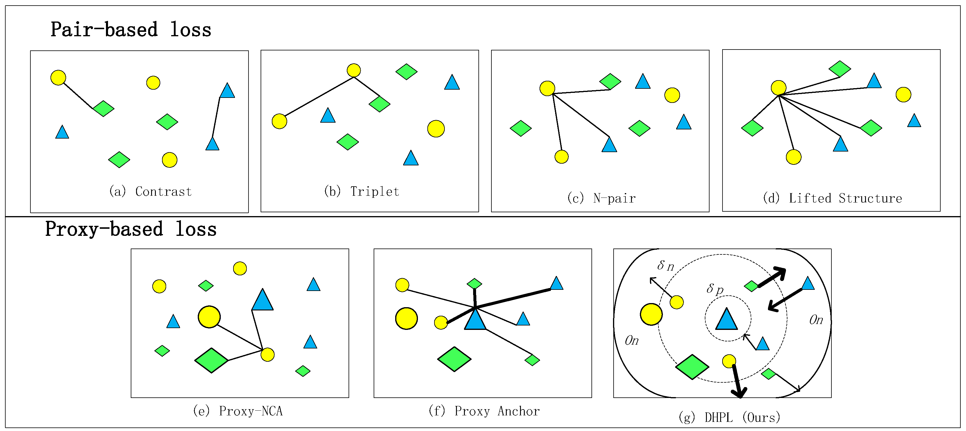
Proxy-based metric learning [21,22,23,24] is an approach used in recent years. It can solve the training time complexity problem of the pair-to-pair methods. A proxy is initialized with the network parameters and optimized as the network parameters are optimized. It can represent part of the samples. The common idea of such methods is to exploit a group of proxies that maintain the global structure of the embedded feature space and associate each data point to the proxy, rather than another sample during training. Since the quantity of proxies is greatly reduced relative to the number of training samples, time consumption can be greatly reduced. Proxy-NCA [21] is the first proxy-based loss. Proxy-NCA loss assigned one proxy to each category, and the number of proxies is the same as the number of category labels. It then associates each data point with all the proxies. Finally, it can make similar samples close together and dissimilar samples far apart. SoftTriple loss [23] assigns more than one proxy to each category to maintain greater intra-class distribution. Although these methods are able to greatly reduce the slow convergence, they are still very restrictive in maintaining the relationship between data-to-data relations. Proxy anchor loss [24] aims to overcome Proxy-NCA’s limitation, namely that it fails to maintain information between the pairs of samples. Proxy anchor loss uses proxies as anchors, and uses all the samples to associate with an anchor to consider the relationship between samples during training. It combines the benefits of proxy-based loss and pair-based loss. We constructed our tuples based on this. However, it still has the problem of fuzzy convergence states. We define the convergence state clearly and derive our loss from it. Our proposed DHPL defines explicit convergence states and constantly adjusts the training direction and intensity through the current state. Figure 1 shows the tuple structure of the different methods.
The hashing method is widely used in large data retrieval because of its small space requirements and fast retrieval speed. The goal of the hashing method is to train several nonlinear functions to encode high-dimensional float features to low-dimensional binarization features. Ordinarily, there are two hashing methods: unsupervised hashing methods and supervised hashing methods. Unsupervised hashing methods train networks with samples without label information. For example, spectral hashing (SH) [40] is an unsupervised hashing method. It utilizes recent results on the convergence of graph Laplacian eigenvectors to the Laplace-Beltrami eigenfunctions of the manifolds. Iterative quantization (ITQ) [26] is first applied to the original spatial datasets using PCA dimension reduction processing, then the problem can be converted into a dataset of data points mapped to binary super cube vertices, making corresponding quantitative error minimal, resulting in an excellent binary code for the data set.
Supervised hashing methods using label information can thus obtain higher retrieval accuracy. The kernel-based supervised hashing (KSH) method [25] utilizes Hamming distance and the coding of inner product equivalence, allowing a very efficient and easily optimized objective function to be obtained. Density sensitive hashing (DSH) [41] explores the geometric information of the samples and uses projection functions that best fit the data distribution. Nevertheless, the manual features used by traditional hashing methods are not flexible enough for the learning of hash features. Due to the learning ability of deep neural networks, more hash methods researchers have begun to use deep hash methods.
The deep hashing method can make full use of the learning characteristics of deep neural networks, which can improve retrieval accuracy and ensure retrieval speed. For instance, a deep hashing neural network (DHNN) [37] uses neural networks to learn high-dimensional embedding features and deep hashing learning networks to learn low-dimensional features. It can be optimized end-to-end. Deep hashing convolutional neural networks (DHCNN) [39] use the deep hashing method to perform retrieval and classification operations simultaneously, and achieve good hashing retrieval effects. In this paper, we introduce a new hashing method, which implements the efficient learning of features using a proxy-based loss.
3. Our Deep Hashing Using Proxy Loss Approach
In Section 3, we introduce four parts altogether. Section 3.1 elaborates on the metric learning loss function. Section 3.2 explicates quantization loss function. The architecture of the total network is showed in Section 3.3.
3.1. Proxy-Based Loss
Currently, pair-based loss has achieved excellent retrieval results by digging into the relationship between samples in depth. However, this method also has a great time complexity, due to the traversal collection of sample teams. Proxy-based losses can solve this problem. Proxies are generated as sample representatives, which greatly reduce the time cost of sample team collection. Moreover, the proxy-based method [21,22,23,24] has achieved good retrieval results. The biggest disadvantage of the proxy-based loss is that it cannot explore the information between samples well. Based on the above ideas, we present a method to explore the information between samples, and while using proxies to reduce the training time and maintain the global structure. At the same time, considering that most of the current losses cannot define the final optimization state, we also define the final optimization state of our losses in order to achieve effective training. First, we give the form of the loss function:
represents the set of positive proxies of the data, and P represents all proxies in the batch. For each proxy, the sample set similar to it is represented as , and the sample set different from it is represented as . is used to adjust the optimization direction of the positive sample, which can make the positive sample optimize in the direction, and towards the degree of, the optimal solution. is used to adjust the optimization direction and the degree of the negative sample, which can make the negative sample optimize in the direction of the optimal solution. is the threshold value that constrains the positive sample pair, which can ensure that the similarity between the positive sample pairs is greater than the specified value. is the margin used to make the similarity of all negative pairs smaller than it. In general, similarity can be measured using either Euclidean distance or cosine distance. They use distance and angle, respectively, to measure similarity. In our experiment, cosine similarity is used to measure distance in the training stage, and Hamming distance is used in the test stage. denotes the cosine similarity between hash codes and proxies defined in the corresponding category, and denotes the cosine similarity between hash codes and proxies defined in different categories. We give the formula for calculating the cosine similarity,
where K represents hash code length, represents the i-th dimension of hash code , and represents the i-th dimension of proxy . However, the measurement learning loss function is mainly used to learn representative features, while the hash code will lose some information. Moreover, discrete values make it difficult to calculate derivatives. Therefore, we use the hash-like features before quantization to calculate the similarity.
where K represents hash-like code length, and it is the same as the hash code. represents the i-th dimension of hash-like feature .
Multi-similarity loss [17] makes a detailed analysis of the weights of positive and negative sample pairs. It proposes self-similarity and two relative similarities, and the analysis of existing losses. Then construct their losses by all three similarities. We also analyze our losses in terms of the weights and give meaningful parameter values. If the similarity between two samples of the same kind is 1, then this is the best result between the positive sample pairs. Similarly, if the similarity between two samples of different categories is −1, then this is also the best result between the two negative sample pairs. These are two cases where no further optimization is required. The optimization purpose of our network is to bring the similarity between positive samples close to 1. Hence, we set to 1 − m in the expectation that it will clarify the final result of the network optimization. Network optimization refers to gradually optimizing network parameters through gradient calculation and back propagation during training, so that the trained network is more suitable for the current data situation. The optimization purpose of our network is also to bring the similarity between negative samples close to −1. Hence, we set to −1 + m in the expectation that it will clarify the final result of the network optimization. Be aware that m is a positive number greater than 0.
Usually, and can determine the way and speed of our optimization. Ideally, for samples that have been correctly classified as having the optimal similarity, we would prefer not to optimize them. For samples of correct classification close to optimal similarity, we would like to perform a weak optimization operation. For misclassified samples far from the optimal similarity, we would like to strongly optimize them. Based on the above analysis, we give the formula for the and .
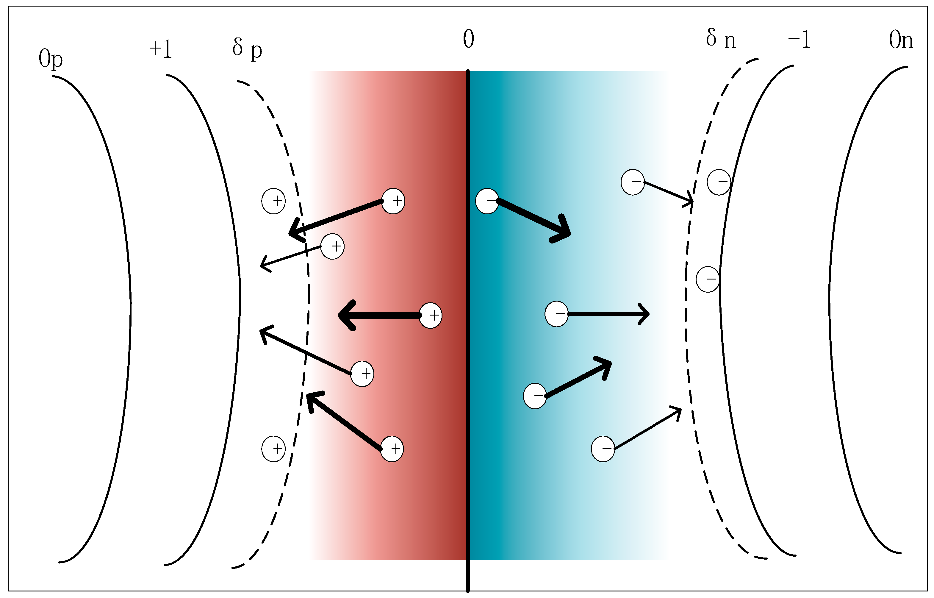
where is the result with the best similarity we expect between the positive sample pairs, and we set it to be a little bit bigger than 1 as 1 + m. is the result we expect with the optimal similarity value of the negative sample pairs, and we set it a little smaller than −1 as −1 − m. We use Figure 2 to represent the optimization of the sample.
3.2. Hashing Method
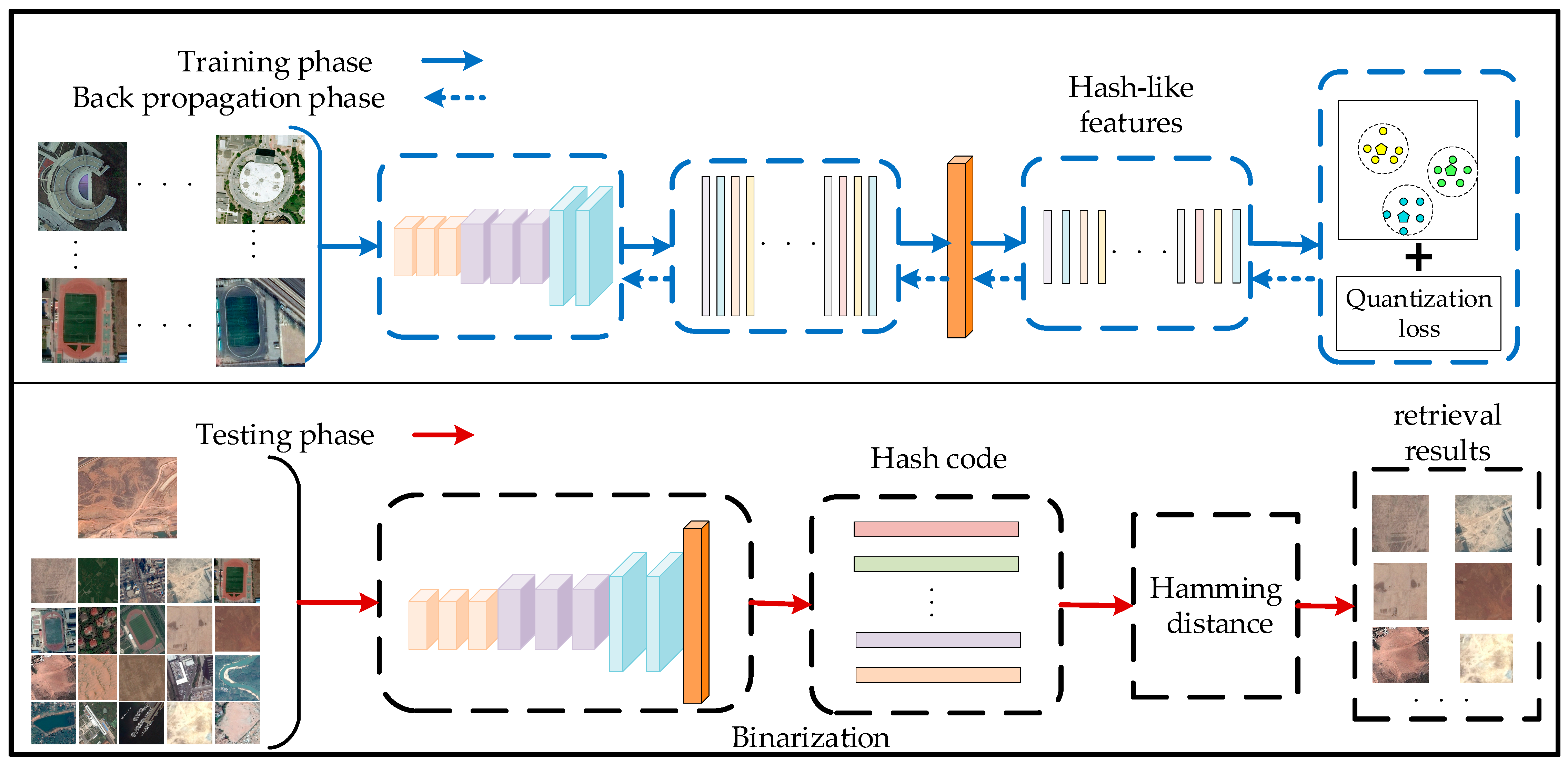
In order to reduce the high-dimensional features, we adopt the deep hash method to automatically learn the hash code. Specifically, we use a full connection layer for dimension reduction operations while being able to effectively learn the network parameters. We use Figure 3 to specifically show the architecture of our hashing method.
We first utilize deep CNN to obtain deep embedding features. Then, a full-connection layer is connected to shorten the length of the deep embedding features, and we get low-dimensional features. The dimension reduction function is:
denotes the parameters of the full connection layer. is the deep embedding features before dimensionality reduction. b is the bias. are the hash-like features. K are the dimensions of the hash code. For convenience, we call the low-dimensional features before quantization hash-like features. We use to obtain the hash code which we need to binarize the hash-like features. is a step function, and it returns a variant (integer) indicating the positive or negative sign of the parameter. For positive numbers, we get 1, and for negative numbers we get −1.
Intuitively, the binarization process causes an information loss, so a quantitative loss is necessary.
where is the i-th deep embedding feature of K bits, and is the i-th hash code of K bits. N is the batch size. denotes an -norm vector used to reduce the distance between hash code and hash-like code.
3.3. Time Complexity Analysis
In order to study the efficiency of deep hashing proxy loss, this section analyzes and compares the training complexity of different loss functions and the time consumption in the test retrieval stage. Assume that Q, M, and N represent the number of data samples in a batch, the number of sample categories, and the number of proxies of each class, respectively. In general, the magnitude of M is much less than Q. The comparison situations are listed in Table 1.
With the exception of SoftTriple loss, which allocates multiple proxies for each category, all the other types of proxy-based losses assign one proxy for each category, i.e., N = 1. For pair-based loss functions, contrastive loss takes sample pairs as input, and its time complexity is . Triplet loss takes triples into account, and its time complexity is , the same as N-pair loss and lifted structure loss. Of course, if a certain sampling technology is adopted to screen the data of the input network, the time complexity will be reduced to a certain extent. The training time consumption of the proxy-based loss is generally less than that of the pair-to-pair loss. Proxy-NCA loss and proxy-NCA++ loss in each data sample are related to a positive proxy and (M − 1) negative proxies, and therefore the training complexity is . In the SoftTriple loss, each class is represented by multiple proxies, and each data sample includes N positively correlated proxies and negatively correlated proxies, and the total training complexity is . The DHPL method mentioned in this chapter allocates a proxy for each category, and dynamically optimizes its training according to the similarity between the proxy and the data, and the similarity between the optimal value. The computational complexity of its training is , the same as that of the proxy-NCA.
As for the complexity of the test phase, we focus on the retrieval phase. In the retrieval stage, since we use the low latitude features of binary codes, compared with the high latitude features of floating-point values, we can greatly reduce the space requirements of retrieval features. At the same time, the calculation time cost of Hamming distance is much less than that of Euclidean distance and cosine distance.
Retrieval time is reduced, mainly because the calculation time of the Hamming distance is far less than that of the calculation time of the floating-point characteristic distance, while the very short hash code length can also reduce the retrieval time consumption.
The reduction in the physical storage space is, on the one hand, due to the length of the hash code, which is very short. On the other hand, binary code can also greatly reduce the space required compared to floating-point eigenvalues, and when the amount of data is increased, this saves considerable physical.
Reduction in retrieval time and reduced storage space are the root reasons for the application of the hash method.
4. Experiments
Section 4 introduces four parts. Section 4.1 first explains two popular RS datasets, and we show our formula for evaluation criteria. Section 4.2 lists the steps of our experimental implementation, and Section 4.3 shows the results of our experiment, and we analyze the results with a state-of-art method. In Section 4.4, we discuss our findings.
4.1. Dataset and Protocols
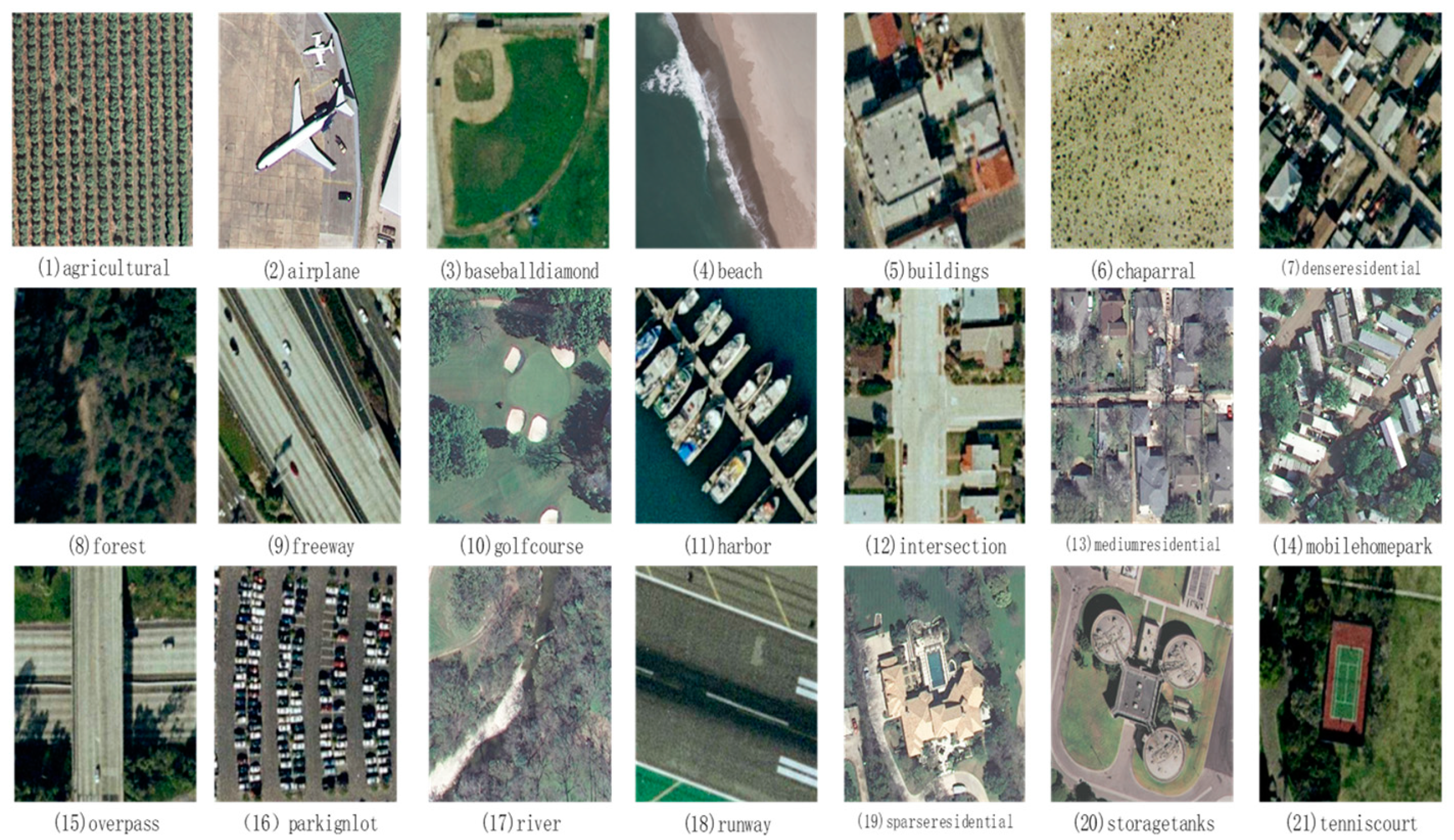
We mainly use two kinds of remote sensing images as the experimental data set: they are the UCMD and the AID. The UCMD [42] (University of California Merced, CA, USA dataset) is a public free remote sensing data set. The UCMD has 21 different categories of surface images, each of which contains 100 images, some of which include a large number of surface structures. The pixel size of the images is 256 × 256, and the spatial resolution is 0.3 m. Figure 4 shows pictures from the UCMD.
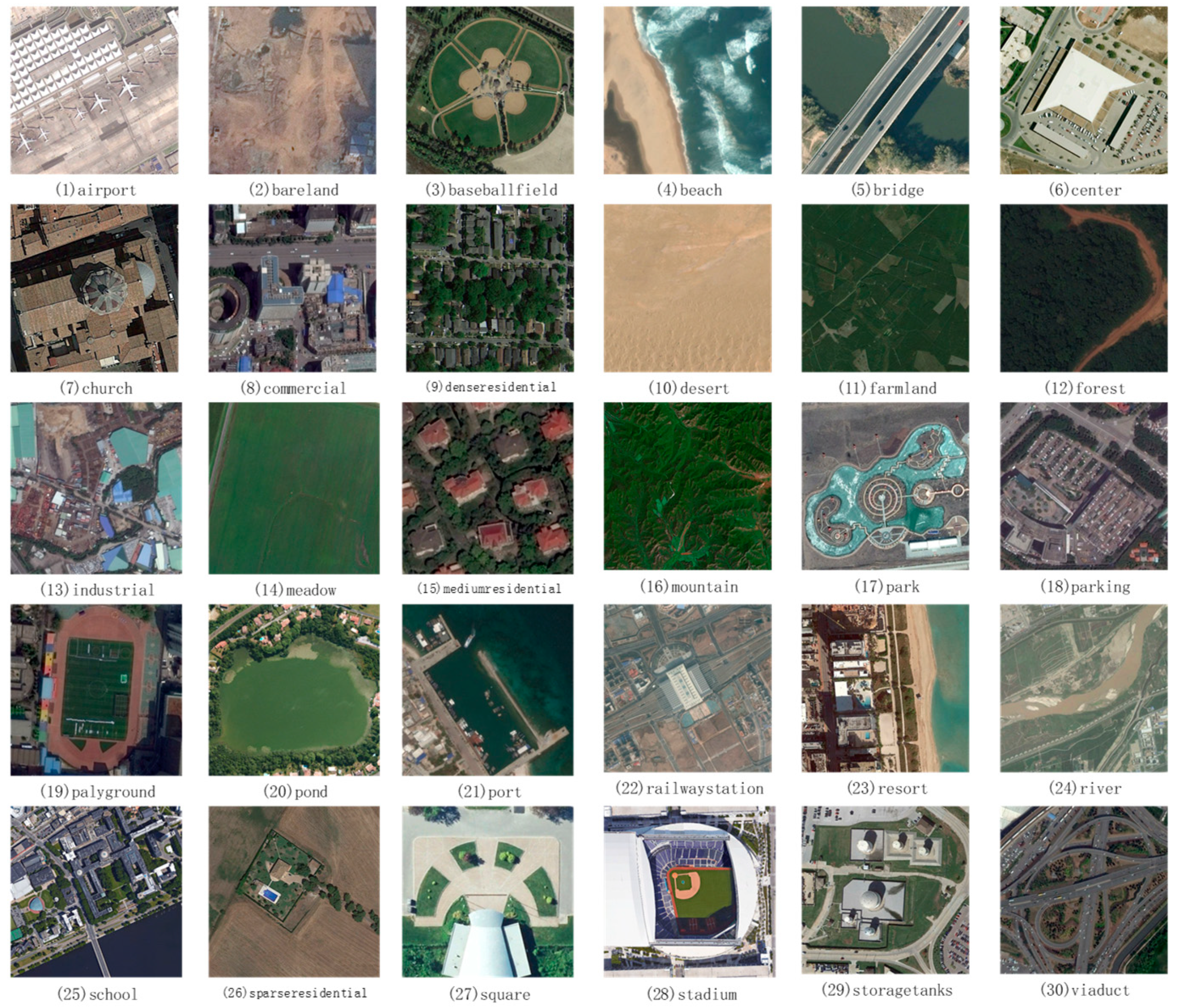
The AID [43] (Aerial Image Dataset) was obtained from Google Earth, and the pixel size of each image is equal to 600 × 600. The AID has 10,000 images in 30 categories. For both of these two data sets, images from the same category are treated as the ground-truth neighbors. Figure 5 shows pictures from the AID.
To compare the effects of different retrieval methods, we need to use the evaluation criteria common to other retrieval methods. We used mAP (mean average precision) as the evaluation criteria, which is consistent with that used in the DHCNN [39] method. Specifically, the value of mAP can be calculated by
where is the retrieval data set obtained from the i-th test sample, including a total of images. is the j-th image in dataset. || is the number of the testing set.
4.2. Implementation Details
We use a VGG-F network [44] pre-trained on ImageNet [45] as our basic network. Then the network parameters were fine-tuned using the remote sensing data set and the loss function we designed, in the hope that it can adapt more to the hash retrieval requirements of our remote sensing images. We set the output length of the last layer according to the length of the hash code, and L2-normalized the final output.
We used the AdamW optimizer [46] in each experiment, which has the same update step as Adam [47], but can attenuate weights separately. Our DHPL network is trained using an initial learning rate of 0.0001 on the UCMD and the AID datasets. To accelerate the proxy convergence, its learning rate is equal to 0.01. Input training batches are randomly selected during training.
Our training batch size was set to 90. We divided our training and test sets by 8:2 for the UCMD dataset, and by 5:5 for the AID dataset. One proxy was assigned for each class, and we initialized proxies using normal distributions to make sure that they were evenly distributed over the unit hyper sphere. The value of the m was set to 0.25.
4.3. Experimental Results
In this part, we give the experimental results on the UCMD and the AID, respectively, and analyze the obtained results so as to explain the effect of the DHPL method.
4.3.1. Results on UCMD
First, we compare the methods on a remote sensing data set, the UCMD. It consists of 20 species of remote sensing landmarks and 2000 images. According to the most common practice, we divided the data set such that the first 80 images in one class were utilized for training and the rest of the 20 images for testing. In order to estimate the effectiveness of our DHPL method, we listed some state-of-the-art methods, including DHCNN [39], DHNN-L2 [37], DPSH [4], KSH [31], ITQ [26], SELVE [30], DSH [41], and SH [25].
Table 2 shows the mAP results of the above methods and our method, with Hamming distance. Our experiment gives the results of four different hash code bits, varying from 16 bits to 64 bits. Notably, for the traditional methods KSH, ITQ, SELVE, DSH, and SH, we present results using CNN and using GIST features, respectively, which they represent using -CNN and -GIST.
The data in Table 2 shows that DHPL has the best results on all four hash bits on the UCMD dataset. When the length of the hash codes are 16 bits, our result is 2.01 (from 96.52 to 98.53) higher than the DHCNN method. When the hash code is 32 bits, our result is 1.85 (from 96.98 to 98.83) higher than the DHCNN method. When the hash code is 48 bits, our result is 1.55 (from 97.46 to 99.01) higher than the DHCNN method. When the hash code is 64 bits, our result is 1.19 (from 98.02 to 99.21) higher than the DHCNN method. Compared with other methods, we have a significant improvement in retrieval accuracy. We can also see that for traditional methods, the CNN methods can achieve better results than the GIST methods, which shows that the network can achieve a better learning effect because of its self-optimization ability. From the results, we find that when the hash code is shorter, the results obtained by our network are slightly worse. The reason is fore this is that a significant information loss occurs when the hash code length continues to decrease to a certain dimension.
4.3.2. Results on AID
We conduct the experiments on the AID data set, which contains 30 kinds of aerial photography landscapes and 10,000 images. We use the first 50% of images in one class for training, and the remaining images for testing. We also compared different kinds of state-of-the-art hashing methods, including DHCNN [39], DHNN-L2 [37], DPSH [4], KSH [30], ITQ [26], SELVE [30], DSH [41], and SH [25]. Table 3 shows the mAP results of 14 kinds of hashing methods with Hamming distance. Our experiment gives the results of four kind of hash code, with bits varying from 16 bits to 64 bits.
The data in Table 3 illustrates that our DHPL method has the best results on all four hash bits on the UCMD dataset. When the length of the hash code is 16 bits, our result is 4.48 (from 89.05 to 93.53) higher than the DHCNN method. When the hash code is 32 bits, our result is 4.39 (from 92.97 to 97.36) higher than the DHCNN method. When the hash code is 48 bits, our result is 4.07 (from 94.21 to 98.28) higher than the DHCNN method. When hash code is 64 bits, our result is 4.27 (from 94.27 to 98.54) higher than the DHCNN method. Compared with other methods, we have a significant retrieval effect. We can also see that, for traditional methods, the CNN methods can achieve better results than the GIST methods. On the AID datasets, the 16-bit hash codes also lose much more retrieval accuracy than the high-dimensional hash codes.
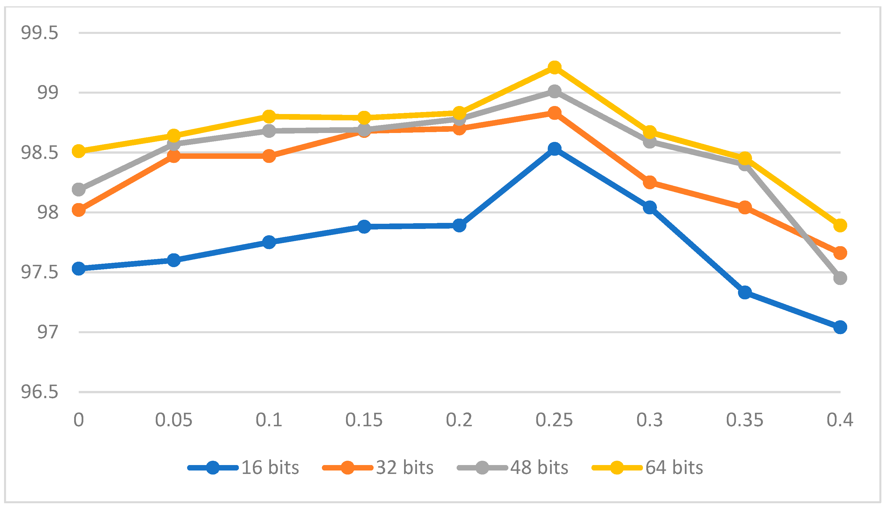
In order to show the retrieval effect under different hyper-parameter m, we enumerate the results of ablation experiments on the remote sensing dataset UCMD. We list the results of different hash bits. The experimental results are given in the form of a line chart. We adjusted the m value gradually. It was varied from 0.5 to 1.0. Figure 6 shows the result.
As can be seen from Figure 6, the greater the length of the hash code, the greater the retrieval accuracy. At the same time, when the value of m changes from small to large, the accuracy also changes. Therefore, we set the m value to 0.25, where the accuracy is maximized.
4.4. Disscussion
In light of the above experimental results, we discovered that our DHPL method has the best results on the UCMD and AID datasets. Our DHPL not only has the superior retrieval speed of the hash method, but also has the advantage of the fast training speed of the proxy-based method. Furthermore, longer hash bits all receive better retrieval results because they save more information, while shorter hash bits all receive worse retrieval results because they lose a lot of information due to dimension reduction. However, we expect to use the hash method to reduce the memory space and retrieval time. Through the above experiments, we also find that there are hash lengths with both moderate length and well-preserved accuracy, allowing the most appropriate hash lengths in specific scenarios to be selected according to the experiment. In remote sensing image scenarios, 32 bits can be selected as the length of the hash code to ensure specific performance costs. As for the selection of network, we chose it based on our experience from previous work, and the initial parameters of the network were obtained through pre-training. Finally, it is worth mentioning that our DHPL can acquire excellent results with proxy-based metric learning loss and binarization loss.
5. Conclusions
In this paper, we use one proxy-based hash retrieval method, called Deep Hashing using Proxy Loss (DHPL), which combines hash code learning with proxy-based metric learning in a convolutional neural network. Specifically, we designed a novel proxy metric learning loss which can learn the network by constantly adjusting the relationship between the current state and the optimal state. We used one hash loss formula to reduce the quantified losses. Our experimental results on two widely used datasets demonstrate that DHPL could generate better results than other state-of-the-art hashing methods.
This work focused on remote sensing data sets, and we did not make many changes in the network structure. Next, we will apply hashing in more directions and make improvements in the network structure.
Author Contributions
P.L. determined the research direction, gave innovative ideas, modified the article expression, and knew the work process. X.S. conducted the experiment and completed the first paper. Y.W., Z.W., and Q.Z. checked out the article’s writing. All authors have read and agreed to the published version of the manuscript.
Funding
This research was supported by the Nature Science Foundation of China, under Grants 61841602, 62071199 the fundamental Research Funds of Central Universities, JLU, General Financial Grant from China Postdoctoral Science Foundation, under Grants 2015M571363 and 2015M570272, the Provincial Science and Technology Innovation Special Fund Project of Jilin Province, under Grant 20190302026GX, the Jilin Province Development and Reform Commission Industrial Technology Research and Development Project, under Grant 2019C054-4, the Graduate Innovation Fund of Jilin University and the State Key Laboratory of Applied Optics Open Fund Project, under Grant20173660. Jilin Provincial Natural Science Foundation No.20200201283JC. Foundation of Jilin Educational Committee No. JJKH20200994K.
Acknowledgments
Thanks to the School of Computer Science and Technology of Jilin University for its support of the experimental equipment.
Conflicts of Interest
The authors declare no conflict of interest.
References
- Ma, Y.; Wu, H.; Wang, L.; Huang, B.; Ranjan, R.; Zomaya, A.; Jie, W. Remote sensing big data computing: Challenges and opportunities. Futur. Gener. Comput. Syst. 2015, 51, 47–60. [Google Scholar] [CrossRef] [Green Version]
- Schroff, F.; Kalenichenko, D.; Philbin, J. FaceNet: A unified embedding for face recognition and clustering. In Proceedings of the IEEE Conference on Computer Vision and Pattern Recognition, Boston, MA, USA, 7–12 June 2015; pp. 815–823. [Google Scholar]
- Szegedy, C.; Vanhoucke, V.; Ioffe, S.; Shlens, J.; Wojna, Z. Rethinking the Inception Architecture for Computer Vision. In Proceedings of the 2016 IEEE Conference on Computer Vision and Pattern Recognition (CVPR), Las Vegas, NV, USA, 27–30 June 2016; pp. 2818–2826. [Google Scholar] [CrossRef] [Green Version]
- Li, W.; Wang, S.; Kang, W.-C.J.A. Feature Learning Based Deep Supervised Hashing with Pairwise Labels. arXiv 2016, arXiv:1511.03855. [Google Scholar]
- Sumbul, G.; Kang, J.; Demir, B.J.A. Deep Learning for Image Search and Retrieval in Large Remote Sensing Archives. arXiv 2020, arXiv:2004.01613. [Google Scholar]
- Dai, O.E.; Demir, B.; Sankur, B.; Bruzzone, L. A Novel System for Content-Based Retrieval of Single and Multi-Label High-Dimensional Remote Sensing Images. IEEE J. Sel. Top. Appl. Earth Obs. Remote Sens. 2018, 11, 2473–2490. [Google Scholar] [CrossRef] [Green Version]
- Tong, X.-Y.; Xia, G.-S.; Hu, F.; Zhong, Y.; Datcu, M.; Zhang, L. Exploiting Deep Features for Remote Sensing Image Retrieval: A Systematic Investigation. IEEE Trans. Big Data 2020, 6, 507–521. [Google Scholar] [CrossRef] [Green Version]
- Zhao, L.; Tang, J.; Yu, X.; Li, Y.; Mi, S.; Zhang, C. Content-Based Remote Sensing Image Retrieval Using Image Multi-feature Combination and SVM-Based Relevance Feedback. In Recent Advances in Computer Science and Information Engineering; Springer: Berlin/Heidelberg, Germany, 2012; Volume 124, pp. 761–767. [Google Scholar]
- Daschiel, H.; Datcu, M. Information mining in remote sensing image archives: System evaluation. IEEE Trans. Geosci. Remote Sens. 2005, 43, 188–199. [Google Scholar] [CrossRef]
- Lowe, D.G. Similarity Metric Learning for a Variable-Kernel Classifier. Neural Comput. 1995, 7, 72–85. [Google Scholar] [CrossRef]
- Xing, E.P.; Ng, A.Y.; Jordan, M.I.; Russell, S.J. Distance Metric Learning with Application to Clustering with Side-Information. In Proceedings of the International Conference on Neural Information Processing Systems, Vancouver, BC, Canada, 9–14 December 2002. [Google Scholar]
- Hadsell, R.; Chopra, S.; LeCun, Y. Dimensionality Reduction by Learning an Invariant Mapping. In Proceedings of the 2006 IEEE Computer Society Conference on Computer Vision and Pattern Recognition-Volume 2 (CVPR’06), New York, NY, USA, 17–22 June 2006; Volume 2, pp. 1735–1742. [Google Scholar]
- Hoffer, E.; Ailon, N. Deep Metric Learning Using Triplet Network. In Proceedings of the International Workshop on Similarity-Based Pattern Recognition. SIMBAD 2015. Lecture Notes in Computer Science, Copenhagen, Denmark, 12–14 October 2015; Springer: Cham, Switzerland, 2015; Volume 9370. [Google Scholar] [CrossRef] [Green Version]
- Song, H.O.; Xiang, Y.; Jegelka, S.; Savarese, S. Deep Metric Learning via Lifted Structured Feature Embedding. In Proceedings of the 2016 IEEE Conference on Computer Vision and Pattern Recognition (CVPR), Las Vegas, NV, USA, 27–30 June 2016. [Google Scholar]
- Sohn, K. Improved deep metric learning with multi-class N-pair loss objective. In Proceedings of the 29th International Conference on Neural Information Processing Systems, Barcelona, Spain, 5–10 December 2016. [Google Scholar]
- Sun, Y.; Cheng, C.; Zhang, Y.; Zhang, C.; Zheng, L.; Wang, Z.; Wei, Y.J.I. Circle Loss: A Unified Perspective of Pair Sim-ilarity Optimization. In Proceedings of the IEEE/CVF Conference on Computer Vision and Pattern Recognition, Seattle, WA, USA, 14–19 June 2020. [Google Scholar]
- Wang, X.; Han, X.; Huang, W.; Dong, D.; Scott, M.R. Multi-Similarity Loss with General Pair Weighting for Deep Metric Learning. In Proceedings of the 2019 IEEE/CVF Conference on Computer Vision and Pattern Recognition (CVPR), Long Beach, CA, USA, 15–20 June 2019. [Google Scholar]
- Harwood, B.; Vijay Kumar, B.G.; Carneiro, G.; Reid, I.; Drummond, T. Smart Mining for Deep Metric Learning. In Proceedings of the 2017 IEEE International Conference on Computer Vision (ICCV), Venice, Italy, 22–29 October 2017. [Google Scholar]
- Wu, C.-Y.; Manmatha, R.; Smola, A.J.; Krahenbuhl, P. Sampling Matters in Deep Embedding Learning. In Proceedings of the 2017 IEEE International Conference on Computer Vision (ICCV), Venice, Italy, 22–29 October 2017. [Google Scholar]
- Yuan, Y.; Yang, K.; Zhang, C. Hard-Aware Deeply Cascaded Embedding. In Proceedings of the 2017 IEEE International Conference on Computer Vision (ICCV), Venice, Italy, 22–29 October 2017. [Google Scholar]
- Movshovitz-Attias, Y.; Toshev, A.; Leung, T.K.; Ioffe, S.; Singh, S. No Fuss Distance Metric Learning Using Proxies. In Proceedings of the 2017 IEEE International Conference on Computer Vision (ICCV), Venice, Italy, 22–29 October 2017. [Google Scholar]
- Teh, E.W.; Devries, T.; Taylor, G.W.J.S. ProxyNCA++: Revisiting and Revitalizing Proxy Neighborhood Compo-nent Analysis. In Computer Vision–ECCV 2020, Proceedings of the 16th European Conference, Glasgow, UK, 23–28 August 2020; Springer International Publishing: Berlin/Heidelberg, Germany, 2020. [Google Scholar]
- Qian, Q.; Shang, L.; Sun, B.; Hu, J.; Tacoma, T.; Li, H.; Jin, R. SoftTriple Loss: Deep Metric Learning Without Triplet Sampling. In Proceedings of the 2019 IEEE/CVF International Conference on Computer Vision (ICCV), Seoul, Korea, 27 October–3 November 2019. [Google Scholar]
- Kim, S.; Kim, D.; Cho, M.; Kwak, S. Proxy Anchor Loss for Deep Metric Learning. In Proceedings of the 2020 IEEE/CVF Conference on Computer Vision and Pattern Recognition (CVPR), Seattle, WA, USA, 16–18 June 2020. [Google Scholar]
- Weiss, Y.; Torralba, A.; Fergus, R. Spectral Hashing. In Proceedings of the International Conference on Neural Information Processing Systems, Whistler, BC, Canada, 11 December 2009; Volume 282, pp. 1753–1760. [Google Scholar]
- Gong, Y.; Lazebnik, S.; Gordo, A.; Perronnin, F. Iterative Quantization: A Procrustean Approach to Learning Binary Codes for Large-Scale Image Retrieval. IEEE Trans. Pattern Anal. Mach. Intell. 2013, 35, 2916–2929. [Google Scholar] [CrossRef] [PubMed] [Green Version]
- Liu, W.; Mu, C.; Kumar, S.; Chang, S.F. Discrete Graph Hashing. In Proceedings of the Advances in Neural Information Processing Systems, Montreal, QC, Canada, 13 December 2014; Volume 4, pp. 3419–3427. [Google Scholar]
- Kulis, B.; Darrell, T. Learning to Hash with Binary Reconstructive Embeddings. In Proceedings of the International Conference on Neural Information Processing Systems, Vancouver, BC, Canada, 8–14 December 2009. [Google Scholar]
- Norouzi, M.E.; Fleet, D.J. Minimal Loss Hashing for Compact Binary Codes. In Proceedings of the 28th International Conference on Machine Learning, ICML 2011, Bellevue, WA, USA, 28 June–2 July 2011. [Google Scholar]
- Zhu, X.; Zhang, L.; Huang, Z. A Sparse Embedding and Least Variance Encoding Approach to Hashing. IEEE Trans. Image Process. 2014, 23, 3737–3750. [Google Scholar] [CrossRef] [PubMed] [Green Version]
- Liu, W.; Wang, J.; Ji, R.; Jiang, Y.-G.; Chang, S.-F. Supervised hashing with kernels. In Proceedings of the 2012 IEEE Conference on Computer Vision and Pattern Recognition, Washington, DC, USA, 16–21 June 2012. [Google Scholar]
- Lowe, D.G. Distinctive Image Features from Scale-Invariant Keypoints. Int. J. Comput. Vision 2004, 60, 91–110. [Google Scholar] [CrossRef]
- Oliva, A.; Torralba, A. Modeling the Shape of the Scene: A Holistic Representation of the Spatial Envelope. Int. J. Comput. Vis. 2001, 42, 145–175. [Google Scholar] [CrossRef]
- Babenko, A.; Slesarev, A.; Chigorin, A.; Lempitsky, V. Neural Codes for Image Retrieval. In Proceedings of the European Conference on Computer Vision, Zurich, Switzerland, 6–12 September 2014. [Google Scholar]
- Krizhevsky, A.; Hinton, G.E. Using Very Deep Autoencoders for Content-Based Image Retrieval. In Proceedings of the European Symposium on Esann, Bruges, Belgium, 27–29 April 2011. [Google Scholar]
- Xu, Z.; Mahalingam, M.; Tang, C. Semantic Hashing. U.S. Patent 20040088274, 6 5 2004. [Google Scholar]
- Li, Y.; Zhang, Y.; Huang, X.; Zhu, H.; Ma, J. Large-Scale Remote Sensing Image Retrieval by Deep Hashing Neural Networks. IEEE Trans. Geosci. Remote Sens. 2017, 56, 950–965. [Google Scholar] [CrossRef]
- Li, Y.; Zhang, Y.; Huang, X. Learning Source-Invariant Deep Hashing Convolutional Neural Networks for Cross-Source Remote Sensing Image Retrieval. IEEE Trans. Geosci. Remote Sens. 2018, 56, 6521–6536. [Google Scholar] [CrossRef]
- Song, W.; Li, S.; Benediktsson, J.A.; Sensing, R. Deep Hashing Learning for Visual and Semantic Retrieval of Remote Sensing Images. IEEE Trans. Geosci. Remote Sens. 2020. [Google Scholar] [CrossRef]
- Gold Be Rger, J.; Roweis, S.T.; Hinton, G.E.; Salakhutdinov, R. Neighbourhood Components Analysis. In Proceedings of the Advances in Neural Information Processing Systems, Vancouver, BC, Canada, 13–18 December 2004. [Google Scholar]
- Jin, Z.; Li, C.; Lin, Y.; Cai, D. Density Sensitive Hashing. IEEE Trans. Cybern. 2013, 44, 1362–1371. [Google Scholar] [CrossRef] [PubMed] [Green Version]
- Bag-of-visual-words and spatial extensions for land-use classification. In Proceedings of the 18th ACM SIGSPATIAL International Symposium on Advances in Geographic Information Systems, ACM-GIS 2010, San Jose, CA, USA, 3–5 November 2010.
- Xia, G.-S.; Hu, J.; Hu, F.; Shi, B.; Bai, X.; Zhong, Y.; Zhang, L.; Lu, X. AID: A Benchmark Data Set for Performance Evaluation of Aerial Scene Classification. IEEE Trans. Geosci. Remote Sens. 2017, 55, 3965–3981. [Google Scholar] [CrossRef] [Green Version]
- Ioffe, S.; Szegedy, C. Batch normalization: Accelerating deep network training by reducing internal covariate shift. In Proceedings of the International conference on machine learning, Lille, France, 6–11 July 2015. [Google Scholar]
- Deng, J.; Dong, W.; Socher, R.; Li, L.J.; Li, K.; Li, F.F. Imagenet: A Large-Scale Hierarchical Image Database. In Proceedings of the 2009 IEEE Conference on Computer Vision and Pattern Recognition, Miami, FL, USA, 20–25 June 2009; pp. 248–255. [Google Scholar]
- Loshchilov, I.; Hutter, F. Decoupled Weight Decay Regularization. arXiv 2017, arXiv:1711.05101. [Google Scholar]
- Kingma, D.P.; Ba, J. Adam: A method for stochastic optimization. arXiv 2014, arXiv:1414.6980. [Google Scholar]
Figure 1.
The structure diagram of the pair-based loss and the proxy-based loss is given in the figure. The graphs with different colors and shapes represent samples of different categories, among which the slightly smaller ones are actual sample points, and the slightly larger ones represent proxies of corresponding categories. Lines connecting different shapes represent pairs of samples that need to be constructed for training. The thicker lines represent greater optimization degree. The arrows point to the optimization direction, and the dotted circles represents the threshold ranges. The arc of the real lines represents the location of the optimal value , optimized for dissimilar samples. (a) Contrast loss [12] uses two samples to construct a sample pair. (b) Triplet loss [13] using a sample as the anchor, and a triplet is constructed by selecting both the same kind of positive sample and a different negative sample. (c) N-pair loss [15] and (d) lifted structure loss [14] construct tuples with more samples, but do not make use of all samples in the batch. (e) Proxy-NCA loss [21] associates each sample with proxies, but it does not explore the relationships between samples. (f) Proxy anchor loss [24] selects a proxy as an anchor and associates it with other samples. (g) Our DHPL loss is based on the proxy anchor and different optimization conditions are considered in DHPL loss.

Figure 2.
The dotted line represents the boundary of and , and the colored areas inside represent the areas that need to be optimized. The darker the color, the greater the optimization degree, and the lighter the color, the smaller the optimization degree. The circle with “+” is a positive sample, which is optimized toward the optimal direction, while the circle with “-” is a negative sample, which is optimized toward the optimal direction. At the same time, the direction of the arrow denotes the optimization direction, and the thickness indicates the optimization degree.

Figure 3.
Image retrieval framework based on deep hashing using Proxy Loss.

Figure 4.
Sample images of UCMD dataset.

Figure 5.
Sample images of AID dataset.

Figure 6.
mAP results of different hash bits under different m on UCMD dataset.


Table 1.
Comparison of training complexity of different loss functions.
| Loss Type | Loss | Training Complexity |
|---|---|---|
| Pair-based | Contrastive loss | |
| Triplet loss | ||
| N-pair loss | ||
| Lift Structure loss | ||
| Proxy-based | Proxy-NCA loss | |
| Proxy-NCA++ loss | ||
| SoftTriple Loss | ||
| Proxy-Anchor loss | ||
| DHPL(Ours) |
Table 2.
mAP retrieval results on the UCMD dataset, and we give separate hash retrieval results for 16, 32, 48, 64 bits. The testing set has 420 images (each category randomly takes 20% of the images). We have thickened the best results.
Table 2.
mAP retrieval results on the UCMD dataset, and we give separate hash retrieval results for 16, 32, 48, 64 bits. The testing set has 420 images (each category randomly takes 20% of the images). We have thickened the best results.
| Method | Hash Code Length | |||
|---|---|---|---|---|
| 16 bits | 32 bits | 48 bits | 64 bits | |
| DHPL (ours) | 98.53 | 98.83 | 99.01 | 99.21 |
| DHCNN [39] | 96.52 | 96.98 | 97.46 | 98.02 |
| DHNN-L2 [37] | 67.73 | 78.23 | 82.43 | 85.59 |
| DPSH [4] | 53.64 | 59.33 | 62.17 | 65.21 |
| KSH-CNN [30] | 75.50 | 83.62 | 86.55 | 87.22 |
| ITQ-CNN [26] | 42.65 | 45.63 | 47.21 | 47.64 |
| SELVE-CNN [30] | 36.12 | 40.36 | 40.38 | 38.58 |
| DSH-CNN [41] | 28.82 | 33.07 | 33.15 | 34.59 |
| SH-CNN [25] | 29.52 | 30.08 | 30.37 | 29.31 |
| KSH-GIST [30] | 38.75 | 43.27 | 44.44 | 46.38 |
| ITQ-GIST [26] | 19.85 | 20.44 | 20.67 | 20.96 |
| SELVE-GIST [30] | 17.24 | 18.18 | 18.08 | 18.17 |
| DSH-GIST [41] | 16.57 | 17.79 | 19.21 | 19.18 |
| SH-GIST [25] | 13.76 | 14.46 | 14.24 | 14.17 |
Table 3.
mAP retrieval results on the AID dataset, and we give separate hash retrieval results for 16, 32, 48, 64 bits. The test set has 5000 images (each category randomly takes 50% of the images). We have thickened the best results.
Table 3.
mAP retrieval results on the AID dataset, and we give separate hash retrieval results for 16, 32, 48, 64 bits. The test set has 5000 images (each category randomly takes 50% of the images). We have thickened the best results.
| Method | Hash Code Length | |||
|---|---|---|---|---|
| 16 bits | 32 bits | 48 bits | 64 bits | |
| DHPL(Ours) | 93.53 | 97.36 | 98.28 | 98.54 |
| DHCNN [39] | 89.05 | 92.97 | 94.21 | 94.27 |
| DHNN-L2 [37] | 57.87 | 70.36 | 73.98 | 77.20 |
| DPSH [4] | 28.92 | 35.30 | 37.84 | 40.78 |
| KSH-CNN [30] | 48.26 | 58.15 | 61.59 | 63.26 |
| ITQ-CNN [26] | 23.35 | 27.31 | 28.79 | 29.99 |
| SELVE-CNN [30] | 34.58 | 37.87 | 39.09 | 36.81 |
| DSH-CNN [41] | 16.05 | 18.08 | 19.36 | 19.72 |
| SH-CNN [25] | 12.69 | 16.99 | 16.16 | 16.21 |
| KSH-GIST [30] | 18.96 | 22.64 | 24.76 | 26.32 |
| ITQ-GIST [26] | 9.99 | 10.63 | 11.04 | 11.30 |
| SELVE-GIST [30] | 10.37 | 10.62 | 10.62 | 10.40 |
| DSH-GIST [41] | 9.35 | 9.35 | 9.74 | 10.05 |
| SH-GIST [25] | 6.71 | 7.02 | 6.97 | 6.95 |
Publisher’s Note: MDPI stays neutral with regard to jurisdictional claims in published maps and institutional affiliations. |
© 2021 by the authors. Licensee MDPI, Basel, Switzerland. This article is an open access article distributed under the terms and conditions of the Creative Commons Attribution (CC BY) license (https://creativecommons.org/licenses/by/4.0/).
Share and Cite
MDPI and ACS Style
Shan, X.; Liu, P.; Wang, Y.; Zhou, Q.; Wang, Z. Deep Hashing Using Proxy Loss on Remote Sensing Image Retrieval. Remote Sens. 2021, 13, 2924. https://0-doi-org.brum.beds.ac.uk/10.3390/rs13152924
AMA Style
Shan X, Liu P, Wang Y, Zhou Q, Wang Z. Deep Hashing Using Proxy Loss on Remote Sensing Image Retrieval. Remote Sensing. 2021; 13(15):2924. https://0-doi-org.brum.beds.ac.uk/10.3390/rs13152924
Chicago/Turabian StyleShan, Xue, Pingping Liu, Yifan Wang, Qiuzhan Zhou, and Zhen Wang. 2021. "Deep Hashing Using Proxy Loss on Remote Sensing Image Retrieval" Remote Sensing 13, no. 15: 2924. https://0-doi-org.brum.beds.ac.uk/10.3390/rs13152924
Note that from the first issue of 2016, this journal uses article numbers instead of page numbers. See further details here.