
Exploring the Use of PlanetScope Data for Particulate Matter Air Quality Research


1
The Earth System Science Center, The University of Alabama in Huntsville, Huntsville, AL 35899, USA
2
Department of Atmospheric and Earth Science, The University of Alabama in Huntsville, Huntsville, AL 35899, USA
3
Marshall Space Flight Center, Huntsville, AL 35808, USA
*
Author to whom correspondence should be addressed.
Remote Sens. 2021, 13(15), 2981; https://0-doi-org.brum.beds.ac.uk/10.3390/rs13152981
Submission received: 16 June 2021
/
Revised: 15 July 2021
/
Accepted: 23 July 2021
/
Published: 29 July 2021
Abstract
:Planet, a commercial company, has achieved a key milestone by launching a large fleet of small satellites (smallsats) that provide high spatial resolution imagery of the entire Earth’s surface on a daily basis with its PlanetScope sensors. Given the potential utility of these data, this study explores the use for fine particulate matter (PM2.5) air quality applications. However, before these data can be utilized for air quality applications, key features of the data, including geolocation accuracy, calibration quality, and consistency in spectral signatures, need to be addressed. In this study, selected Dove-Classic PlanetScope data is screened for geolocation consistency. The spectral response of the Dove-Classic PlanetScope data is then compared to Moderate Resolution Imaging Spectroradiometer (MODIS) data over different land cover types, and under varying PM2.5 and mid visible aerosol optical depth (AOD) conditions. The data selected for this study was found to fall within Planet’s reported geolocation accuracy of 10 m (between 3–4 pixels). In a comparison of top of atmosphere (TOA) reflectance over a sample of different land cover types, the difference in reflectance between PlanetScope and MODIS ranged from near-zero (0.0014) to 0.117, with a mean difference in reflectance of 0.046 ± 0.031 across all bands. The reflectance values from PlanetScope were higher than MODIS 78% of the time, although no significant relationship was found between surface PM2.5 or AOD and TOA reflectance for the cases that were studied. The results indicate that commercial satellite data have the potential to address Earth-environmental issues.
1. Introduction
A commercial company called Planet has launched a large fleet of small satellites (smallsats) called Doves, equipped with a sensor referred to as PlanetScope, that provide high-resolution (sub 5 m) imagery of the entire Earth’s surface on a daily basis. Surpassing the spatiotemporal coverage offered by most existing environmental satellites, this data has the potential to benefit a wide range of scientific applications at fine spatial scales. This paper first describes Planet’s platform in the context of other Earth observing satellites followed by a description of the current state of the data. This is important since the technology employed in Planet’s smallsat constellation is continuously evolving. Then, we consider the potential for using this data for air quality applications including fine particulate matter (PM2.5) estimation. Before this data can be utilized for air quality applications, key features of the data including geolocation accuracy, calibration quality, and consistency in spectral signatures need to be addressed. This paper presents the results of an initial exploratory study conducted to assess these attributes specifically for the Dove-Classic PlanetScope sensor.
1.1. PlanetScope in the Context of Earth Observing Satellite Remote Sensing
Smallsats, defined as satellites with a mass of 500 kg or less, have become increasingly popular for space-borne observation [1,2]. Smallsats gained traction in large part due to the success of the CubeSat standard, which launched in 1999 as a collaboration between California Polytechnic State and Stanford University [3,4]. Originally developed to make space more accessible to university students, the CubeSat standard provides a cost effective, off-the-shelf approach for space-borne observation and has since been adopted by organizations worldwide [4]. The standard CubeSat unit, 1U, measures 10 × 10 × 10 cm and can extend to larger sizes such as 1.5U, 2U, etc. Based on their size, CubeSats are considered either nanosatellites or picosatellites, in terms of commonly used smallsat categories [5].
Due to their accessibility, CubeSats and other smallsat designs have become competitive against larger traditional satellites. Traditional satellites are designed to carry highly specialized technologies that require years of research and development effort [2]. Traditional satellites also tend to be large, heavy, and therefore expensive to launch [2]. Smallsats, on the other hand, tend to employ commercially available off-the-shelf (COTS) technologies, and with recent advancements in the miniaturization of electronics, COTS have become smaller, lighter, cheaper, and more readily available [2]. As a result, smallsats are comparatively cheaper to develop and launch, although the availability of launch vehicles remains a hurdle [6]. These aspects also make smallsats resilient in the event of mission failure, since fewer resources are lost. It is also becoming more common to launch smallsats as part of a constellation of multiple coordinated satellites [1].
The accessibility of smallsat technology has helped open the industry to the private sector. While smallsats were once primarily developed by universities and research institutes, approximately 51% of smallsats are now produced by private companies [7,8]. One of these commercial smallsat companies is Planet (formerly Planet Labs), and its mission is to “image the entire Earth every day and make global change visible, accessible, and actionable” [9]. Planet’s mission is attractive since there is typically a trade-off between temporally frequent and high spatial resolution observations with data from traditional satellites. For instance, NASA’s Moderate Resolution Imaging Spectroradiometer (MODIS), flying on the twin Aqua and Terra polar orbiting sun synchronous satellites, can image the entire Earth’s surface every one to two days, but does so at a resolution of 250 to 1000 m [10]. At this resolution, finer-scale details needed for tracking regional and local trends are not resolvable. The Landsat mission, which is a joint venture between NASA and the USGS, provides data at a much finer 30 m spatial resolution. The revisit time for Landsat, however, is 16 days, leaving large gaps in the coverage needed for time-series analyses that require more frequent observations. This effect is exacerbated in cloudy locations where usable imagery may not be available for extended periods of time [11].
The more-recent European Space Agency (ESA) Sentinel-2 mission competes with Landsat capabilities by providing data at a 10–60 m resolution in comparable spectral bands, with a revisit time of 2–3 days at mid-latitudes and five days at the equator [12]. This is accomplished via a constellation of two identical satellites offset by 180 degrees in a polar orbit. ESA and NASA have also entered a collaborative agreement to cross-calibrate Sentinel-2 and Landsat’s multispectral sensors, paving the way for the Harmonized Landsat and Sentinel-2 surface reflectance (HLS) series of merged data products [13]. When completed, HLS will offer global surface reflectance data at a 30 m spatial resolution every 2–3 days [14].
Despite recent innovations, traditional satellite missions have yet to provide daily, global high-resolution coverage. Planet, however, has managed to accomplish this by launching what is currently the largest smallsat constellation in operation. This constellation is composed of approximately 130 CubeSats (Doves), each equipped with a sensor called PlanetScope that collects imagery in blue (455–515 nm), green (500–590 nm), red (590–670 nm), and near infrared (NIR) (780–860 nm) bands at a 3–5 m spatial resolution [15]. The first Dove was launched in Kazakhstan as a proof of concept on 19 April 2013 as a secondary payload on board the Soyuz-2.1b rocket. A second Dove, also a proof of concept, was launched two days later from Wallops Island, Virginia [16]. On 15 February 2017, Planet broke the world record for the largest constellation of satellites to launch on a single rocket when a fleet of 88 Doves (collectively referred to as “Flock 3p”) launched successfully from an Indian Space Research Organization (ISRO) launch vehicle. A few months later on 14 July 2017, Planet accomplished its mission to image the entire Earth’s land mass daily when an additional 48 Doves were added to its constellation [17].
U.S. government agencies including NASA, NOAA and the NGA have expressed interest in acquiring commercial smallsat data to complement their existing environmental data assets by entering into data purchase agreements with commercial smallsat vendors, including Planet [18]. One example is NASA’s Commercial Smallsat Data Acquisition (CSDA) Program, launched in 2017 to “identify, evaluate, and acquire data from commercial sources that support NASA’s Earth science research and applications goals”. Under the program, eligible vendors submit a proposal to enter a purchase agreement with NASA to have their data evaluated over a 12 to 18-month period. As part of the evaluation process, NASA scientists test the data and report on its utility for their area of expertise. The evaluation results dictate whether NASA will continue to procure data from the vendor [19]. CSDA’s pilot project awarded a contract to Planet. The evaluation report for the pilot project concluded that PlanetScope data was useful for augmenting and complementing existing NASA activities, and 22 out of 28 NASA scientists recommended that the agency continue to buy Planet data [20]. The report showed high utility scores for single date imagery analysis. However, PlanetScope data received a low utility score for monitoring long term trends due to issues with calibration and geolocation [20].
1.2. Current State of PlanetScope Data
PlanetScope is a 3U form factor (10 × 10 × 30 cm) CubeSat. As of 2021, there are three generations of PlanetScope in orbit including the Dove-Classic (PS2), Dove-R (PS2.SD) and the SuperDove (PSB.SD). Each new generation of PlanetScope has primarily focused on improving the spectral capabilities of the sensor, with the refinement of spectral resolution for Dove-R and the addition of new spectral bands for the SuperDove. The original PlanetScope sensor, Dove-Classic, has been deployed in both an International Space Station (ISS) orbit and a Sun Synchronous Orbit (SSO). ISS orbit indicates that Doves were sent into orbit from the ISS whereas Doves in SSO were sent into orbit via other launch vehicles. Based on public launch announcements, it appears that Doves have not been launched into ISS orbit since mid-2016 [21]. Doves from flocks deployed into ISS orbit are either flagged as “nonoperational” or are no longer included in Planet’s public satellite operational report and are therefore assumed to be decommissioned [22]. Satellites in ISS orbit flew at an altitude of 400 km with a 51.6-degree inclination angle and provided maximum latitude coverage of ±52 degrees. The equator crossing and revisit times were variable, and the ground sampling distance was approximately 3 m at nadir [23]. Doves in SSO fly at an altitude of 475 km with a 98 degree inclination, collect imagery up to ±81.5 degree latitude, and have an equator crossing time ranging from 9:30 AM to 11:30 AM local solar time. In SSO, the ground sampling distance is approximately 3.7 m at nadir. However, the spatial resolution is reduced to 3 m post-geometric correction.
At any given time, the PlanetScope constellation is composed of approximately 130 Doves taking individual images in rapid succession as they orbit the Earth. Combined, the individual images from the approximate 130 Doves cover the Earth’s land mass on a daily basis. The typical lifespan of a Dove is about 3 years in SSO, and new Doves launch every 3–6 months to replenish decommissioned satellites and to infuse new and improved technology into the constellation [24]. Currently, the majority of Doves in orbit are Dove-Classics. However, all launches moving forward are expected to consist of only SuperDoves. Flock-4a, which launched in April 2019, is the only publicly announced launch known to carry Dove-R satellites [25,26]. Table 1 summarizes the differences between the three active PlanetScope sensors.
Dove-Classic acquires data in three broad visible spectral bands and one broad NIR band, covering a spectral width of 60 nm for the blue band, 90 nm for the green band, and 80 nm for the red and NIR bands (Table 1). MODIS bands, in comparison, cover a spectral width of 53 nm for the blue band, 38 nm for the green band, 32 nm for the red band and 42 nm for the NIR band. There is some overlap of the relative spectral response between Dove-Classic’s visible bands [11,27]. In mid-2019, the Dove-R series was launched with improved imaging capabilities, including narrower spectral bands designed to be more interoperable with Landsat-8 and Sentinel-2. In late 2019, Planet announced capabilities for the next generation of PlanetScope sensor, coined the SuperDove. SuperDoves are also reported to be interoperable with Sentinel-2 and will offer 5-band and 8-band imagery, introducing new spectral bands such as coastal blue and red-edge designed to make SuperDove data practical to a wider range of applications [28].
1.2.1. PlanetScope Radiometric Quality
The poor radiometric quality of PlanetScope data has been raised as a concern due to inherent differences in individual sensors and imaging under variable illumination conditions [11,29,30,31]. Multiple studies have investigated techniques to correct for radiometric inconsistencies using data from well-calibrated satellites such as Landsat, Sentinel-2 and Aqua/Terra MODIS that employ high-accuracy onboard calibration systems [32,33]. Due to the space required for onboard calibration, such systems are usually absent from CubeSats and vicarious calibration methods are more heavily relied upon [34]. Some techniques involve using data from other satellites to calibrate or normalize Planet data [11,29,30,31], whereas others seek to fuse the spectral signals from other satellites with Planet’s high spatiotemporal coverage [35,36,37].
Each PlanetScope data product undergoes radiometric correction to account for the relative differences in the radiometric response among sensors. Planet performs radiometric calibration using pre-launch sensor calibration in the lab; regular monitoring and adjustment of calibration coefficients once in orbit; maintenance of radiometric accuracy over time using monthly moon imaging; and continuous processing of calibration data for each satellite using instantaneous crossovers with well-calibrated satellites such as RapidEye and Landsat-8 [38,39]. Pre-launch calibration entails checking for dust, noise, focus, and effects of environmental testing as well as calibrating flat field noise and correcting the spectral response from sensor-to-sensor within a certain threshold of accuracy and precision [40]. Each PlanetScope takes a full cycle of moon images during the first full available lunar cycle after commissioning to build a baseline database of radiometric response for each sensor [41,42]. Lunar imaging can be scheduled to continue automatically or as needed to monitor long term trends and satellite health [41,42]. Absolute calibration is provided by cross calibration with other reference satellites [39,42]. Each PlanetScope sensor is calibrated individually [41,42] with a reported vicarious calibration accuracy of 5% [15]. Planet’s radiometric calibration techniques are further outlined in a white paper titled “Absolute Radiometric Calibration of Planet Dove Satellites, Flocks 2p & 2e” which cites the radiometric calibration uncertainty to be 5–6% at 1-sigma [43]. This level of radiometric uncertainty is comparable to that of Landsat-8. However, the issue remains inconsistencies between individual (100+) sensors and therefore consequent inconsistencies between images [44].
1.2.2. PlanetScope Geolocation Accuracy
The geolocation accuracy of satellite data is important for any change monitoring application, where it is imperative that imagery acquired at different times be well-aligned [45] at acceptable calibration levels. PlanetScope data are geolocated and orthorectified using digital elevation models (DEMs) and ground control points (GCPs). Planet notes that the location accuracy of imagery depends on the quality of the DEMs and GCPs used and may vary from region to region based on the GCPs available. Planet reports the location accuracy of orthorectified data products to be a root mean square error (RMSE) of 10 m [23]. Cooley et al., 2017 found that the mean Euclidean distance between lake centroids imaged by PlanetScope and WorldView were 10.5 ± 3.2 m, comparable to Planet’s reported 10-m ground location accuracy. This study also acknowledged that water/non-water classification differences between PlanetScope and WorldView could have contributed to some of the calculated offset, therefore, the geolocation errors reported may have been conservative [46]. Houborg & McCabe 2018a [11] found shifts up to 19 m (i.e., approximately 6 pixels) between PlanetScope images selected for use in a time-series analysis. This study also found that the pixel shifts were independent of orbital configuration (early Dove-Classics orbited in both ISS and SSO configurations). The study provides a methodology to automatically correct for geolocation differences between scenes, citing it as an important prerequisite step for performing meaningful multi-sensor time series analyses at the spatial resolution of CubeSat data [11]. Other studies found that PlanetScope data were geolocated reasonably well and did not find further geolocation correction necessary [31,47]. This indicates the complexity of the problem because of the numerous sensors employed by Planet.
1.3. PlanetScope Data for Air Quality Applications
Fine particles or droplets suspended in the air measuring two and a half microns or less in width (PM2.5) are a major air quality and public health concern, as these particles are small enough to reach the lungs via the respiratory tract [48,49]. Ground- based air quality monitoring stations measure PM2.5, however, many countries do not have any PM2.5 monitoring in place. Even countries that are well equipped, such as much of Europe and the United States, have large gaps in geographical and temporal coverage [50]. The use of satellite data for indirect PM2.5 estimations is widely used as a method to fill in these gaps [51]. One key variable that can be derived from satellite measurements is aerosol optical depth (AOD), which is the measure of the extinction of light as it travels through the atmosphere [52]. Higher AOD values indicate the increased presence of aerosols in the atmosphere, and there is a large body of research regarding the estimation of ground-based PM2.5 from satellite-derived columnar AOD ([53] and cited works, for example). MODIS, for instance, has been used extensively to study aerosols and their role in the Earth’s climate, and numerous studies have investigated the relationship between MODIS-derived AOD and PM2.5 [54,55,56,57,58]. Although many studies have found some degree of correlation between MODIS-derived AOD and PM2.5, it is recognized that AOD-PM2.5 relationships are complex and are influenced by a multitude of factors that can vary based on meteorological conditions, region, the time of year, land cover composition, and spatiotemporal resolution [59,60,61]. Most importantly, AOD is a columnar measure of aerosols, whereas PM2.5 is measured at the surface. Thus, the amount that PM2.5 contributes to the total column AOD varies and cannot be accurately modeled with a simple linear correlation. Accounting for day-to-day and location-specific variability in the AOD-PM2.5 relationships has shown to yield significantly better results, however, the process of deriving AOD from satellite measurements still relies on certain assumptions which leave a degree of uncertainty [55,56,57]. Spatiotemporal resolution differences between satellite derived AOD and ground-based PM2.5 measurements are also a limitation to verifying these methods. For instance, MODIS AOD products were initially distributed at a 10 km spatial resolution, followed by the release of a 3 km resolution product in 2014 [62]. More recently, a 1 km AOD product was made available, significantly improving the ability to predict PM2.5 at local scales [63]. Nonetheless, ground-based PM2.5 conditions can change rapidly and can vary at scales much smaller than 1 km. Therefore, even higher spatial and temporal resolution satellite measurements are needed to derive an accurate representation of PM2.5 at local scales [64,65,66,67,68,69,70,71].
PlanetScope data provides the opportunity to estimate PM2.5 at a higher spatial resolution. Zheng et al., 2020 successfully used PlanetScope data to train a machine-learning model to derive PM2.5 at a 200 m resolution [72]. The machine learning approach removes the uncertainties associated with using AOD data and directly predicts PM2.5 from PlanetScope’s visual imagery [72]. Similarly, Shen et al., 2018 showed in a preliminary study that it is possible to use machine learning to estimate PM2.5 directly from satellite top of atmosphere (TOA) reflectance, the starting point for AOD retrieval, rather than using AOD for PM2.5 estimations [73]. The machine learning approach is advantageous because machine learning algorithms can be trained to model highly complex relationships, accounting for the many variables involved in the relationship between total column satellite retrievals and surface PM2.5. The disadvantage to the machine learning approach is that the modeled relationship is essentially a black box, and the predictive capabilities of the machine learning algorithm is reliant upon the amount, variability, and quality of the input training data. Nonetheless, the machine learning approach has promising implications for surface PM2.5 estimations.
Since PlanetScope data is relatively new, using this data for air quality applications is an emerging area of research. In fact, at the time of this study, Zheng et al., 2020 [72] was the only publication in the scientific peer reviewed literature to utilize PlanetScope data for PM2.5 estimations. Realizing the potential of PlanetScope data for deriving PM2.5 and other air quality indicators, as well as the limited literature on this topic, our current study provides an initial investigation of PlanetScope data in the context of air quality applications. While the goal of this study is to explore the use of PlanetScope data for PM2.5 air quality applications, we first assessed the quality of this data for geolocation and spectral signature consistencies. The spectral response of PlanetScope is also compared to MODIS (as TOA reflectance) throughout the study. MODIS was selected for comparison since it is a well-calibrated sensor (including onboard calibration capabilities) that is extensively used for aerosol and air quality research. To our knowledge, there have not been studies that provide such an assessment. As an initial exploratory study, the scope of this work is limited to a sample of eight different cities within the U.S. While this sample includes a range of seasons, geographical locales, and land cover types, it is not meant to be exhaustive.
2. Materials and Methods
2.1. PlanetScope Data
For this study, Dove-Classic analytic ortho scenes covering eight different U.S. cities (Table 2) were acquired from Planet [74]. Ortho scenes are composed of individual images taken in scanline by a single PlanetScope sensor with geometric and radiometric corrections applied and have a pixel size of 3 m. Analytic scenes are scaled to a 16-bit radiometric resolution and were obtained in units of scaled TOA radiance. The study locations were chosen based on the availability of surface PM2.5 monitoring stations, availability of overlapping MODIS data, and to include a variety of geographical regions. While PlanetScope data and PM2.5 ground measurements are available globally, the scope of this study was limited to the U.S. for the purposes of initial investigation and consistency in the ground-based PM2.5 monitoring network. Since PM2.5 monitoring typically takes place near population centers, all of the selected study areas include urban/suburban areas, with the inclusion of some surrounding rural/agricultural areas and bodies of water. While some of the imagery initially downloaded contain mountainous regions, these areas were not the focus of the study. Planet’s Data Explorer was used to identify dates over each city with minimal cloud cover (less than 5%) and overlap with available PM2.5 monitoring stations. Browse imagery of MODIS AOD data products and Environmental Protection Agency (EPA) Air Quality System (AQS) air quality tile plot data were used to identify dates over each city with varying air quality levels. From these dates, one clear day (i.e., low AOD levels shown in the browse imagery) and one hazy day (high AOD levels shown in the browse imagery) were selected for download. The locations and dates of PlanetScope data acquired are summarized in Table 2. Only Dove-Classic data were acquired since they comprised the majority of available imagery at the time of the study. Pre-processing of the PlanetScope data involved converting the data from scaled TOA radiance (scaled by a factor of 10,000) to TOA reflectance using conversion coefficients provided in the metadata for each individual scene, and then mosaicking together the scenes from the same dates at each location.
2.2. MODIS Data
For each date and location listed in Table 2, MODIS scenes were acquired as closely as possible to the time of PlanetScope acquisition. The Terra MODIS Calibrated Radiances 5-Min L1B Swath 500 m (MOD02HKM) version 6.1 data product, which is freely distributed by NASA, was utilized. Table 2 lists the MODIS File ID and image acquisition time as well as the image acquisition time of the corresponding PlanetScope scenes. The approximate time difference between the PlanetScope and MODIS acquisition times at each study area are also provided. Note that the time difference between corresponding PlanetScope and MODIS imagery is 70 min or less across all dates. For air quality applications, this time window is reasonable since most studies that compare satellite data with surface values use a 3-h window for comparisons [50,55]. Pre-processing of the MODIS data consisted of conversion from HDF to GeoTIFF format, and conversion from scaled integers to TOA reflectance using metadata coefficients. During the HDF to GeoTIFF conversion, the MODIS tiles were also re-projected to match the projected coordinate system of the corresponding Planet data.
2.3. PM2.5 Data
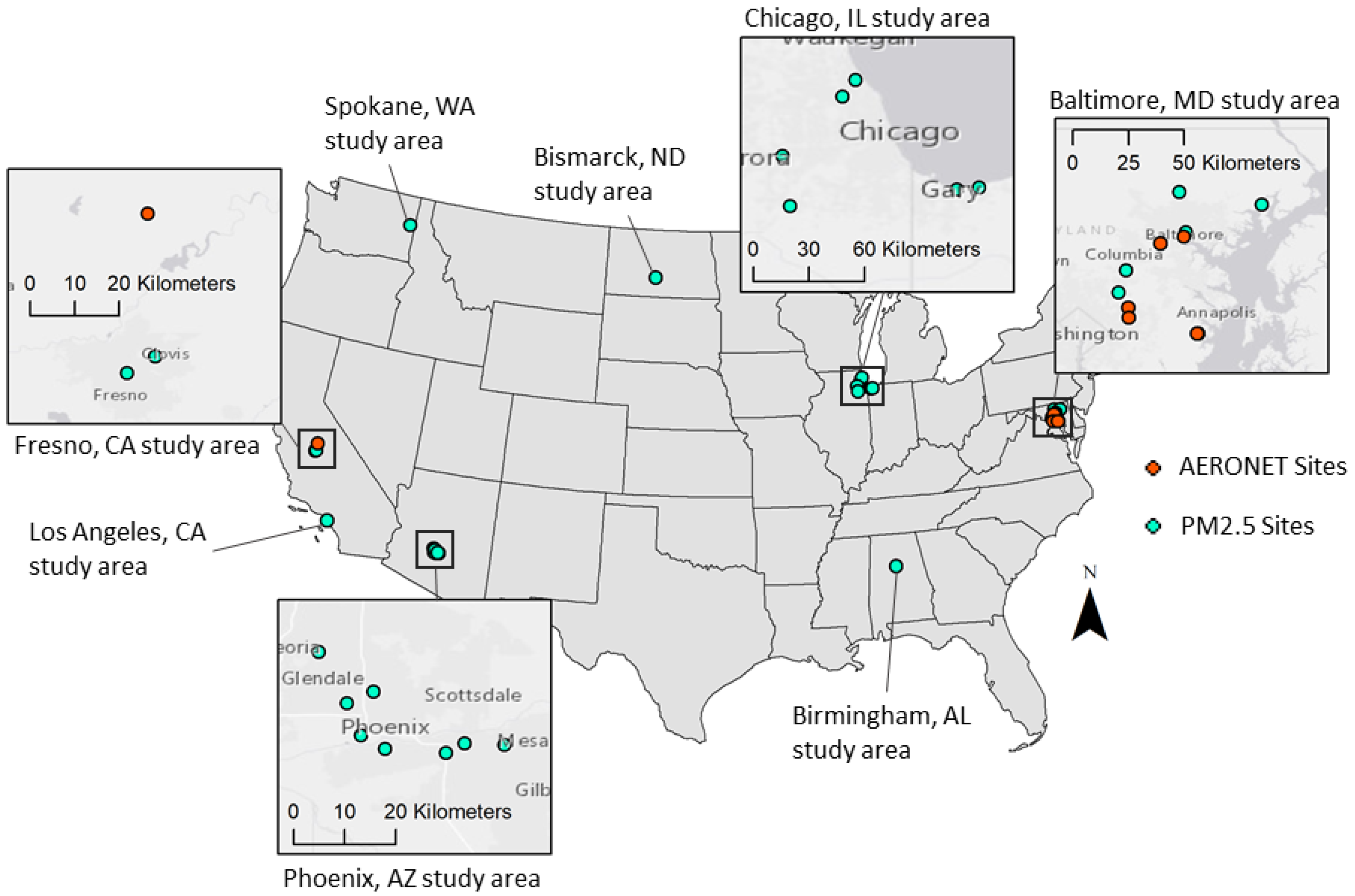
PM2.5 concentration measurements collected from EPA AQS ground monitors were used for this study. Only monitors providing hourly PM2.5 data, and that had data co-located spatially and temporally with the PlanetScope and MODIS data listed in Table 2, were considered. Figure 1 shows the location of the 25 AQS PM2.5 monitors that met the criteria to be used in this study.
2.4. AOD Data
Ground-based AOD were obtained from the AErosol RObotic NETwork (AERONET). Version 3.0 quality level 2.0 AOD data were obtained (https://aeronet.gsfc.nasa.gov/, accessed 16 June 2020). AERONET sites used in this study are summarized in Table 3 and can also be seen in Figure 1. Only monitors that had data available co-located spatially and temporally with the PlanetScope and MODIS imagery from Table 2 were considered.
AERONET measures atmospheric optical parameters approximately every 15 min at wavelengths ranging from 340 nm to 1020 nm [75]. For this study, measurements at wavelengths most closely corresponding to PlanetScope and MODIS spectral bands were used for comparison. These bandwidths are summarized in Table 4.
2.5. Geolocation Comparison
One method for determining geolocation accuracy of satellite data is via ground control points (GCPs). GCPs may be natural or fabricated features on the surface of the Earth that can be easily and precisely identified at the satellite imagery resolution, and which have high-quality (e.g., sub-meter accuracy) location coordinates. Calculating the distance between the coordinates of the GCP in satellite imagery and the known GCP location yields a measure of geolocation accuracy. Ideally, GCPs should cover a variety of land cover types and latitudes to provide a comprehensive measure of accuracy [76]. In the absence of high-quality GCPs, a measure of geolocation accuracy can be attained by comparing satellite imagery to imagery from another satellite or airborne source with a known location accuracy. In fact, this is a method that Planet employs, reporting the use GCPs derived from 2.5 m ALOS base map imagery to assess the geolocation accuracy of PlanetScope data over most of the Earth’s land mass [77]. National Agriculture Imagery Program (NAIP) 1-m resolution imagery, which has an accuracy of 6 m at a 95% confidence interval, is used to identify GCPs for PlanetScope imagery over the United States, and Landsat-8 data is used “as a fallback solution over remote polar areas and some small islands” [77,78].
High quality GCPs and high-resolution satellite imagery with a known geolocation accuracy were not available for this study. Therefore, base map imagery from ArcMap (Version 10.5.1) was used as a best-available alternative to assess the geolocation quality of PlanetScope data. ArcMap is a commercial geographic information system (GIS) software produced by ESRI that uses high-resolution data from a variety of sources to create its base map layer. The sources of the base map imagery are cited within the software and include the spatial resolution of the underlying imagery as well as the reported spatial accuracy. Ten control points were selected for the PlanetScope data covering each study area (Table 2), and each control point was manually compared to ArcMap’s base map imagery. Any features in the PlanetScope imagery that appeared shifted from the base map were investigated further and for these features, the approximate distance between the control point feature in the PlanetScope image and the base map were measured. Since Planet reports a geolocation accuracy of 10 m, discrepancies measuring greater than 10 m were noted. The goal of this method was to use a common reference point (i.e., the ArcMap base map imagery) in order to identify shifts in PlanetScope imagery acquired between the two different dates in each study area. Alignment of the imagery from both dates with the base map indicate that the PlanetScope imagery geolocation is consistent between the two dates and can be compared. If there is a significant offset for one or both dates of the PlanetScope imagery, then further geolocation correction may be warranted to ensure imagery from both dates are aligned as closely as possible. Since ArcMap base map imagery are compiled from different sources, this methodology only provides a measure of geolocation consistency between the multi- source base map imagery and PlanetScope data from two select dates. Nonetheless, agreement between all imagery sources at the same location is a positive indicator of geolocation accuracy. A summary of the ArcMap base map imagery intersecting each control point surveyed, as well as the cited accuracy for each, are summarized in Appendix A Table A1. The spatial resolution of the ArcMap base map imagery ranged from 0.07 m with a geolocation accuracy of ±0.73-m, to 0.5 m with a geolocation accuracy of ±5 m.
2.6. Comparison of PlanetScope and MODIS Spectral Signatures over Different Land Cover Types
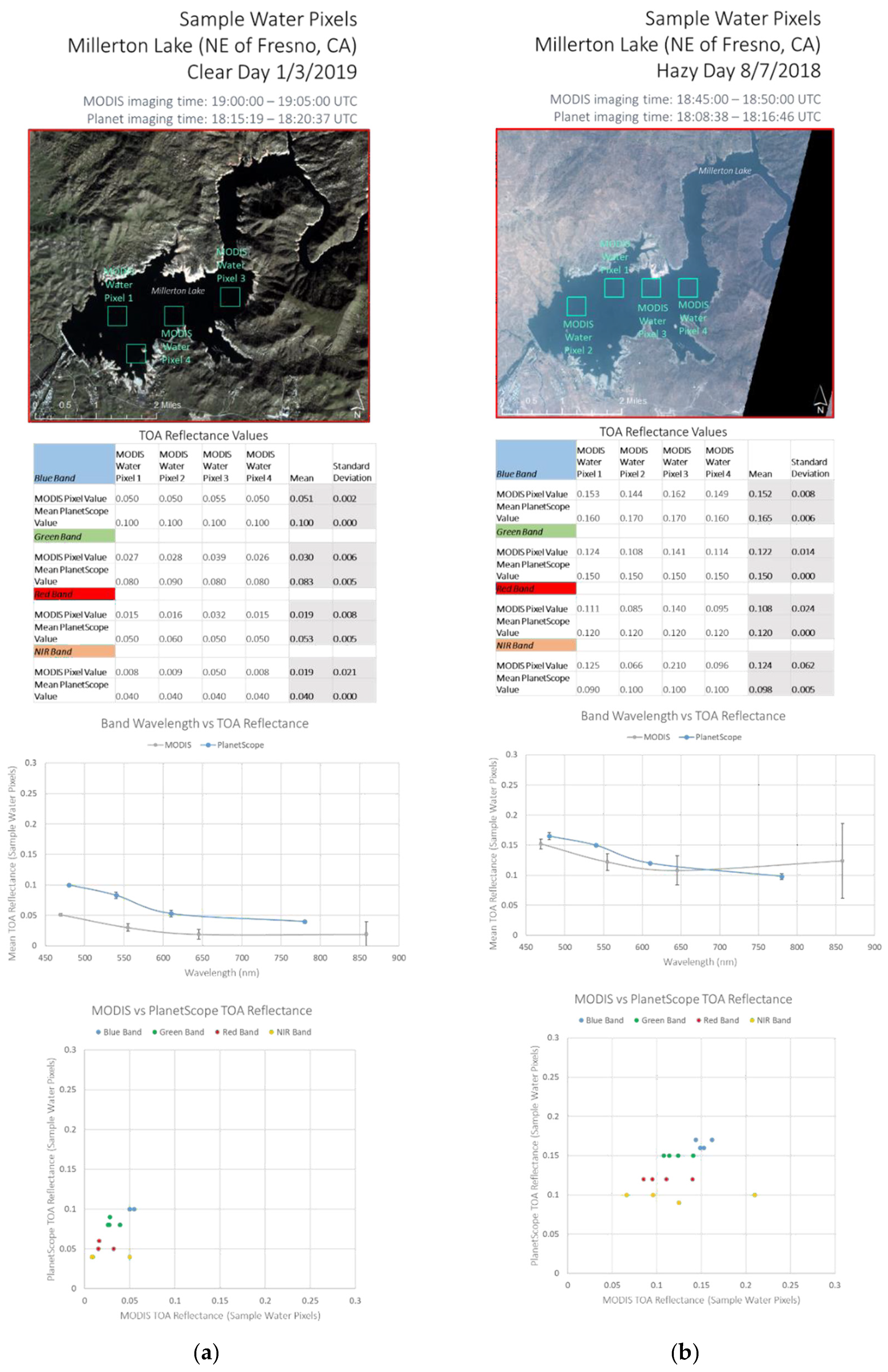
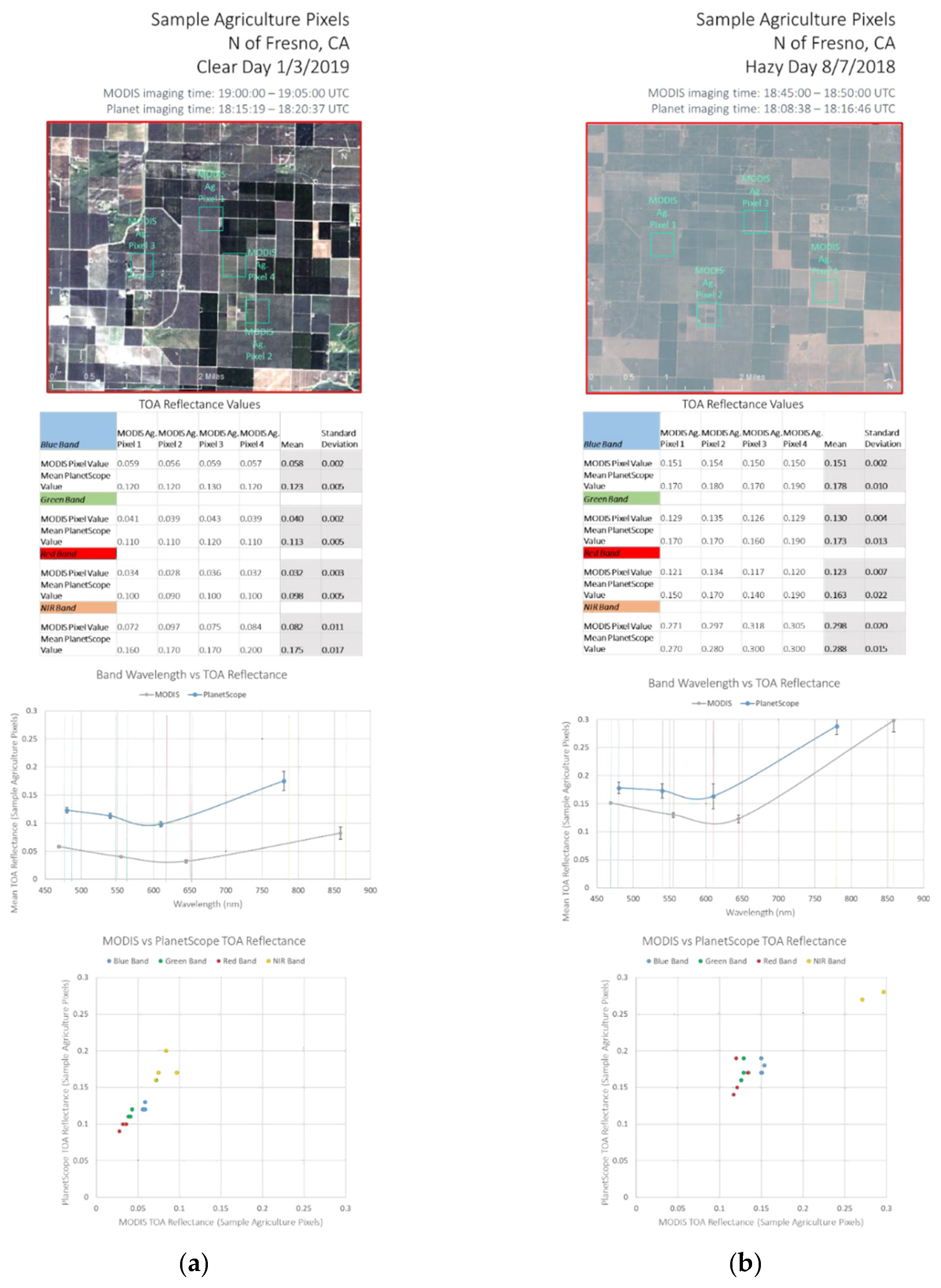
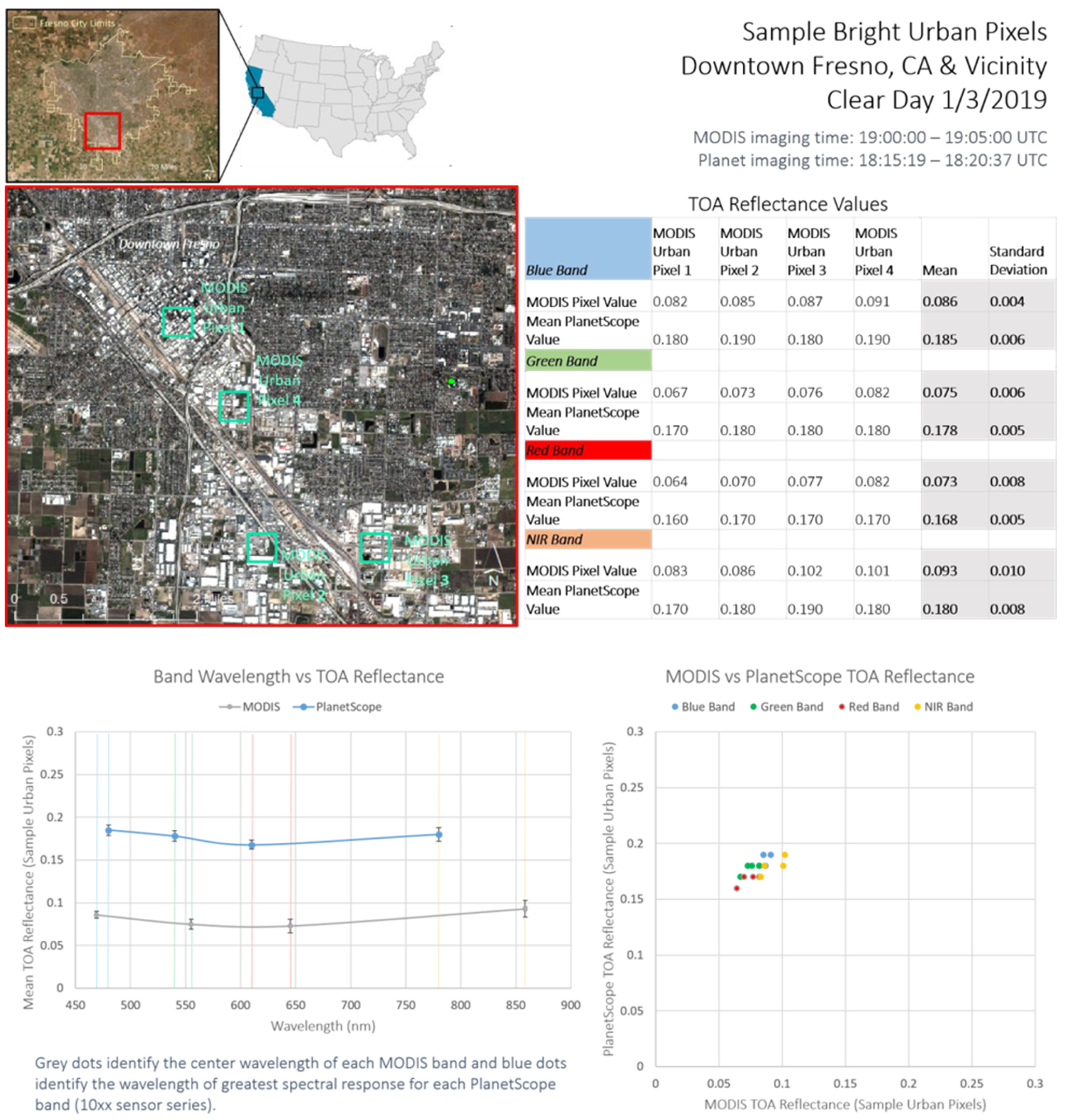
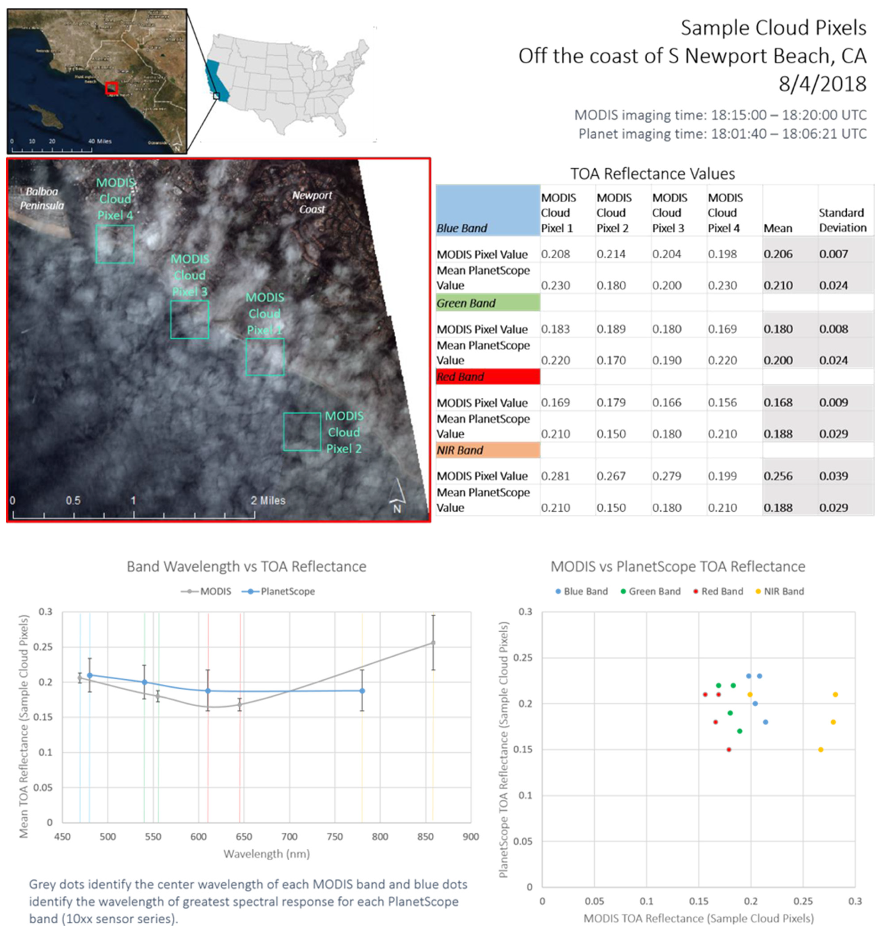
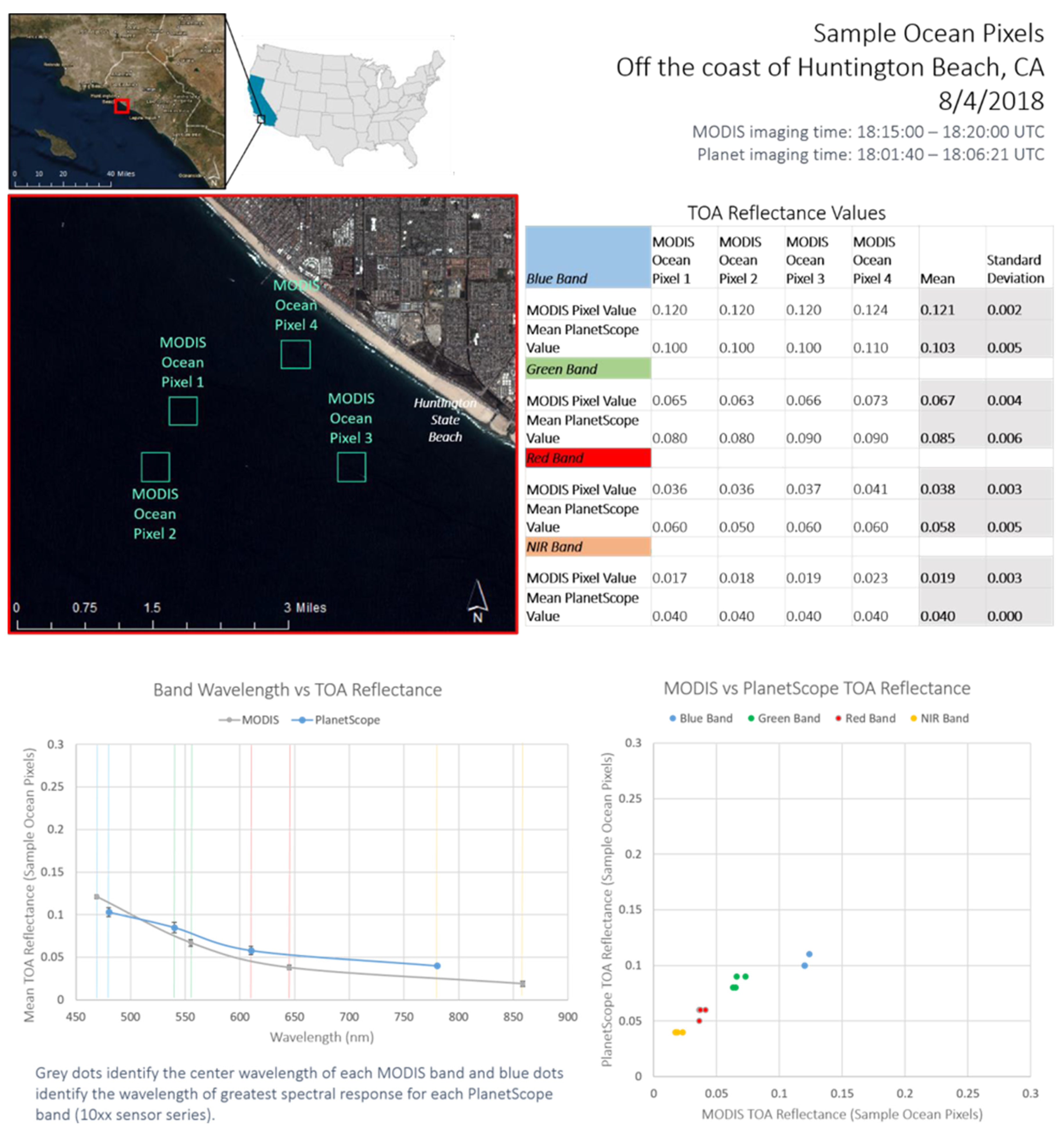
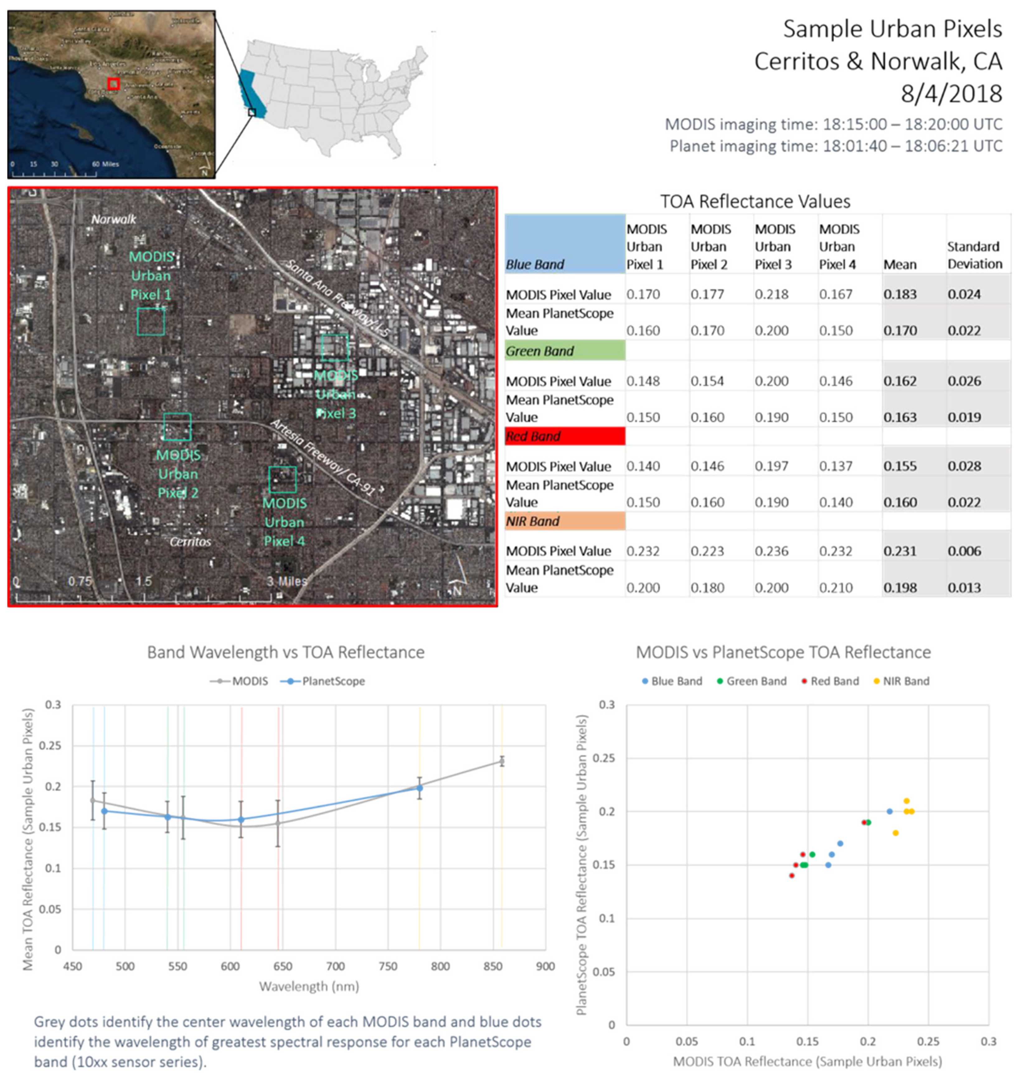
The Fresno, CA study area (Table 2) was more closely inspected to compare the spectral signatures, in terms of TOA reflectance, from PlanetScope and MODIS over a variety of land cover types including an inland freshwater lake, urban areas, and agricultural land. For the fresh water and agricultural land cover types, a comparison was also done between PlanetScope and MODIS for a clear (1/3/2019) and a hazy (8/7/2018) day, to assess how TOA reflectance varies over the same land cover type but under differing air quality conditions. Imagery from the Los Angeles study area (Table 2) were also inspected for the inclusion of additional land cover types. Samples from the Los Angeles study area include cloudy pixels, ocean water, and an additional urban area sample. Combined, these samples cover a range of reflectance values. Maps detailing the location of each land cover type surveyed are included in Appendix A Figure A1, Figure A2, Figure A3, Figure A4 and Figure A5.
Four MODIS pixels (500 × 500 m) were randomly selected over each land cover type. For each pixel, the TOA reflectance value for MODIS bands 1–4 (red, NIR, blue, green) were recorded. For the corresponding PlanetScope imagery, the mean TOA reflectance of all PlanetScope pixels falling within the extent of each 500 m MODIS pixel were recorded for comparison. This was done for each PlanetScope band (blue, green, red, NIR). Since PlanetScope pixels are at a 3 m resolution, approximately 27,778 PlanetScope pixels fall within the extent of a single MODIS pixel. The mean and standard deviation of the TOA reflectance of the four randomly selected pixels were calculated and recorded for each band over each land cover type.
2.7. Analysis of PlanetScope and MODIS Spectral Response to Varying Surface PM2.5 Conditions
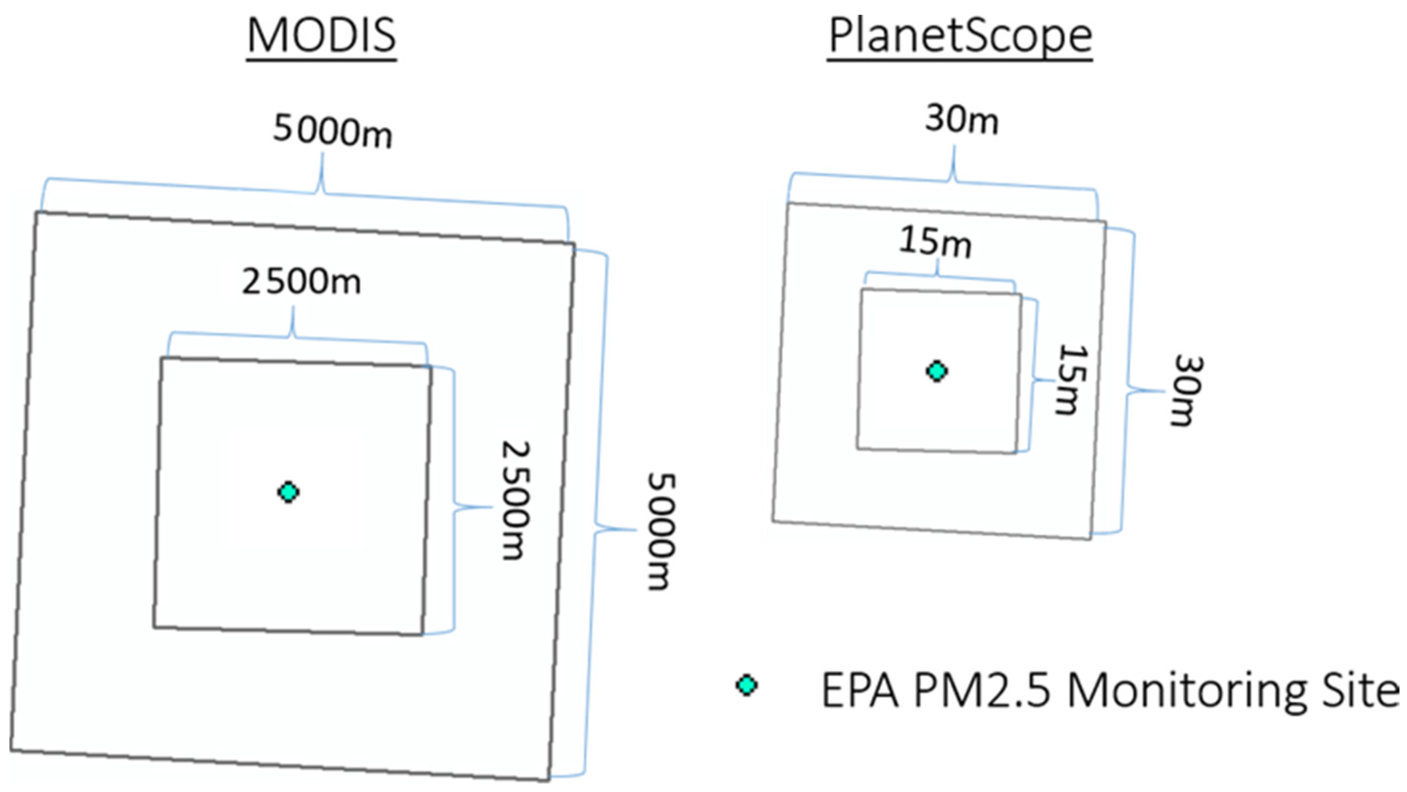
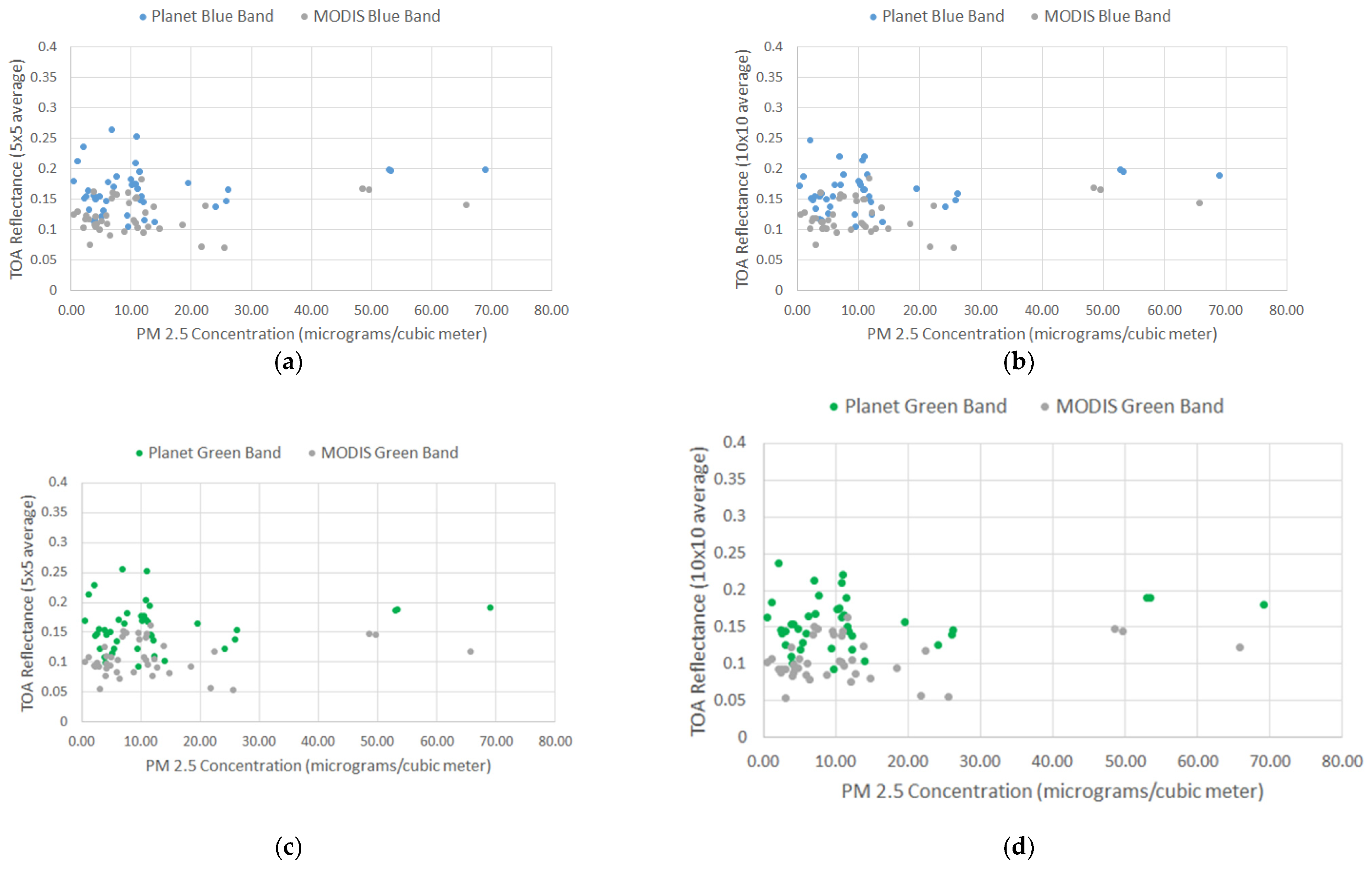
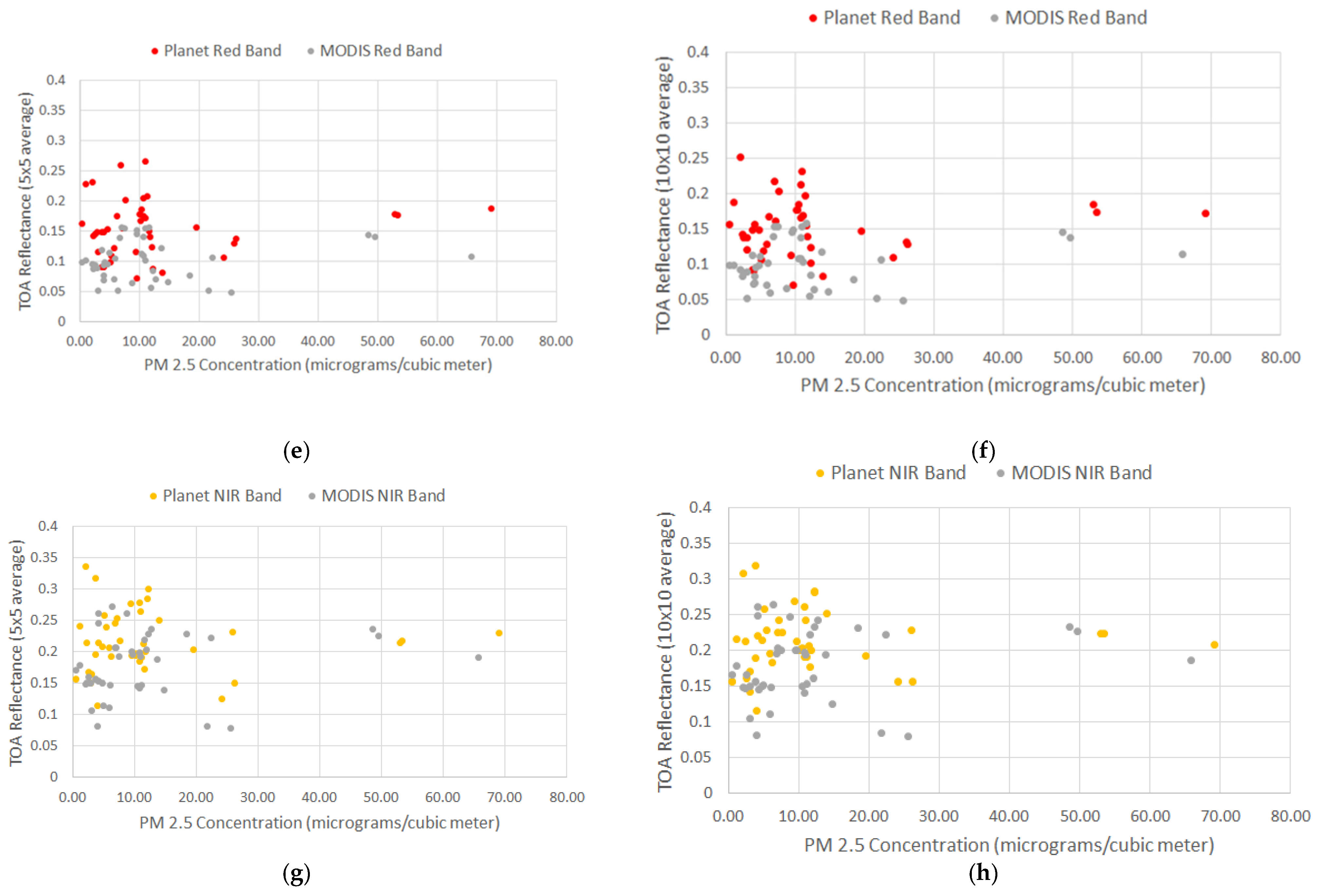
The TOA reflectance values for corresponding PlanetScope and MODIS imagery (Table 2) were averaged over a 5 × 5 and 10 × 10 pixel-sized box centered around each PM2.5 ground monitoring site shown in Figure 1. For MODIS, a 5 × 5 box measures 2500 m by 2500 m and a 10 × 10 box measures 5000 m by 5000 m (Figure 2). For PlanetScope, a 5 × 5 box measures 15 m by 15 m and a 10 × 10 box measures 30 m by 30 m (Figure 2).
TOA reflectance was averaged over an area surrounding each PM2.5 monitoring site, at two different scales, in order to account for noise in the imagery, and to investigate the effect of scale on the average reflectance value. PM2.5 readings at the EPA AQS monitoring sites used in this study are taken each hour. To account for spatial gradients in the PM2.5 value, the PM2.5 concentrations were averaged over a three-hour window centered as closely as possible to the respective PlanetScope and MODIS image acquisition times. A total of 41 data points were collected, where a data point consists of the 5 × 5 and 10 × 10 averaged TOA reflectance (centered around a PM2.5 station) for an overlapping PlanetScope and MODIS image pair, and the corresponding three-hour averaged PM2.5 concentrations.
2.8. Analysis of PlanetScope and MODIS Spectral Response to AOD
A similar process was repeated for AOD, where TOA reflectance from PlanetScope and MODIS were averaged for a 5 × 5 and 10 × 10 pixel-sized box centered around each AERONET site listed in Table 3. AOD readings for the wavelengths specified in Table 4 were averaged for a three-hour window centered around the respective PlanetScope and MODIS image acquisition times. A total of 10 unique data points were collected, where a unique data point includes 5 × 5 and 10 × 10 averaged TOA reflectance for an overlapping PlanetScope and MODIS acquisition (obtained within 70 min of one another), centered around an AERONET site, along with the corresponding three-hour averaged AERONET AOD.
3. Results
3.1. Geolocation Comparison
Overall, the surveyed control points showed good co-location between the PlanetScope imagery and ArcMap base map imagery. Nine of the eighty control points surveyed had an offset approximated to be between 6–10 m (i.e., greater than two pixels). This offset was not consistent across all surveyed control points or even across imagery from the same PlanetScope overpass. For some control points, it was difficult to discern the exact offset due to sun-angle and shadow effects in the imagery. Nonetheless, none of the control points appeared to have an offset significantly greater than 10 m, and therefore confirming the geolocation accuracy reported by Planet. Imagery over the Spokane, Phoenix, Los Angeles, Fresno and Chicago study areas had zero or very minimal (less than a pixel) offset estimates. This not only confirms prior results but also provides an independent assessment of geolocation accuracy over multiple locations and time periods. The imagery over Bismarck, Birmingham, and Baltimore contained the nine control points estimated to have an offset greater than 6 m (i.e., two pixels). In most cases, the PlanetScope data appeared to be shifted slightly east or southeast of the control points. Overall, these results suggest that PlanetScope data are accurate within 3–4 pixels, but this result is based on a comparison with ArcMap base map imagery which has a varying degree of accuracy depending on the source data. The lowest accuracy cited in the base map imagery metadata was 5 m (i.e., nearly 2 PlanetScope pixels) at a 0.5 m resolution, adding an uncertainty of 5 m to the results (Table A1). Based on the results of the geolocation comparison, additional geolocation correction was not pursued for the PlanetScope data used in this study. Given the number and variety of these smallsats, we recommend that users perform an independent assessment of geolocation accuracy before conducting scientific studies.
3.2. Comparison of PlanetScope and MODIS Spectral Signatures over Different Land Cover Types
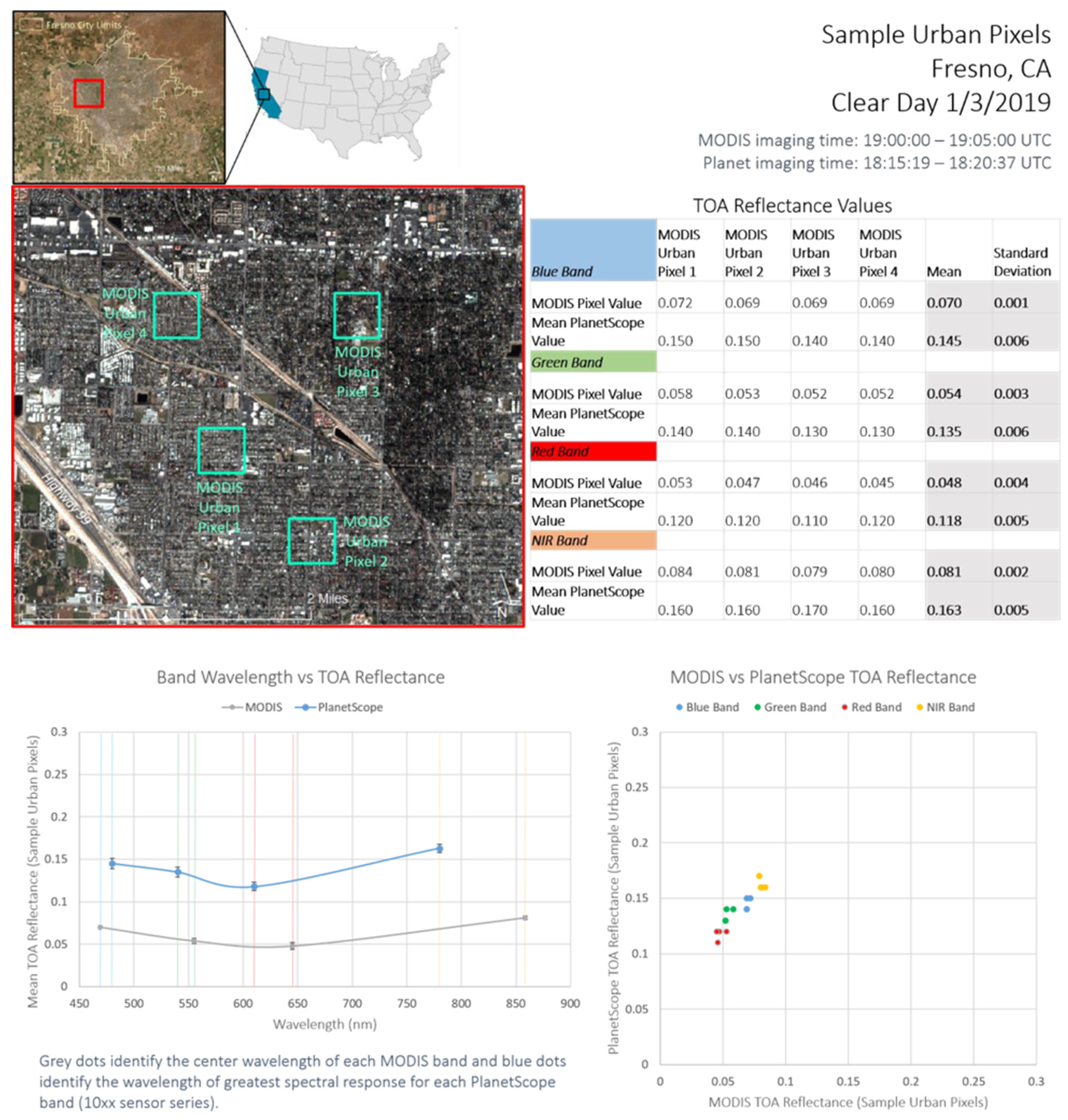
Spectral signatures are perhaps one of the fundamental ways to assess how the reflectance of various classes (e.g., clouds, vegetation) vary as a function of reflectance. This is often used in various supervised classification techniques to separate pixels into one of many classes. Also, selection of training samples are used in a wide variety of studies including machine learning techniques. The third row of Figure 3 and Figure 4 (continued in the Appendix A Figure A1, Figure A2, Figure A3, Figure A4 and Figure A5) show the mean TOA reflectance, for both PlanetScope and MODIS, of the four randomly sampled MODIS pixels plotted as a function of wavelength. The wavelength of the greatest spectral response for the 10xx PlanetScope sensor series is used as the wavelength on the x-axis for PlanetScope, and the center wavelength of each MODIS band is used as the wavelength on the x-axis for MODIS. The standard deviation of the four pixels used to calculate the mean TOA reflectance are also shown.
Across all samples taken over the Fresno study area, the mean TOA reflectance from PlanetScope trends slightly higher (by 0.06 on average) than that of the compared MODIS pixel across all four bands, with the exception of the Millerton Lake hazy day sample (Figure 3b). For the three land cover types sampled over the Los Angeles study area, the spectral signatures for PlanetScope and MODIS trend closer together in comparison (average difference in reflectance of 0.02). A total of 12 samples were taken over the Los Angeles study area, and for these samples the mean difference in TOA reflectance between PlanetScope and MODIS was 0.018 ± 0.009 for the blue band (RMSE 0.020), 0.018 ± 0.014 for the green band (RMSE 0.022), 0.021 ± 0.015 for the red band (RMSE 0.025), and 0.043 ± 0.034 for the NIR band (RMSE 0.054). A total of 24 samples were taken over the Fresno study area, and for these samples the mean difference in TOA reflectance between PlanetScope and MODIS was slightly higher at 0.054 ± 0.030 for the blue band (RMSE 0.062), 0.059 ± 0.027 for the green band (RMSE 0.062), 0.054 ± 0.027 for the red band (RMSE 0.060), and 0.057 ± 0.037 for the NIR band (RMSE 0.068). The closer agreement between PlanetScope and MODIS TOA reflectance for the Los Angeles study area could be attributed to the difference in image acquisition time being only ~15 min, compared to ~30–40 min for the Fresno samples.
A total of 36 samples were taken across both the Fresno and Los Angeles study areas. Across all samples, the mean difference in TOA reflectance was 0.042 ± 0.030 for the blue band (RMSE 0.052), 0.045 ± 0.027 for the green band (RMSE 0.052), 0.043 ± 0.028 for the red band (RMSE 0.051), and 0.052 ± 0.037 for the NIR band (RMSE 0.064). The TOA reflectance was higher for PlanetScope compared to MODIS for 72% of the blue band samples, 94% of the green band samples, 92% of the red band samples, and 61% of the NIR band samples. While the TOA reflectance from the PS2 sensor trends slightly higher than MODIS overall, the results could be affected by the small sample size. The offset in image acquisition time between PlanetScope and MODIS, as well as the differences in spectral response functions between the two sensors, are also factors that are expected to contribute to some difference in TOA reflectance.
The fourth row of Figure 3 and Figure 4 (continued in Appendix A Figure A1, Figure A2, Figure A3, Figure A4 and Figure A5) also shows the results as scatter plots with the reflectance of each sampled MODIS pixel on the x-axis, and the mean reflectance of the corresponding PlanetScope pixels on the y-axis. Values from each spectral band are color coded. Tighter clusters of the same color indicate less variability in reflectance across the sampled pixels. The reflectance values generally behave as expected. For instance, the samples over bodies of water show the lowest reflectance in the NIR band, which is expected since water absorbs large amounts of NIR light (Figure 3a,b and Figure A4). Reflectance is high across all bands for the sampled cloudy pixels, which is expected since clouds scatter light in the visible wavelengths as well as the NIR range covered by PlanetScope and MODIS NIR bands (Figure A3; [79]). All samples over urban areas show the highest reflectance in the NIR, followed by blue, green, and red, and the cluster of points is the tightest for pixels sampled over urban areas with many similar, highly reflective buildings (Figure A1). In the Fresno study area, samples were taken over an inland body of water, Millerton Lake, for both a relatively clear day (1/3/2019) and a hazy day (8/7/2018), in order to compare TOA reflectance under the same surface conditions but under differing atmospheric conditions (Figure 3). The haze seen in the 8/7/2018 imagery can be primarily attributed to the nearby Ferguson wildfire that burned approximately 392 km2 of land north of Fresno in the Sierra and Stanislaus National Forests and Yosemite National Park between 13 July and 19 August 2018 (Figure 3b and Figure 4b). As expected, the reflectance is higher across all PlanetScope and MODIS bands on the hazy day, due to the added aerosols in the atmosphere from the smoke. The cluster of points also appears to be more spread apart on the hazy day. This could be due to the influence of a variety of aerosols in the atmosphere.
Clear and hazy day samples were also compared over an area of agricultural land located north of Fresno’s city center (Figure 4). TOA reflectance similarly increased across all bands for both PlanetScope and MODIS on the hazy day, with the greatest increase in reflectance seen in the NIR bands (Figure 4b). Since the clear day sample was taken in January and the hazy day sample in August, seasonal changes may contribute to some of the reflectance differences observed. Additionally, the pixels were sampled over the same geographical area but do not overlap exactly between the clear and hazy day samples, which may also contribute to some variability in reflectance.
3.3. Analysis of PlanetScope and MODIS Spectral Response to Varying Surface PM2.5 Conditions
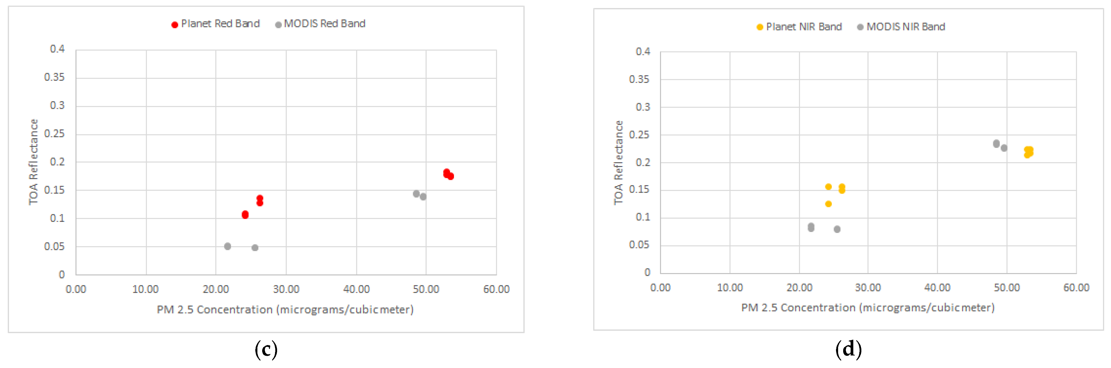
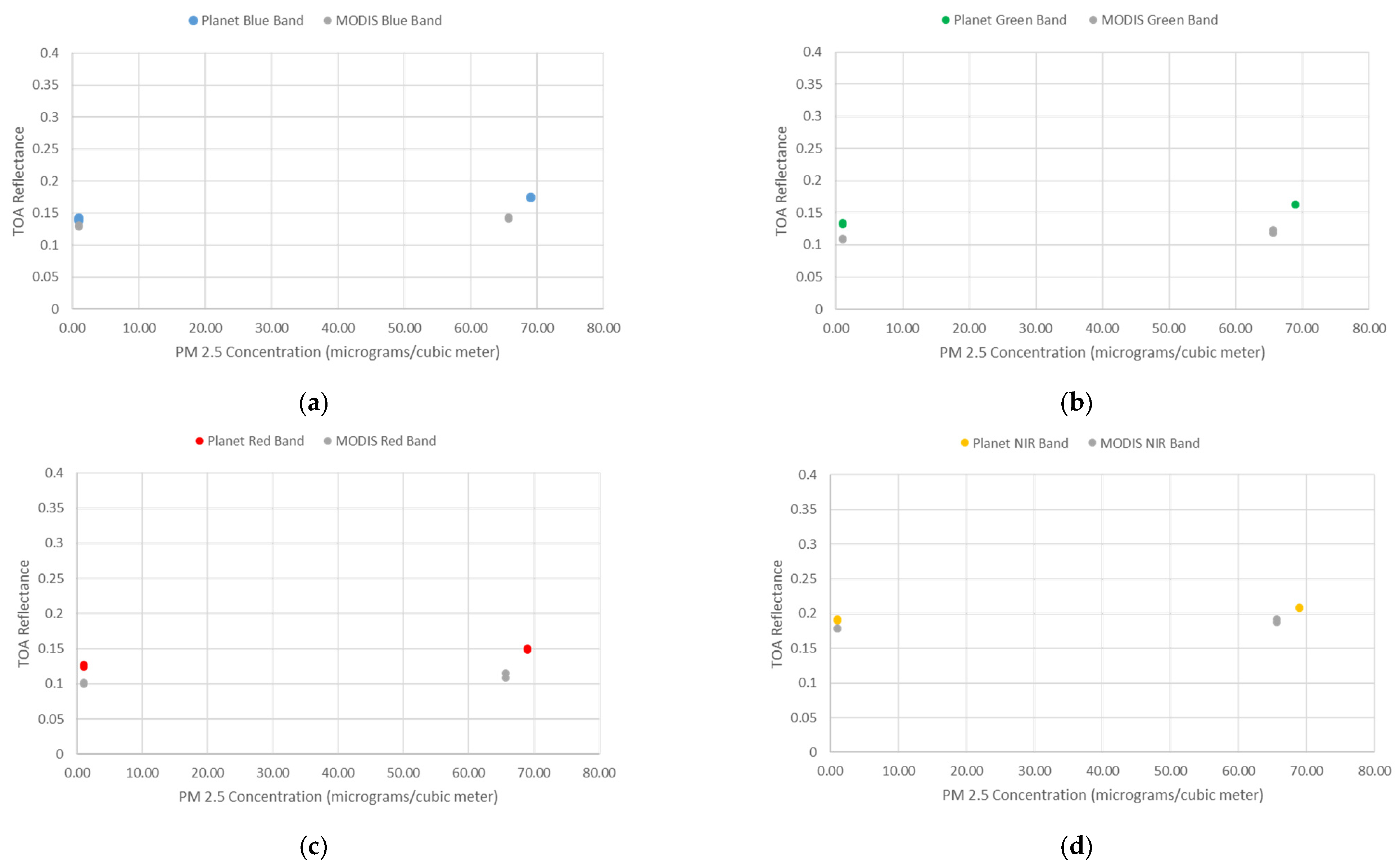
Figure 5 shows scatter plots of PlanetScope and MODIS TOA reflectance in relation to PM2.5 concentrations at 25 different PM2.5 ground monitoring locations. Typically, visible surface reflectance that is used to retrieve AOD in satellite algorithms should be correlated with surface PM2.5 provided the aerosols are closer to the surface with known aerosol properties [51]. Retrieval of AOD from satellite imagery is complicated because it involves the use of a radiative transfer algorithm and various assumptions of aerosol, surface, and atmospheric properties. Our future research will use PlanetScope data and radiative transfer algorithms to retrieve AOD and then validate with AERONET and compare with surface PM2.5. In this paper, we use the TOA reflectance as an exploratory surrogate for AOD. Data were collected for 15 different dates over eight U.S. cities. For each study area, two dates were selected to capture a variety of air quality conditions. The x-axis shows the average PM2.5 concentrations for a three-hour period centered around the PlanetScope/MODIS image acquisition time. The y-axis shows PlanetScope and MODIS TOA reflectance averaged for a 5 × 5 or 10 × 10 pixel sized box centered around each PM2.5 station location. The 5 × 5 plots are shown in the left-hand column of Figure 5, and the 10 × 10 average plots are shown in the right-hand column. Data points from MODIS are shown in grey while data points from PlanetScope are shown in color. The average reflectance of the pixels surrounding each PM2.5 site were used to account for noise as well as potential geolocation errors in the case of PlanetScope.
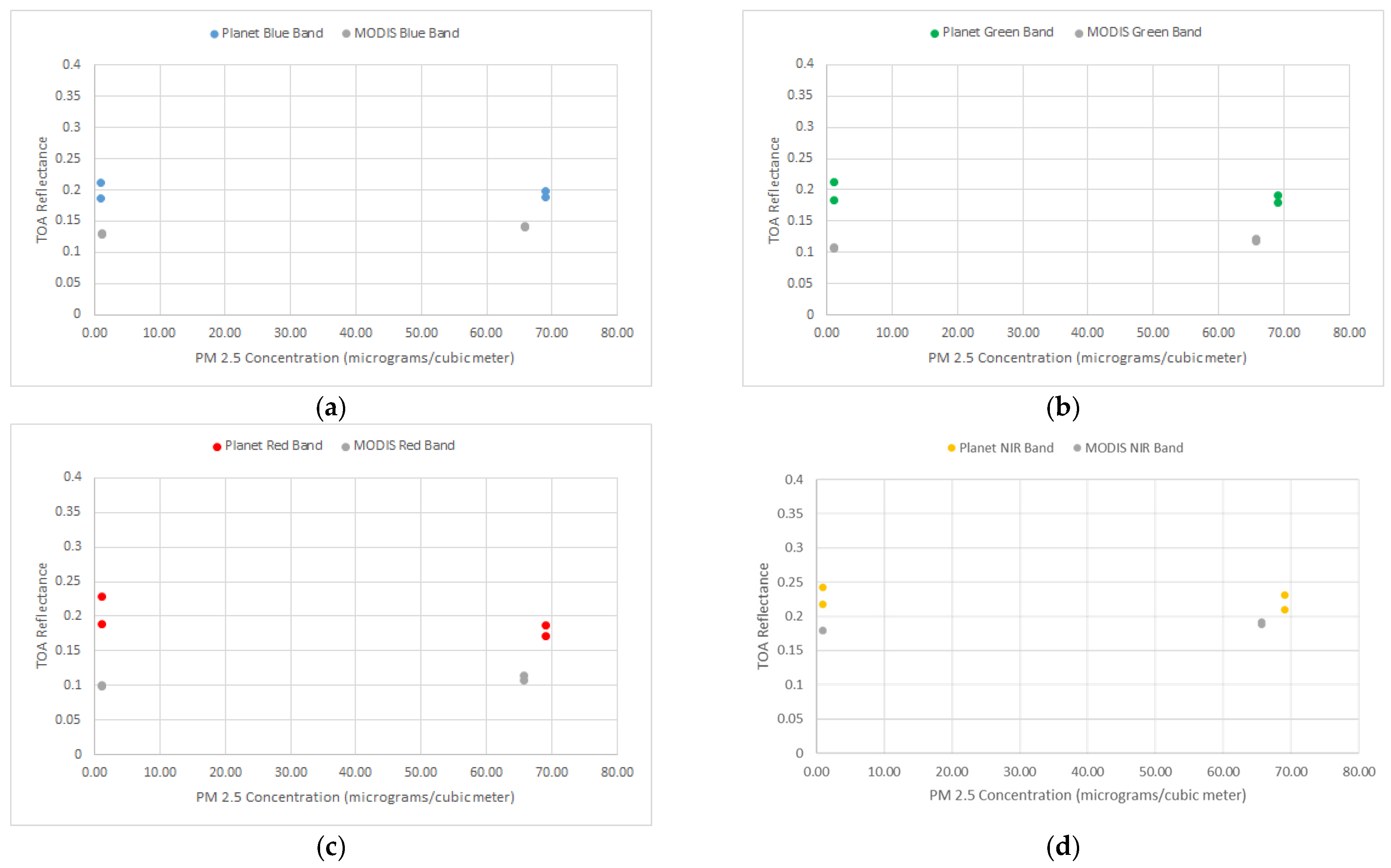
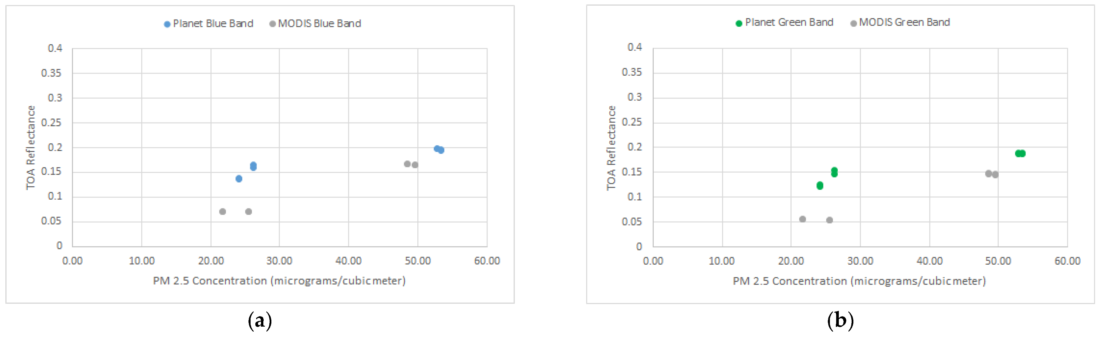
PM2.5 concentrations in the scatter plots range from 0.37 to 69 µg/m3. In order to meet current EPA standards, PM2.5 concentrations should remain less than or equal to 35 μg/m3 over a 24-h averaged time period. This threshold was exceeded at the Fresno—Garland and Clovis PM2.5 stations sampled on 8/7/2018 as well as the SPOKANE—AUGUSTA AVE station sampled on 8/14/2018. The high PM2.5 readings at these locations can be attributed to nearby wildfire events, including the Ferguson wildfire near Fresno and smoke from local and nearby Canadian wildfires that resulted in unhealthy PM2.5 levels in Spokane. These poor air quality days are visible as small clusters in the right-hand side of the scatter plots. The scatter plots show no apparent correlation between PM2.5 and TOA reflectance. This is not a cause for concern since many factors influence the TOA reflectance signal, including land surface reflectivity, vertical distribution of aerosols, the geographic region, and aerosol type [51]. The points in the scatter plot include samples from a variety of geographic regions, land cover types, times of year, and atmospheric conditions, all of which contribute to the TOA reflectance signal to a varying degree. This is further illustrated by isolating the samples from a clear and extremely hazy day at the same location. Figure 6 isolates the data points from both the 5 × 5 and 10 × 10 scatter plots for the SPOKANE—AUGUSTA AVE station, which saw very low PM2.5 on 4/19/2018 and high PM2.5 on 8/14/2018 due to nearby wildfires.
Even with the large difference in PM2.5 concentration, the difference in TOA reflectance is minimal across all bands, indicating that PM2.5 is not the primary factor accounting for changes in TOA reflectance between these two dates. It is important to note that there does appear to be a very slight increase in TOA reflectance for MODIS across all bands, but the same does not appear to be true for PlanetScope (Figure 6). However, averaging the TOA reflectance for PlanetScope over the same spatial area as MODIS (i.e., 2500 × 2500 m and 5000 × 5000 m versus 15 × 15 m and 30 × 30 m) does result in a noticeable increase in TOA reflectance on the high PM2.5 day (Appendix A Figure A6). Nonetheless, isolating the data points from the Fresno study area paints a different picture (Figure 7).
Here, there is an even more pronounced increase in TOA reflectance on the high PM2.5 day compared to the lower PM2.5 day for both PlanetScope and MODIS. This indicates that, perhaps, PM2.5 had a somewhat larger influence on the TOA reflectance signal at the Fresno sites between the clear and hazy days sampled. The examples highlighted in Figure 6 and Figure 7 speak to the complexities involved in accurately modeling the relationship between satellite data and PM2.5.
For both the 5 × 5 and 10 × 10 plots, PlanetScope reflectance trends slightly higher than MODIS (with the most visible overlap in the NIR band), which aligns with the results from Section 3.2. Across all 5 × 5 samples, the mean difference between PlanetScope and MODIS reflectance was 0.044 ± 0.032 for the blue band, 0.052 ± 0.032 for the green band, 0.053 ± 0.035 for the red band, and 0.047 ± 0.036 for the NIR band. Across all 10 × 10 samples, the mean difference between PlanetScope and MODIS reflectance was 0.042 ± 0.028 for the blue band, 0.051 ± 0.027 for the green band, 0.052 ± 0.029 for the red band, and 0.044 ± 0.034 for the NIR band. Across both the 5 × 5 and 10 × 10 plots, PlanetScope reflectance was higher than the corresponding MODIS reflectance 91% of the time. Across both the 5 × 5 and 10 × 10 plots, the points with the smallest difference in reflectance had a discrepancy in image acquisition time ranging from approximately 7–19 min, compared to a discrepancy ranging from 42–58 min for the points with the largest difference in reflectance. This suggests, as would be expected, that the agreement between PlanetScope and MODIS improve if the imagery is acquired closer to the same time. As mentioned in Section 3.2, some difference in reflectance is also expected due to PlanetScope’s wider spectral bandwidths compared to MODIS (Table 4). It is important to note that some difference in reflectance is also expected due to the considerable difference in PlanetScope and MODIS pixel size. A 5 × 5-pixel sized area for MODIS covers 2500 m2 compared to only 15 m2 for PlanetScope.
The difference in reflectance between the 5 × 5 and 10 × 10 pixel averages for PlanetScope were minimal, with the mean difference in reflectance equaling 0.006 ± 0.009 for the blue band, 0.007 ± 0.008 for the green band, 0.008 ± 0.010 for the red band, and 0.009 ± 0.008 for the NIR band. The difference in reflectance between the 5 × 5 and 10 × 10 MODIS pixel averages were even smaller, with the mean difference in reflectance ranging from 0.002 ± 0.002 for the blue and green band, to 0.003 ± 0.002 for the red band and 0.006 ± 0.009 for the NIR band. These results indicate a negligible difference in reflectance for both PlanetScope and MODIS when averaged between a 5 × 5 and 10 × 10 pixel-sized area. If the 5 × 5 values were compared to data averaged over a much larger scale, say 25 × 25 pixels, the difference may have been more pronounced.
3.4. PlanetScope and MODIS Spectral Response to AOD
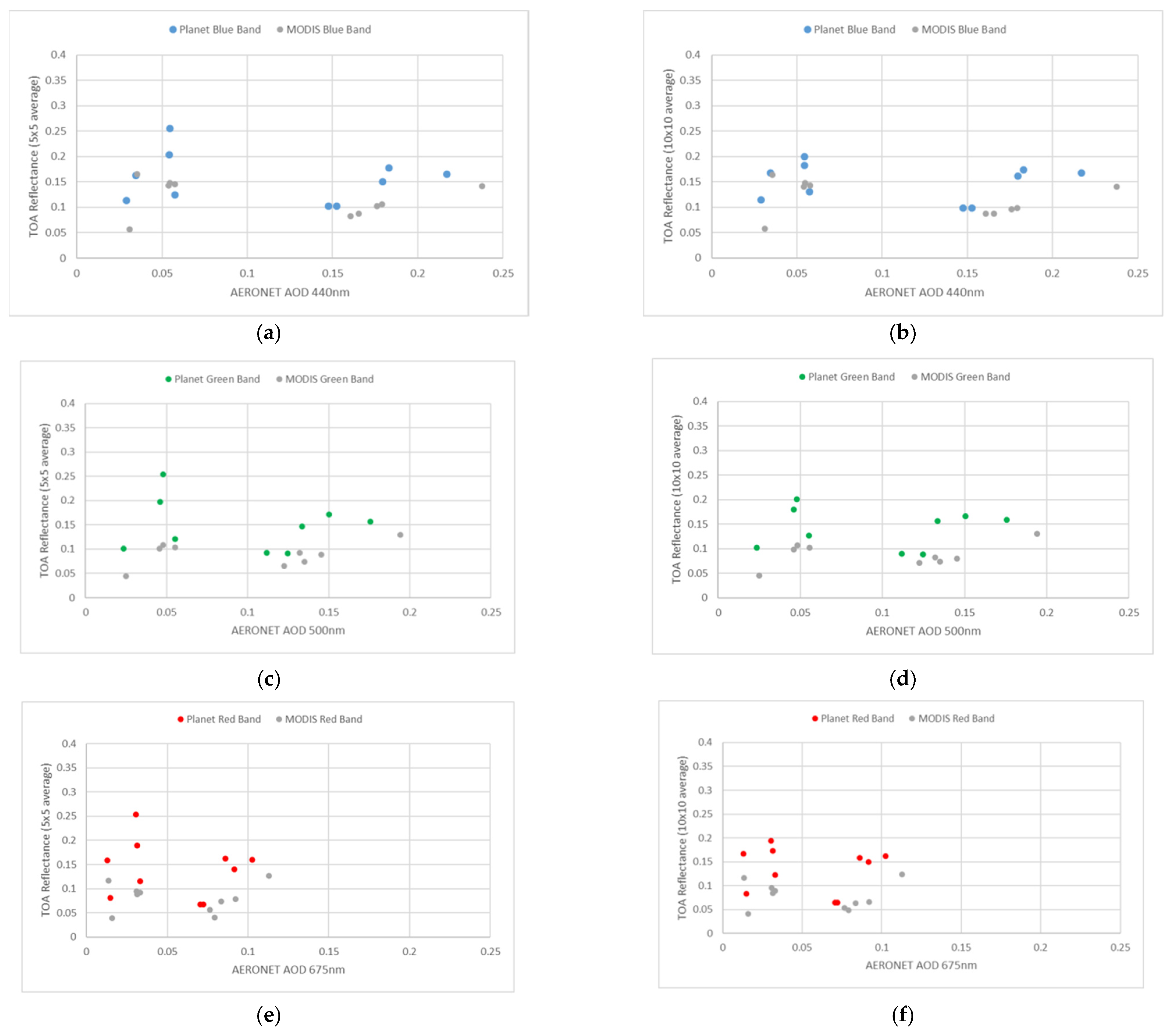
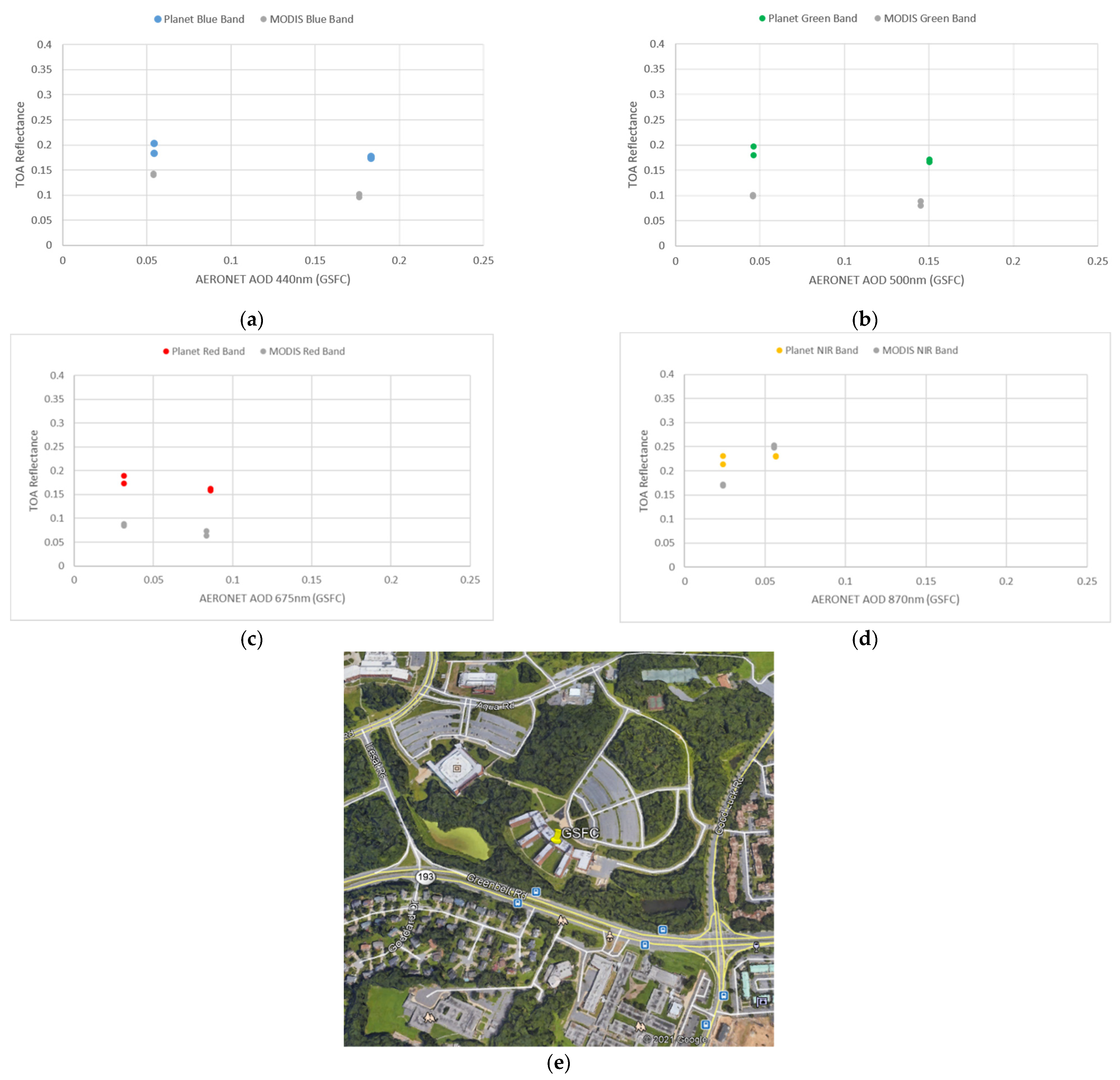
Figure 8 shows scatter plots of PlanetScope and MODIS TOA reflectance in relation to AOD collected at seven AERONET sites over three different dates, resulting in a total of 10 PlanetScope/MODIS point pairs (Table 3). All data summarized in Table 2 were assessed for AERONET data availability. However, only select AERONET sites had data available on the selected study dates, resulting in the small sample size. The sample includes data from six sites in the Baltimore study area and one site from the Fresno study area. The x-axis shows the average AOD for a three-hour time period centered around the PlanetScope/MODIS image acquisition time. The AOD average was calculated for the AERONET band most closely overlapping each PlanetScope/MODIS band (Table 4). The y-axis shows PlanetScope and MODIS TOA reflectance averaged for a 5 × 5 and 10 × 10 pixel sized box centered around each AERONET site. Data points from MODIS are shown in grey while data points from PlanetScope are shown in color. There are two plots for each band, one for the 5 × 5 TOA reflectance average, and one for the 10 × 10 TOA reflectance average.
Plotted AOD values range from 0.008 in the 870 nm channel to 0.238 in the 440 nm channel. The samples with the highest AOD values were collected at the MD_Science_Center AERONET site on 7/14/2018, and the samples with the lowest AOD values were a tie between the MD_Science_Center site on 3/22/2017 and the NEON_SJER site near Fresno on 1/3/2019. The difference in reflectance between PlanetScope and MODIS was 0.042 ± 0.033 for the blue band, 0.056 ± 0.042 for the green band, 0.059 ± 0.045 for the red band, and 0.037 ± 0.028 for the NIR band, averaged across all 5 × 5 samples. Across all 10 × 10 samples, the mean difference in reflectance between PlanetScope and MODIS was 0.036 ± 0.026 for the blue band, 0.052 ± 0.030 for the green band, 0.056 ± 0.033 for the red band, and 0.039 ± 0.015 for the NIR band. 85% of the PlanetScope samples had a higher reflectance than MODIS for the 5 × 5 averages, and 90% of the PlanetScope samples had a higher reflectance than MODIS for the 10 × 10 averages, aligning with the results from Section 3.2. PlanetScope imagery was acquired approximately 47 min before MODIS for the Fresno location on 1/3/2019. PlanetScope imagery was acquired approximately 57–58 min and 16 min before MODIS for the Baltimore sites on 7/14/2018 and 3/22/2017, respectively. Isolating the data points from 3/22/2017, where the image acquisition was only 16 min apart, did not significantly improve the mean difference in reflectance between PlanetScope and MODIS. This could be due to the small sample size or the influence of other factors, such as the difference between PlanetScope and MODIS spectral response, or the scale difference playing a larger role.
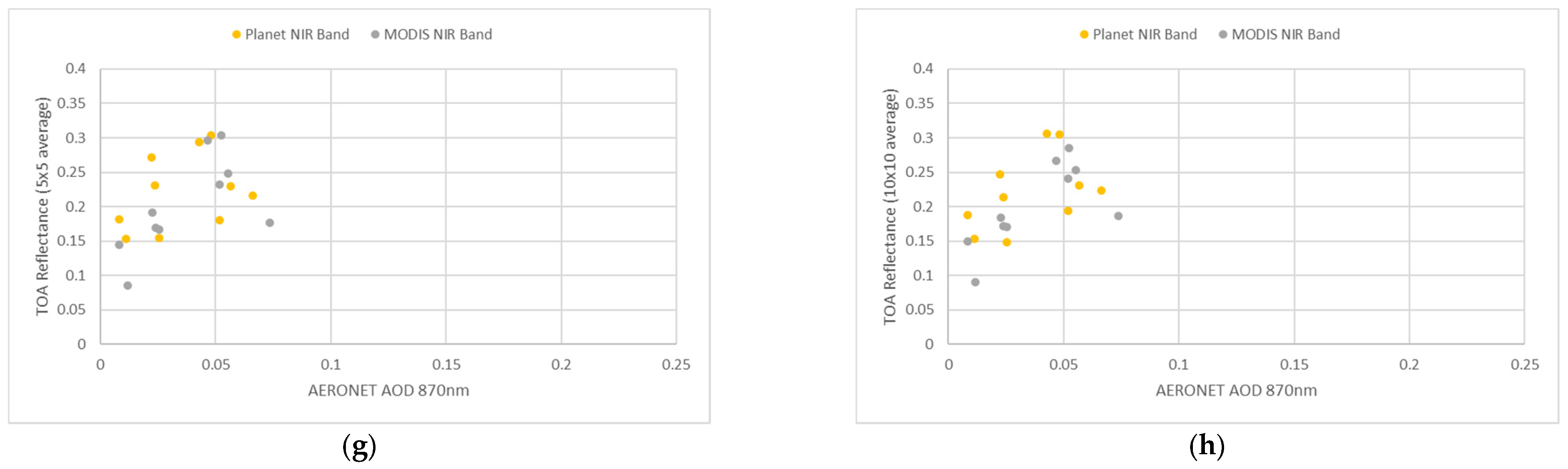
Similar to the results from Section 3.3, there was no significant correlation observed between TOA reflectance and AOD across all samples, especially for low AOD conditions since the surface contribution to the satellite signal is high. The strongest positive linear correlation was for the MODIS NIR band with an r2 of 0.40 for the 5 × 5 pixel average and an r2 of 0.48 for the 10 × 10 pixel average. For the PlanetScope NIR band, in comparison, the r2 was only 0.13 for the 5 × 5 pixel average and 0.22 for the 10 × 10 pixel average. The next highest r2 value was 0.11 for the MODIS green band 5 × 5 pixel average and 0.10 for the 10 × 10 pixel average. The r2 for all other bands, both PlanetScope and MODIS, was 0.06 or less. AOD has been shown to have a positive linear correlation with TOA reflectance when controlled for surface conditions [80]. This relationship holds true even in urban areas (although to a lesser degree) where surface reflectance values tend to be higher and play a more complex role in the TOA reflectance signal [80]. Isolating the data points from a single AERONET site, which assumes the surface conditions are the same, did not improve the correlation between AOD and TOA reflectance (Appendix A Figure A7, Figure A8 and Figure A9). In fact, the MODIS values behaved opposite as expected in some cases (negative linear correlation instead of positive), with the exception of the NIR band. Further investigation with a larger sample size is warranted to determine whether a correlation exists and in order to gain a better understanding of PlanetScope spectral response to AOD.
4. Discussion and Conclusions
Planet’s constellation of CubeSats provides daily global imagery of the Earth’s surface at an orthorectified 3-m resolution, providing excellent spatiotemporal coverage compared to traditional satellites. However, several studies have expressed concern over the radiometric calibration quality of this data, as well as the limited spectral bands offered by the earlier generations of the PlanetScope sensor. Planet is taking steps to address these limitations and continues to infuse newer sensors into the PlanetScope constellation with improved imaging capabilities. Therefore, it is important to continue to assess the fitness of this data for each unique application, especially as Planet’s commercial data becomes more readily available to the scientific community via avenues such as NASA’s CSDA.
Satellite observations have emerged as a promising means to fill the gaps in ground-based air quality monitoring, and Planet’s high-resolution imagery offers the potential to derive air quality parameters, such as PM2.5, at spatial scales localized enough to benefit human health [81]. A large body of research surrounds the estimation of PM2.5 from satellite derived AOD. More recently, machine learning techniques have been used to derive PM2.5 directly from TOA reflectance without the complexities involved in AOD retrieval [73]. In this study, PlanetScope TOA reflectance was examined in the context of air quality research.
First, the PlanetScope data selected for the study, which included Dove-Classic data from 2017–2019 over eight U.S. cities, were compared against high-resolution base map imagery in ArcMap to gauge geolocation consistency. This was prompted by concerns raised in Houberg & McCabe 2018a [11] as well as NASA’s CSDA evaluation report [20]. Based on a visual assessment of control points at each study area, there was not found to be any offset greater than ~10 m compared to base map imagery in ArcMap, aligning with Planet’s reported geolocation accuracy of 10 m RMSE. Based on this result, additional geolocation correction to the PlanetScope data was not performed for this study. Nonetheless, it is recommended that an independent assessment of geolocation accuracy be performed before utilizing PlanetScope data for scientific research. It is important to note that the base map imagery in ArcMap comes from multiple sources with varying degrees of spatial accuracy. The lowest accuracy reported in the metadata for the base map imagery used in the comparison was 5 m at a 0.5 m resolution, adding an uncertainty equivalent to approximately two PlanetScope pixels to the results. It is also important to note that across the control points analyzed, the topography was relatively flat with elevations ranging from 0 m to 804 m, with a difference in elevation of no more than 314 m within a single study area (the only exception being two control points located at 1220 m elevation in the Los Angeles study area). Primarily urban, suburban, and some rural/agricultural areas were sampled. Additionally, the scope of this initial study was only limited to the U.S. Future work should include an assessment of PlanetScope’s geolocation accuracy in comparison to high-quality (e.g., sub-meter accuracy) GCPs over a wider variety of topography in order to gain a better understanding of the geolocation quality of PlanetScope data. Study areas covering a wider variety of land cover classes (such as forested, tropical, and arctic regions) as well as study sites outside of the U.S. should be included in future work.
Next, TOA reflectance from PlanetScope (PS2 sensor only) was compared to MODIS over a variety of land cover types. Some degree of difference was expected due to differences in PS2 and MODIS spectral response functions and the differences in acquisition times (Table 2). MODIS pixels were randomly sampled over each land cover type. The average TOA reflectance of all PlanetScope pixels falling within the extent of each MODIS pixel were used to compare TOA reflectance values. The difference in TOA reflectance ranged from near-zero (0.0014) to 0.117, with a mean difference in reflectance of 0.046 ± 0.031 across all bands. The reflectance value from PlanetScope was higher than MODIS for 78% of all samples. The spectral bands for Planet’s Dove-R and SuperDove satellites are designed to be more comparable to Landsat and Sentinel-2, so future work should include a similar analysis for Dove-R and SuperDove data in comparison to Landsat and Sentinel-2, in addition to MODIS, to assess how new generation PlanetScope data compares with well calibrated traditional sensors (Table 1).
TOA reflectance from PlanetScope and MODIS were also compared to PM2.5 and AOD measurements from ground-based monitors across eight different U.S. cities. TOA reflectance was averaged at two different scales, and PM2.5 and AOD readings were averaged around the respective PlanetScope and MODIS image acquisition time to account for noise. Figure 5 shows TOA reflectance as a function of PM2.5 concentrations, for both a 5 × 5 and 10 × 10 pixel sized average centered around the PM2.5 ground station locations. Figure 8 displays the results in the same way but for AOD readings across seven AERONET sites located in the Baltimore and Fresno study areas. These results show a similar difference in TOA reflectance between PlanetScope and MODIS (compared to the land cover analysis) with a mean difference in reflectance of 0.048 ± 0.032 across all data points (PM2.5 and AOD combined). For 89% of the samples, the PlanetScope TOA reflectance value was higher than MODIS TOA reflectance. There was no significant correlation between TOA reflectance and PM2.5 across all data points, which is expected since PM2.5 may contribute to the TOA reflectance signal to a varying degree. A slight positive linear correlation between TOA reflectance and AOD was expected [80]. However, no significant correlation was found for either PlanetScope or MODIS. The sample size for the AOD analysis was very small with only 10 data points, and the majority of those points were from the same two study areas. Further investigation is warranted to gain a better understanding of how PlanetScope responds to varying AOD conditions. The effect of other variables on TOA reflectance, such as reflectance from the land surface, were not controlled for in this study. Furthermore, there was a minimal difference between the 5 × 5 and 10 × 10 averaged reflectance values for both PlanetScope and MODIS, showing that this change in scale had a minimal effect on the results. Repeating this analysis for a larger sample size and for a larger difference in scale would be necessary to gain a better understanding of how scale size affects analysis outcomes.
While the mean difference between PlanetScope and MODIS TOA reflectance was found to be relatively small, the pixel-pixel analysis did reveal differences in reflectance up to 0.117. Samples with a difference in reflectance of 0.05 or greater (i.e., those that would round up to 0.1) consisted of 40% of the pixels sampled. While MODIS is considered to be well calibrated, PlanetScope is able to resolve details at a much finer spatial scale. Higher resolution imagery is needed to make PM2.5 estimations possible at community-level scales, and PlanetScope data have the potential to meet this need [72]. Whether it be through fusion with other satellite data or via machine learning, PlanetScope data should continue to be evaluated as a means for PM2.5 estimations.
Author Contributions
Conceptualization and methodology, S.C.; formal analysis, J.l.R.; writing—original draft preparation, J.l.R.; writing—review and editing, S.C., M.M. and J.l.R. All authors have read and agreed to the published version of the manuscript.
Funding
This research was funded by NASA grant NNM11AA01A.
Institutional Review Board Statement
Not applicable.
Informed Consent Statement
Not applicable.
Acknowledgments
We would like to thank Robert Griffin for his feedback, and the NASA Commercial Smallsat Data Acquisition (CSDA) program for providing access to the Planet data used in this study.
Conflicts of Interest
The authors declare no conflict of interest.
Appendix A

Table A1.
Sources of the ArcMap base map imagery overlapping control points in each study area used for the geolocation comparison (Section 2.5 and Section 3.1).
Table A1.
Sources of the ArcMap base map imagery overlapping control points in each study area used for the geolocation comparison (Section 2.5 and Section 3.1).
| Study Area | Base Map Imagery Source | Date Acquired | Resolution (m) | Accuracy (m) |
|---|---|---|---|---|
| Baltimore | Maxar (WorldView-2) | 9/28/2017 | 0.5 | 4.06 |
| Baltimore | Maxar (WorldView-2) | 8/21/2017 | 0.5 | 4.06 |
| Baltimore | Maxar (GeoEye-1) | 9/16/2017 | 0.46 | 4.06 |
| Birmingham | Maxar (WorldView-2) | 3/20/2019 | 0.5 | 5 |
| Birmingham | Shelby County GIS/ALDOT/USGS | 1/19/2020 | 0.0762 | 0.15 |
| Birmingham | Maxar (WorldView-3) | 11/19/2019 | 0.31 | 4.06 |
| Birmingham | Maxar (GeoEye-1) | 11/19/2019 | 0.46 | 4.06 |
| Bismarck | Maxar (GeoEye-1) | 9/22/2019 | 0.46 | 5 |
| Bismarck | Maxar (WorldView-3) | 9/2/2019 | 0.31 | 5 |
| Bismarck | Maxar (WorldView-2) | 9/18/2019 | 0.5 | 5 |
| Chicago | Maxar (WorldView-2) | 8/5/2018 | 0.5 | 4.06 |
| Chicago | Maxar (WorldView-3) | 3/3/2018 | 0.31 | 4.06 |
| Chicago | Maxar (WorldView-3) | 10/16/2017 | 0.31 | 4.06 |
| Chicago | Maxar (WorldView-3) | 4/29/2018 | 0.31 | 4.06 |
| Chicago | Maxar (GeoEye-1) | 8/19/2017 | 0.46 | 10.16 |
| Chicago | Lake County, IL GIS | 3/20/2018 | 0.07 | 0.73 |
| Fresno | Maxar (WorldView-2) | 9/22/2019 | 0.5 | 5 |
| Fresno | Maxar (WorldView-2) | 5/10/2020 | 0.5 | 4.06 |
| Fresno | Maxar (WorldView-2) | 8/20/2019 | 0.5 | 5 |
| Los Angeles | Maxar (WorldView-2) | 9/26/2018 | 0.5 | 5 |
| Los Angeles | Maxar (WorldView-2) | 7/6/2019 | 0.5 | 5 |
| Los Angeles | Maxar (WorldView-2) | 1/6/2020 | 0.5 | 4.06 |
| Los Angeles | Maxar (WorldView-3) | 4/15/2020 | 0.31 | 4.06 |
| Los Angeles | Port of Long Beach | 12/16/2017 | 0.07 | n/a |
| Los Angeles | Maxar (WorldView-3) | 2/4/2020 | 0.31 | 4.06 |
| Los Angeles | Maxar (GeoEye-1) | 7/20/2019 | 0.46 | 4.06 |
| Phoenix | Maxar (WorldView-4) | 6/19/2018 | 0.31 | 5 |
| Phoenix | Maxar (WorldView-4) | 11/16/2018 | 0.31 | 5 |
| Phoenix | Maxar (WorldView-2) | 1/18/2020 | 0.5 | 4.06 |
Figure A1.
Results from Section 3.2 for pixels sampled over an urban area with light colored and/or highly reflective buildings in the Fresno study area on 1/3/2019.
Figure A1.
Results from Section 3.2 for pixels sampled over an urban area with light colored and/or highly reflective buildings in the Fresno study area on 1/3/2019.

Figure A2.
Results from Section 3.2 for pixels sampled over an urban area in the Fresno study area on 1/3/2019.
Figure A2.
Results from Section 3.2 for pixels sampled over an urban area in the Fresno study area on 1/3/2019.

Figure A3.
Results from Section 3.2 for pixels sampled over clouds in the Los Angeles study area on 8/4/2018.
Figure A3.
Results from Section 3.2 for pixels sampled over clouds in the Los Angeles study area on 8/4/2018.

Figure A4.
Results from Section 3.2 for pixels sampled over the ocean in the Los Angeles study area on 8/4/2018.
Figure A4.
Results from Section 3.2 for pixels sampled over the ocean in the Los Angeles study area on 8/4/2018.

Figure A5.
Results from Section 3.2 for pixels sampled over an urban area in the Los Angeles study area on 8/4/2018.
Figure A5.
Results from Section 3.2 for pixels sampled over an urban area in the Los Angeles study area on 8/4/2018.

Figure A6.
Data points from Figure 6 (SPOKANE—AUGUSTA AVE PM2.5 station) showing the more pronounced increase in TOA reflectance for PlanetScope on the higher PM2.5 day (8/14/2018) when the PlanetScope reflectance values are averaged over the same spatial area as the MODIS pixels (i.e., 2500 × 2500 m and 5000 × 5000 m centered around the PM2.5 station). While there is a slight increase in TOA reflectance on the high PM2.5 day, this increase is more pronounced for data isolated at the Fresno sites as illustrated in Figure 7.

Figure A7.
Data points from Figure 8 isolated for the Sigma_Space_Corp AERONET site. Data points from the 5 × 5 and 10 × 10 pixel average plots are combined. Lower AOD values are from 3/22/2017 and higher AOD values are from 7/14/2018. Plots are separated by (a) blue band; (b) green band; (c) red band; (d) NIR band. PlanetScope values are in color and MODIS values are in grey. The image in (e) shows a screenshot of the AERONET site location in Google Earth.

Figure A8.
Data points from Figure 6 isolated for the GSFC AERONET site. Data points from the 5 × 5 and 10 × 10 pixel average plots are combined. Lower AOD values are from 3/22/2017 and higher AOD values are from 7/14/2018. Plots are separated by (a) blue band; (b) green band; (c) red band; (d) NIR band. PlanetScope values are in color and MODIS values are in grey. The image in (e) shows a screenshot of the AERONET site location in Google Earth.

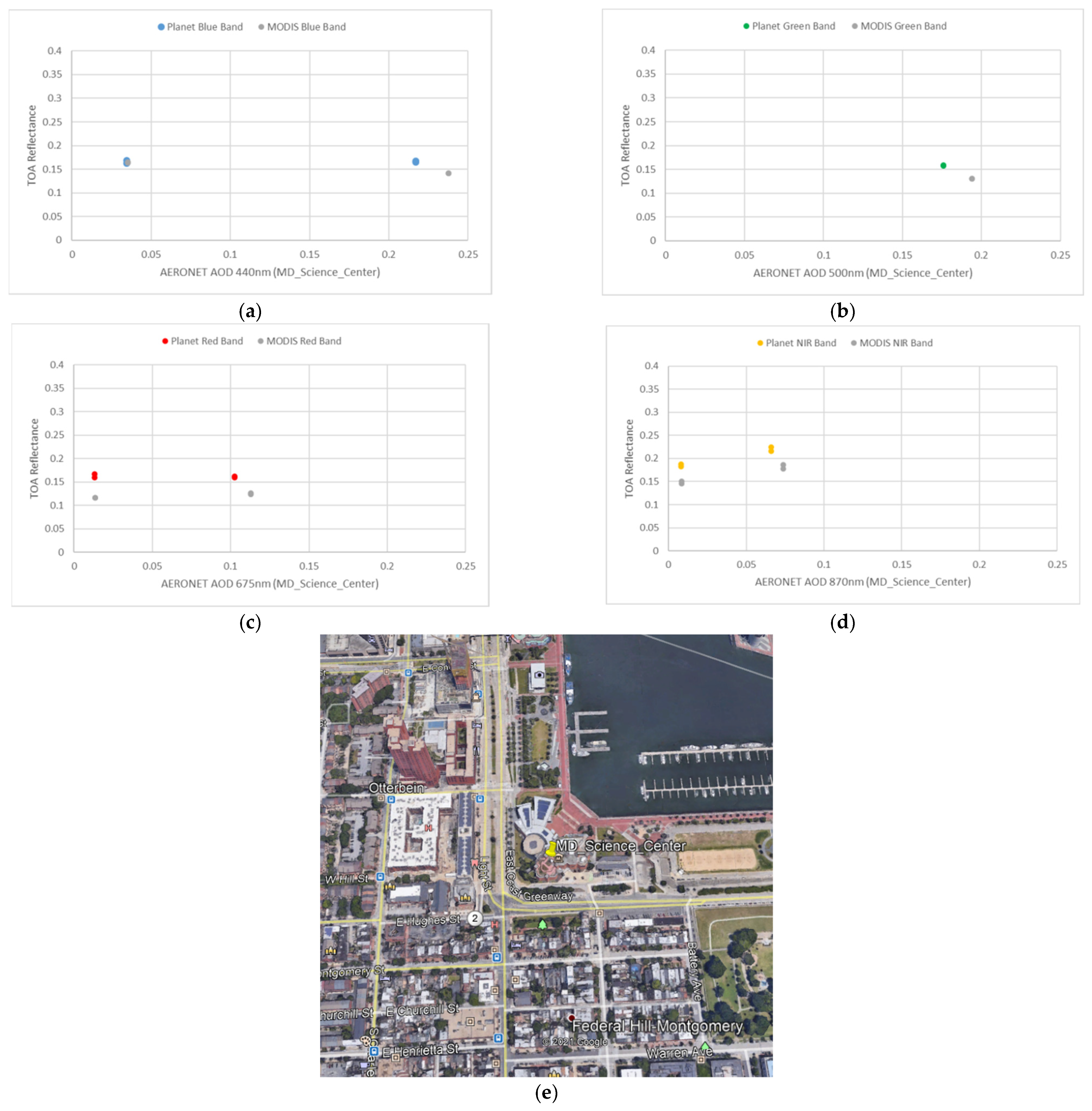
Figure A9.
Data points from Figure 6 isolated for the MD_Science_Center AERONET site. Data points from the 5 × 5 and 10 × 10 pixel average plots are combined. Lower AOD values are from 3/22/2017 and higher AOD values are from 7/14/2018. Plots are separated by (a) blue band; (b) green band; (c) red band; (d) NIR band. No AERONET data was available for the 500 nm band on 3/22/2017 (b), so only values from 7/14/2018 are plotted for the green band. PlanetScope values are in color and MODIS values are in grey. The image in (e) shows a screenshot of the AERONET site location in Google Earth.

References
- Valinia, A.; Burt, J.; Pham, T.; Ganel, O. The role of smallsats in scientific exploration and commercialization of space. In Proceedings of the SPIE Defense & Commercial Sensing, Baltimore, MD, USA, 4–18 April 2019; p. 72. [Google Scholar] [CrossRef] [Green Version]
- Wekerle, T.; Filho, J.B.P.; da Costa, L.E.V.L.; Trabasso, L.G. Status and trends of smallsats and their launch vehicles—An up-to-date review. J. Aerosp. Technol. Manag. 2017, 9, 269–286. [Google Scholar] [CrossRef]
- Martin, L.K.; Jones, W.H.; Shiroma, W.A. Small-satellite projects offer big rewards. IEEE Potentials 2014, 33, 24–30. [Google Scholar] [CrossRef]
- The CubeSat Program, Cal Poly SLO. CubeSat Design Specification Rev. 13. 2014. Available online: https://static1.squarespace.com/static/5418c831e4b0fa4ecac1bacd/t/56e9b62337013b6c063a655a/1458157095454/cds_rev13_final2.pdf (accessed on 29 September 2020).
- Laufer, R.; Pelton, J.N. The Smallest Classes of Small Satellites Including Femtosats, Picosats, Nanosats, and CubeSats. In Handbook of Small Satellites; Pelton, J., Ed.; Springer: Cham, Switzerland, 2019. [Google Scholar] [CrossRef]
- Martin, S. Modern Small Satellites—Changing the Economics of Space. Proc. IEEE 2018, 106, 343–361. [Google Scholar] [CrossRef]
- NASA.gov. The Emerging Commercial Marketplace in Low-Earth Orbit. Available online: https://www.nasa.gov/mission_pages/station/research/news/b4h-3rd/ev-emerging-commercial-market-in-leo (accessed on 29 September 2020).
- Nanosats.eu. Nanosatellite Launches by Organisations. Available online: https://www.nanosats.eu/img/fig/Nanosats_years_organisations_2020-04-20.svg (accessed on 29 September 2020).
- Planet.com. Available online: https://www.planet.com/company (accessed on 29 September 2020).
- Salomonson, V.V.; Barnes, W.L.; Maymon, P.W.; Montgomery, H.E.; Ostrow, H. MODIS—Advanced Facility Instrument for Studies of the Earth as a System. IEEE Trans. Geosci. Remote Sens. 1989, 27, 145–153. [Google Scholar] [CrossRef]
- Houborg, R.; McCabe, M.F. A Cubesat enabled Spatio-Temporal Enhancement Method (CESTEM) utilizing Planet, Landsat and MODIS data. Remote Sens. Environ. 2018, 209, 211–226. [Google Scholar] [CrossRef]
- USGS.gov. USGS EROS Archive-Sentinel-2-Comparison of Sentinel-2 and Landsat. Available online: https://www.usgs.gov/centers/eros/science/usgs-eros-archive-sentinel-2-comparison-sentinel-2-and-landsat?qt-science_center_objects=0#qt-science_center_objects (accessed on 29 September 2020).
- ESA.int. ESA–NASA Collaboration Fosters Comparable Land Imagery. 2013. Available online: https://www.esa.int/Applications/Observing_the_Earth/Copernicus/ESA_NASA_collaboration_fosters_comparable_land_imagery (accessed on 29 September 2020).
- Claverie, M.; Ju, J.; Masek, J.G.; Dungan, J.L.; Vermote, E.F.; Roger, J.C.; Skakun, S.V.; Justice, C. The Harmonized Landsat and Sentinel-2 surface reflectance data set. Remote Sens. Environ. 2018, 219, 145–161. [Google Scholar] [CrossRef]
- Planet.com, 2021. Planet Imagery Product Specifications February. 2021. Available online: https://assets.planet.com/docs/Planet_Combined_Imagery_Product_Specs_letter_screen.pdf (accessed on 6 April 2021).
- EOportal.org. Dove-1 and Dove-2 Nanosatellites. Available online: https://directory.eoportal.org/web/eoportal/satellite-missions/content/-/article/dove (accessed on 29 September 2020).
- Safyan, M. Planet To Launch Record-Breaking 88 Satellites. 2017. Available online: https://www.planet.com/pulse/record-breaking-88-satellites/ (accessed on 29 September 2020).
- The White House, 2016. Harnessing the Small Satellite Revolution. 2016. Available online: https://obamawhitehouse.archives.gov/the-press-office/2016/10/21/harnessing-small-satellite-revolution-promote-innovation-and (accessed on 8 October 2020).
- Earthdata.nasa.gov. Commercial Smallsat Data Acquisition Program. Available online: https://earthdata.nasa.gov/esds/csdap (accessed on 6 April 2021).
- NASA Earth Science Division. Commercial SmallSat Data Acquisition Program Pilot Evaluation Report. 2020. Available online: https://cdn.earthdata.nasa.gov/conduit/upload/14180/CSDAPEvaluationReport_Apr20.pdf (accessed on 8 October 2020).
- Planet.com/pulse. Available online: https://www.planet.com/pulse/ (accessed on 8 October 2020).
- Ephemerides.planet-labs.com. Monthly Planet Satellite Operational Report. 2020. Available online: https://ephemerides.planet-labs.com/operational_status.txt (accessed on 8 October 2020).
- Planet.com. Planet Imagery Product Specification: Planetscope & Rapideye. 2016. Available online: https://www.harrisgeospatial.com/Portals/0/pdfs/PlanetScope-RapidEye-Spec-Sheet.pdf (accessed on 29 September 2020).
- Planet.com, 2015. Planet Labs Specifications: Spacecraft Operations & Ground Systems. Available online: http://content.satimagingcorp.com.s3.amazonaws.com/media/pdf/Dove-PDF-Download#:~:text=Planet%20Labs%20satellites%20are%20designed,operational%20lifetime%20of%203%20years (accessed on 30 September 2020).
- Safyan, M. Liftoff! 20 Next-Generation Dove Satellites Launch On ISRO’s PSLV. 2019. Available online: https://www.planet.com/pulse/liftoff-20-next-generation-dove-satellites-launch-on-isros-pslv/ (accessed on 29 September 2020).
- Doshi, S. Introducing Next-Generation PlanetScope Imagery. 2019. Available online: https://www.planet.com/pulse/introducing-next-generation-planetscope-monitoring/ (accessed on 29 September 2020).
- Breunig, F.M.; Galvão, L.S.; Dalagnol, R.; Dauve, C.E.; Parraga, A.; Santi, A.L.; Della Flora, D.P.; Chen, S. Delineation of management zones in agricultural fields using cover–crop biomass estimates from PlanetScope data. Int. J. Appl. Earth Obs. Geoinf. 2020, 85, 102004. [Google Scholar] [CrossRef]
- Planet News. Planet Announces More Spectral Bands, 50 Cm Resolution, Global Analytics, and Change Detection. 2019. Available online: https://www.planet.com/pulse/more-spectral-bands-50cm-global-analytics-change-detection/ (accessed on 29 September 2020).
- Wang, J.; Yang, D.; Detto, M.; Nelson, B.W.; Chen, M.; Guan, K.; Wu, S.; Yan, Z.; Wu, J. Multi-scale integration of satellite remote sensing improves characterization of dry-season green-up in an Amazon tropical evergreen forest. Remote Sens. Environ. 2020, 246, 111865. [Google Scholar] [CrossRef]
- Houborg, R.; McCabe, M.F. Daily retrieval of NDVI and LAI at 3 m resolution via the fusion of CubeSat, Landsat, and MODIS data. Remote Sens. 2018, 10, 890. [Google Scholar] [CrossRef] [Green Version]
- Leach, N.; Coops, N.C.; Obrknezev, N. Normalization method for multi-sensor high spatial and temporal resolution satellite imagery with radiometric inconsistencies. Comput. Electron. Agric. 2019, 164, 104893. [Google Scholar] [CrossRef]
- Xu, H.; Zhang, L.; Huang, W.; Xu, W.; Si, X.; Chen, H.; Li, X.; Song, Q. Onboard absolute radiometric calibration and validation of the satellite calibration spectrometer on HY-1C. Opt. Express 2020, 28, 30015–30034. [Google Scholar] [CrossRef] [PubMed]
- Gascon, F.; Bouzinac, C.; Thépaut, O.; Jung, M.; Francesconi, B.; Louis, J.; Lonjou, V.; Lafrance, B.; Massera, S.; Glaudel-Vacaresse, A.; et al. Copernicus Sentinel-2A Calibration and Products Validation Status. Remote Sens. 2017, 9, 584. [Google Scholar] [CrossRef] [Green Version]
- Helder, D.; Anderson, C.; Beckett, K.; Houborg, R.; Zuleta, I.; Boccia, V.; Clerc, S.; Kuester, M.; Markham, B.; Paunutti, M. Observations and Recommendations for Coordinated Calibration Activities of Government and Commercial Optical Satellite Systems. Remote Sens. 2020, 12, 2468. [Google Scholar] [CrossRef]
- Aguilera, M.A.Z. Classication of Land-Cover through Machine Learning Algorithms for Fusion of Sentinel-2a and Planetscope Imagery. In Proceedings of the IEEE Latin American GRSS & ISPRS Remote Sensing Conference (LAGIRS), Santiago, Chile, 22–27 March 2020; pp. 246–253. [Google Scholar] [CrossRef]
- Kaplan, G. Assessing the effectiveness of PlanetScope synthesized panchromatic bands for spatial enhancement of Sentinel-2 data. J. Appl. Remote Sens. 2020, 14, 036504. [Google Scholar] [CrossRef]
- Li, Z.; Zhang, H.K.; Roy, D.P.; Yan, L.; Huang, H. Sharpening the Sentinel-2 10 and 20 m bands to planetscope-0 3 m resolution. Remote Sens. 2020, 12, 2406. [Google Scholar] [CrossRef]
- Planet.com. Planet Imagery Product Specifications January. 2018. Available online: https://www.planet.com/products/satellite-imagery/files/Planet_Combined_Imagery_Product_Specs_December2017.pdf (accessed on 29 September 2020).
- Jumpasut, A. Celebrate The Apollo 11 Moon Landing with These Stellar Moon Shots. 2019. Available online: https://www.planet.com/pulse/celebrate-the-apollo-11-moon-landing-with-these-stellar-moon-shots/ (accessed on 29 September 2020).
- Konidaris, N.; Krantz, W.; Warga, J. Pre-launch Calibration of the Planet PlanetScope Constellation. 2016. Available online: https://calval.cr.usgs.gov/apps/sites/default/files/jacie/JACIE-Presentation-Pre-launch-Calibration-of-the-Planet-Labs-PlanetScope-Constellation-1.pdf (accessed on 13 June 2021).
- Jumpasut, A.; Fukuzato, A.; Greenberg, J.; Wilson, N.; Lunar Radiometric Calibration on Planet Dove Satellites. Conference on Characterization and Radiometric Calibration for Remote Sensing (CALCON). 2017. Available online: https://digitalcommons.usu.edu/calcon/CALCON2017/All2017Content/27/ (accessed on 13 June 2021).
- Jumpasut, A.; Fukuzato, A.; Zuleta, I.; Using the Moon as a Calibration Source for a Fleet of Satellites. Conference on Characterization and Radiometric Calibration for Remote Sensing (CALCON). 2018. Available online: https://digitalcommons.usu.edu/calcon/CALCON2018/all2018content/20/ (accessed on 13 June 2021).
- Wilson, N.; Greenberg, J.; Jumpasut, A.; Collison, A.; Weichelt, H. Absolute Radiometric Calibration of Planet Dove Satellites, Flocks 2p & 2e 13. 2017. Available online: https://support.planet.com/hc/en-us/articles/360012629353-Absolute-Radiometric-Calibration-of-Planet-Dove-Satellites-Flocks-2p-2e (accessed on 8 October 2020).
- Liu, Y.; Ma, L.; Wang, N.; Qian, Y.; Qiu, S.; Li, C.; Tang, L. Vicarious radiometric calibration/validation of Landsat-8 operational land imager using a ground reflected radiance-based approach with Baotou site in China. J. Appl. Remote Sens. 2017, 11, 044004. [Google Scholar] [CrossRef]
- Townshed, J.R.G.; Justice, C.O.; Groney, C.; McManus, J. The Impact of Misregistration on Change Detection. IEEE Trans. Geosci. Remote Sens. 1992, 30, 1054–1060. [Google Scholar] [CrossRef] [Green Version]
- Cooley, S.W.; Smith, L.C.; Stepan, L.; Mascaro, J. Tracking dynamic northern surface water changes with high-frequency planet CubeSat imagery. Remote Sens. 2017, 9, 1306. [Google Scholar] [CrossRef] [Green Version]
- Cheng, Y.; Vrieling, A.; Fava, F.; Meroni, M.; Marshall, M.; Gachoki, S. Phenology of short vegetation cycles in a Kenyan rangeland from PlanetScope and Sentinel-2. Remote Sens. Environ. 2020, 248, 112004. [Google Scholar] [CrossRef]
- Pun, V.C.; Kazemiparkouhi, F.; Manjourides, J.; Suh, H.H. Long-Term PM2.5 Exposure and Respiratory, Cancer, and Cardiovascular Mortality in Older US Adults. Am. J. Epidemiol. 2017, 186, 961–969. [Google Scholar] [CrossRef]
- West, J.J.; Cohen, A.; Dentener, F.; Brunekreef, B.; Zhu, T.; Armstrong, B.; Bell, M.L.; Brauer, M.; Carmichael, G.; Costa, D.L.; et al. What We Breathe Impacts Our Health: Improving Understanding of the Link between Air Pollution and Health. Environ. Sci. Technol. 2016, 50, 4895–4904. [Google Scholar] [CrossRef] [PubMed]
- Christopher, S.; Gupta, P. Global distribution of column satellite aerosol optical depth to surface PM2.5 relationships. Remote Sens. 2020, 12, 1985. [Google Scholar] [CrossRef]
- Hoff, R.; Christopher, S. Remote Sensing of Particulate Pollution from Space: Have We Reached the Promised Land? J. Air Waste Manag. Assoc. 2009, 59, 645–675. [Google Scholar] [CrossRef] [PubMed]
- Kaufman, Y.J.; Tanré, D.; Bouche, O. A satellite view of aerosols in the climate system. Nature 2002, 419, 215–223. [Google Scholar] [CrossRef]
- Li, J.; Carlson, B.E.; Lacis, A.A. How well do satellite AOD observations represent the spatial and temporal variability of PM2.5 concentration for the United States? Atmos. Environ. 2015, 102, 260–273. [Google Scholar] [CrossRef]
- Levy, R.C.; Mattoo, S.; Munchak, L.A.; Remer, L.A.; Sayer, A.M.; Patadia, F.; Hsu, N.C. The Collection 6 MODIS aerosol products over land and ocean. Atmos. Meas. Tech. 2013, 6, 2989–3034. [Google Scholar] [CrossRef] [Green Version]
- Wang, J.; Christopher, S.A. Intercomparison between satellite-derived aerosol optical thickness and PM2.5 mass: Implications for air quality studies. Geophys. Res. Lett. 2003, 30, 2–5. [Google Scholar] [CrossRef]
- Zhang, H.; Hoff, R.M.; Engel-Cox, J.A. The relation between moderate resolution imaging spectroradiometer (MODIS) aerosol optical depth and PM2.5 over the United States: A geographical comparison by U.S. Environmental Protection Agency regions. J. Air Waste Manag. Assoc. 2009, 59, 1358–1369. [Google Scholar] [CrossRef] [Green Version]
- Lee, H.J.; Liu, Y.; Coull, B.A.; Schwartz, J.; Koutrakis, P. A novel calibration approach of MODIS AOD data to predict PM2.5 concentrations. Atmos. Chem. Phys. 2011, 11, 7991–8002. [Google Scholar] [CrossRef] [Green Version]
- van Donkelaar, A.; Martin, R.V.; Park, R.J. Estimating ground-level PM2.5 using aerosol optical depth determined from satellite remote sensing. J. Geophys. Res. Atmos. 2006, 111. [Google Scholar] [CrossRef]
- Paciorek, C.J.; Liu, Y. Limitations of remotely sensed aerosol as a spatial proxy for fine particulate matter. Environ. Health Perspect. 2009, 117, 904–909. [Google Scholar] [CrossRef] [Green Version]
- Xiao, Q.; Wang, Y.; Chang, H.H.; Meng, X.; Geng, G.; Lyapustin, A.; Liu, Y. Full-coverage high-resolution daily PM2.5 estimation using MAIAC AOD in the Yangtze River Delta of China. Remote Sens. Environ. 2017, 199, 437–446. [Google Scholar] [CrossRef]
- He, Q.; Huang, B. Satellite-based high-resolution PM2.5 estimation over the Beijing-Tianjin-Hebei region of China using an improved geographically and temporally weighted regression model. Environ. Pollut. 2018, 236, 1027–1037. [Google Scholar] [CrossRef]
- Remer, L.A.; Mattoo, S.; Levy, R.C.; Munchak, L.A. MODIS 3 km aerosol product: Algorithm and global perspective. Atmos. Meas. Tech. 2013, 6, 1829–1844. [Google Scholar] [CrossRef] [Green Version]
- Lyapustin, A.; Wang, Y.; Korkin, S.; Huang, D. MODIS Collection 6 MAIAC Algorithm. Atmos. Meas. Tech. Discuss. 2018, 11, 5741–5765. [Google Scholar] [CrossRef] [Green Version]
- Zhang, X.; Chu, Y.; Wang, Y.; Zhang, K. Predicting daily PM2.5 concentrations in Texas using high-resolution satellite aerosol optical depth. Sci. Total Environ. 2018, 631–632, 904–911. [Google Scholar] [CrossRef] [PubMed]
- Wei, J.; Sun, L.; Peng, Y.; Wang, L.; Zhang, Z.; Bilal, M. An Improved High- Spatial-Resolution Aerosol Retrieval Algorithm for MODIS Images Over Land. J. Geophys. Res. Atmos. 2018, 123, 12291–12307. [Google Scholar] [CrossRef]
- Bai, Y.; Wu, L.; Qin, K.; Zhang, Y.; Shen, Y.; Zhou, Y. A geographically and temporally weighted regression model for ground-level PM2.5 estimation from satellite- derived 500 m resolution AOD. Remote Sens. 2016, 8, 262. [Google Scholar] [CrossRef] [Green Version]
- Di, Q.; Amini, H.; Shi, L.; Kloog, I.; Silvern, R.; Kelly, J.; Sabath, M.B.; Choirat, C.; Koutrakis, P.; Lyapustin, A. An ensemble-based model of PM2.5 concentration across the contiguous United States with high spatiotemporal resolution. Environ. Int. 2019, 130, 104909. [Google Scholar] [CrossRef]
- Xie, Y.; Wang, Y.; Bilal, M.; Dong, W. Mapping daily PM2.5 at 500m resolution over Beijing with improved hazy day performance. Sci. Total Environ. 2019, 659, 410–418. [Google Scholar] [CrossRef]
- Yao, F.; Wu, J.; Li, W.; Peng, J. Estimating daily PM2.5 concentrations in Beijing using 750-M VIIRS IP AOD retrievals and a nested spatiotemporal statistical model. Remote Sens. 2019, 11, 841. [Google Scholar] [CrossRef] [Green Version]
- Kloog, I.; Chudnovsky, A.; Just, A.; Nordio, F.; Koutrakis, P.; Coull, B.; Lyapustin, A.; Wang, Y.; Schwartz, J. A new hybrid spatio-temporal model for estimating daily multi-year PM2.5 concentrations across northeastern USA using high resolution aerosol optical depth data. Atmos. Environ. 2014, 95, 581–590. [Google Scholar] [CrossRef] [Green Version]
- Zhang, T.; Zhu, Z.; Gong, W.; Zhu, Z.; Sun, K.; Wang, L.; Huang, Y.; Mao, F.; Shen, H.; Li, Z. Estimation of ultrahigh resolution PM2.5 concentrations in urban areas using 160m Gaofen-1 AOD retrievals. Remote Sens. Environ. 2018, 216, 91–104. [Google Scholar] [CrossRef]
- Zheng, T.; Bergin, M.; Hu, S.; Miller, J.; Carlson, D. Estimating ground-level PM2.5 using micro-satellite images by a convolutional neural network and random forest approach. Atmos. Environ. 2020, 230, 117451. [Google Scholar] [CrossRef]
- Shen, H.; Li, T.; Yuan, Q.; Zhang, L. Estimating Regional Ground-Level PM2.5 Directly from Satellite Top-Of-Atmosphere Reflectance Using Deep Belief Networks. J. Geophys. Res. Atmos. 2018, 123, 875–13886. [Google Scholar] [CrossRef] [Green Version]
- Planet Team. Planet Application Program Interface: In Space for Life on Earth. San Francisco, CA. Available online: https://api.planet.com (accessed on 28 October 2020).
- Holben, B.N.; Eck, T.F.; Slutsker, I.; Tanré, D.; Buis, J.P.; Setzer, A.; Vermote, E.; Reagan, J.A.; Kaufman, Y.J.; Nakajima, T. AERONET—A Federated Instrument Network and Data Archive for Aerosol Characterization. Remote Sens. Environ. 1998, 66, 1–16. [Google Scholar] [CrossRef]
- Smiley, B. The absolute and relative geolocation accuracies of QB02 and WV01. In Proceedings of the American Society for Photogrammetry and Remote Sensing Annual Conference, Baltimore, MD, USA, 9–13 March 2009; ASPRS: Bethesda, MD, USA, 2009; Volume 2, pp. 787–794. [Google Scholar]
- Fsa.usda.gov. National Agriculture Imagery Program (NAIP) Information Sheet. 2019. Available online: https://www.fsa.usda.gov/Internet/FSA_File/naip_2009_info_final.pdf (accessed on 28 October 2020).
- Suggula, L. What Does the “Ground_Control” Field in the Metadata Signify? 2018. Available online: https://support.planet.com/hc/en-us/articles/360016420313-What-does-the-ground-control-field-in-the-metadata-signify- (accessed on 26 October 2020).
- Schlundt, C.; Kokhanovsky, A.A.; Von Hoyningen-Huene, W.; Dinter, T.; Istomina, L.; Burrows, J.P. Synergetic cloud fraction determination for SCIAMACHY using MERIS. Atmos. Meas. Tech. 2011, 4, 319–337. [Google Scholar] [CrossRef] [Green Version]
- Sun, L.; Wei, J.; Bilal, M.; Tian, X.; Jia, C.; Guo, Y.; Mi, X. Aerosol Optical Depth Retrieval over Bright Areas Using Landsat 8 OLI Images. Remote Sens. 2015, 8, 23. [Google Scholar] [CrossRef] [Green Version]
- Chow, J.; Engelbrecht, J.; Watson, J.; Wilson, W.; Grank, N.; Zhu, T. Designing monitoring networks to represent outdoor human exposure. Chemosphere 2002, 49, 961–978. [Google Scholar] [CrossRef]
Figure 1.
Point locations of the EPA AQS PM2.5 and AERONET monitors utilized for this study. Insets zoom into study areas with multiple monitors. All eight U.S. cities considered regions of interest for this study are noted in the figure.
Figure 1.
Point locations of the EPA AQS PM2.5 and AERONET monitors utilized for this study. Insets zoom into study areas with multiple monitors. All eight U.S. cities considered regions of interest for this study are noted in the figure.

Figure 2.
Schematic illustrating the 5 × 5 and 10 × 10 pixel size averages utilized for the TOA reflectance comparison between PlanetScope and MODIS. The inner boxes represent the 5 × 5 pixel average, whereas the outer boxes represent the 10 × 10 pixel averages (MODIS to the left and PlanetScope to the right). The difference in size between the MODIS (left) and PlanetScope (right) boxes are not to scale.

Figure 3.
Comparison of results for (a) a clear day (1/3/2019); (b) and a hazy day (8/7/2018) for water pixels sampled over Millerton Lake near Fresno, CA. Results for other land cover types sampled in the Fresno and Los Angeles study areas can be found in Appendix A Figure A1, Figure A2, Figure A3, Figure A4 and Figure A5.

Figure 4.
Comparison of results for (a) a clear day (1/3/2019); (b) and a hazy day (8/7/2018) for agriculture pixels sampled near Fresno, CA. Results for other land cover types sampled in the Fresno and Los Angeles study areas can be found in Appendix A Figure A1, Figure A2, Figure A3, Figure A4 and Figure A5.

Figure 5.
Three hour averaged PM2.5 concentration on the x-axis plotted against (a) blue band TOA reflectance for a 5 × 5 pixel average; (b) blue band TOA reflectance for a 10 × 10 pixel average; (c) green band TOA reflectance for a 5 × 5 pixel average; (d) green band TOA reflectance for a 10 × 10 pixel average; (e) red band TOA reflectance for a 5 × 5 pixel average; (f) red band TOA reflectance for a 10 × 10 pixel average; (g) NIR band TOA reflectance for a 5 × 5 pixel average; (h) NIR band TOA reflectance for a 10 × 10 pixel average on the y-axis; for both PlanetScope and MODIS for all 41 data points. PlanetScope points are in color and MODIS points are grey.


Figure 6.
Data points from Figure 5 isolated for the SPOKANE—AUGUSTA AVE station for (a) the blue band; (b) green band; (c) red band; (d) and NIR band. Low PM2.5 values are from 4/19/2018 and high PM2.5 values are from 8/14/2018.
Figure 6.
Data points from Figure 5 isolated for the SPOKANE—AUGUSTA AVE station for (a) the blue band; (b) green band; (c) red band; (d) and NIR band. Low PM2.5 values are from 4/19/2018 and high PM2.5 values are from 8/14/2018.

Figure 7.
Data points from Figure 5 isolated for the Fresno—Garland and Clovis PM2.5 stations for (a) the blue band; (b) green band; (c) red band; (d) and NIR band. Low PM2.5 values are from 1/3/2019 and high PM2.5 values are from 8/7/2018.
Figure 7.
Data points from Figure 5 isolated for the Fresno—Garland and Clovis PM2.5 stations for (a) the blue band; (b) green band; (c) red band; (d) and NIR band. Low PM2.5 values are from 1/3/2019 and high PM2.5 values are from 8/7/2018.


Figure 8.
Three-hour averaged AOD on the x-axis plotted against (a) blue band TOA reflectance for a 5 × 5 pixel average; (b) blue band TOA reflectance for a 10 × 10 pixel average; (c) green band TOA reflectance for a 5 × 5 pixel average; (d) green band TOA reflectance for a 10 × 10 pixel average; (e) red band TOA reflectance for a 5 × 5 pixel average; (f) red band TOA reflectance for a 10 × 10 pixel average; (g) NIR band TOA reflectance for a 5 × 5 pixel average; (h) NIR band TOA reflectance for a 10 × 10 pixel average on the y-axis; for both PlanetScope and MODIS for all 10 data points. PlanetScope points are in color and MODIS points are grey.


Table 1.
Summary of the differences between the three most recent generations of PlanetScope, adapted from Planet’s Imagery Product Specification document [15]. All sensors collect data at 12-bit radiometric resolution with an approximate ground sampling distance of 3.7 m. The reported revisit time is daily at nadir.
| Characteristic | Dove-Classic (PS2) | Dove-R (PS2.SD) | SuperDove (PSB.SD) |
|---|---|---|---|
| Sensor Description | Four-band frame imager; split-frame visible + NIR filter | Four-band frame imager; butcher-block filter providing blue, green, red and NIR stripes | Eight-band frame imager; butcher block filter providing blue, green, red, red-edge, and NIR stripes |
| Spectral Bands | Blue: 455–515 nm Green: 500–590 nm Red: 590–670 nm NIR: 780–860 nm | Blue: 464–517 nm Green: 547–585 nm Red: 650–682 nm NIR: 846–888 nm | Coastal Blue: 431–452 nm Blue: 465–515 nm Green I: 513–549 nm Green II: 547–583 nm Yellow: 600–620 nm Red: 650–680 nm Red-Edge: 697–713 nm NIR: 845–885 nm |
| Coverage Area of Individual Scene (Approximate) | 24 × 8 km | 24 × 16 km | 32.5 × 19.6 km |
Table 2.
PlanetScope and MODIS data acquired for this study. The first column lists the location and dates of the Dove-Classic (PS2) PlanetScope imagery acquired, with dates ranging from 3/22/2017 to 12/15/2019. The second column lists the MOD02HKM tile overlapping most closely to the acquired Planet data. The third and fourth column list the acquisition time of the respective PlanetScope and MODIS imagery, and the last column lists the approximate temporal offset between the two, which ranged from 2 min at the Baltimore, MD study area on 7/14/2018 to 70 min at the Chicago, IL study area on 7/13/2018.
| Study Area Location & Date | MODIS File Identifier | MODIS Acquisition Time (GMT) | Acquisition Time of Corresponding PlanetScope Scenes (GMT) | Approximate Temporal Offset |
|---|---|---|---|---|
| Baltimore, MD 3/22/2017 | MOD02HKM.A2 017081.1520.061. 2017313214630 | 15:20:00–15:25:00 | 15:09:28–15:09:38 | 11 min |
| Baltimore, MD 7/14/2018 | MOD02HKM.A2 018195.1615.061. 2018196014137 | 16:15:00–16:20:00 | 15:17:32–15:23:50 | 2 min |
| Birmingham, AL 1/10/2019 | MOD02HKM.A201 9010.1550.061.2019 011011549 | 15:50:00–15:55:00 | 16:05:25–16:05:39 | 15 min |
| Birmingham, AL 9/3/2019 | MOD02HKM.A201 9246.1615.061.2019 247011649 | 16:15:00–16:20:00 | 16:07:56–16:07:59 | 8 min |
| Bismarck, ND 8/11/2018 | MOD02HKM.A2 018223.1815.061. 2018224074641 | 18:15:00–18:20:00 | 17:07:07–17:07:11 | 68 min |
| Bismarck, ND 10/30/2018 | MOD02HKM.A2 018303.1815.061. 2018304073558 | 18:15:00–18:20:00 | 17:08:50–17:09:02 | 67 min |
| Chicago, IL 3/22/2018 | MOD02HKM.A201 8081.1625.061.2018 082211719 | 16:25:00–16:30:00 | 16:06:21–16:14:08 | 19 min |
| Chicago, IL 7/13/2018 | MOD02HKM.A201 8194.1710.061.2018 195020513 | 17:10:00–17:15:00 | 16:00:00–16:07:53 | 70 min |
| Fresno, CA 8/7/2018 | MOD02HKM.A2 018219.1845.061. 2018220074514 | 18:45:00–18:50:00 | 18:08:38–18:16:46 | 37 min |
| Fresno, CA 1/3/2019 | MOD02HKM.A2 019003.1900.061. 2019004073319 | 19:00:00–19:05:00 | 18:15:19–18:20:37 | 45 min |
| Los Angeles, CA 8/4/2018 | MOD02HKM.A201 8216.1815.061.2018 217074026 | 18:15:00–18:20:00 | 18:01:40–18:06:21 | 14 min |
| Los Angeles, CA 12/15/2019 | MOD02HKM.A201 9349.1800.061.2019 350071716 | 18:00:00–18:05:00 | 18:14:22–18:37:35 | 14 min |
| Phoenix, AZ 9/7/2017 | MOD02HKM.A2 017250.1830.061. 2017261010116 | 18:30:00–18:35:00 | 17:25:41–18:29:17 | 65 min |
| Phoenix, AZ 10/30/2018 | MOD02HKM.A2 018303.1820.061. 2018304073609 | 18:20:00–18:25:00 | 17:27:21–17:43:42 | 53 min |
| Spokane, WA 4/19/2018 | MOD02HKM.A201 8109.1830.061.2018 110074415 | 18:30:00–18:35:00 | 18:10:55–18:10:59 | 20 min |
| Spokane, WA 8/14/2018 | MOD02HKM.A201 8226.1845.061.2018 227075202 | 18:45:00–18:50:00 | 18:15:20–18:16:44 | 30 min |
Table 3.
Summary of AERONET data utilized for this study where latitude and longitude are given in N-S and E-W coordinates, respectively.
Table 3.
Summary of AERONET data utilized for this study where latitude and longitude are given in N-S and E-W coordinates, respectively.
| AERONET Site Name | Coordinates | Date(s) | Study Area |
|---|---|---|---|
| NEON_SJER | 37.109N, 119.732W | 1/3/2019 | Fresno |
| GSFC | 38.992N, 76.840W | 3/22/2017 & 7/14/2018 | Baltimore |
| MD_Science_Center | 39.281N, 76.612W | 3/22/2017 & 7/14/2018 | Baltimore |
| Sigma_Space_Corp | 38.953N, 76.836W | 3/22/2017 & 7/14/2018 | Baltimore |
| UMBC | 39.255N, 76.709W | 3/22/2017 | Baltimore |
| NEON_SERC | 38.890N, 76.560W | 7/14/2018 | Baltimore |
| SERC | 38.889N, 76.556W | 7/14/2018 | Baltimore |
Table 4.
Bandwidths of the MODIS, PlanetScope and AERONET bands used for comparison.
| Bandwidth (nm) | |||
|---|---|---|---|
| Band Color | MODIS | PlanetScope (PS2) | AERONET |
| Blue | 459–479 | 455–515 | 440 |
| Green | 545–565 | 500–590 | 500 |
| Red | 620–670 | 590–670 | 675 |
| NIR | 841–876 | 780–860 | 870 |
Publisher’s Note: MDPI stays neutral with regard to jurisdictional claims in published maps and institutional affiliations. |
© 2021 by the authors. Licensee MDPI, Basel, Switzerland. This article is an open access article distributed under the terms and conditions of the Creative Commons Attribution (CC BY) license (https://creativecommons.org/licenses/by/4.0/).
Share and Cite
MDPI and ACS Style
le Roux, J.; Christopher, S.; Maskey, M. Exploring the Use of PlanetScope Data for Particulate Matter Air Quality Research. Remote Sens. 2021, 13, 2981. https://0-doi-org.brum.beds.ac.uk/10.3390/rs13152981
AMA Style
le Roux J, Christopher S, Maskey M. Exploring the Use of PlanetScope Data for Particulate Matter Air Quality Research. Remote Sensing. 2021; 13(15):2981. https://0-doi-org.brum.beds.ac.uk/10.3390/rs13152981
Chicago/Turabian Stylele Roux, Jeanné, Sundar Christopher, and Manil Maskey. 2021. "Exploring the Use of PlanetScope Data for Particulate Matter Air Quality Research" Remote Sensing 13, no. 15: 2981. https://0-doi-org.brum.beds.ac.uk/10.3390/rs13152981
Note that from the first issue of 2016, this journal uses article numbers instead of page numbers. See further details here.