
Comparison of Gridded DEMs by Buffering


1
Departamento de Ingeniería Cartográfica, Geodésica y Fotogrametría, Universidad de Jaén, 23071 Jaén, Spain
2
Departamento de Expresión Gráfica, Arquitectónica y en la Ingeniería; Universidad de Granada, 18071 Granda, Spain
*
Author to whom correspondence should be addressed.
Remote Sens. 2021, 13(15), 3002; https://0-doi-org.brum.beds.ac.uk/10.3390/rs13153002
Submission received: 17 June 2021
/
Revised: 23 July 2021
/
Accepted: 28 July 2021
/
Published: 30 July 2021
(This article belongs to the Special Issue Perspectives on Digital Elevation Model Applications)
Abstract
:Comparing two digital elevation models (DEMs), S1 (reference) and S2 (product), in order to get the S2 quality, has usually been performed on sampled points. However, it seems more natural, as we propose, comparing both DEMs using 2.5D surfaces: applying a buffer to S1 (single buffer method, SBM) or to both S1 and S2 (double buffer method, DBM). The SBM and DBM approaches have been used in lines accuracy assessment and, in this paper, we generalize them to a DEM surface, so that more area of the S2 surface (in the case of the SBM), or the area and volume (in the case of the DBM) that are involved, more similarly are S1 and S2. The results obtained show that across both methods, SBM recognizes the presence of outliers and vertical bias while DBM allows a richer and more complex analysis based on voxel intersection. Both methods facilitate creating observed distribution functions that eliminate the need for the hypothesis of normality on discrepancies and allow the application of quality control techniques based on proportions. We consider that the SBM is more suitable when the S1 accuracy is much greater than that of S2 and DBM is preferred when the accuracy of S1 and S2 are approximately equal.
1. Introduction
A Digital Elevation Model (DEM) is a bare earth elevation model representing the surface of the Earth without features like houses, bridges and trees [1], which means elevations of the terrain (bare Earth) void of vegetation and man-made features. DEMs can be produced by various techniques (e.g., LiDAR, aerial photogrammetry and remote sensing, etc.) [2]. The DEMs are the basis for other derived models, such as slopes, orientations (aspect), insolation, drainage networks, visual and watershed analysis, etc., which can be easily derived from them through GIS operations [3]. For all these reasons, they have application in numerous disciplines such as agriculture, biology, geology, climatology, telephony, national defense, etc., where they are used for analysis, modeling and decision-making activities.
Given the importance of DEMs, their positional altimetric accuracy must be known through an evaluation method. In order to evaluate a data set, direct and indirect evaluation methods are referred to [4]. The direct evaluation methods are based on the inspection of the items within the data set, and the indirect evaluation methods on external knowledge or experience [4]. The direct evaluation methods can be classified as internal or external. In the first case, the evaluation uses only the data belonging to the same data set. In the second case, an external and independent data set is required (usually considered as a “reference”). Since the proposed methods fall into the category of direct and external, the review that follows will focus on this scope.
Usually, the external data set is considered as a “reference”, and for this purpose independence and greater accuracy are common requirements. The GNSS (Global Navigation Satellite Systems) techniques (e.g., GPS) are the most widely used to obtain reference data for DEMs quality evaluations [5], but the use of other existing DEMs [6,7,8,9,10,11,12] is also very common [5]. From the perspective of the geometry of the elements that are used for evaluation, the DEMs can be evaluated by using points, transects (linear elements) or surfaces, but almost all of the evaluations are based on considering analysis in one dimension (1D) [5] which means that the planimetry is fixed. The planimetry is assumed to be correct, or that it has been previously corrected. In this way, only the elevation discrepancies are analysed.
The points of high positional accuracy that are used to calculate elevation discrepancies can come from GNSS surveys, but sometimes the use of vertices of an existing geodetic net has been reported [13,14] since these points have an easily identifiable location. On other occasions, data from spatial platforms (e.g., as ICESat in [15]) or from existing databases (e.g., as DTED in [16]) are used. Reference [17] performs the assessment using elevation profiles of roads, paths, tracks, etc., using as reference the profiles obtained from The Global Elevation Data Testing Facility. Finally, it should be indicated that there is a high percentage of cases [5] in which the assessment is performed using other DEMs [6,7,8,9,10,11,12].
Focusing on the most statistical part, and on measures of error or discrepancy, two main avenues are offered in the DEM evaluation processes. On the one hand, there is the consideration of the hypothesis of normality, and on the other hand, the denial of this hypothesis. The first case is the most common, and this model is explicitly proposed by numerous studies (e.g., in [18]). [5] indicate that the vast majority of the cases they analysed (89.17%) use this model. In this case, the use of measures of centrality (mean) and dispersion (standard deviation), as well as the mean square error, is common. However, many authors [6,19,20,21,22,23] indicate that positional errors are not normally distributed, and this situation has increased since the expansion of LiDAR data. In this case, common measures are the median, as a measure of the central tendency, and the median absolute deviation (known as “MAD”) [24,25], as a measure of the dispersion. Another alternative is the direct use of the observed distribution of discrepancies in a free-distribution approach [26].
Another relevant perspective in the evaluation of DEM is that provided by the standards. The standards and methods for the estimation and control of positional accuracy of geospatial data are numerous, e.g., the Engineering Map Accuracy Standards [27], the National Standard for Spatial Data Accuracy [28], the ASPRS Positional accuracy standards for digital geospatial data [29], and others [30,31,32]. Some of these standards offer some particular guidelines in the case of altimetry; however, all of them are based on the use of points to carry out the evaluations. Some of these standards explicitly indicate the typology of points as “well-defined points”. This last aspect is not suitable in the case of DEMs, especially when they are registered as a space tessellation (grid). In references [5] and [33], extensive critical reviews of the positional accuracy assessment methods applied to the case of DEMs are made, and it is noteworthy that the majority approach is based on the use of points, regardless of the standard or method that is applied.
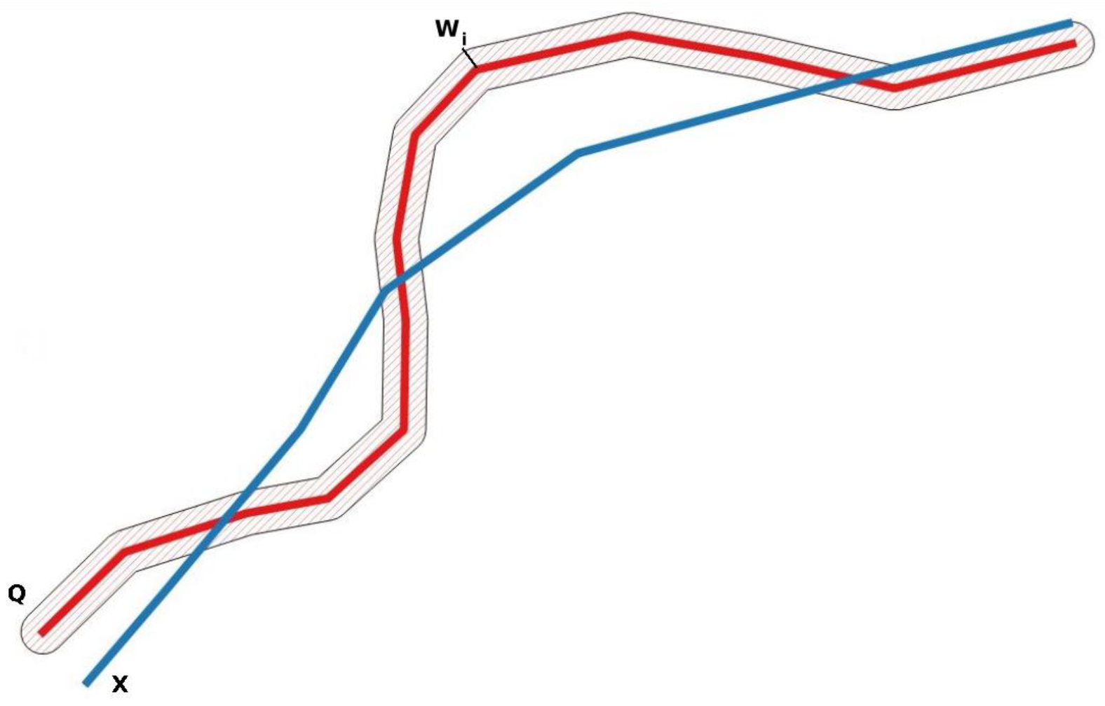
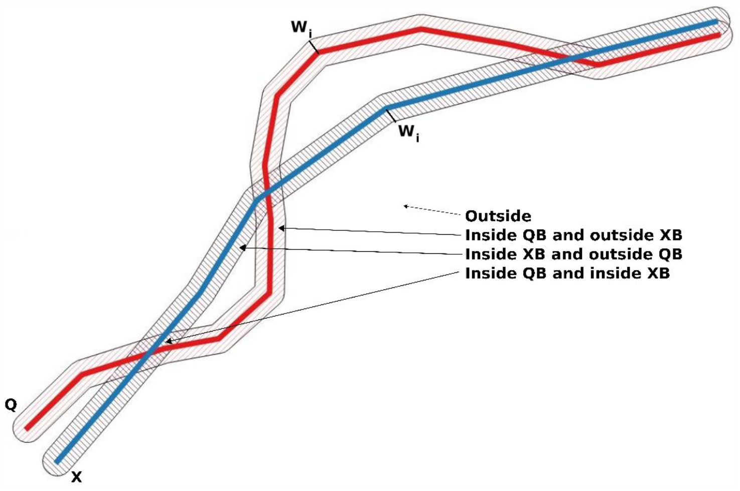
In the case of linear geospatial data, such as communication routes, coastlines or hydrographic networks, in which it is not always possible to find well-defined or homologous points between two representations of the same world feature, specific evaluation methods have been proposed based on buffering, such as the single buffer method (SBM) proposed in [34] (see Figure 1), the double buffer method (DBM) proposed in [35] (see Figure 2), or the “vertex influence method” proposed in [36], and many others. The study of the ability to detect biases, estimate dispersion, detect outliers, etc., in the case of buffer-based methods, has been evidenced in several studies based on synthetic data (e.g., [37,38]) and real data ([39,40,41,42]), etc. Given that these capabilities have been demonstrated in applications on linear elements (e.g., roads, coastlines, etc.), which are more complex than altimetry profiles, we consider that these methods are fully adequate for the case of DEM.
In this work, it is proposed to apply buffer-based methods (simple and double) on gridded DEM data considered as 2.5D surfaces with the aim of comparing the altimetric behavior of both data sets. With this perspective, the disadvantage of not having well-defined points in the case of grid-type DEMs is avoided and, furthermore, it can be applied in the natural context of the reality being analyzed, which is that of the Earth’s surface. Methods based on DEM buffering can be used to compare two sets of DEM data, or a product and a reference that serves for its quality assessment (e.g., quality control or quality estimation).
This document is organized as follows: after this introduction, the next section (2nd) presents the buffer-based methods, their adaptation to the case, and the data sets for the application example. The fourth section develops a discussion and, finally, the main conclusions of the work are included.
2. Methods and Data
The adaptation of the SBM and DBM to the case at hand is presented below. First, an outline of the idea on which the method is based will be presented in its application to the original case of linear elements, and then it will be discussed how to adapt it to the case of DEM surfaces.
2.1. The Single-Buffer Method
Since the SBM was designed for linear elements, for its explanation we will consider two of them here: Q (reference) and X (element to analyze). The SBM consists of generating incremental buffers of semi-width wi around (both sides) of the Q line (denoted by Qwi), and counting the percentage of the line X that is included inside that buffer width [12]. Figure 1 presents a graphical excerpt. The parameter w will take values from approximately zero to the one that allows the total length of X to be included. The method can be applied to a line, as explained, or to a set of homologous paired lines Qj and Xj, obtaining an aggregate result of all of them for each wi. If the percentage of line lengths that is included for each value of w is considered, an observed distribution function is available that defines the phenomenon of interest: the percentage of inclusion of assessed lines versus the buffer widths of the reference lines.
The method described in the previous paragraph is directly transferable to the case of DEMs. First, we will consider two surfaces S1 and S2, such that S1 acts as a reference and S2 as a product. Furthermore, we must assume that the planimetric uncertainty is negligible, in such a way that the buffer can be done directly on the altimetric component. This supposition is a rule for positional accuracy assessments when dealing with DEMs. When the SBM is applied to linear elements, it is not considered whether the inclusion of X in the buffer of Q is made to one side or the other. However, since in this case there is the physical sense that one surface is above or below the other (e.g., S1 on S2), it is interesting to make this distinction (above and below), and also to consider absolute values of discrepancies. In the case of grid-type DEMs, like the one at hand, the SBM application process is very simple, it is enough to calculate the difference between both DEMs (S2-S1) and order the discrepancy (errors) values from smallest to largest obtained, and count the accumulated area.
Considering S1 and S2 has the same rows (m) and columns (n) we denote the homologous cells as S1r,c and S2r,c ( and the height difference of homologous cells as hdr,c = S2r,c − S1r,c:
If is inside the buffered by the semi-width
The percentage of S2 inside the S1 buffered by the semi-width is
In this way we can obtain three curves
- (a)
- one for the evolution of negatives discrepancies (S2 below S1, i.e., ),
- (b)
- also the same for positive discrepancies (S2 above S1, i.e., )
- (c)
- and in absolute value (i.e., ).
The curves thus obtained have the same properties as that generated in the original method for linear elements, in such a way that it can be applied to a DEM or to a set of “patches” (e.g., several zones or patches of a larger DEM).
2.2. The Double-Buffer Method
Continuing with the two linear elements, Q (reference) and X (element to analyze), presented previously, the DBM consists of generating incremental buffers of semi-width wi around (both sides) of the Q and X lines. Figure 2 presents a graphical excerpt. In this case, the proposal by [13] is to count several measures that evolve with wi. Being AX(wi) the area of the buffer over X for the width wi, and AQ(wi) the area of the buffer over Q for the same width, these measurements correspond to the following areas: , , , and, based on them, establish an average displacement and the possibility of counting the number of oscillations. The last determination is linked to the possibility of analyzing the randomness of the lateral displacements of X with respect to Q. The parameter w will take values from approximately zero to that which allows the total length of X and Q to be included in the buffer. The method can be applied to a pair X, Q of lines, as explained, or to a set of lines Qj and Xj, obtaining an aggregate result of all of them for each wi. As a result, a curve with characteristics of the observed distribution function is obtained.
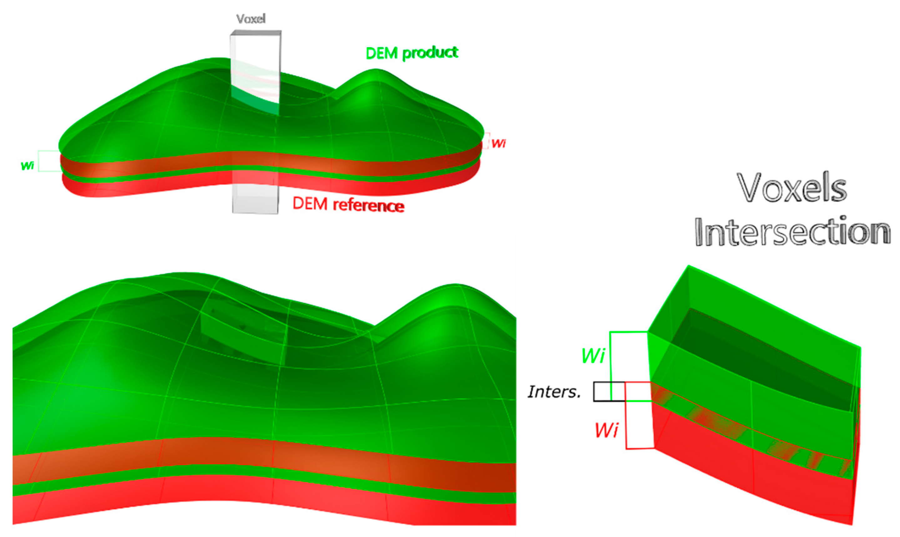
The same assumption as in Section 2.1 has to be considered for the DBM with respect to the planimetric uncertainty component. Furthermore, the method described in the previous paragraph should be slightly adapted for its application to the case of grid-type DEM (Figure 3). Considering that S1 acts as a reference and S2 as a product, we proceed to establish the incremental buffering on the two surfaces. For the analysis with grid-type data, it is convenient to introduce the concept of voxel specified for this context. A voxel is a volume that has as its central section a cell of the grid-type DEM on whose elevation we work, and a height wi on each side (above and below) of that cell. When working with two surfaces S1 and S2 for each position two voxels are considered, one for S1 and another for S2, and we must pay attention to the following situations:
- There is no intersection. There is no intersection between the voxels of the two buffered surfaces. This means that the vertical distance between S1 and S2 exceeds 2 × wi.
- There is an intersection. There is an intersection between the voxels of the two buffered surfaces. This means that the vertical distance between S1 and S2 is less than 2 × wi. If the distance between S1 and S2 is zero, there will be a complete match of the voxels (100% intersection). In this case, for a given wi and a specific position in the DEM, the degree of intersection between the voxels of S1 and S2 can be considered as a fuzzy or probabilistic approximation.
2.3. Data
We apply the SBM and DBM to DEM data obtained in a study area around Allo (Navarra, Spain). The following DEMs data sets are used:
- DEM02. This is a gridded DEM (2 × 2 meter resolution), it was generated in 2017 and its primary data source is an aerial LiDAR survey (RMSEz ≤ 20 cm) (second coverage of the PNOA-LiDAR project https://pnoa.ign.es/estado-del-proyecto-lidar/segunda-cobertura, accessed on 28 July 2021). The informed positional accuracies for the DEM are RMSEXY ≤ 50 cm and RMSEZ-02 ≤ 25 cm. It is considered as the reference in our work: S1.
- DEM05. This is a gridded DEM (5 × 5 meter resolution), it was generated in 2012 and its primary data source is an aerial LiDAR survey (RMSEz ≤ 40 cm) (first coverage of the PNOA-LiDAR project https://pnoa.ign.es/estado-del-proyecto-lidar/primera-cobertura, accessed on 28 July 2021). The informed positional accuracies for the DEM are RMSEXY ≤ 50 cm and RMSEZ-05 ≤ 50 cm. It is considered as the product under analysis in our work: S2.
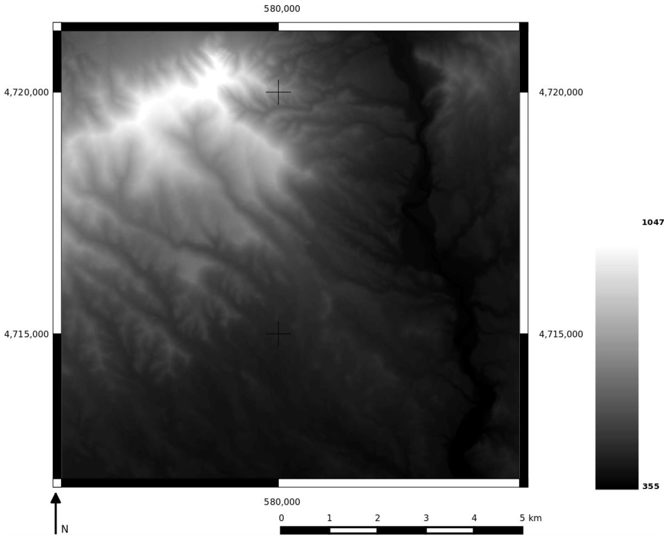
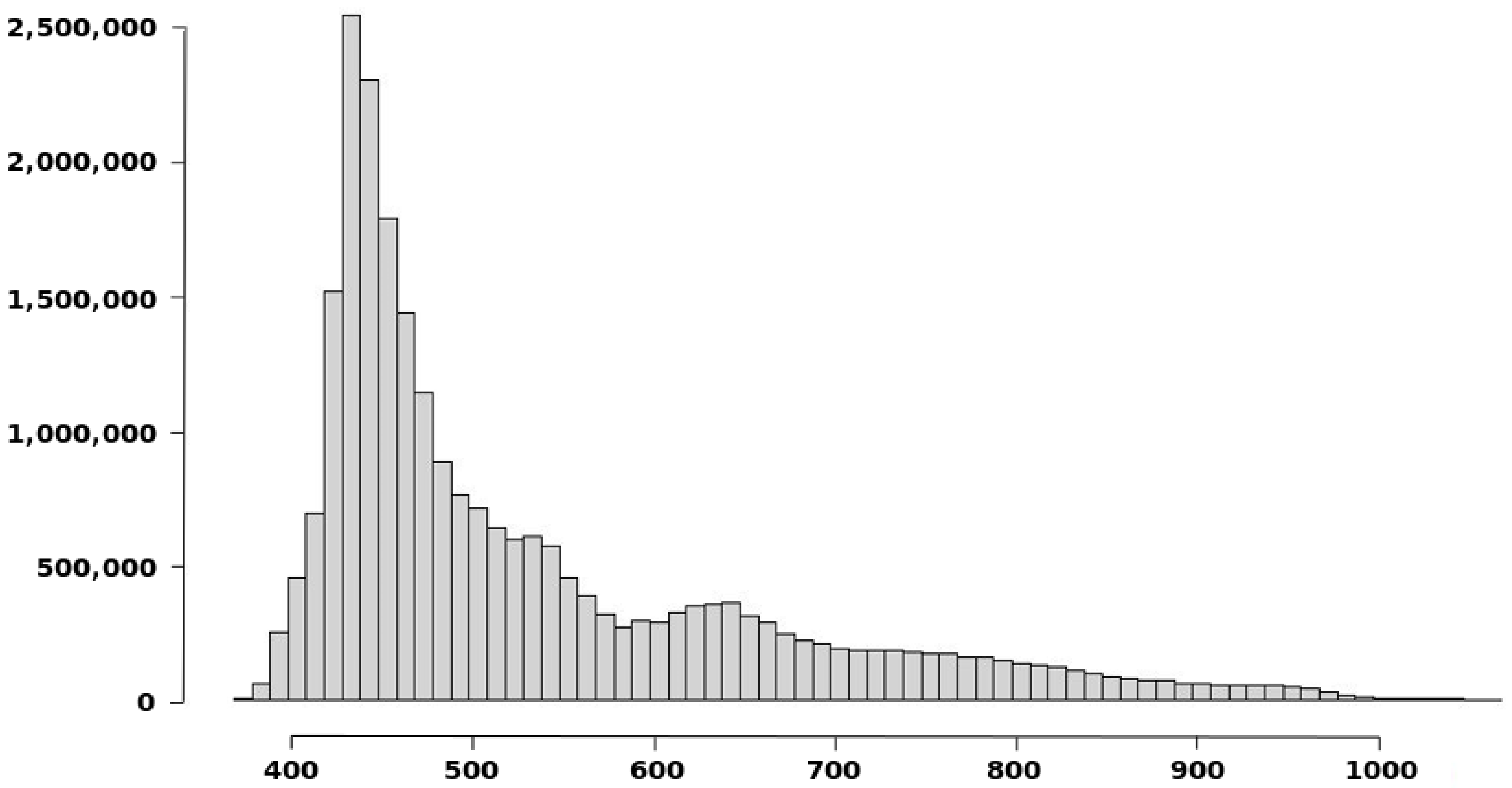
Both DEM data sets come from the Instituto Geográfico Nacional (IGN, Spain, www.igne.es, accessed on 28 July 2021) and are freely available, and have the same spatial reference system ETRS89 UTM Zone 30N with the following coordinates 577,845 m, 4,715,566 m. In relation to the study area, Figure 4 shows a general vision and Figure 5 the corresponding histogram for the elevations. In both figures, the data correspond to the DEM02 data set, (the data corresponding to the DEM05 data set are not presented since visual differences would not be appreciated at this scale of representation). The study area covers 100 km2, and it has a varied relief, but not abrupt, with valleys of different widths, and areas with different degrees of undulation. In order to dispose of some terrain morphological variability, the study area includes a small mountain (Montejurra) and a valley created by the Ega river The elevation is in the interval 354–1047 m, mean value of elevation is 513.66 m and the standard deviation of the elevation is 127.93 m.
To ensure the overlap of the two grids, and not degrade the quality of the reference (DEM02), the MDE05 data set was interpolated with a 2 × 2 mesh step. Following the variance prediction model for the case of bilinear interpolation developed by [43], considering the equality of all the variances of the four positions that intervene in the bilinear interpolation, and the case of a high altimetric correlation, the average variance of the predictor of an altimetric value over any position is equivalent to the variance of the positions involved in the interpolation. In our case, according to the information provided by the metadata, it can be considered to be of the order of 50 cm.
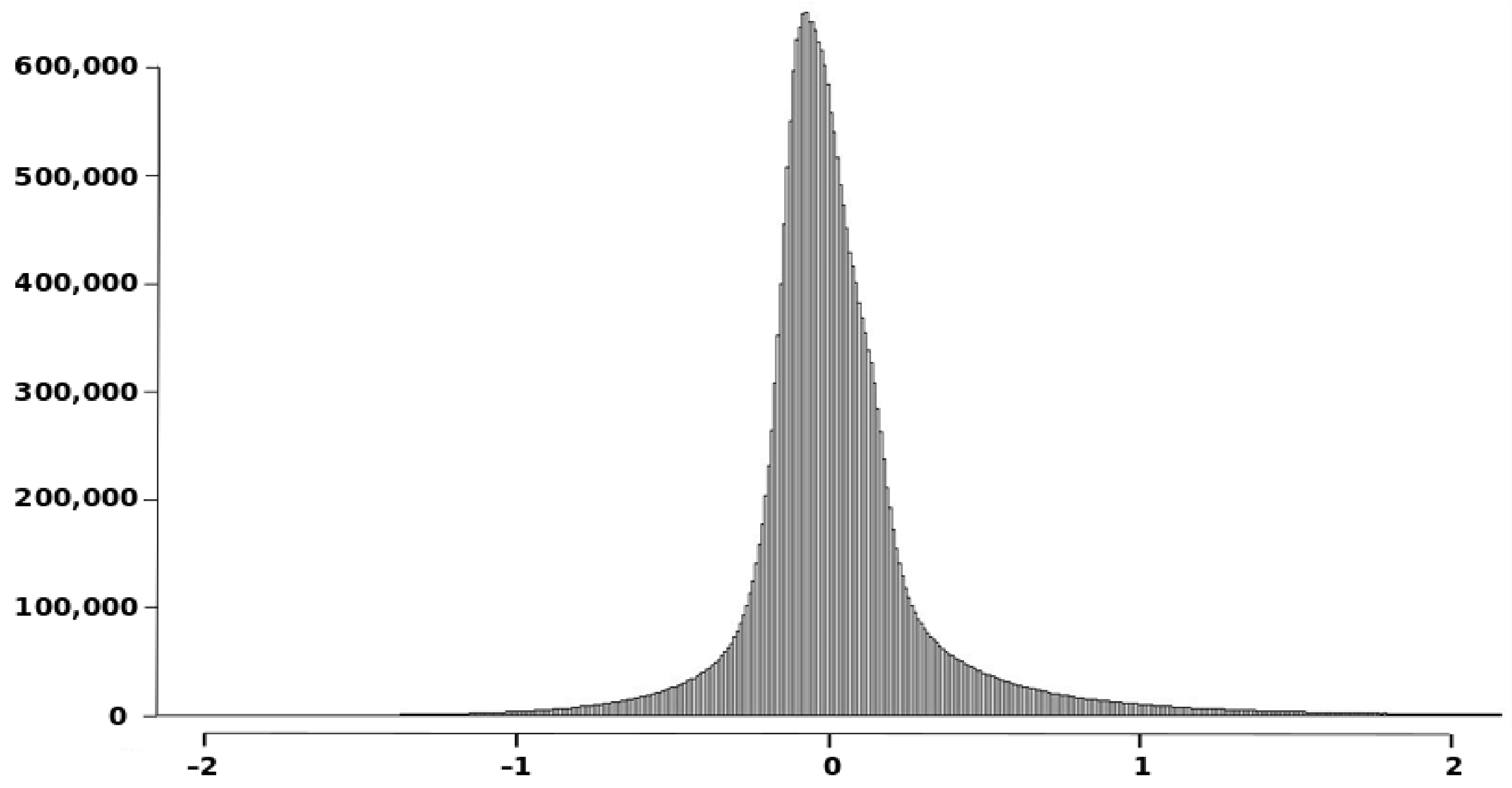
The discrepancies (or vertical errors) between both DEM data sets can be observed in Figure 6 and the histogram in Figure 7, which is presented for the interval [−2, 2] where the majority of values are included. Usually, the values assumed for the discrepancies between a product and a reference must be close to zero, but in this case, it is observed (Figure 6) that discrepancies are in the interval [–55.39, 10.81] m, which means the presence of extreme values (outliers). The position of some of these outliers is highlighted with a red circle in Figure 6. The mean value of the discrepancies is μ = −0.0347 m and the standard deviation σ = 0.6414 m.
3. Results
3.1. The Single-Buffer Method
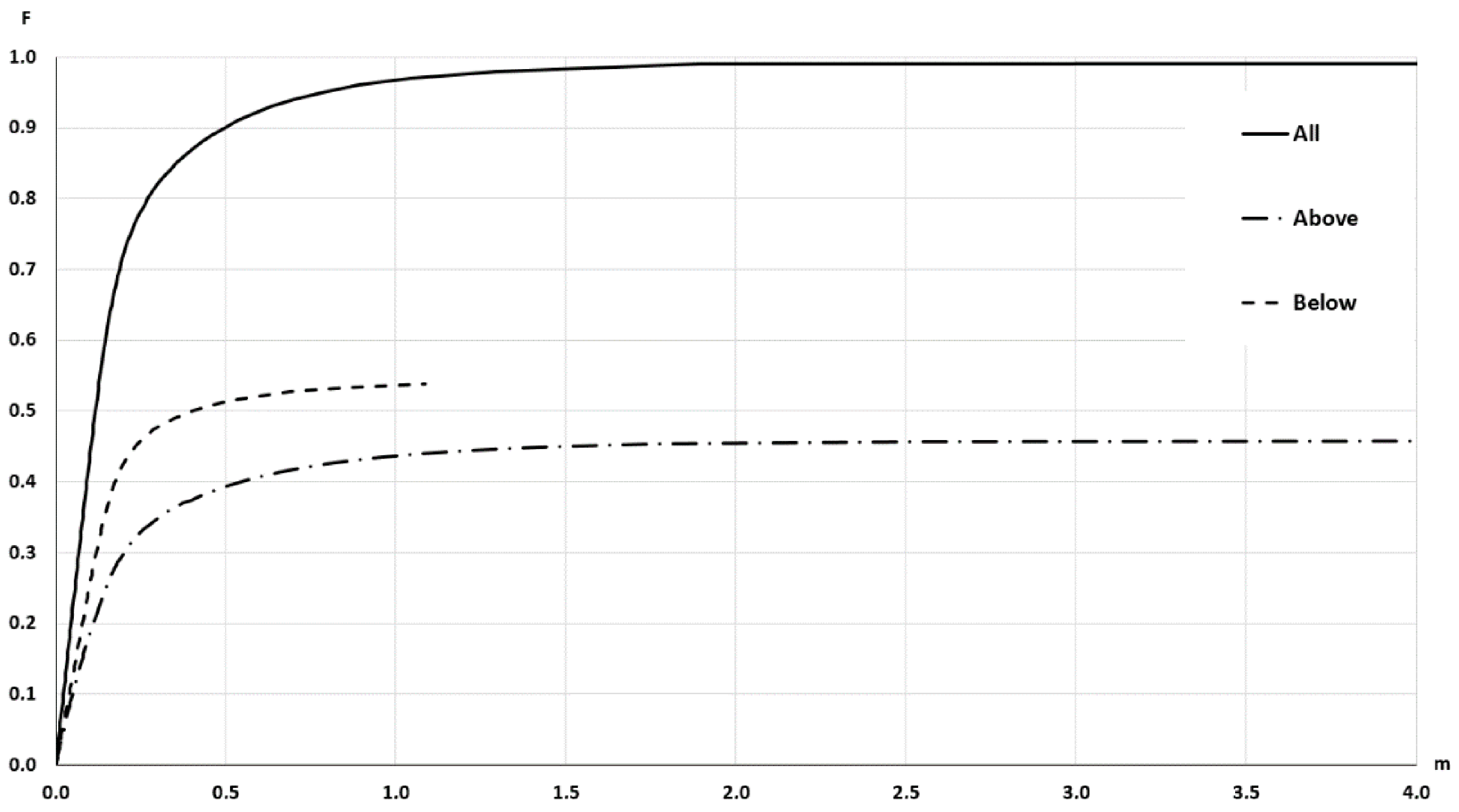
Applying the procedure indicated in Section 2.1, the result shown in Figure 8 can be obtained. This curve has a very long tail until it reaches the extreme value (55.39 m), but to facilitate visual interpretation, only the interval [0, 4] is presented. This curve represents the distribution function of the area of S2 included inside a buffer with wi. S1 is buffered on both sides and results are presented for above, below and the general case (above + below). These curves allow us:
- To recognize the presence of outliers. Outliers are excessively large discrepancies between the S1 and S2 with low presence probabilities and, in general, would correspond to the presence of peaks or wells. This presence would generate the need for a very large value of wi to achieve their inclusion and an asymptotic flattening of the curve close to the value of unity on the vertical axis (100% inclusion). As can be seen in Figure 8, this is the case 99% inclusion is reached approximately for 1.89 m, while there is a long tail, which will extend up to 55.39 m to achieve 100% inclusion. Thus, in the data under analysis, there is the presence of outliers.
- To recognize the presence of vertical bias. The vertical bias, in this case, means that one DEM has an altimetric predominance over the other. In this case, we compare the curves for the cases Above and Below and observe that the below curve is over the above curve. This implies that, in general, S1 is over S2, which means a vertical bias. Here we can remember that the mean value of the discrepancies is μ = –0.0347, the bias is small but in terms of frequencies the difference is in the order of 7.57%, which means an imbalance between the Above and Below cases.To determine the uncertainty, either by establishing a percentile of interest (e.g., 90%) and determining the corresponding distance (≈0.5 m), or by establishing a distance (e.g., d = 1 m) and determining its corresponding percentile (96.5%). The use of a single percentile is fully equivalent to what is proposed in some DEM evaluation methods for non-normal data (e.g., [2,6]). However, the use of a curve such as the one presented in Figure 8 offers much more information and the possibility of using several percentiles for better control of the distribution of discrepancies. In this line, the method proposed by [26] allows the use of several tolerances for the case of non-normal data.
The layout of the curve obtained is totally equivalent to that generated by the SBM on lines, and its interpretation is exactly the same, but substituting percentage of line length by percentage of DEM area, as already indicated. Likewise, it can be applied to a single DEM data set, as in the presented case, or to multiple DEMs data sets or for several patches of a single DEM in an aggregated way. On the other hand, the curve presented in Figure 8 is fully comparable to that used by [26] to apply a method of positional control by points that is based on the application of several tolerances and a multinomial law to take into account different percentages of error cases.
3.2. Double-Buffer Method
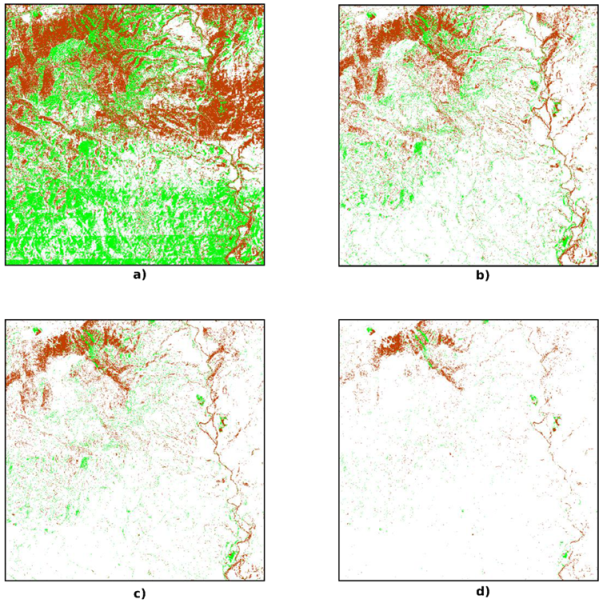
The direct application of the method indicated in Section 2.2 allows obtaining various results, some of which are presented below. In order to understand the process, Figure 9 shows the evolution of areas below (in green), above (in reddish) and within (in white) the buffered surfaces S1 and S2 for w = [0.05, 0.15, 0.25, 0.5]. As is logical, the tendency is that as w increases, the area with white color increases. It is interesting to note that there is no homogeneous distribution of red and yellow colors, which indicates the preponderance of discrepancies (negative and positive) in different areas of the study zone.
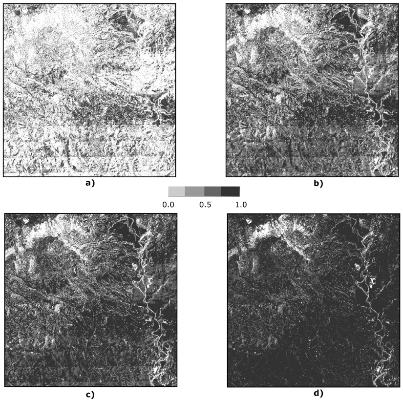
Figure 10 presents a complementary perspective to the previous one. In this case, what is shown is the degree of buffer-overlapping. That is, only for the case of the white areas in Figure 8 above, the degree of buffer-overlapping between S1 and S2 is presented with gray colors ranging from light to dark. Now the trend is that as w increases, there will be a greater level of buffer-overlapping. Figure 10d is the darkest of all as it has the widest buffer width. This level of overlap can be understood as a degree of confidence in the existence of an effective overlap between S1 and S2.
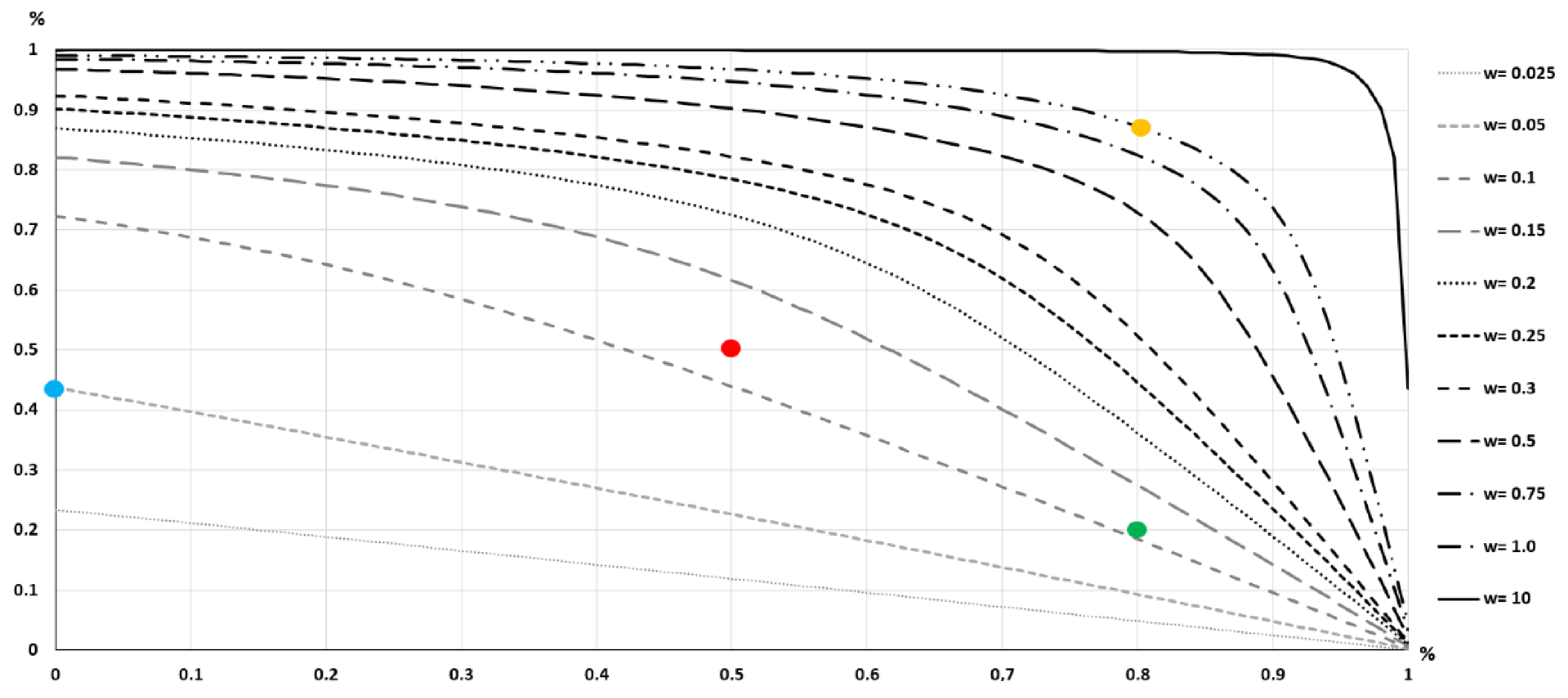
These spatial results can also be expressed by curves, as is shown in Figure 11. Now, let us consider a larger range of semi-width values: wi ∈ [0.025, 0.05, 0.1, 0.15, 0.2, 0.25, 0.3, 0.5, 0.75, 1, 10] m. In Figure 11, the horizontal axis corresponds to the percentage of common intersection between voxels of S1 and S2 (voxel-overlapping), and the vertical axis to the percentage of area of the DEM zone included by each wi and voxel-overlapping value. We can distinguish two groups of curves; first, those that are practically straight lines (corresponding to wi ∈ [0.025, 0.05, 0.1] m, and second, those that are more or less convex curves, corresponding to wi ∈ [0.25, …, 10] m. The curves of the first type intersect the vertical axis on the left by the percentage of the area that wi can include for all percentages of voxel-overlapping. Thus, with wi = 0.05 m only approximately 43% of the area can be covered (blue point). The rest is out of the buffer width capability, so for this buffer width surfaces S1 and S2 have more than 57% of their area outside this analysis.
Convex curves do achieve high values of percentage of area (e.g., 90.1, 96.7, 99.1 for widths of 0.25, 0.5 and 1 m respectively). To understand how this graph works, first let us look at a value of voxel-overlapping (e.g., 80%) and then at the curves corresponding to the wi value of interest (e.g., 0.1 m and 1 m). The cross between the curve corresponding to w = 0.1 m with the vertical for 80% of voxels-overlapping gives ≈18% (green point). This value means that when working with w = 0.1 m there is 18% of the area that has more than 80% of voxel-overlapping. On the other hand, it also indicates that approximately 54% (=72% − 18%) of the area has voxel-overlapping less or equal than 80%. The interpretation is exactly the same for the case of the curve corresponding to w = 1 m. The cross between the curve corresponding to w = 1 m with the vertical for 80% of voxels-overlapping gives ≈88% (yellow point). This value means that when working with w = 1 m there is 88% of the area that has more than 80% of voxel-overlapping. On the other hand, it also indicates that approximately 11% (=99% − 88%) of the area has voxel-overlapping less or equal than 80%. This graph allows us to determine the value of w that would offer a certain percentage of voxel-overlapping affecting a certain percent of the area. For example, if you want at least 50% of the area to have a 50% or more overlap level, we must look at the point (overlap ≥ 50%, area ≥ 50%) (red point). Any curve that passes above this point meets these conditions. In the case of Figure 11, the curve corresponding to wi = 0.15 m is the first one that satisfies this double condition.
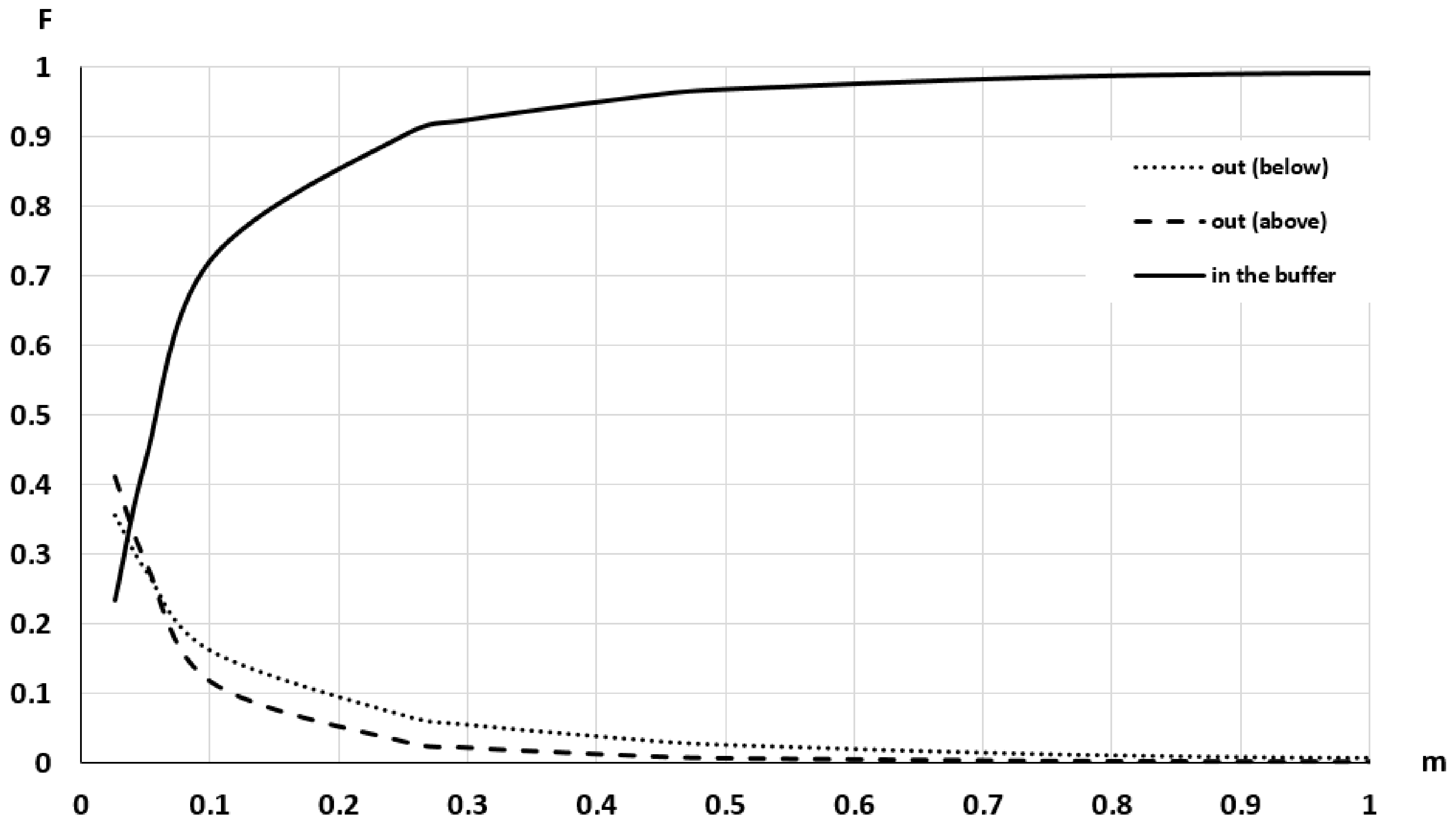
The complex result presented in Figure 11 can be taken to a representation in some way similar to that of Figure 8 corresponding to the SBM. This is presented in Figure 12. In this case, the horizontal axis represents the buffer width w, here it is only presented up to 1 m to appreciate the starting zone in greater detail. The vertical axis represents the percentage of the involved area. The curves labeled as below and above correspond to the red and yellow areas of Figure 9, respectively so that these curves represent the evolution of these areas when increasing wi, and of course, the percentage of the involved area is reduced by increasing wi. If the curve labeled “in the buffer” of Figure 12 is compared with the curve labeled “All” presented in Figure 8, a great similarity is observed, but if it is observed in greater detail (e.g., observe the included area for w = 0.5 m and w = 1 m in both curves), it is concluded that they are not exactly the same, and that the curve corresponding to the DBM is always above the SBM curve. The mean difference between both curves is in the order 11%. This shows that both evaluation methods are very similar, but that they do not perform the same type of measurement.
The results presented for the SBM and DBM methods allow us to conclude that S1 and S2 are very similar but that there are marked differences. For the case of the RMSE composed of the two DEM, according to Section 2.3 (), both in Figure 8 and Figure 12, percentages of areas greater than 90% are obtained. This means that there is a great resemblance. However, quite large values for outliers were detected along with a spatial behavior that shows a clear presence of spatialized bias which is not randomly distributed (see the clustered spatial preponderance of the red and yellow areas in Figure 8). The curves labeled “above” and “below” in Figure 8 and Figure 12 corroborate this situation, and also the predominance of the case “below”. That is, S2 is somewhat sunk with respect to S1.
The curves and figures generated as results are descriptive of the similarity and differences between S2 and S1, but could also be the basis for acceptance/rejection processes if specifications were available. For example, if it had been considered as a specification that for a buffer width w = 3 × RMSE the product under control must have at least 95% of the area within the buffer and that, at least 50% of the population has a voxel-overlap level greater than 50%, Figure 11 would indicate that this condition is fulfilled for S2 with respect to S1.
4. Discussion
Since our greatest interest in this work is the methodological proposal, the discussion will focus on different key aspects that we consider regarding the use of buffer methods:
- Concept. The leap from the application of buffering methods from lines to DEM is quite straightforward and the concepts handled are very similar. The application of the buffer methods to lines entails a certain dimensional change, from 1D to 2D, which in our proposal should have led to a step from 2D to 3D. For simplicity, and because it is more usual to deal with area units than with volume units, the first perspective was developed. The presence of the 3D perspective is included in the application of the DBM when dealing with voxel-overlapping. Of course, the volume could also have been analyzed for the case of the SBM, but in this case, a curve like the one in Figure 8 would be obtained but scaled in units of volume. The use of areas allows the application of these methods also quite directly to the case of other variables such as slope and elevation.
- Algorithms. The application to the case of grid-type DEMs is straightforward, the use of simple map algebra operations allows executing these processes without problem, with agility and for large amounts of data. Working with other DEM data would require coding more complex algorithms.
- Analysis element. In this sense, there is a radical change with respect to the assessment usually applied to DEM, which is based on points (e.g., altimetric error assessments). The analysis based on surfaces seems to us more natural and closer to the reality that we want to analyze. As in the case of application to linear elements, the proposed methods allow them to be applied to a single surface, or to a set of surfaces, regardless of their extension.
- Discrepancies. Since distributional curves are obtained (e.g., those of Figure 8, Figure 11 and Figure 12), more information is available on the behavior of the discrepancies between two DEM data sets. Since the discrepancies do not usually fit a normal distribution, having curves relative to observed distributions allows working with percentiles in a direct way. In the case of wanting to carry out quality control (hypothesis testing), these curves can be used as a basis for control methods based on tolerances (one or more tolerances) (see [26]).
- Analysis capabilities. In relation to the results and possibilities of analysis, the SBM and the DBM are different, as happened in the case of application to linear data and their complementary results, since they present two different perspectives of the same reality. In general, the results of the SBM are easier to interpret than those of the DBM when a partial voxel intersection perspective is adopted on it. In any case, both methods generate curves very similar to observed distribution functions (global or partial). This offers a powerful analysis tool since it visualizes what happens in the entire population or sub-population of interest. Furthermore, the use of these observed distribution functions eliminates the need for the normality hypothesis on discrepancies and allows the application of quality control techniques by means of tolerance(s).
- Applicability of SBM and DBM. We consider that the SBM is more suitable for the case in which the accuracy of S1 is much greater than that of S2, in such a way that it can be considered negligible. In the case of analysis of positional accuracy by points, this circumstance is considered valid when its accuracy is at least three times better. In this case, discrepancies can be considered as errors of S2 in relation to the reference (S1). We consider the DBM to be more suitable for the case where the accuracy of S1 and S2 are approximately equal.
5. Conclusions
This research proposes the use of buffering methods for the comparison of DEMs. Buffer methods have originated in the field of evaluating linear elements, where their use is consolidated, but not widespread. The application of buffering methods to the case of DEMs is a logical consequence since, in principle, they are more suitable for dealing with continuous realities and where it is difficult to find “easily identifiable and well-defined points” as required in the positional accuracy standards (e.g., [5]).
The application of the methods to the case of gridded DEMs is quite straightforward, although it requires some adaptation for the DBM, but, in any case, they are solved with simple map algebra operations. The results of the SBM allow a direct relationship with already developed positional control methods, which are based on control by tolerances applying a multinomial law. Furthermore, the area inclusion curve per buffer width allows conclusions to be drawn about the presence of outliers and biases. The results of the DBM are richer and more complex than those of the SBM since it is played with the degree of intersection of the voxels (voxel overlapping) of the two buffers, which allows a probabilistic interpretation that, in addition, can help to a visual interpretation. This method also makes it possible to analyze the presence of biases. The results of both methods are complementary to the existing ones that are based on parameters (e.g., root mean square error, deviation). In addition, we consider that they present a richer perspective by offering a broader view of what is happening through distributional curves.
The two methods presented here were applied to altimetry, but can also be applied, mutatis mutandis, to the case of slopes and orientations. In this way, it is possible to have a homogeneous approximation to the most used variables of a DEM.
In the future, we plan to develop our method using a wide set of DEMs based on producer specifications to be accomplished and then try several values for wi in order to perform a quality control deciding amongst acceptance or rejection.
Author Contributions
Conceptualization, F.J.A.-L.; methodology, F.J.A.-L.; software, J.F.R.-G.; formal analysis, J.F.R.-G.; investigation, F.J.A.-L. and J.F.R.-G.; resources, F.J.A.-L.; data curation, J.F.R.-G.; writing—review and editing, F.J.A.-L. and J.F.R.-G.; project administration, F.J.A.-L.; funding acquisition, F.J.A.-L. and J.F.R.-G. All authors have read and agreed to the published version of the manuscript.
Funding
This research was partially funded by the research project “Functional Quality in Digital Elevation Models in Engineering” (https://coello.ujaen.es/investigacion/web_giic/funquality4dem/, accessed on 28 July 2021) of the State Research Agency. PID2019-106195RB-I00/AEI/10.13039/501100011033.
Data Availability Statement
DEM02 can be found at https://pnoa.ign.es/estado-del-proyecto-lidar/segunda-cobertura, and DEM05 can be found at https://pnoa.ign.es/estado-del-proyecto-lidar/primera-cobertura (both accessed on 28 July 2021) Their spatial reference system is ETRS89 UTM Zone 30N with the following coordinates 577,845 m, 4,715,566 m.
Conflicts of Interest
The authors declare no conflict of interest.
References
- GISGeography. GIS Dictionary—Geospatial Definition Glossary. 2021. Available online: https://gisgeography.com/gis-dictionary-definition-glossary/#D (accessed on 28 July 2021).
- Maune, D.F. (Ed.) Digital Elevation Model Technologies and Applications: The Dem User’s Manual; American Society for Photogrammetry and Remote Sensing: Bethesda, MD, USA, 2007; ISBN 978-1-57083-082-2. [Google Scholar]
- Felicísimo, M.A. Modelos Digitales Del Terreno: Introducción y Aplicaciones En Las Ciencias Ambientales Pentalfa; Pentalfa Ediciones: Oviedo, Spain, 1994; ISBN 84-7848-475-2. [Google Scholar]
- ISO. ISO 19157: 2013 Geographic Information—Data Quality; ISO: Geneva, Switzerland, 2013. [Google Scholar]
- Mesa-Mingorance, J.L.; Ariza-López, F.J. Accuracy Assessment of Digital Elevation Models (DEMs): A Critical Review of Prac-414 tices of the Past Three Decades. Remote Sens. 2020, 12, 2630. [Google Scholar] [CrossRef]
- Bhatta, B.; Shrestha, S.; Shrestha, P.K.; Talchabhadel, R. Evaluation and application of a SWAT model to assess the climate impact on the hydrology of the Himalayan River Basin. Catena 2019, 181, 104082. [Google Scholar] [CrossRef]
- Gao, J. Impact of sampling intervals on the reliability of topographic variables mapped from grid DEMs at a micro-scale. Int. J. Geogr. Inf. Sci. 1998, 12, 875–890. [Google Scholar] [CrossRef]
- Zhang, W.; Wang, W.; Chen, L. Constructing DEM based on InSAR and the Relationship between InSAR DEM’s Precision and Terrain Factors. Energy Procedia 2012, 16, 184–189. [Google Scholar] [CrossRef] [Green Version]
- Mukherjee, S.; Joshi, P.K.; Mukherjee, S.; Ghosh, A.; Garg, R.D.; Mukhopadhyay, A. IU accuracy of open source Digital Elevation Model (DEM). Int. J. Appl. Earth Obs. Geoinf. 2013, 21, 205–217. [Google Scholar] [CrossRef]
- Kinsey-Henderson, A.E.; Wilkinson, S.N. Evaluating Shuttle Radar and interpolated DEMs for slope gradient and soil erosion estimation in low relief terrain. Environ. Model. Softw. 2013, 40, 128–139. [Google Scholar] [CrossRef]
- Avtar, R.; Yunus, A.P.; Kraines, S.; Yamamuro, M. Evaluating of DEM generation based on Interferometric SAR using TanDEM-X data in Tokyo. Phys. Chem. Earth 2015, 83, 166–177. [Google Scholar] [CrossRef]
- Wang, B.; Shi, W.; Liu, E. Robust methods for assessing the accuracy of linear interpolated DEM. Int. J. Appl. Earth Obs. Geoinf. 2015, 34, 198–206. [Google Scholar] [CrossRef]
- Mcneill, S.J.; Belliss, S.E. Assessment of Digital Elevation Model Accuracy using ALOS-PRISM Stereo Imagery. In Proceedings of the 24th International Conference Image and Vision Computing (IVCNZ), Wellington, New Zealand, 23–25 November 2009. [Google Scholar]
- Liu, X. Accuracy assessment of LiDAR elevation data using survey marks. Surv. Rev. 2011, 43, 80–93. [Google Scholar] [CrossRef] [Green Version]
- Carabajar, C.C.; Harding, D.J.; Suchdeo, V.P. IceSat LiDAR and Global Digial Elevation Models: Applications to DESDYNI. In Proceedings of the International Geoscience and Remote Sensing Symposium (IGARSS), Honolulu, HI, USA, 25–30 July 2010. [Google Scholar]
- Gesch, D.B.; Larson, K.S. Techniques for development of Global 1-Kilometer Digital Elevation Models. In Proceedings of the Pecora Thirteen: Human Interactions with the Environment: Perspective from Space, Sioux Falls, SD, USA, 20–22 August 1997. [Google Scholar]
- Becek, K. Assessing Global Digital Elevation Models using the Runway Method: The Advanced Spaceborne Thermal Emission and Reflection Radiometer versus the Shuttle Radar Topography Mission case. IEEE Trans. Geosci. Remote Sens. 2014, 52, 4823–4831. [Google Scholar] [CrossRef]
- Oksanen, J.; Sarjakoski, T. Error propagation of DEM-based Surface derivates. Comput. Geosci. 2005, 31, 1015–1027. [Google Scholar] [CrossRef]
- Zhang, F.; Zhao, P.; Thiyagalingam, J.; Kirubarajan, T. Terrain-influenced incremental watchtower expansion for wildfire detection. Sci. Total Environ. 2019, 654, 164–176. [Google Scholar] [CrossRef]
- Li, L.; Nearing, M.A.; Nichols, M.H.; Polyakov, V.O.; Guertin, D.P.; Cavanaugh, M.L. The effects of DEM interpolation on quantifying soil surface roughness using terrestrial LiDAR. Soil Tillage Res. 2020, 198, 104520. [Google Scholar] [CrossRef]
- Heo, J.; Jung, J.; Kim, B.; Han, S. Digital Elevation Model-Based convolutional neural network modelling for searching of high solar energy regions. Appl. Energy 2020, 262, 114588. [Google Scholar] [CrossRef]
- United Nations. The Global Fundamental Geospatial Data Themes; Committee of Experts on Global Geospatial Information Management: New York, NY, USA, 2019; Available online: http://ggim.un.org/meetings/GGIMcommittee /9th-Session/documents/Fundamental_Data_Publication.pdf (accessed on 6 July 2020).
- Shen, Z.Y.; Chen, L.; Liao, R.M.; Huang, Q. A comprehensive study of the effect of GIS data on hydrology and non-point source pollution modelling. Agric. Water Manag. 2013, 118, 93–102. [Google Scholar] [CrossRef]
- Rodríguez-Gonzálvez, P.; Garcia-Gago, J.; Gomez-Lahoz, J.; González-Aguilera, D. Confronting passive and active sensors with non-gaussian statistics. Sensors 2014, 14, 13759–13777. [Google Scholar] [CrossRef] [Green Version]
- Rodríguez-Gonzálvez, P.; González-Aguilera, D.; Hernández-López, D.; González-Jorge, H. Accuracyassessment of airborne laser scanner dataset by means of parametric and non-parametric statistical methods. IET Sci. Meas. Technol. 2015, 9, 505–513. [Google Scholar] [CrossRef]
- Ariza-López, F.; Rodríguez-Avi, J.; González-Aguilera, D.; Rodríguez-Gonzálvez, P. A New Method for Positional Accuracy Control for Non-Normal Errors Applied to Airborne Laser Scanner Data. Appl. Sci. 2019, 9, 3887. [Google Scholar] [CrossRef] [Green Version]
- ASCE. Map Uses, Scales and Accuracies for Engineering and Associated Purposes; American Society of Civil Engineers, Committee on Cartographic Surveying, Surveying and Mapping Division: New York, NY, USA, 1983. [Google Scholar]
- FGDC. FGDC-STD-007: Geospatial Positioning Accuracy Standards, Part 3; National Standard for Spatial Data Accuracy; Federal Geographic Data Committee: Reston, VA, USA, April 1998. Available online: https://www.fgdc.gov/standards/projects/accuracy/part3/chapter3 (accessed on 28 July 2021).
- ASPRS. ASPRS Positional accuracy standards for digital geospatial data. Photogramm. Eng. Remote Sens. 2015, 81, A1–A26. Available online: http://www.asprs.org/a/society/divisions/pad/Accuracy/Draft_ASPRS_Accuracy_Standards_for_Digital_Geospatial_Data_PE&RS.pdf (accessed on 28 July 2021). [CrossRef]
- UNE. UNE 148002: 2016 Metodología de Evaluación de la Exactitud Posicional de la Información Geográfica; UNE: Madrid, Spain, 2016. [Google Scholar]
- NATO. STANAG 2215 Evaluation of Land Maps, Aeronautical Charts and Digital Topographic Data; NATO: Brussels, Belgium, 2010. [Google Scholar]
- Circulaire du 16 Septembre 2003 relative à la miseen ceuvre de l’arrèté du 16 Septembre 4 2003 portant sur les classesde precisions applicables aux categories de travaux topographiques réalisés par l’Etat, les collectivités locales, ou pour leur compte. J. Off. République Fr. 2003, 252, 18459–18556. Available online: https://www.legifrance.gouv.fr/jorf/id/JORFTEXT000000429763 (accessed on 28 July 2021).
- Polidori, L.; Hage, M.E. Digital Elevation Model Quality Assessment Methods: A Critical Review. Remote Sens. 2020, 12, 3522. [Google Scholar] [CrossRef]
- Goodchild, M.F.; Hunter, G. A simple positional accuracy measure for linear features. Int. J. Geogr. Inf. Sci. 1997, 11, 206–299. [Google Scholar] [CrossRef]
- Tveite, H. An accuracy assessment method for geographical line data sets based on buffering. Int. J. Geogr. Inf. Sci. 1999, 13, 27–47. [Google Scholar] [CrossRef]
- Mozas-Calvache, A.T.; Ariza-López, F.J. New method for positional quality control in cartography based on lines. A comparative study of methodologies. Int. J. Geogr. Inf. Sci. 2011, 25, 1681–1695. [Google Scholar] [CrossRef]
- Ariza-López, F.J.; Mozas-Calvache, A.T. Comparison of four line-based positional assessment methods by means of synthetic data. Geoinformatica 2012, 16, 221–243. [Google Scholar] [CrossRef]
- Heo, J.; Jeong, S.; Han, S.; Kim, C.; Hong, S.; Sohn, H. Discrete displacement analysis for geographic linear features and the application to glacier termini. Int. J. Geogr. Inf. Sci. 2013, 27, 1631–1650. [Google Scholar] [CrossRef]
- Howard, V. Quantifying positional error induced by line simplification. Int. J. Geogr. Inf. Sci. 2000, 14, 113–130. [Google Scholar] [CrossRef]
- Ruiz-Lendínez, J.J.; Ariza-López, F.J.; Ureña-Cámara, M.A. Automatic positional accuracy assessment of geospatial databases using line-based methods. Surv. Rev. 2013, 45, 332–342. [Google Scholar] [CrossRef]
- Wernette, P.; Shortridge, A.; Lusch, D.P.; Arbogast, A.F. Accounting for positional uncertainty in historical shoreline change analysis without ground reference information. Int. J. Remote Sens. 2017, 38, 3906–3922. [Google Scholar] [CrossRef]
- Wu, H.; Lin, A.; Clarke, K.C.; Cardenas-Tristan, A.; Tu, Z. A comprehensive quality assessment framework for linear features from Volunteered Geographic Information. Int. J. Geogr. Inf. Sci. 2020, 0, 1–22. [Google Scholar] [CrossRef]
- Kyriakidis, P.C.; Goodchild, M.F. On the prediction error variance of three common spatial interpolation schemes. Int. J. Geogr. Inf. Sci. 2006, 20, 823–855. [Google Scholar] [CrossRef]
Figure 1.
Graphical excerpt for the single buffer method.

Figure 2.
Graphical excerpt for the double buffer method.

Figure 3.
Double buffer intersection in 3D space.

Figure 4.
DEM02 of the study area.

Figure 5.
DEM02 histogram of the elevations in the study area.

Figure 6.
Observed altimetric discrepancies for the study area (DEM05-DEM02). The position of the largest outliers is highlighted with a red circle.
Figure 6.
Observed altimetric discrepancies for the study area (DEM05-DEM02). The position of the largest outliers is highlighted with a red circle.

Figure 7.
Histogram of the observed altimetric discrepancies for the study area (DEM05-DEM02) in the interval [−2, 2] m.
Figure 7.
Histogram of the observed altimetric discrepancies for the study area (DEM05-DEM02) in the interval [−2, 2] m.

Figure 8.
Result of the simple buffer method. Inclusion of S2 for each buffer width (wi) (x-axis range trimmed to better observe curve start).
Figure 8.
Result of the simple buffer method. Inclusion of S2 for each buffer width (wi) (x-axis range trimmed to better observe curve start).

Figure 9.
Evolution of areas below (green), above (reddish) and within (white) the buffered surfaces S1 and S2 for different buffer widths values: (a) w = 0.05 m, (b) w = 0.15 m, (c) w = 0.25 m and (d) w = 0.5 m.
Figure 9.
Evolution of areas below (green), above (reddish) and within (white) the buffered surfaces S1 and S2 for different buffer widths values: (a) w = 0.05 m, (b) w = 0.15 m, (c) w = 0.25 m and (d) w = 0.5 m.

Figure 10.
Evolution of the degree of voxel-overlapping between buffered surfaces S1 and S2 for different buffer widths values: (a) w = 0.05 m, (b) w = 0.15 m, (c) w = 0.25 m and (d) w = 0.5 m.
Figure 10.
Evolution of the degree of voxel-overlapping between buffered surfaces S1 and S2 for different buffer widths values: (a) w = 0.05 m, (b) w = 0.15 m, (c) w = 0.25 m and (d) w = 0.5 m.

Figure 11.
Evolution of areas and voxel intersections of S1 and S2 for w = [0.025, 0.05, 0.1, 0.15, 0.2, 0.25, 0.3, 0.5, 0.75, 1, 10] m. X axis indicates % voxel-overlapping between S1 and S2 and Y axis % DEM area included by each wi and voxel-overlapping value.
Figure 11.
Evolution of areas and voxel intersections of S1 and S2 for w = [0.025, 0.05, 0.1, 0.15, 0.2, 0.25, 0.3, 0.5, 0.75, 1, 10] m. X axis indicates % voxel-overlapping between S1 and S2 and Y axis % DEM area included by each wi and voxel-overlapping value.

Figure 12.
Evolution of the area of S2 above (- · -) and below (- -) of S1, and within the buffer (—), for different buffer widths. x-axis range (range of buffer widths in m) trimmed to better observe curve start.
Figure 12.
Evolution of the area of S2 above (- · -) and below (- -) of S1, and within the buffer (—), for different buffer widths. x-axis range (range of buffer widths in m) trimmed to better observe curve start.

Publisher’s Note: MDPI stays neutral with regard to jurisdictional claims in published maps and institutional affiliations. |
© 2021 by the authors. Licensee MDPI, Basel, Switzerland. This article is an open access article distributed under the terms and conditions of the Creative Commons Attribution (CC BY) license (https://creativecommons.org/licenses/by/4.0/).
Share and Cite
MDPI and ACS Style
Ariza-López, F.J.; Reinoso-Gordo, J.F. Comparison of Gridded DEMs by Buffering. Remote Sens. 2021, 13, 3002. https://0-doi-org.brum.beds.ac.uk/10.3390/rs13153002
AMA Style
Ariza-López FJ, Reinoso-Gordo JF. Comparison of Gridded DEMs by Buffering. Remote Sensing. 2021; 13(15):3002. https://0-doi-org.brum.beds.ac.uk/10.3390/rs13153002
Chicago/Turabian StyleAriza-López, Francisco Javier, and Juan Francisco Reinoso-Gordo. 2021. "Comparison of Gridded DEMs by Buffering" Remote Sensing 13, no. 15: 3002. https://0-doi-org.brum.beds.ac.uk/10.3390/rs13153002
Note that from the first issue of 2016, this journal uses article numbers instead of page numbers. See further details here.