
A Cross-Direction and Progressive Network for Pan-Sharpening


Electronic Information School, Wuhan University, Wuhan 430072, China
*
Author to whom correspondence should be addressed.
†
These authors contributed equally to this work.
Remote Sens. 2021, 13(15), 3045; https://0-doi-org.brum.beds.ac.uk/10.3390/rs13153045
Submission received: 14 June 2021
/
Revised: 29 July 2021
/
Accepted: 30 July 2021
/
Published: 3 August 2021
Abstract
:In this paper, we propose a cross-direction and progressive network, termed CPNet, to solve the pan-sharpening problem. The full processing of information is the main characteristic of our model, which is reflected as follows: on the one hand, we process the source images in a cross-direction manner to obtain the source images of different scales as the input of the fusion modules at different stages, which maximizes the usage of multi-scale information in the source images; on the other hand, the progressive reconstruction loss is designed to boost the training of our network and avoid partial inactivation, while maintaining the consistency of the fused result with the ground truth. Since the extraction of the information from the source images and the reconstruction of the fused image is based on the entire image rather than a single type of information, there is little loss of partial spatial or spectral information due to insufficient information processing. Extensive experiments, including qualitative and quantitative comparisons demonstrate that our model can maintain more spatial and spectral information compared to the state-of-the-art pan-sharpening methods.
1. Introduction
With the vigorous development of optical ground satellites in remote sensing, their powerful ground reconnaissance capabilities have received ever-increasing attention [1,2,3,4]. However, due to the limitations of physical sensor technology, it is difficult for optical satellites to obtain high-quality images with both high spatial and spectral resolutions. Two primary modalities are captured by satellites: panchromatic (PAN) images with high spatial resolution but low spectral resolution [5] and multi-spectral (LRMS) images with high spectral resolution but low spatial resolution [6,7]. To meet the requirements for both high spatial and spectral resolutions in practical applications, we propose pan-sharpening to fuse PAN and LRMS images by combining their complementary information to generate a high-resolution multi-spectral (HRMS) image.
In recent decades, with the increasing awareness of theoretical research and practical applications in pan-sharpening techniques, scholars are constantly exploring high-quality algorithms to solve the pan-sharpening problem. The existing pan-sharpening methods can be generally classified into the traditional methods and the methods based on deep learning. The traditional pan-sharpening methods can be further grouped into four categories, including methods based on component substitution [8], methods based on multi-scale decomposition [9], methods based on models [10,11], and hybrid methods [12].
Section 2.1 presents a detailed introduction of the traditional pan-sharpening methods. These methods occupy a large area of the existing pan-sharpening methods and have produced many excellent results. Nevertheless, due to the spectral uniqueness of each sensor and the diversity of ground objects, it is a demanding task for traditional methods to find a solution to establish a connection between the source image and the generated HRMS image [13]. Due to this, scholars are seeking a new breakthrough to achieve fused results with higher quality.
In the past few years, the explosion of deep learning has provided new ideas for solving the pan-sharpening problem [14,15,16,17,18]. Benefiting from the high nonlinearity of neural networks, the connection between the source image and the generated HRMS image can be well established in deep-learning-based pan-sharpening methods [19]. We will discuss the detailed exposition of the deep-learning-based pan-sharpening methods later in Section 2.2. On the whole, the fused performances of these methods are indeed improved compared to traditional methods. However, there are still some issues to be settled.
On the one hand, in the pan-sharpening problem, the source PAN and LRMS images are usually presented at two different scales (or resolutions). In most pan-sharpening methods, they perform feature processing with the fixed scale ratio until the final output, i.e., the HRMS image, thus, failing to take full advantage of the related information of the source PAN and LRMS images across different scales. Accordingly, owing to the finite exploitation and utilization of multi-scale information from PAN and LRMS images, there is still some space for these methods to be improved.
On the other hand, in the current concepts of some methods, the reconstruction information of the generated HRMS image only comes from the spatial information in the PAN image and the spectral information in the LRMS image. The spatial/spectral information is not unique to one satellite image, and both spatial and spectral information are contained in the PAN/LRMS image. The direct consequence of this concept is the loss of some spatial and spectral information in the generated HRMS image.
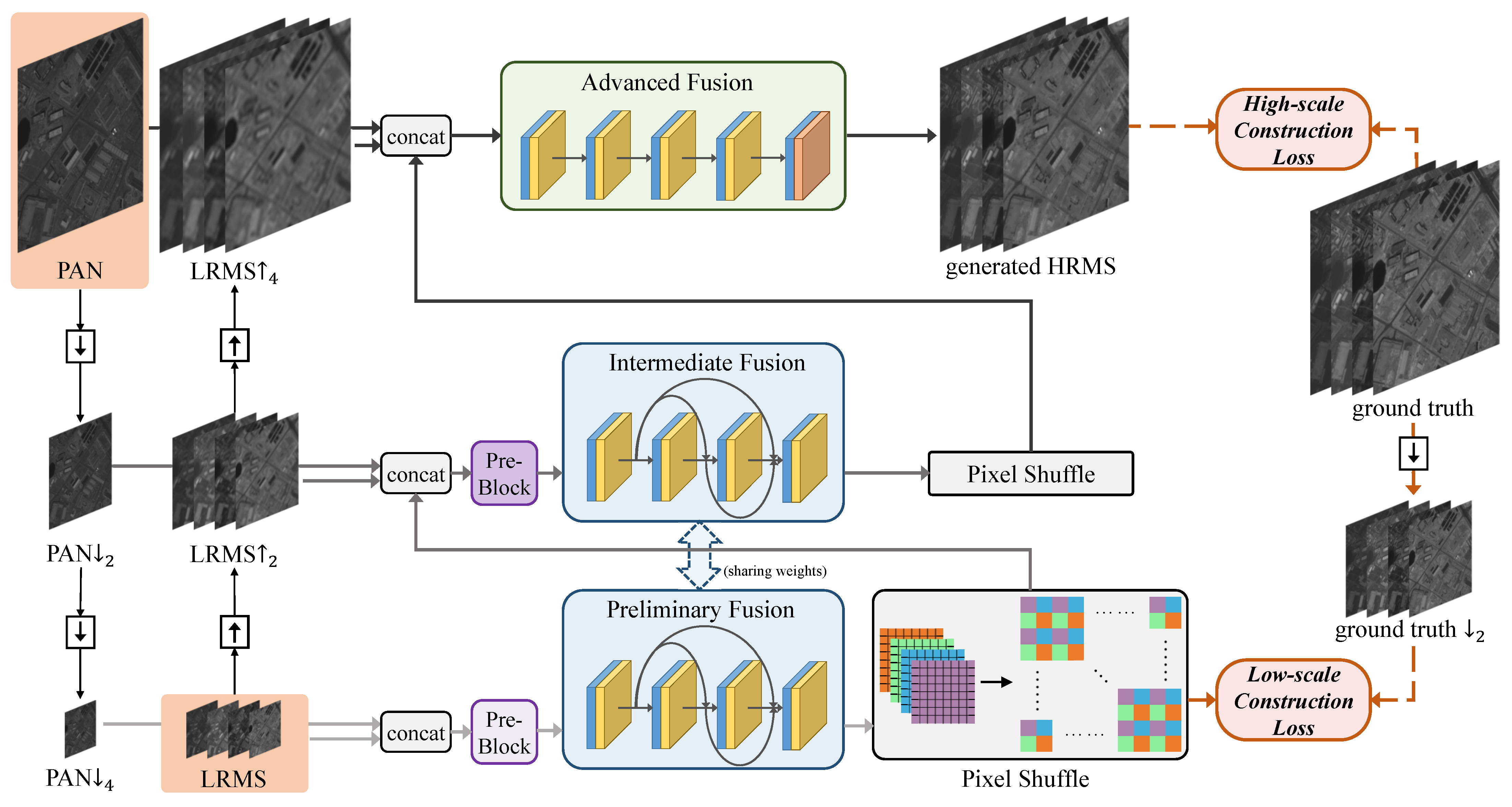
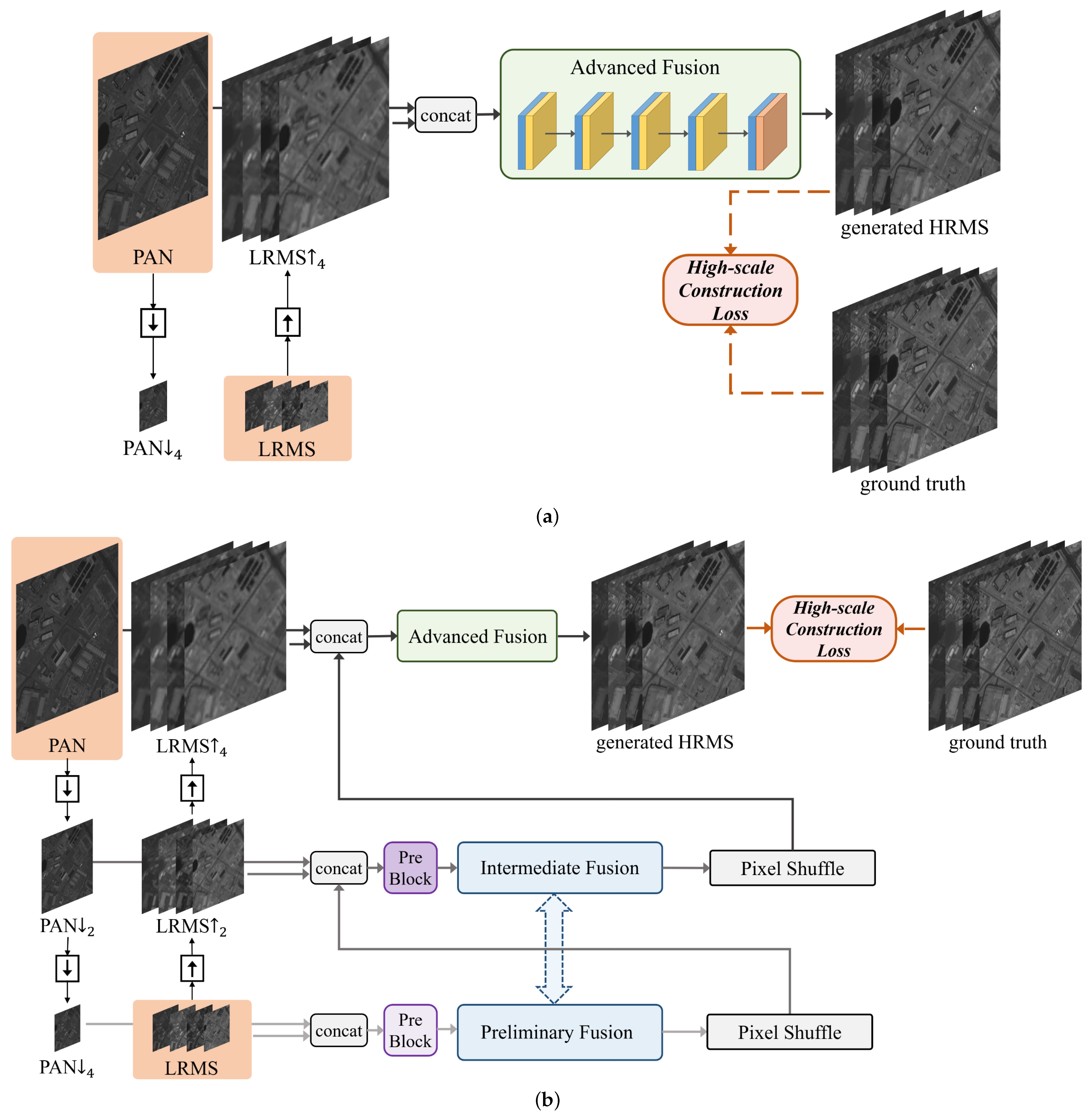
A cross-direction and progressive network, termed CPNet, is proposed for pan-sharpening to settle the issues in the prior works as mentioned above. Specifically, the “cross-direction” refers to the cross-direction processing of source images (down-sampling for PAN image and up-sampling for LRMS images) to construct three multi-scale inputs. At the same time, “progressive” means that the final fused image, i.e., the HRMS image, is generated progressively. The whole framework of the proposed CPNet is illustrated in Figure 1. In our model, we construct three multi-scale inputs with cross-direction processing of the source images.
The three-scale inputs are input into different networks (preliminary, intermediate, and advanced fusion modules) for processing, thus, making the best of the multi-scale information contained in the source images. Beyond that, the progressive reconstruction loss (including low-scale and high-scale reconstruction loss) boosts the training in all aspects of the network and promotes the fused HRMS image to approach the ground truth. In addition, since our model extracts and reconstructs both the spatial and spectral information at different scales in each image, it avoids the loss of spatial and spectral information due to insufficient information processing to the greatest extent.
The main contributions of this work are summarized as follows:
- Through the cross-direction processing of source images and the progressive reconstruction of the HRMS image, we propose a cross-direction and progressive network (CPNet) for pan-sharpening, which can fully process the source images’ information at different scales.
- The progressive reconstruction loss is designed in our model. It can boost the training in all aspects of the network to avoid the inactivation of partial networks. For another thing, it ensures a high degree of consistency between the fused image, i.e., the HRMS image, and the ground truth.
- Compared to the prior state-of-the-art works in great experiments, the proposed CPNet shows great superiority in both intuitive qualitative results and conventional quantitative metrics.
The rest of this paper is organized as follows. In Section 2, we introduce the background material and some related works of traditional and deep-learning-based pan-sharpening methods. In Section 3, the proposed CPNet is described in detail, including the problem formulation, the designs of network architecture, and the definition of loss functions. In Section 4, we present the details of the data set and training phase. The results of the qualitative and quantitative comparisons are shown subsequently. Furthermore, the ablation experiments are performed to further highlight the contributions of certain components, including the multi-scale network and progressive construction loss in our model. Our conclusions are provided in Section 5.
2. Related Work
This section introduces background material and related works, including traditional and deep-learning-based pan-sharpening methods.
2.1. Traditional Pan-Sharpening Methods
With the fast-growing demand for pan-sharpening techniques, traditional methods have been developed to achieve it in recent decades. They can be divided into four categories according to the corresponding principles, including methods based on component substitution, methods based on multi-scale decomposition, methods based on models, and hybrid methods. Next, we will introduce their main ideas.
(1) Methods based on component substitution: These methods are the most classical pan-sharpening techniques, including intensity-hue-saturation (IHS) [20], principal component analysis (PCA) [21,22], etc. They are usually achieved by flexibly transforming and replacing certain components in the transform domain, and the fused image is finally obtained by inverse transformation. High efficiency, easy implementation, and high fidelity of spatial information are the three most prominent advantages; however, they will suffer from serious spectral distortions.
(2) Methods based on multi-scale decomposition: Similar to other image fusion methods, decomposition, fusion, and transform are the main three steps in this category of pan-sharpening methods. The typical multi-scale decomposition-based methods include principle component analysis [23], contourlet [24], nonnegative matrix factorization [25], and pyramid [26,27].
(3) Methods based on models [28]: Most of the model-based methods suppose that the PAN image could be modeled as the linear association between all bands of the HRMS image, as well as the gradient maps, and the preservation of spatial and spectral information is commonly optimized by modeling. The classic model-based methods include the minimum mean-square-error sense optimum methods and the sparsity regularization-based methods.
(4) Hybrid methods [29]: This category of methods mainly combines the advantages of the existing pan-sharpening method to achieve a better fusion performance. For example, the fusion based on curvelet and ICA is one representative that combines the advantages of both component substitution and multi-scale decomposition-based methods.
The main difficulty of the existing traditional pan-sharpening methods lies in constructing between the source images and the fused image. In our work, highly non-linear mapping of the convolutional neural network is used to establish the connection between them. Through the supervised manner, the generated HRMS image is forced to maintain a high degree of consistency with the ground truth.
2.2. Deep Learning-Based Pan-Sharpening Methods
In recent years, due to the continuous advancement of deep learning technology and its continuous improvement of data processing [15,30], automatic feature extraction, and characterization capabilities, pan-sharpening methods based on deep learning have been continuously proposed, which have shown better fusion performance than the traditional methods [31]. The current deep learning methods used for pan-sharpening are mainly based on convolutional neural networks (CNN) [32] and generative adversarial networks (GAN) [33].
In CNN-based methods, Masi et al. [34] solved the pan-sharpening problem with CNN in a supervised manner. Based on this, accompanied by domain-specific knowledge, the PanNet [35] was proposed to focus on the preservation of spectral and spatial information, which improved the fused results. In addition, Zhong et al. [36] provided a hybrid pan-sharpening method, which combined the advantages of CNN and Gram–Schmidt transformation.
In addition, aiming at taking full advantage of the high nonlinearity of deep learning, residual learning between the LRMS and ground truth was adopted to establish a deep convolutional neural network in DRPNN [37]. Similarly, the CMC proposed by Wei et al. [38] solved the pan-sharpening problem from the perspective of improving the network structure with a two-stream deep learning architecture. Fu et al. [39] proposed a two-path network with feedback connections to make full use of the powerful deep features, while Zhou et al. [40] designed an unsupervised perceptual pan-sharpening framework based on auto-encoder and perceptual loss.
As for the GAN-based methods, Liu et al. [41] presented PSGAN to generate high-quality pan-sharpened images through adversarial learning between the generator and discriminator, which was also the first GAN-based pan-sharpening method. Furthermore, the RED-cGAN [42] was proposed with the residual encoder–decoder module extracting multi-scale features, and the discriminator was utilized to enhance the spatial information further. Innovatively, a GAN was employed without supervision in Pan-GAN proposed by Ma et al. [43]. In this model, the adversarial relationship is established between a generator and two discriminators, where the two discriminators are used to preserve the spectral and spatial information.
In our work, the proposed CPNet is the pan-sharpening method based on CNN. Additionally, compared with the existing deep-learning-based pan-sharpening methods, the information in the source images can be fully extracted and reconstructed at different scales in our model.
3. Proposed Method
In this section, we describe the proposed CPNet in detail. We first present the problem formulation and then introduce the design of network architectures. Finally, the definition of loss functions is given.
3.1. Problem Formulation
Pan-sharpening aims to preserve as much spatial and spectral information as possible from the source images by fusing the PAN and the LRMS image. For this purpose, the processing, including the extraction and reconstruction of the information in the source images, is crucial. The main idea of our CPNet is to fully process the information through the cross-direction processing of source images and the progressive reconstruction of the HRMS image.
As shown in the brown background images in Figure 1, the LRMS image and the high-resolution PAN image were the source images with the size of and , respectively. W and H were the width and the height of the LRMS image. N was set as 4, meaning the number of bands, and r was set as 4, expressing the spatial resolution ratio between the PAN image and the LRMS image.
To take full advantage of the related information of the PAN and LRMS images across different scales, three multi-scale inputs are constructed with the cross-direction processing of them (down-sampling for PAN image and up-sampling for the LRMS image): PAN and LRMS; PAN and LRMS; and PAN and LRMS. Our model has three fusion stages, which, respectively, correspond to the modules of preliminary fusion, intermediate fusion, and advanced fusion.
The fusion idea of CFNet is as follows: after being upsampled by pixel shuffling, the output of the current fusion stage is used as the input of the next fusion stage together with the source images of larger scale. The final fused image, i.e., the HRMS image, is generated progressively, that is, a low-scale fused image, i.e., the HRMS image, is generated in advance before the final output.
The generated HRMS and HRMS images are constrained by ground truth and ground truth with the high-scale construction loss and the low-scale construction loss. Both of them constitute the progressive reconstruction loss. The progressive reconstruction loss not only boosts the training in all aspects of the network, especially in the preliminary fusion stage, but also ensures a high degree of consistency between the fused image, i.e., the HRMS image, and the ground truth.
3.2. Network Architectures
The modules of preliminary fusion, intermediate fusion, and advanced fusion represent the three stages of the fusion process. The preliminary fusion and intermediate fusion modules have the most similar functions. To improve the utilization of the fusion module and reduce the network parameters, the network architectures of the preliminary fusion and intermediate fusion modules are consistent and share the same weights. Next, we will introduce the network architectures of the pre-block, the Preliminary/Intermediate, and advanced fusion modules in detail.
3.2.1. Network Architecture of the Pre-Block
The two pre-blocks were used to preprocess the concatenated data, and then the output of the Pre-block was used as the input of initial training/intermediate training. Each pre-block contained two convolutional layers with the kernel size and stride set as and 1. The numbers of output channels of the two convolutional layers were 16 and 32, respectively.
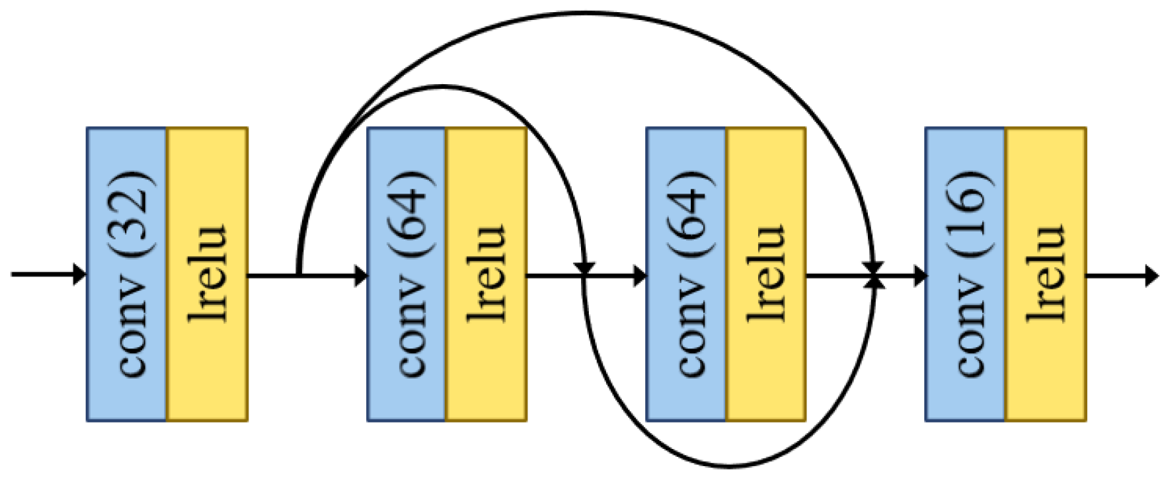
3.2.2. Network Architecture of the Preliminary/Intermediate Fusion Module
The network architecture of the preliminary/intermediate fusion module is shown in Figure 2. The fusion module was mainly used for the progressive reconstruction of the output images. There are four convolution layers, and the design of the network architecture draws from the concept of DenseNet [44].
Specifically, as a feed-forward style, each layer was directly connected with other layers. The reference of dense blocks further enhances the utilization of features and alleviates the problem of gradient disappearance in the training process [45]. Moreover, we set the padding mode of all convolution layers as “REFLECT”. Notably, we set all the kernel size as and the stride as 1. The Leaky ReLU was employed as the activation function in all convolutional layers.
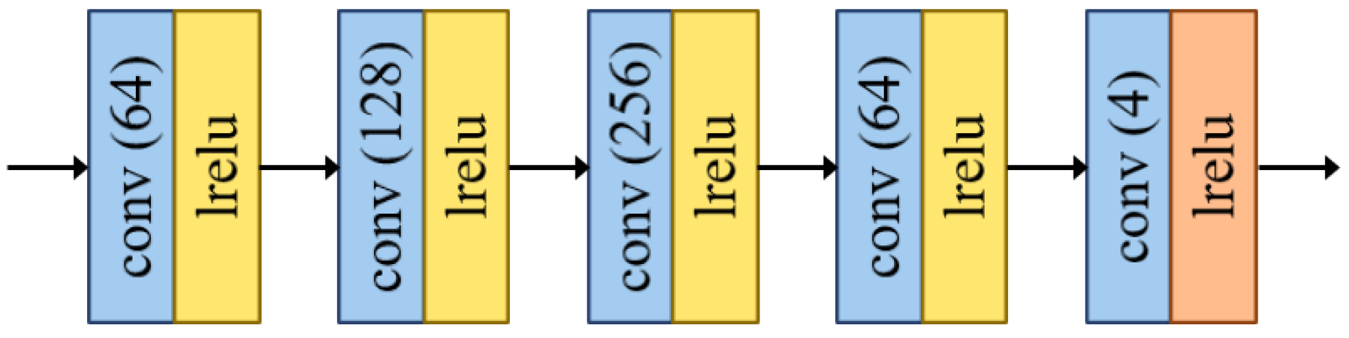
3.2.3. Network Architecture of the Advanced Fusion Module
The network architecture of the advanced fusion module is shown in Figure 3, which is composed of five convolutional layers. The advanced fusion module is responsible for integrating multi-scale information and dimensionality reduction and outputs the generated HRMS image. Consistent with the network architecture of the preliminary/intermediate fusion module, the padding mode of each convolutional layer was set as “REFLECT”, and the kernel size was set as with the stride setting as 1. The first four convolutional layers adopted Leaky ReLU as the activation function, while for the last layer, it was activated by tanh.
3.3. Loss Function
The loss function determines the direction and degree of the network optimization. In our CPNet, the direction and degree of the network optimization was determined by the progressive reconstruction loss. This can boost the training in all aspects of the network to avoid the inactivation of partial networks. This ensures a high degree of consistency between the fused image, i.e., the HRMS image, and the ground truth. The progressive reconstruction loss consisted of the high-scale reconstruction loss and the low-scale reconstruction loss , which is defined as follows:
where the is the weight controlling the trade-off between them.
Specifically, the high-scale reconstruction loss was employed to constrain the generated high-scale fused image, i.e., the HRMS image, with the high-scale ground truth. Consequently, the generated HRMS image could maintain a high degree of consistency with the ground truth. The high-scale reconstruction loss is mathematically given by:
where the is the operation taking the absolute value. denotes the generated HRMS image, and G denotes the ground truth.
The low-scale reconstruction loss was employed to constrain the generated low-scale fused image, i.e., the HRMS image with the low-scale ground truth, i.e., ground truth. In other words, it can boost the training in all aspects of the network to avoid the inactivation of partial networks. The low-scale reconstruction loss is mathematically formulated as follows:
4. Experiments and Analysis
In this section, abundant experiments were conducted to verify the performance of the proposed CPNet. First, we introduce the experimental settings, including the data set, training details, comparison methods, and evaluation metrics. Second, not only the visual inspection comparison but also the quantitative comparison were performed to validate the superiority of our CPNet. We also performed ablation experiments to illustrate the specific effects of including the multi-scale network and progressive construction loss in our method.
4.1. Experimental Design
4.1.1. Data Set and Training Details
The satellite images used for training and testing our CPNet were from the data set. The characteristics of sensors, including spatial resolutions and spectral bands, are reported in Table 1. Due to the lack of HRMS images in practice, we obtained the HRMS image following Wald’s protocol [46]. Specifically, the original PAN and MS images were down-sampled into the lower resolutions, and the original MS image was used as the ground truth. In our work, the spatial resolution ratio r of the PAN image and the LRMS image was 4.
First, the down-sampled PAN and LRMS images were cropped into patches of and , respectively. Secondly, we obtained the ground truth by cropping the original LRMS into patches of size . Finally, the training data containing 2052 patch pairs was established. Furthermore, in Equation (1), the hyper-parameter was set as 0.5.
The number of training epochs was 10, and the batch size was set as 8. The parameters in our model were updated by the AdamOptimizer. The experiments were performed on a 3.4 GHz Intel Core i5-7500 CPU and NVIDIA GeForce GTX Titan X GPU. This algorithm was realized using the TensorFlow platform. The overall description of the proposed method is summarized as Algorthm 1.
4.1.2. Comparison Methods
To verify the effectiveness of the proposed CPNet, we chose eight state-of-the-art pan-sharpening methods to compare with it. The comparison methods comprise PRACS [47], PNN [34], PanNet [35], PSGAN [41], TACNN [48], LGC [49], Pan-GAN [43], and SDPNet [13]. More concretely, PRACS and LGC are two typical traditional methods, while the others are six typical methods based on deep learning.
As for the traditional methods, PRACS is a relatively recent method among the most commonly used competitive methods. LGC is the first method that considers the gradient difference of PAN and HRMS images in different local patches and bands rather than only uses global constraints. Thus, it can achieve accurate spatial preservation.
The comparative deep-learning-based methods can be divided into two categories. For one thing, according to whether there exist ground-truth HRMS images for supervised learning, the deep-learning-based methods can be divided into supervised methods and unsupervised methods. For supervised methods, we selected PNN, PanNet, PSGAN, TACNN, and SDPNet as representative methods. Among them, PNN is the first deep-learning-based method for pan-sharpening, which is a foundation and landmark method.
Considering that PNN directly inputs source images, which fails to exploit known image characteristics to define the network structure, PanNet trains the network in the high-pass filtering domain to preserve the spatial details. In addition, some methods use different architectures, loss functions, or training mechanisms to protect the information in source images. For instance, TACNN modifies the loss function using loss and modifies the architecture by working on image residuals and deeper architectures. PSGAN is based on generative adversarial networks (GANs).
It uses the discriminator to distinguish the differences between fused images and the ground truth to minimize their differences further. SDPNet applies both the surface-level constraint and deep-level constraint. By objectively defining the spatial and spectral information through deep networks, it can further preserve both types of information. Pan-GAN is the representative of unsupervised methods. It generates the HRMS image by constraining it to maintain the pixel intensity of the LRMS image and the gradients of the PAN image.
The generative adversarial mechanism is used to enhance information preservation. For another thing, PNN, PanNet, TACNN, and SDPNet are CNN-based methods, while PSGAN and Pan-GAN are GAN-based methods. Considering several classification ways, we select the above eight comparison methods to include methods based on various theories as far as possible.
| Algorithm 1: Overall description of CPNet. |
|
4.1.3. Evaluation Metrics
In quantitative comparisons, we also used five commonly used metrics to evaluate the quality of the fused image, including the relative dimensionless global error in synthesis (ERGAS) [50], the root-mean-squared error (RMSE), the structural similarity (SSIM) [51], the spectral angle mapper (SAM) [52], and the spatial correlation coefficient (SCC) [53]. Except for SCC, which is a non-reference metric, the rest are full-reference metrics. The specific introductions of these metrics are as follows:
- The ERGAS is used as a global metric, measuring the mean deviation and dynamic range change between the fused result and ground truth. Therefore, the smaller value of the ERGAS means that the fused image is closer to the ground truth. The ERGAS is mathematically defined as follows:where r is set as 4 in our work, expressing the spatial resolution ratio between the PAN image and LRMS image, and N is 4, denoting the number of the band of LRMS. We use the to compute the root mean square error between the fused result and ground truth, and the expresses the average of the ith band in the source LRMS image.
- The RMSE shows the difference between the fused result and ground truth through the change of pixel value. The smaller RMSE denotes that the pixel between the fusion image and the ground truth is closer. The RMSE is mathematically formulated as follows:where h and w indicate the height and weight of the LRMS image, respectively. The G and F are the ground truth and fused image.
- The SSIM is the metric measuring the structural similarity between the fused result and the ground truth. It evaluates the structural similarity in three different factors containing brightness, contrast, and structure. The higher the SSIM is, the more the fused image has higher structural similarity with the ground truth. The SSIM between the fused result F and the ground truth G is mathematically formalized as follows:where the g and f are, respectively, the image patches of the ground truth G and fused image F. The and are the mean value and standard deviation, respectively. The , and are the parameters stabilizing the metric.
- The SAM reflects the spectral quality of the fused result by calculating the angle between the fused result and ground truth, and the calculation is performed between each pixel vector in n-dimensional space and the endmember spectrum vector. The smaller SAM expresses that the fused image possesses a higher consistency with the ground truth in spectral information. The SAM is mathematically given by:
- The SCC embodies the correlation in spatial information between the fused result and the PAN image, and thus the ground truth is not needed as a reference. The larger value of SCC means that the fused image shows better performance in preserving spatial information.
4.2. Results of Reduced-Resolution Validation and Analysis
4.2.1. Qualitative Comparison
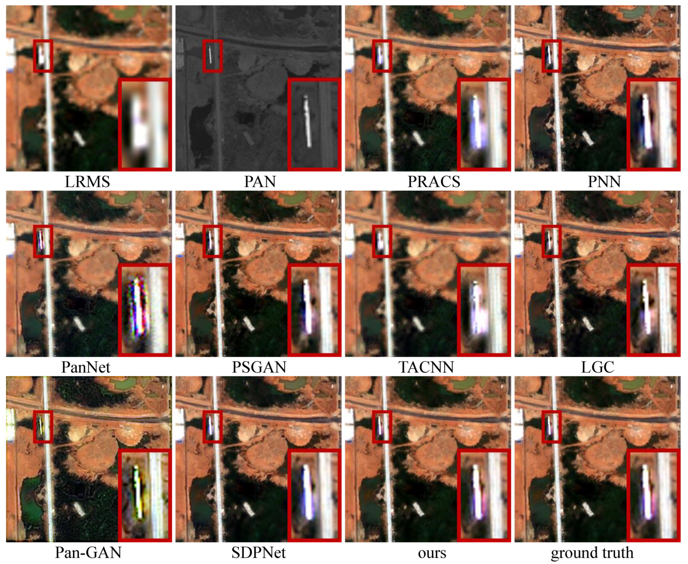
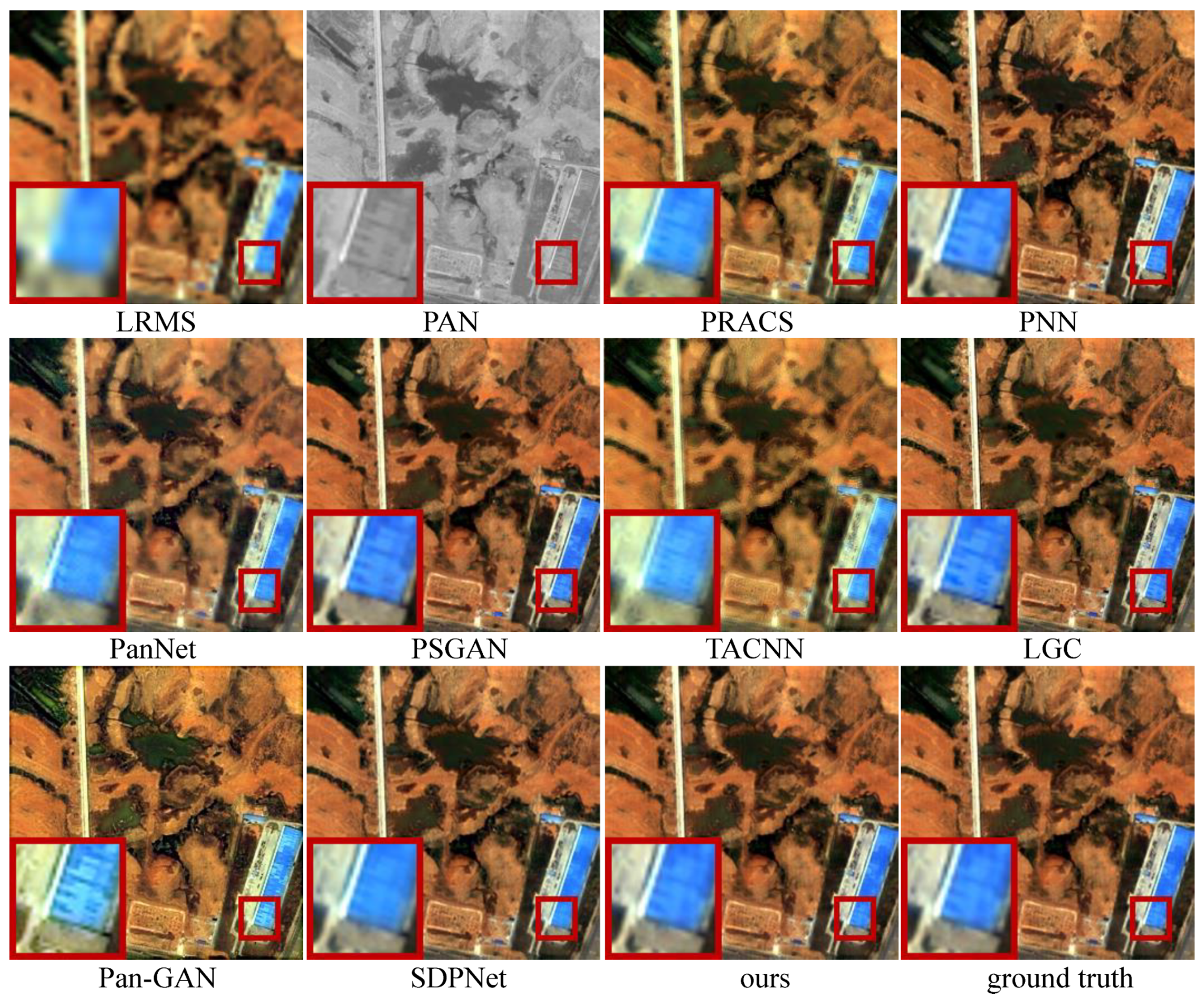
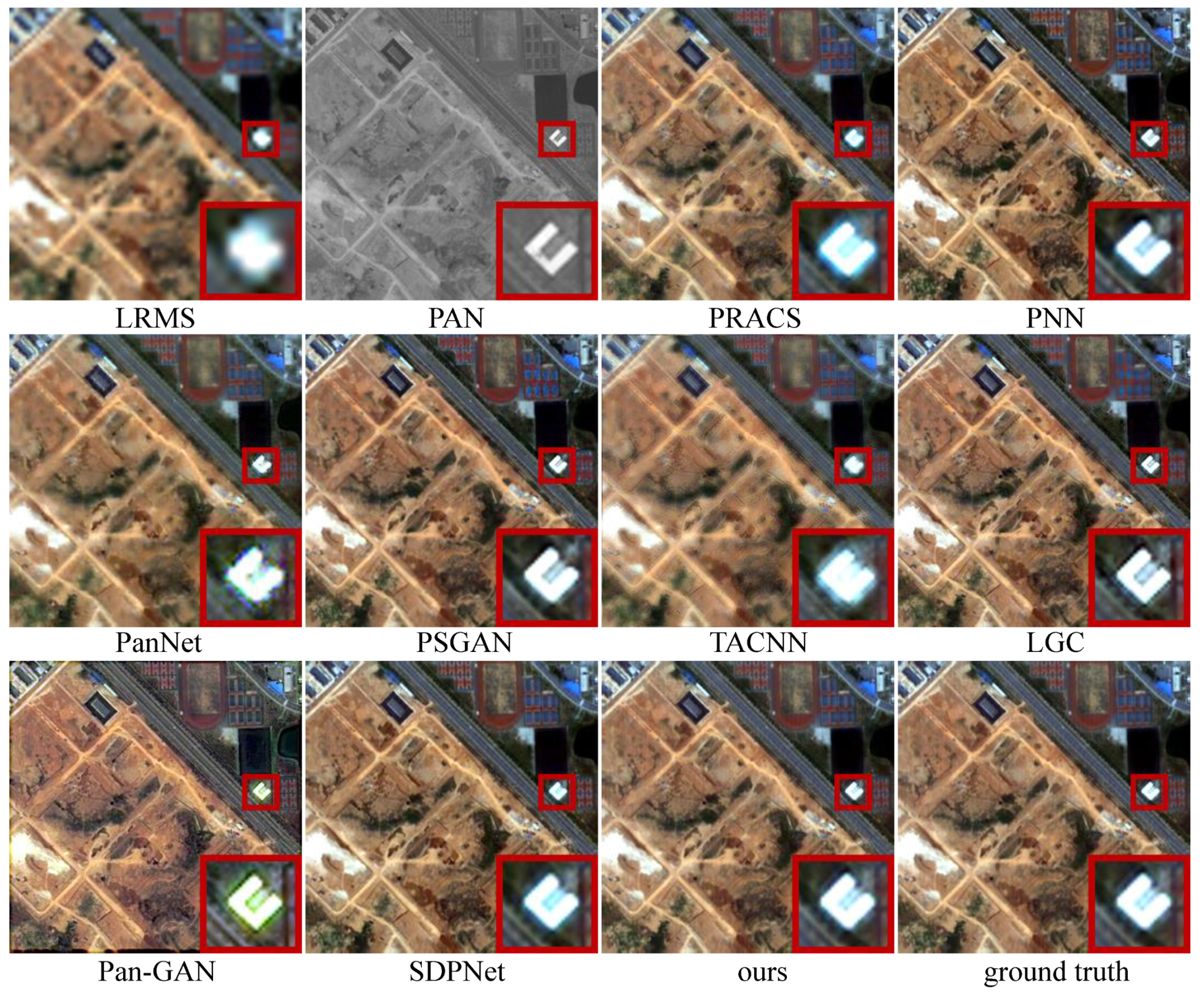
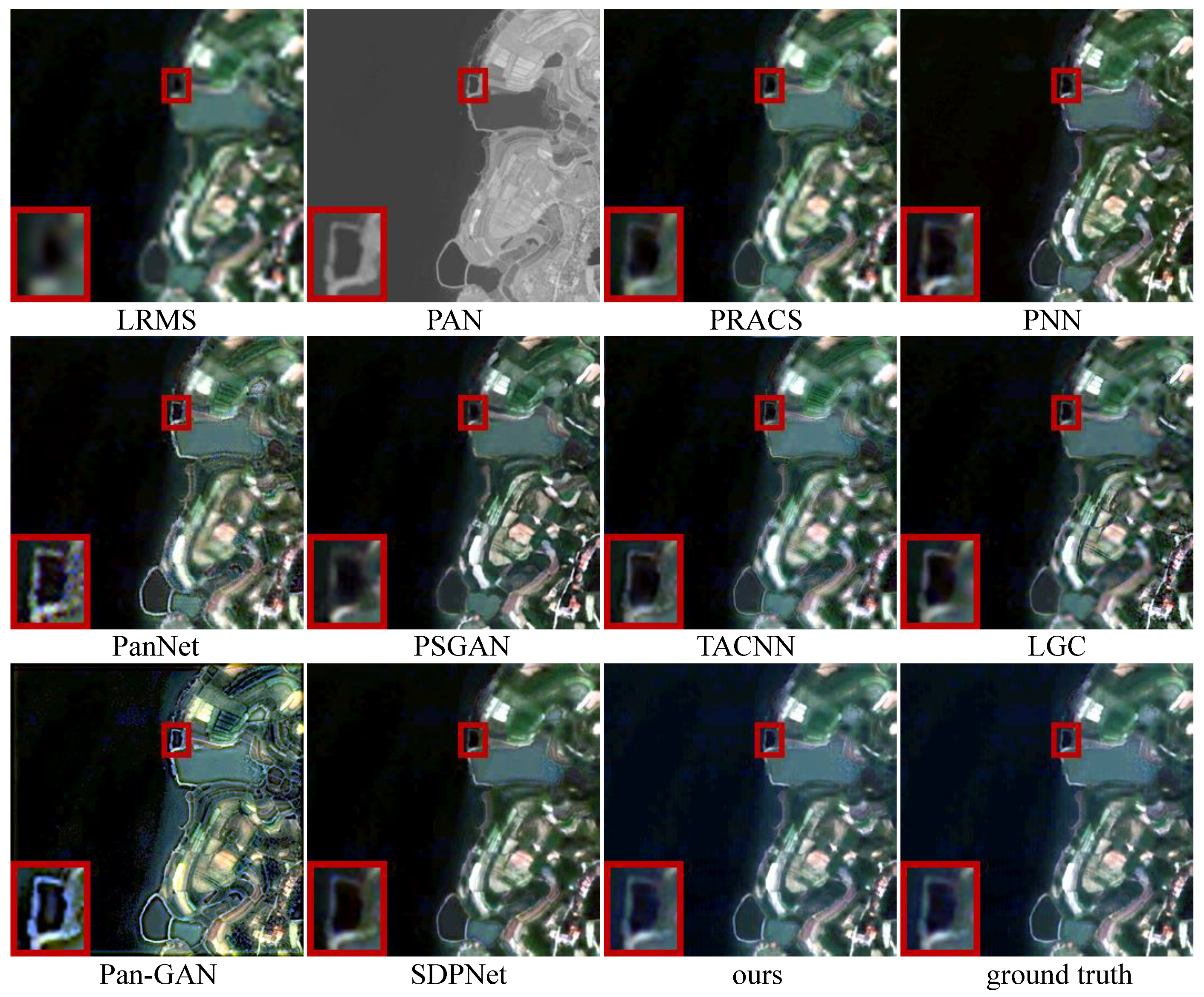
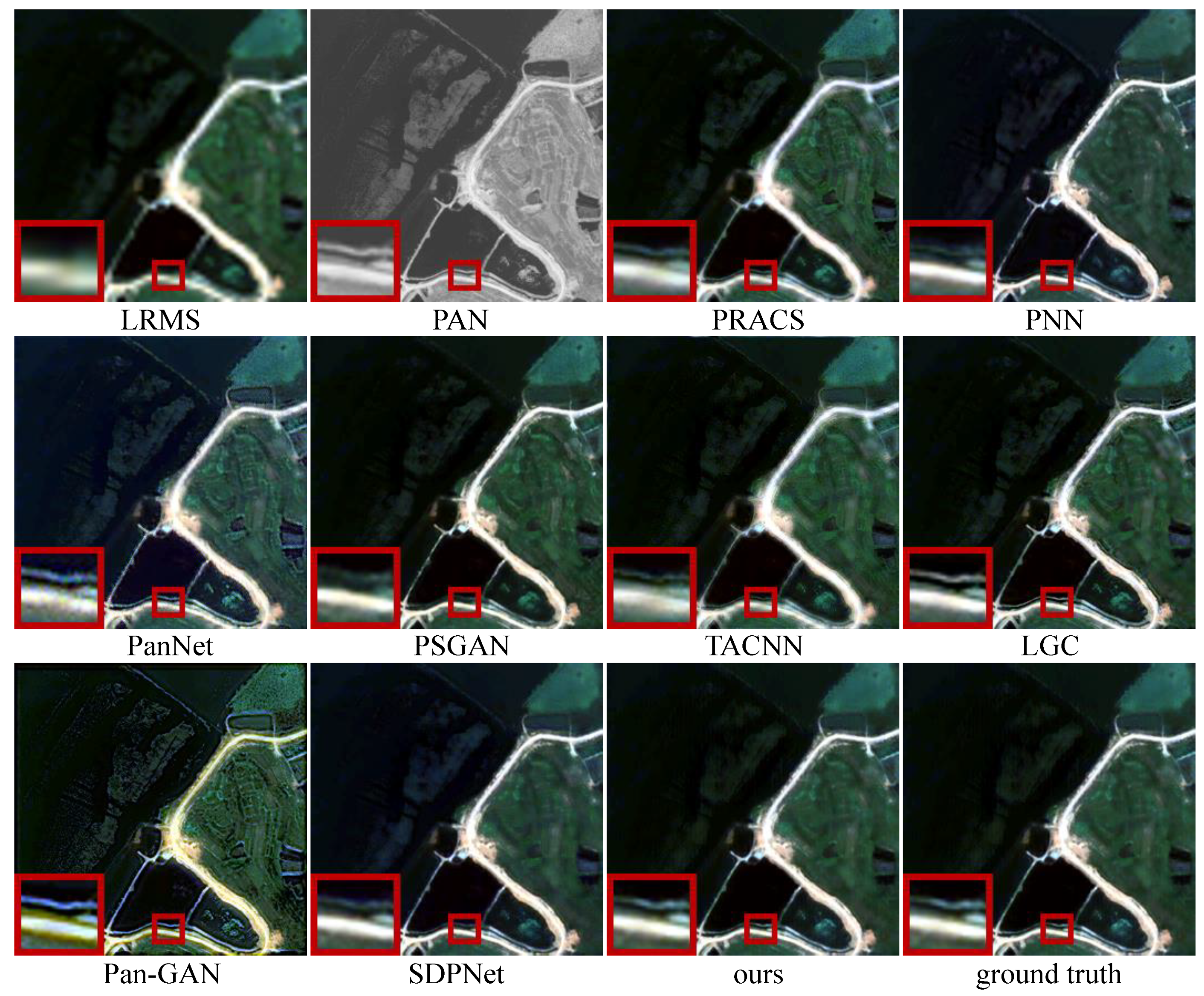
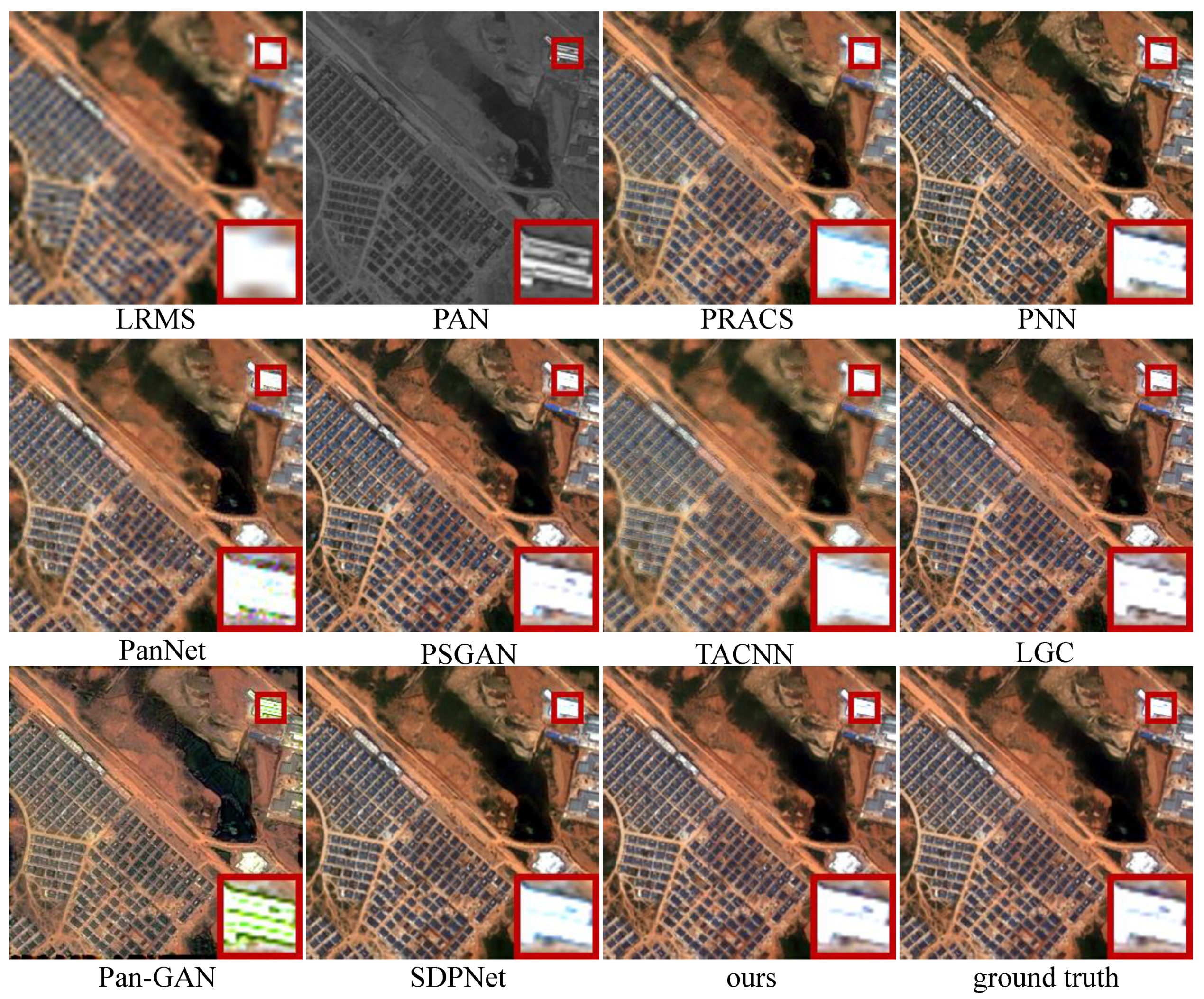
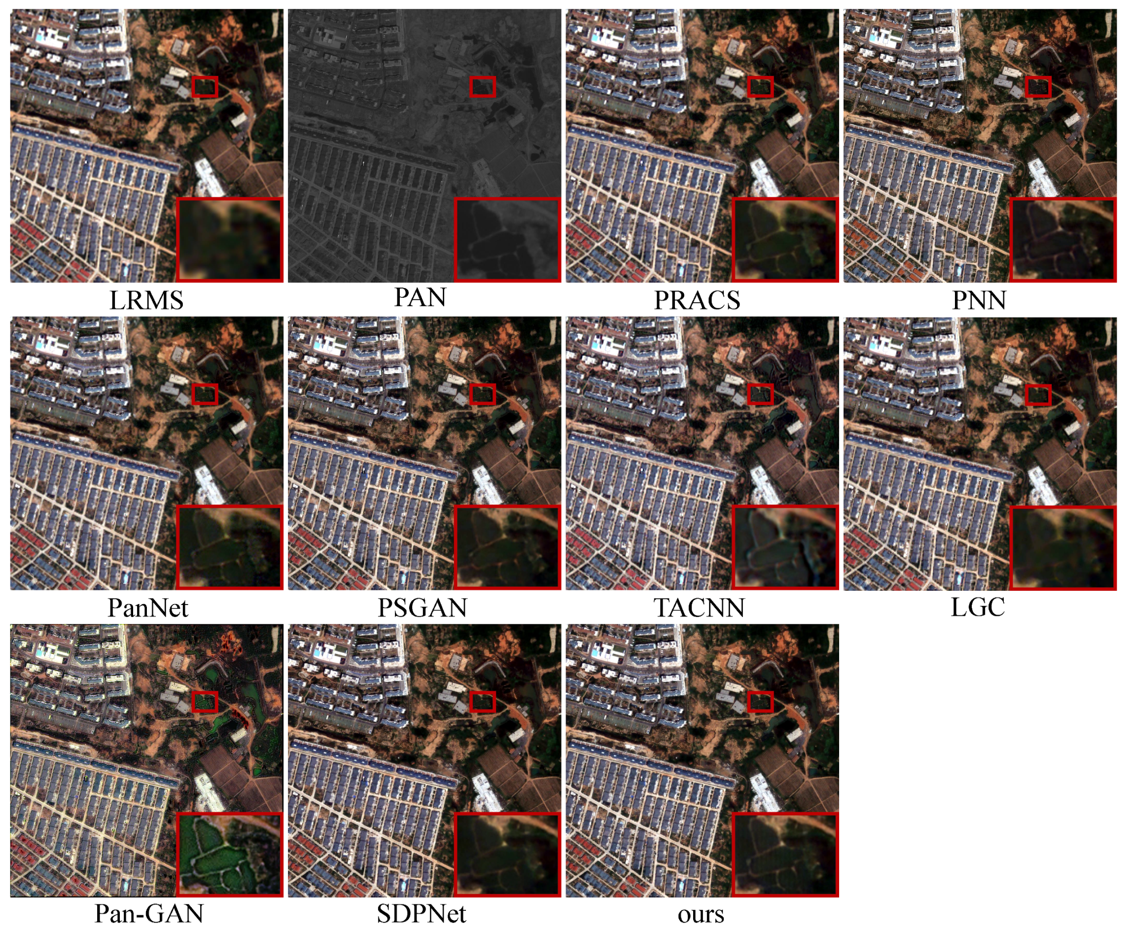
- Results. In qualitative comparison, to have better visualization and perception, we choose the first three bands (including the blue, green, and red bands) of the LRMS, generated HRMS images, and ground truth for presentation. The intuitive results on six typical satellite image pairs are illustrated in Figure 4, Figure 5, Figure 6, Figure 7, Figure 8 and Figure 9.
- Analysis. The fused results of each pan-sharpening method have approximately the same style in these six typical satellite image pairs. For PRACS, PNN, PanNet, and TACNN, on the one hand, the severe spatial distortion appears in all the six examples, shown as edge distortion or blurred texture details. On the other hand, they suffer from varying degrees of spectral distortion and show distinct differences in spectral information from the ground truth. In addition, the results of PanNet introduce significant noise.The Pan-GAN preserves the spatial and spectral information based on the constraints of the gradient and pixel intensity between the fused result and source images. Nevertheless, the excessive gradient constraint and the distinguishing between the fused result and the ground truth led to the most serious spectral distortion in these pan-sharpening methods in Figure 4, Figure 5, Figure 6, Figure 7, Figure 8 and Figure 9, as well as edge distortion, as shown in Figure 4.In PSGAN, LGC, and SDPNet, Although their fused results show approximately the same spectral information as the ground truth, their spatial information is still lacking compared to the ground truth, showing varying degrees of blurry texture details or edge distortion. The result of SDPNet in Figure 9 does not preserve the spectral information well. By comparison, the results of our CPNet do not undergo the questions as mentioned above and can better maintain the spatial and information simultaneously, showing the best qualitative results.
4.2.2. Quantitative Comparison
- Results. In order to have a more objective evaluation of the performances of these pan-sharpening methods, we further performed the quantitative comparison of our CPNet and the eight competitors on eighty satellite image pairs in the testing data. The statistical results are provided in Table 2.
- Analysis. As provided in the table, our CPNet achieved the best values in three out of five metrics, including the ERGAS, RMSE, and SSIM. In terms of the remaining two metrics, our CPNet can still reach the second-best value in SAM and the third value in SCC, respectively. To be more specific, the best value in ERGAS revealed that the mean deviation and dynamic range changes between the fused result and ground truth were the least, and the best value in RMSE indicates that the pixel change of our fused results was the smallest.The best value in SSIM demonstrates that the results of our CPNet showed the highest structural similarity with the ground truth. The second-best value in SAM also showed that our CPNet generated comparable results in preserving spectral information. Last, since the methods Pan-GAN and LGC both focus on imposing gradient constraints between the PAN image and the fused results, they preserved the spatial information well, which led to better results in SCC for PAN-GAN and LGC.However, they do not consider the preservation of the spectral information, and the transitional constraint on the gradient even caused edge distortion in some results. Therefore, with the comprehensive evaluation on all the five metrics, we concluded that our CPNet performed the best in preserving both spatial and spectral information in general.
4.2.3. Reliability and Stability Validation
To analyze and validate the reliability and stability of the proposed method, we used the independent samples t-test to validate whether there were performance differences between the training data and test data. For this purpose, we measured the performance of the proposed method on 222 training patch pairs. For higher accuracy, the results on four reference metrics were used for validation. The results are shown in Table 3.
For the results of each metric, we set the null hypothesis as that no statistically significant difference between the performance on the training data and that on the test data. In our experiment, the degree of freedom (df) was 150, and this is a two-tailed test. When we set the probability level as and performed the two-tailed test, the corresponding critical t-value was 1.9679. As shown in Table 3, the calculated t-values of the four metrics were all smaller than the critical value. Thus, we do not reject the null hypothesis. In other words, there was no statistically significant difference between the performance on the training data and that on the test data.
4.3. Results of Full-Resolution Validation and Analysis
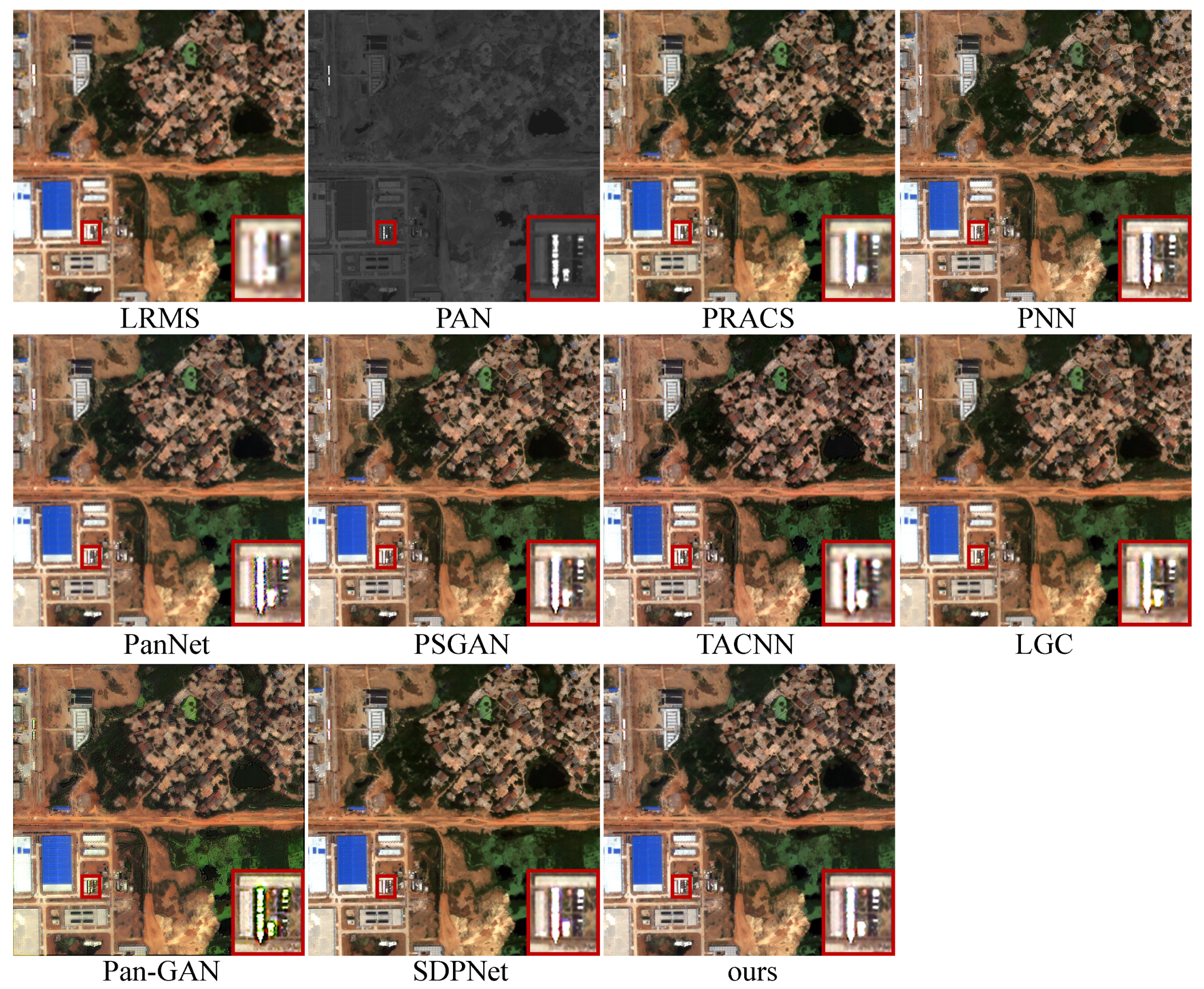
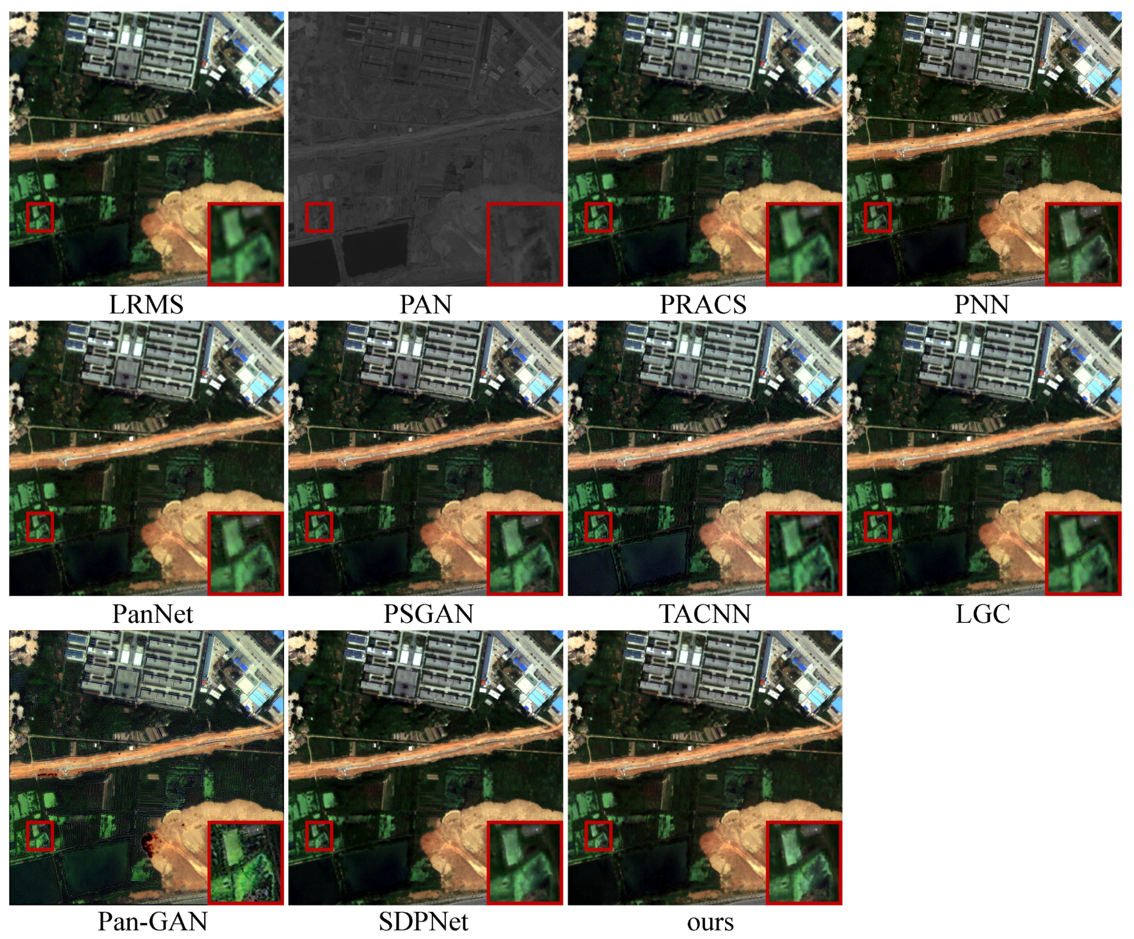
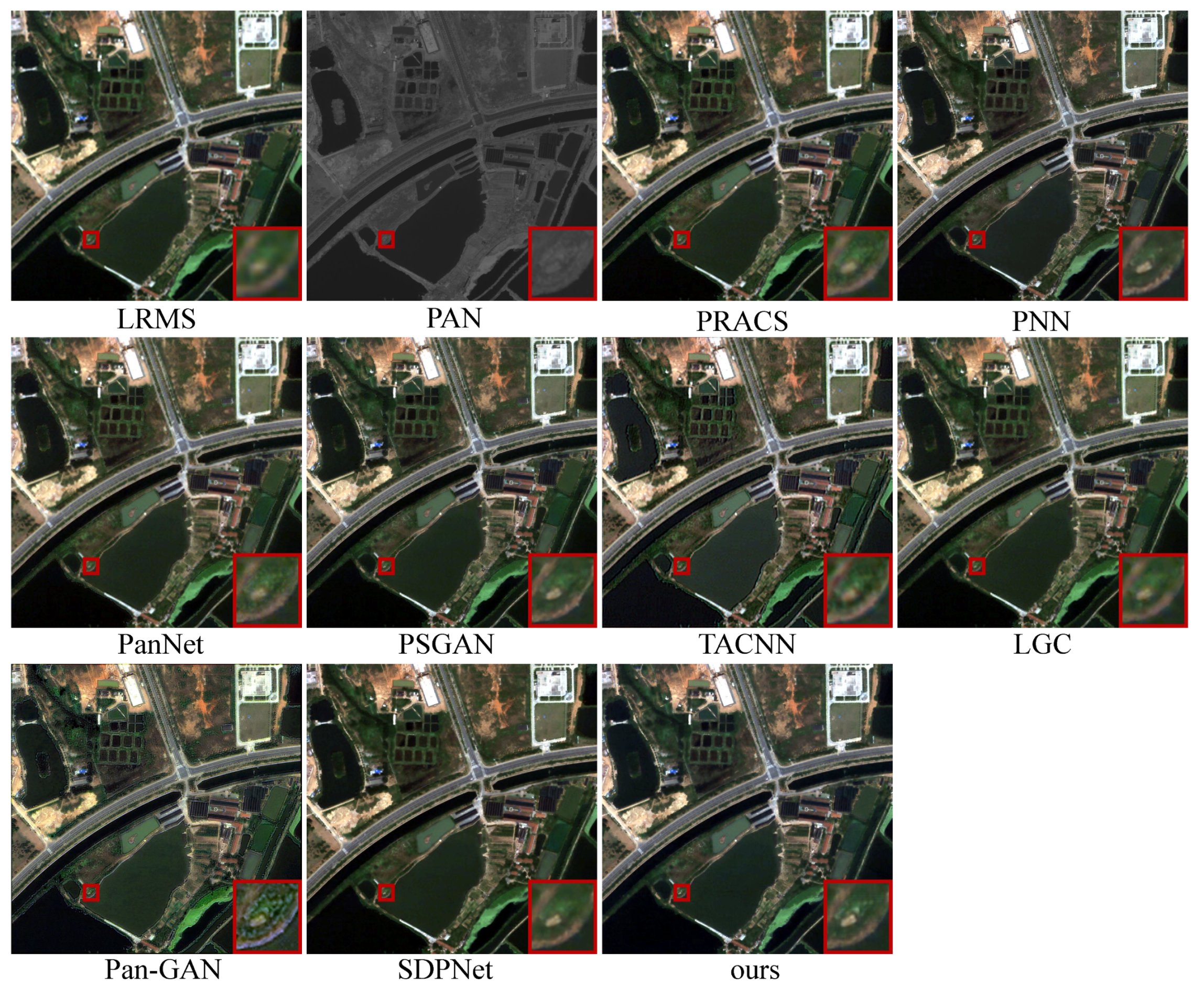
- Results. To verify the application of our CPNet on full-resolution data, we further performed qualitative experiments, whose source PAN and LRMS images were at the original scale, and hence there was no ground truth. The comparison results are presented in Figure 10, Figure 11, Figure 12 and Figure 13.
- Analysis. Equally, the results of our CPNet achieved outstanding performance. As shown in Figure 10, our fused result can describe the edge of the buildings most clearly, while the results of other methods have varying degrees of edge blur. The problem of spectral distortion still exists in the results of other methods. The result of PanNet also exposes the problem of noise introduction and the severest spectral distortion in the result of Pan-GAN.A similar situation also appears in other full-resolution satellite image pairs as displayed in Figure 11, Figure 12 and Figure 13. In conclusion, our CPNet also showed the best fusion performance in the full-resolution results, which is reflected in the spatial and spectral information preservation.
4.4. Ablation Study
We performed the multi-scale network and progressive construction loss in the proposed method to ensure high consistency between the generated HRMS image and ground truth. To validate the effectiveness of these two items separately, we performed two ablation studies in this section. First, to validate the efficacy of the multi-scale fusion network, we removed the preliminary and intermediate fusion networks as shown in Figure 1. The overall framework is shown as Figure 14a.
In this case, only the advanced fusion network was used to fuse the PAN and up-sampled LRMS images. Second, in CPNet, the progressive reconstruction loss function of the overall network consisted of two items. As shown in Equation (1), it consists of the low-scale and high-scale loss. The low-scale loss is used to boost the training in all aspects of the network to avoid the inactivation of the preliminary and intermediate fusion networks.
To validate the effectiveness of the low-scale loss, we employed the same network components and architectures with the proposed CPNet. In contrast, the total loss function only consisted of the high-scale reconstruction loss, i.e., the hyper-parameter defined in Equation (1) was set as 0. In this condition, the framework is summarized as shown in Figure 14b.
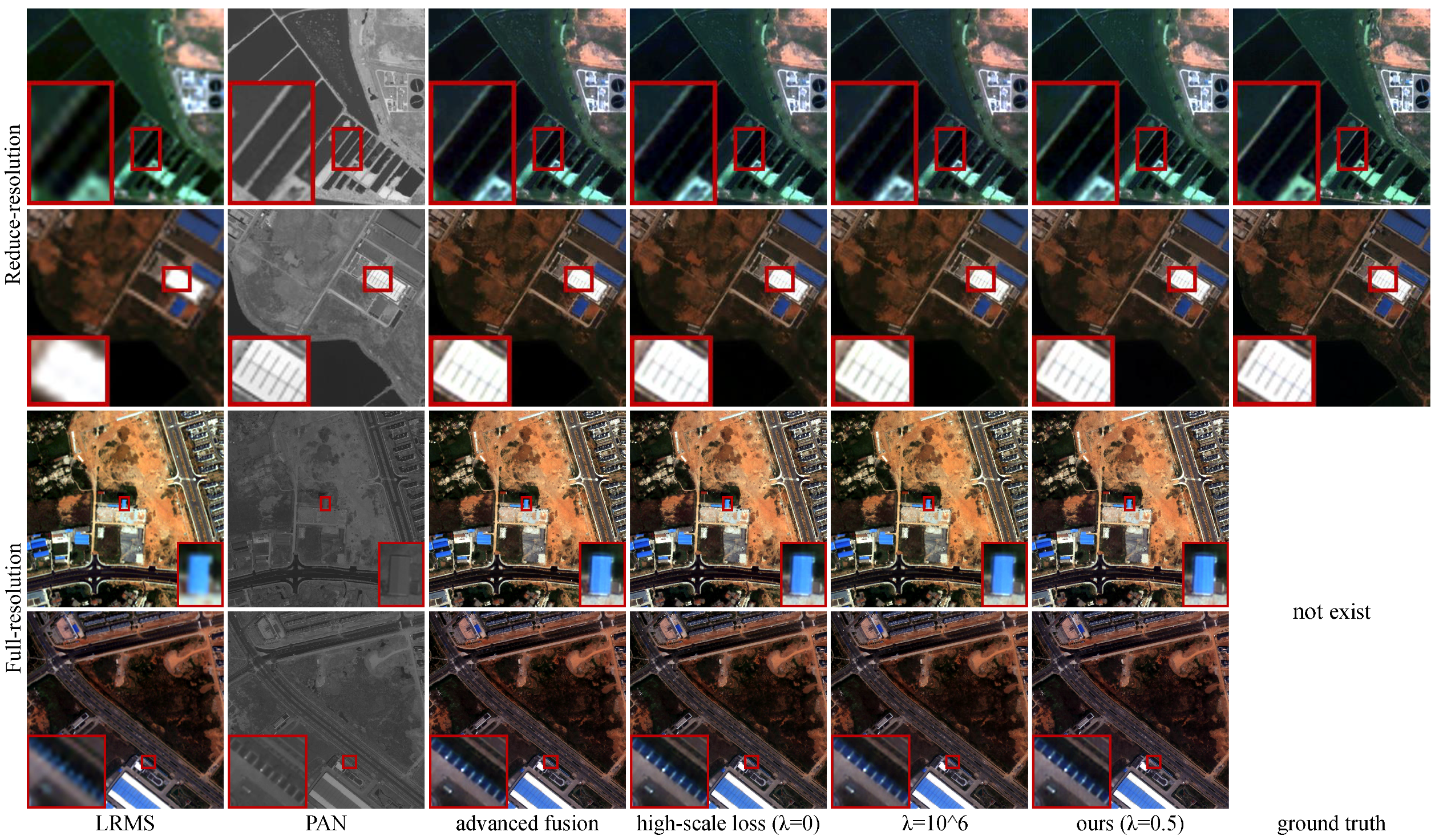
The qualitative comparison results are shown in Figure 15. The results shown in the first two rows were performed on two pairs of reduced-resolution source images, and the results in the last two rows were performed on two pairs of full-resolution source images. Thus, in the last two rows, the ground truth was not available. When only the advanced fusion network was applied, the spectral information completely came from the up-sampled multi-spectral image. As shown in the third column of Figure 1, it blurred the high-quality texture details in the PAN image. Some edges in the PAN images were weakened or even lost in the fused results.
By comparison, when the preliminary and intermediate fusion networks were applied, the multi-spectral image was sharpened from the lowest resolution, as shown in Figure 1. The progressive approach ensured that the high-quality spatial information in the PAN image was preserved to a greater extent. We concluded this from the results shown in the fourth column compared with those in the third column.
In addition, the low-scale loss function can further guarantee the function of the progressive approach. The qualitative results are shown in the fifth column in Figure 15. Compared with the results of only applying the advanced fusion network and only using the high-scale loss, the proposed CPNet exhibited the most abundant texture details, which were blurred or even not preserved in other results. The guarantee of the preliminary and intermediate network functions ensured that the output of the intermediate network retained the fundamental spatial and spectral information. Then, the advanced fusion network focused on preserving the high-quality texture details in the PAN image. Thus, the proposed method showed the most satisfactory fused results.
The quantitative results of the two ablation methods and the proposed CPNet are shown in Table 4. Considering the results of several indexes comprehensively, the method of just applying the advanced fusion network showed the worst fusion performance. The method that only applied the high-scale loss showed suboptimal performance, and our CPNet showed optimal performance. More concretely, the best results of our CPNet on ERGAS, RMSE, and SSIM showed that the similarities between the generated HRMS images and the ground truth were the highest. The best results on SAM showed that the spectral quality of our fusion results was similar to that of the ground truth. The best result of our method on SCC indicates that our results preserved the greatest extent of ground truth.
4.5. Hyper-Parameter Analysis
The hyper-parameter in the proposed method consists of defined in Equation (1), which controls the trade-off between the high-scale and low-scale constraint losses. We analyzed the effect of this hyper-parameter’s value on the pan-sharpening performance. When , it is the second ablation method shown in Figure 14b. The qualitative and quantitative results are shown in Figure 15 and Table 4. Then, we set , which corresponds to the proposed method. To further analyze the effect of , we set , and the results are shown in Figure 15 and Table 4.
When increases, the low-scale constraint gradually dominates the function of the network. The functions of pre-blocks, preliminary, and intermediate fusion blocks were consolidated. Then, the intermediate fusion results became increasingly similar to the down-sampled ground truth. However, the high-scale loss in the original resolution also increased. This led to the distortion of both high-quality spatial and spectral information, as shown in the qualitative results in Figure 15. The quantitative results are shown in Table 4 also objectively demonstrates that a larger resulted in more serve information distortion.
4.6. Efficiency Comparison
We compared the efficiency of different methods in this section. The traditional methods, including PRACS and LGC were tested on the CPU. The deep-learning-based methods, including PNN, PanNet, TACNN, Pan-GAN, SDPNet, and our methods were tested on the GPU. The specific runtimes are reported in Table 5. For the sake of comprehensiveness, both the efficiency on the reduced-resolution and full-resolution images were taken into account.
As shown in this table, for the reduced-resolution images, our method showed comparable efficiency. The runtime was on the same order of magnitude as PNN and PSGAN and ranked third among all the methods. For the full-resolution images, our CPNet ranked fourth, which also followed behind SDPNet. The reason is that, with the improvement of the spatial resolution, the preliminary fusion and intermediate fusion took more time. Despite all this, our method still took less time than PanNet, TACNN, and Pan-GAN.
4.7. Limitations and Future Works
This section discusses some limitations of this work and some future improvements. As shown in Figure 1, the progressive fusion went through two pixel shuffles. This was designed based on the assumption that the spatial resolution ratio of PAN and LRMS images was 4. When the spatial resolution ratio is larger than 4, the framework of the proposed method needs to be modified to different spatial resolution ratios.
In our future work, we will first consider the solution to the above-mentioned limitation. When the resolution ratio is larger than 4, e.g., if the ratio is 8, the intermediate fusion shown in Figure 1 would be performed twice. This handles the fusion of two intermediate-resolution images. In addition, the low-scale reconstruction loss would consist of two items, i.e., the similarity constraint between and and the similarity constraint between and .
We will apply our CPNet to more satellite imageries. On the one hand, we will apply it to satellite images containing different wavelength ranges, such as images captured by Ikonos and GeoEye-1 sensors. On the other hand, we will apply it to satellites images, including more spectral bands, such as images captured by WorldView-2 sensors, which contain eight spectral bands.
In addition to the similarity loss between the generated HRMS image and the ground truth, we also design a low-scale construction loss based on the pixel shuffle result of the preliminary fusion for an enhanced constraint. Likewise, the pixel shuffle result of the intermediate fusion can also potentially be used as an additional constraint. In our future work, we will investigate adding this additional constraint.
5. Conclusions
In this paper, we proposed a novel network called CPNet for pan-sharpening. Our model maximized the development and utilization of the information from the source image through the cross-direction processing of source images and the progressive reconstruction of the fused image. In addition, we designed the progressive reconstruction loss, including low-scale loss and high-scale reconstruction loss, to determine the direction and degree of the model optimization.
Particularly, the progressive reconstruction loss promoted the training of all fusion modules in different stages and preserved the spatial and spectral information in the generated HRMS image to the greatest extent. Rather than a single type of information, we processed the information in the image level throughout the fusion process, which avoided partial information loss. Compared with the state-of-the-art pan-sharpening methods, our CPNet showed the greatest preservation in both spatial and spectral information.
Author Contributions
All authors have made great contributions to the work. H.X. and Z.L. designed the research, performed the experiments, analyzed the results, and wrote the manuscript. J.H. and J.M. gave insightful suggestions to the work and revised the manuscript. All authors have read and agreed to the published version of the manuscript.
Funding
This research was funded by the National Natural Science Foundation of China under Grant 62075169, Grant 62003247 and Grant 62061160370, and also by the Fundamental Research Funds for the Central Universities under Grant 2042020kf0017.
Conflicts of Interest
The authors declare no conflict of interest.
References
- Palubinskas, G. Joint quality measure for evaluation of pansharpening accuracy. Remote Sens. 2015, 7, 9292–9310. [Google Scholar] [CrossRef] [Green Version]
- Blaschke, T.; Lang, S.; Lorup, E.; Strobl, J.; Zeil, P. Object-oriented image processing in an integrated GIS/remote sensing environment and perspectives for environmental applications. Environ. Inf. Plan. Politics Public 2000, 2, 555–570. [Google Scholar]
- Zhang, L.; Zhang, L.; Tao, D.; Huang, X.; Du, B. Hyperspectral remote sensing image subpixel target detection based on supervised metric learning. IEEE Trans. Geosci. Remote Sens. 2013, 52, 4955–4965. [Google Scholar] [CrossRef]
- Dian, R.; Li, S.; Kang, X. Regularizing hyperspectral and multispectral image fusion by CNN denoiser. IEEE Trans. Neural Netw. Learn. Syst. 2021, 32, 1124–1135. [Google Scholar] [CrossRef] [PubMed]
- Ghassemian, H. A review of remote sensing image fusion methods. Inf. Fusion 2016, 32, 75–89. [Google Scholar] [CrossRef]
- Thomas, C.; Ranchin, T.; Wald, L.; Chanussot, J. Synthesis of multispectral images to high spatial resolution: A critical review of fusion methods based on remote sensing physics. IEEE Trans. Geosci. Remote Sens. 2008, 46, 1301–1312. [Google Scholar] [CrossRef] [Green Version]
- Zhang, H.; Xu, H.; Tian, X.; Jiang, J.; Ma, J. Image fusion meets deep learning: A survey and perspective. Inf. Fusion 2021, 76, 323–336. [Google Scholar] [CrossRef]
- Xie, B.; Zhang, H.K.; Huang, B. Revealing implicit assumptions of the component substitution pansharpening methods. Remote Sens. 2017, 9, 443. [Google Scholar] [CrossRef] [Green Version]
- Lillo-Saavedra, M.; Gonzalo-Martín, C.; García-Pedrero, A.; Lagos, O. Scale-aware pansharpening algorithm for agricultural fragmented landscapes. Remote Sens. 2016, 8, 870. [Google Scholar] [CrossRef] [Green Version]
- Wang, P.; Zhang, G.; Hao, S.; Wang, L. Improving remote sensing image super-resolution mapping based on the spatial attraction model by utilizing the pansharpening technique. Remote Sens. 2019, 11, 247. [Google Scholar] [CrossRef] [Green Version]
- Tian, X.; Chen, Y.; Yang, C.; Ma, J. Variational pansharpening by exploiting cartoon-texture similarities. IEEE Trans. Geosci. Remote Sens. 2021. [Google Scholar] [CrossRef]
- Choi, J.; Kim, G.; Park, N.; Park, H.; Choi, S. A hybrid pansharpening algorithm of VHR satellite images that employs injection gains based on NDVI to reduce computational costs. Remote Sens. 2017, 9, 976. [Google Scholar] [CrossRef] [Green Version]
- Xu, H.; Ma, J.; Shao, Z.; Zhang, H.; Jiang, J.; Guo, X. SDPNet: A Deep Network for Pan-Sharpening With Enhanced Information Representation. IEEE Trans. Geosci. Remote Sens. 2021, 59, 4120–4134. [Google Scholar] [CrossRef]
- Gastineau, A.; Aujol, J.F.; Berthoumieu, Y.; Germain, C. Generative Adversarial Network for Pansharpening with Spectral and Spatial Discriminators. IEEE Trans. Geosci. Remote Sens. 2021, in press. [Google Scholar] [CrossRef]
- Vitale, S.; Scarpa, G. A detail-preserving cross-scale learning strategy for CNN-based pansharpening. Remote Sens. 2020, 12, 348. [Google Scholar] [CrossRef] [Green Version]
- Liu, Q.; Han, L.; Tan, R.; Fan, H.; Li, W.; Zhu, H.; Du, B.; Liu, S. Hybrid Attention Based Residual Network for Pansharpening. Remote Sens. 2021, 13, 1962. [Google Scholar] [CrossRef]
- Zhang, H.; Ma, J. GTP-PNet: A residual learning network based on gradient transformation prior for pansharpening. ISPRS J. Photogramm. Remote Sens. 2021, 172, 223–239. [Google Scholar] [CrossRef]
- Zhang, H.; Xu, H.; Xiao, Y.; Guo, X.; Ma, J. Rethinking the image fusion: A fast unified image fusion network based on proportional maintenance of gradient and intensity. In Proceedings of the AAAI Conference on Artificial Intelligence, New York, NY, USA, 7–12 February 2020; pp. 12797–12804. [Google Scholar]
- Vitale, S. A cnn-based pansharpening method with perceptual loss. In Proceedings of the IEEE International Geoscience and Remote Sensing Symposium, Yokohama, Japan, 28 July–2 August 2019; pp. 3105–3108. [Google Scholar]
- Tu, T.M.; Su, S.C.; Shyu, H.C.; Huang, P.S. A new look at IHS-like image fusion methods. Inf. Fusion 2001, 2, 177–186. [Google Scholar] [CrossRef]
- Chavez, P.; Sides, S.C.; Anderson, J.A. Comparison of three different methods to merge multiresolution and multispectral data- Landsat TM and SPOT panchromatic. Photogramm. Eng. Remote Sens. 1991, 57, 295–303. [Google Scholar]
- Ghadjati, M.; Moussaoui, A.; Boukharouba, A. A novel iterative PCA–based pansharpening method. Remote Sens. Lett. 2019, 10, 264–273. [Google Scholar] [CrossRef]
- Shah, V.P.; Younan, N.H.; King, R.L. An efficient pan-sharpening method via a combined adaptive PCA approach and contourlets. IEEE Trans. Geosci. Remote Sens. 2008, 46, 1323–1335. [Google Scholar] [CrossRef]
- Shah, V.P.; Younan, N.H.; King, R. Pan-sharpening via the contourlet transform. In Proceedings of the IEEE International Geoscience and Remote Sensing Symposium, Barcelona, Spain, 23–28 July 2007; pp. 310–313. [Google Scholar]
- Yokoya, N.; Yairi, T.; Iwasaki, A. Coupled nonnegative matrix factorization unmixing for hyperspectral and multispectral data fusion. IEEE Trans. Geosci. Remote Sens. 2011, 50, 528–537. [Google Scholar] [CrossRef]
- Aiazzi, B.; Alparone, L.; Baronti, S.; Garzelli, A.; Selva, M. An MTF-based spectral distortion minimizing model for pan-sharpening of very high resolution multispectral images of urban areas. In Proceedings of the GRSS/ISPRS Joint Workshop on Remote Sensing and Data Fusion over Urban Areas, Berlin, Germany, 22–23 May 2003; pp. 90–94. [Google Scholar]
- Kaplan, N.H.; Erer, I. Bilateral pyramid based pansharpening of multispectral satellite images. In Proceedings of the IEEE International Geoscience and Remote Sensing Symposium, Munich, Germany, 22–27 July 2012; pp. 2376–2379. [Google Scholar]
- Ballester, C.; Caselles, V.; Igual, L.; Verdera, J.; Rougé, B. A variational model for P+ XS image fusion. Int. J. Comput. Vis. 2006, 69, 43–58. [Google Scholar] [CrossRef]
- Valizadeh, S.A.; Ghassemian, H. Remote sensing image fusion using combining IHS and Curvelet transform. In Proceedings of the International Symposium on Telecommunications, Tehran, Iran, 6–8 November 2012; pp. 1184–1189. [Google Scholar]
- Wang, D.; Li, Y.; Ma, L.; Bai, Z.; Chan, J.C.W. Going deeper with densely connected convolutional neural networks for multispectral pansharpening. Remote Sens. 2019, 11, 2608. [Google Scholar] [CrossRef] [Green Version]
- Hu, J.; He, Z.; Wu, J. Deep self-learning network for adaptive pansharpening. Remote Sens. 2019, 11, 2395. [Google Scholar] [CrossRef] [Green Version]
- O’Shea, K.; Nash, R. An introduction to convolutional neural networks. arXiv 2015, arXiv:1511.08458. [Google Scholar]
- Goodfellow, I.J.; Pouget-Abadie, J.; Mirza, M.; Xu, B.; Warde-Farley, D.; Ozair, S.; Courville, A.; Bengio, Y. Generative adversarial networks. arXiv 2014, arXiv:1406.2661. [Google Scholar] [CrossRef]
- Masi, G.; Cozzolino, D.; Verdoliva, L.; Scarpa, G. Pansharpening by convolutional neural networks. Remote Sens. 2016, 8, 594. [Google Scholar] [CrossRef] [Green Version]
- Yang, J.; Fu, X.; Hu, Y.; Huang, Y.; Ding, X.; Paisley, J. PanNet: A deep network architecture for pan-sharpening. In Proceedings of the IEEE International Conference on Computer Vision, Venice, Italy, 22–29 October 2017; pp. 5449–5457. [Google Scholar]
- Zhong, J.; Yang, B.; Huang, G.; Zhong, F.; Chen, Z. Remote sensing image fusion with convolutional neural network. Sens. Imaging 2016, 17, 10. [Google Scholar] [CrossRef]
- Wei, Y.; Yuan, Q.; Shen, H.; Zhang, L. Boosting the accuracy of multispectral image pansharpening by learning a deep residual network. IEEE Geosci. Remote Sens. Lett. 2017, 14, 1795–1799. [Google Scholar] [CrossRef] [Green Version]
- Wei, J.; Xu, Y.; Cai, W.; Wu, Z.; Chanussot, J.; Wei, Z. A Two-Stream Multiscale Deep Learning Architecture for Pan-Sharpening. IEEE J. Sel. Top. Appl. Earth Obs. Remote Sens. 2020, 13, 5455–5465. [Google Scholar] [CrossRef]
- Fu, S.; Meng, W.; Jeon, G.; Chehri, A.; Zhang, R.; Yang, X. Two-path network with feedback connections for pan-sharpening in remote sensing. Remote Sens. 2020, 12, 1674. [Google Scholar] [CrossRef]
- Zhou, C.; Zhang, J.; Liu, J.; Zhang, C.; Fei, R.; Xu, S. PercepPan: Towards unsupervised pan-sharpening based on perceptual loss. Remote Sens. 2020, 12, 2318. [Google Scholar] [CrossRef]
- Liu, Q.; Zhou, H.; Xu, Q.; Liu, X.; Wang, Y. Psgan: A generative adversarial network for remote sensing image pan-sharpening. IEEE Trans. Geosci. Remote Sens. 2020, in press. [Google Scholar] [CrossRef]
- Shao, Z.; Lu, Z.; Ran, M.; Fang, L.; Zhou, J.; Zhang, Y. Residual encoder–decoder conditional generative adversarial network for pansharpening. IEEE Geosci. Remote Sens. Lett. 2019, 17, 1573–1577. [Google Scholar] [CrossRef]
- Ma, J.; Yu, W.; Chen, C.; Liang, P.; Guo, X.; Jiang, J. Pan-GAN: An unsupervised pan-sharpening method for remote sensing image fusion. Inf. Fusion 2020, 62, 110–120. [Google Scholar] [CrossRef]
- Li, H.; Wu, X.J. Densefuse: A fusion approach to infrared and visible images. IEEE Trans. Image Process. 2018, 28, 2614–2623. [Google Scholar] [CrossRef] [Green Version]
- Zhang, H.; Sindagi, V.; Patel, V.M. Multi-scale single image dehazing using perceptual pyramid deep network. In Proceedings of the IEEE Conference on Computer Vision and Pattern Recognition Workshops, Salt Lake City, UT, USA, 18–22 June 2018; pp. 902–911. [Google Scholar]
- Wald, L.; Ranchin, T.; Mangolini, M. Fusion of satellite images of different spatial resolutions: Assessing the quality of resulting images. Photogramm. Eng. Remote Sens. 1997, 63, 691–699. [Google Scholar]
- Choi, J.; Yu, K.; Kim, Y. A new adaptive component-substitution-based satellite image fusion by using partial replacement. IEEE Trans. Geosci. Remote Sens. 2010, 49, 295–309. [Google Scholar] [CrossRef]
- Scarpa, G.; Vitale, S.; Cozzolino, D. Target-adaptive CNN-based pansharpening. IEEE Trans. Geosci. Remote Sens. 2018, 56, 5443–5457. [Google Scholar] [CrossRef] [Green Version]
- Fu, X.; Lin, Z.; Huang, Y.; Ding, X. A variational pan-sharpening with local gradient constraints. In Proceedings of the IEEE/CVF Conference on Computer Vision and Pattern Recognition, Long Beach, CA, USA, 15–20 June 2019; pp. 10265–10274. [Google Scholar]
- Alparone, L.; Wald, L.; Chanussot, J.; Thomas, C.; Gamba, P.; Bruce, L.M. Comparison of pansharpening algorithms: Outcome of the 2006 GRS-S data-fusion contest. IEEE Trans. Geosci. Remote Sens. 2007, 45, 3012–3021. [Google Scholar] [CrossRef] [Green Version]
- Wang, Z.; Bovik, A.C.; Sheikh, H.R.; Simoncelli, E.P. Image quality assessment: From error visibility to structural similarity. IEEE Trans. Image Process. 2004, 13, 600–612. [Google Scholar] [CrossRef] [PubMed] [Green Version]
- Yuhas, R.H.; Goetz, A.F.; Boardman, J.W. Discrimination among semi-arid landscape endmembers using the spectral angle mapper (SAM) algorithm. In Proceedings of the 3rd Annual JPL Airborne Geosci. Workshop, Pasadena, CA, USA, 1–5 June 1992; pp. 147–149. [Google Scholar]
- Zhou, J.; Civco, D.; Silander, J. A wavelet transform method to merge Landsat TM and SPOT panchromatic data. Int. J. Remote Sens. 1998, 19, 743–757. [Google Scholar] [CrossRef]
Figure 1.
The whole framework of the proposed CPNet. The images in the reddish brown background are the source images (PAN and LRMS images). The I/I denotes image I after up-sampling/down-sampling x times the size.
Figure 1.
The whole framework of the proposed CPNet. The images in the reddish brown background are the source images (PAN and LRMS images). The I/I denotes image I after up-sampling/down-sampling x times the size.

Figure 2.
The network architecture of the preliminary/intermediate fusion module.

Figure 3.
The network architecture of the advanced fusion module.

Figure 4.
Qualitative comparison of CPNet with other eight pan-sharpening methods on the data from the data set. The first row: the LRMS image, the PAN image, the results of PRACS and PNN; the second row: the results of PanNet, PSGAN, TACNN, and LGC; the third row: the results of Pan-GAN, SDPNet, and our CPNet, and the ground truth. In the reduced validation, the PAN images are of size and the LRMS images are of size . The fused HRMS results are of size .

Figure 5.
Qualitative comparison of CPNet with other eight pan-sharpening methods on the data from the data set.
Figure 5.
Qualitative comparison of CPNet with other eight pan-sharpening methods on the data from the data set.

Figure 6.
Qualitative comparison of CPNet with other eight pan-sharpening methods on the data from the data set.
Figure 6.
Qualitative comparison of CPNet with other eight pan-sharpening methods on the data from the data set.

Figure 7.
Qualitative comparison of CPNet with other eight pan-sharpening methods on the data from the data set.
Figure 7.
Qualitative comparison of CPNet with other eight pan-sharpening methods on the data from the data set.

Figure 8.
Qualitative comparison of CPNet with other eight pan-sharpening methods on the data from the data set.
Figure 8.
Qualitative comparison of CPNet with other eight pan-sharpening methods on the data from the data set.

Figure 9.
Qualitative comparison of CPNet with other eight pan-sharpening methods on the data from the data set.
Figure 9.
Qualitative comparison of CPNet with other eight pan-sharpening methods on the data from the data set.

Figure 10.
Qualitative comparison of CPNet with other eight pan-sharpening methods on the data from the data set in full-resolution validation. The PAN images are of size , and the LRMS images are of size . The generated HRMS images are of size .
Figure 10.
Qualitative comparison of CPNet with other eight pan-sharpening methods on the data from the data set in full-resolution validation. The PAN images are of size , and the LRMS images are of size . The generated HRMS images are of size .

Figure 11.
Qualitative comparison of CPNet with other eight pan-sharpening methods on the data from the data set in full-resolution validation.
Figure 11.
Qualitative comparison of CPNet with other eight pan-sharpening methods on the data from the data set in full-resolution validation.

Figure 12.
Qualitative comparison of CPNet with other eight pan-sharpening methods on the data from the data set in full-resolution validation.
Figure 12.
Qualitative comparison of CPNet with other eight pan-sharpening methods on the data from the data set in full-resolution validation.

Figure 13.
Qualitative comparison of CPNet with other eight pan-sharpening methods on the data from the data set in full-resolution validation.
Figure 13.
Qualitative comparison of CPNet with other eight pan-sharpening methods on the data from the data set in full-resolution validation.

Figure 14.
Frameworks of the ablation experiment methods. (a) Advanced fusion. (b) High-scale loss.

Figure 15.
Qualitative results of the ablation study. From left to right: LRMS and PAN images, the results without applying preliminary and intermediate fusion networks (only applying the advanced fusion network), the results without using the low-scale loss (only using the high-scale loss, i.e., ), the results when , and the results of the proposed CPNet.


Table 1.
Spatial resolutions and spectral bands of sensors. The spectral bands report the wavelength ranges (unit: nm). GSD denotes the ground sample distance.
Table 1.
Spatial resolutions and spectral bands of sensors. The spectral bands report the wavelength ranges (unit: nm). GSD denotes the ground sample distance.
| Spatial Resolutions | Spectral Bands | ||||||
|---|---|---|---|---|---|---|---|
| QuickBird | PAN | LRMS | PAN | Blue | Green | Red | Nir |
| 0.61 m GSD | 2.44 m GSD | 450–900 | 450–520 | 520–600 | 630–690 | 760–900 | |
Table 2.
The quantitative comparisons of different pan-sharpening methods on eighty satellite image pairs from (values in red, blue, and green indicate the best, the second best, and the third best value, respectively).
Table 2.
The quantitative comparisons of different pan-sharpening methods on eighty satellite image pairs from (values in red, blue, and green indicate the best, the second best, and the third best value, respectively).
| Methods | ERGAS↓ | RMSE↓ | SSIM↑ | SAM↓ | SCC↑ |
|---|---|---|---|---|---|
| PRACS [47] | 1.6048 ± 0.3730 | 3.7584 ± 0.9809 | 0.9185 ± 0.0315 | 2.1343 ± 0.5313 | 0.8656 ± 0.0468 |
| PNN [34] | 1.4129 ± 0.3432 | 3.2430 ± 0.9502 | 0.9412 ± 0.0260 | 1.8680 ± 0.3844 | 0.8432 ± 0.0297 |
| PanNet [35] | 1.7965 ± 0.3559 | 4.1060 ± 1.0516 | 0.9016 ± 0.0362 | 2.4372 ± 0.5441 | 0.7398 ± 0.0492 |
| PSGAN [41] | 1.3093 ± 0.3264 | 3.0488 ± 0.9325 | 0.9465 ± 0.0236 | 1.6386 ± 0.4209 | 0.8108 ± 0.0349 |
| TACNN [48] | 1.8509 ± 0.4022 | 4.3168 ± 1.1223 | 0.9054 ± 0.0366 | 2.1808 ± 0.5296 | 0.8467 ± 0.0350 |
| LGC [49] | 1.3161 ± 0.2952 | 3.0276 ± 0.8842 | 0.9437 ± 0.0240 | 1.7613 ± 0.5011 | 0.9059 ± 0.0284 |
| Pan-GAN [43] | 2.2084 ± 0.4698 | 5.0773 ± 1.4061 | 0.8992 ± 0.0381 | 2.7843 ± 0.7078 | 0.9304 ± 0.0287 |
| SDPNet [13] | 1.2757 ± 0.2960 | 3.0436 ± 0.8934 | 0.9449 ± 0.0240 | 1.8385 ± 0.4796 | 0.8662 ± 0.0223 |
| Ours | 1.2462 ± 0.2999 | 2.9854 ± 0.8861 | 0.9466 ± 0.0233 | 1.7556 ± 0.4558 | 0.8678 ± 0.0230 |
Table 3.
The quantitative comparisons of the proposed method on some training data and test data for the t-test.
Table 3.
The quantitative comparisons of the proposed method on some training data and test data for the t-test.
| Samples | ERGAS | RMSE | SSIM | SAM | |
|---|---|---|---|---|---|
| Training data | 72 | 1.2352 ± 0.2438 | 2.9011 ± 0.8471 | 0.9531 ± 0.0206 | 1.6232 ± 0.4194 |
| Test data | 80 | 1.2462 ± 0.2999 | 2.9854 ± 0.8861 | 0.9466 ± 0.0233 | 1.7556 ± 0.4558 |
| Calculated t-value | - | 0.2491 | 0.5994 | 1.8254 | 1.8650 |
| Critical t-value | - | 1.9679 | 1.9679 | 1.9679 | 1.9679 |
Table 4.
Quantitative results of the ablation study.
| Methods | ERGAS↓ | RMSE↓ | SSIM↑ | SAM↓ | SCC↑ |
|---|---|---|---|---|---|
| Advanced fusion | 1.3144 ± 0.2903 | 3.0794 ± 0.8762 | 0.9451 ± 0.0240 | 1.8120 ± 0.4511 | 0.8566 ± 0.0239 |
| High-scale loss () | 1.2729 ± 0.2993 | 3.0393 ± 0.8600 | 0.9459 ± 0.0238 | 1.7867 ± 0.4492 | 0.8639 ± 0.0250 |
| 1.4330 ± 0.2915 | 3.3146 ± 0.8555 | 0.9421 ± 0.0247 | 1.9944 ± 0.3983 | 0.8530 ± 0.0247 | |
| Ours () | 1.2462 ± 0.2999 | 2.9854 ± 0.8861 | 0.9466 ± 0.0233 | 1.7556 ± 0.4558 | 0.8678 ± 0.0230 |
Table 5.
Efficiency comparison of different methods on the test satellite images from the data set. The mean and deviation values are shown in this table (unit: second).
Table 5.
Efficiency comparison of different methods on the test satellite images from the data set. The mean and deviation values are shown in this table (unit: second).
| PRACS [47] | PNN [34] | PanNet [35] | PSGAN [41] | TACNN [48] | LGC [49] | Pan-GAN [43] | SDPNet [13] | Ours | |
|---|---|---|---|---|---|---|---|---|---|
| Reduced-resolution | 0.14 ± 0.16 | 0.03 ± 0.04 | 0.29 ± 0.09 | 0.04 ± 0.05 | 8.35 ± 0.73 | 14.86 ± 0.91 | 0.38 ± 0.10 | 0.15 ± 0.05 | 0.05 ± 0.01 |
| Full-resolution | 2.13 ± 0.17 | 0.23 ± 0.04 | 0.84 ± 0.15 | 0.28 ± 0.07 | 9.86 ± 0.08 | 552.47 ± 26.39 | 4.97 ± 0.08 | 0.56 ± 0.03 | 0.74 ± 0.02 |
Publisher’s Note: MDPI stays neutral with regard to jurisdictional claims in published maps and institutional affiliations. |
© 2021 by the authors. Licensee MDPI, Basel, Switzerland. This article is an open access article distributed under the terms and conditions of the Creative Commons Attribution (CC BY) license (https://creativecommons.org/licenses/by/4.0/).
Share and Cite
MDPI and ACS Style
Xu, H.; Le, Z.; Huang, J.; Ma, J. A Cross-Direction and Progressive Network for Pan-Sharpening. Remote Sens. 2021, 13, 3045. https://0-doi-org.brum.beds.ac.uk/10.3390/rs13153045
AMA Style
Xu H, Le Z, Huang J, Ma J. A Cross-Direction and Progressive Network for Pan-Sharpening. Remote Sensing. 2021; 13(15):3045. https://0-doi-org.brum.beds.ac.uk/10.3390/rs13153045
Chicago/Turabian StyleXu, Han, Zhuliang Le, Jun Huang, and Jiayi Ma. 2021. "A Cross-Direction and Progressive Network for Pan-Sharpening" Remote Sensing 13, no. 15: 3045. https://0-doi-org.brum.beds.ac.uk/10.3390/rs13153045
Note that from the first issue of 2016, this journal uses article numbers instead of page numbers. See further details here.