
Earth Rotation Parameters Estimation Using GPS and SLR Measurements to Multiple LEO Satellites

School of Geodesy and Geomatics, Wuhan University, 129 Luoyu Road, Wuhan 430079, China
*
Author to whom correspondence should be addressed.
Remote Sens. 2021, 13(15), 3046; https://0-doi-org.brum.beds.ac.uk/10.3390/rs13153046
Submission received: 4 June 2021
/
Revised: 22 July 2021
/
Accepted: 27 July 2021
/
Published: 3 August 2021
(This article belongs to the Special Issue High-Precision GNSS: Methods, Open Problems and Geoscience Applications—Part II)
Abstract
:Earth rotation parameters (ERP) are one of the key parameters in realization of the International Terrestrial Reference Frames (ITRF). At present, the International Laser Ranging Service (ILRS) generates the satellite laser ranging (SLR)-based ERP products only using SLR observations to Laser Geodynamics Satellite (LAGEOS) and Etalon satellites. Apart from these geodetic satellites, many low Earth orbit (LEO) satellites of Earth observation missions are also equipped with laser retroreflector arrays, and produce a large number of SLR observations, which are only used for orbit validation. In this study, we focus on the contribution of multiple LEO satellites to ERP estimation. The SLR and Global Positioning System (GPS) observations of the current seven LEO satellites (Swarm-A/B/C, Gravity Recovery and Climate Experiment (GRACE)-C/D, and Sentinel-3A/B) are used. Several schemes are designed to investigate the impact of LEO orbit improvement, the ERP quality of the single-LEO solutions, and the contribution of multiple LEO combinations. We find that ERP estimation using an ambiguity-fixed orbit can attain a better result than that using ambiguity-float orbit. The introduction of an ambiguity-fixed orbit contributes to an accuracy improvement of 0.5%, 1.1% and 15% for X pole, Y pole and station coordinates, respectively. In the multiple LEO satellite solutions, the quality of ERP and station coordinates can be improved gradually with the increase in the involved LEO satellites. The accuracy of X pole, Y pole and length-of-day (LOD) is improved by 57.5%, 57.6% and 43.8%, respectively, when the LEO number increases from three to seven. Moreover, the combination of multiple LEO satellites is able to weaken the orbit-related signal existing in the single-LEO solution. We also investigate the combination of LEO satellites and LAGEOS satellites in the ERP estimation. Compared to the LAGEOS solution, the combination leads to an accuracy improvement of 0.6445 ms, 0.6288 ms and 0.0276 ms for X pole, Y pole and LOD, respectively. In addition, we explore the feasibility of a one-step method, in which ERP and the orbit parameters are jointly determined, based on SLR and GPS observations, and present a detailed comparison between the one-step solution and two-step solution.
1. Introduction
Continuously changing of global ice, ocean and atmosphere, the core–mantle interaction torques, and the gravitational attraction of the sun, moon, and planets [1,2] give rise to the variations of earth rotation. These effects can be comprehensively described by defining a set of parameters, namely, Earth rotation parameters (ERP), which consist of pole coordinates and universal time 1—universal time coordinated (UT1-UTC) or its first derivative in time, denoted as length-of-day (LOD). The ERP series, along with nutation and precession, characterize the varying orientation of the Earth in space [3,4].
Obtaining the accurate knowledge of the Earth’s rotation and its evolution in time is one of the fundamental goals for the geodesy community. Considerable efforts have been made to achieve this goal by many researchers [5,6,7] and organizations, such as International Earth Rotation and Reference Systems Service (IERS), based on different space geodetic techniques. Among the key techniques of ERP estimation is satellite laser ranging (SLR), which measures the round-trip time-of-flight of laser light pulses between the satellite and ground stations. The International Laser Ranging Service (ILRS) [8] has routinely generated the ERP product using the SLR data that were collected by a global distributed network for many years. Although a number of low Earth orbit (LEO) satellites carry retroreflectors for tracking and navigation purposes, Laser Geodynamics Satellites (LAGEOS) and Etalons are the satellites that are most commonly used to determine the Earth rotation parameters, which only contribute to 9% of all the SLR observations [9]. This means that a large number of SLR observations for LEO satellites are neglected while generating geodetic parameter products, and only used for orbit validation or space navigation [10].
Generally, the LEO satellites, which are usually not considered in the ERP estimation, can be classified into the following two distinct categories: passive geodetic LEO satellites and Earth observation LEO satellites. Similarly to LAGEOS and Etalons, most passive geodetic LEO satellites are specifically designed and launched to study the geodetic properties of the Earth. However, these satellites are excluded from the ERP product generation, due to many factors, for instance, sparse observations, deficiencies in the force model, and inferior accuracy of orbit, etc. [11,12]. Many studies have been carried out to overcome these limitations and improve the contribution of these geodetic LEO satellites to the realization of a reference frame [13,14,15].
The other type, namely, Earth observation LEO satellite, refers to the satellites that are dedicated to observing, exploring and understanding the Earth system. A well-known example is the Gravity Recovery and Climate Experiment (GRACE), whose primary objective is to map the time-variable and mean gravity field of the Earth [16]. Different from the spherical geodetic LEO satellites, the Earth observation LEO satellites are usually equipped with a geodetic-grade Global Navigation Satellite Systems (GNSS) receiver to fulfill the requirement of the high-accuracy orbit information. For most space missions, a laser ranging retroreflector (LRR) is also accommodated on the satellite platform, for assessing the quality of GNSS-based precise orbit determination solutions. The potential of these satellites for generating geodetic parameters is neglected because of their irregular geometry shape, large area-to-mass ratio, and complicated force models, which eventually leads to the deficiencies in precise orbit determination (POD) processing. However, thanks to the development of the onboard GNSS technique and advances in dynamical modeling, the quality of LEO orbits has been improved significantly. The SLR validation in the previous studies indicates that the orbit accuracy at the level of 5–10 mm (1D) is achievable for these satellites [17,18,19].
In recent years, more attention has been paid to the Earth observation satellites for the purpose of ERP estimation and even the realization of a reference frame. Guo et al. [20] found that the GRACE-A satellite, as the co-location of SLR and GNSS techniques, allowed the precise estimation of SLR station coordinates, with a consistency at the level of 2–3 cm with respect to Satellite Laser Ranging Frame 2014 (SLRF2014). Using two years of SLR data from Sentinel-3 satellites, Strugarek et al. [9] investigated the possibility of estimating geodetic parameters, only based on LEO observations. The result showed that it is feasible to solely use the SLR observations of LEO satellites for the determination of ERP and geocenter motion, and the combination of LAGEOS and Sentinel satellites can provide high-accuracy geodetic parameters. Bloßfeld et al. [21] used SLR observations to Jason satellites to derive SLR station coordinates using the preprocessed observation-based attitude of Jason satellites. A posteriori variance factor of the estimation of SLR station coordinates improved by about 10% for Jason-1 and Jason-3, and almost 20% for Jason-2, when compared to that using a nominal yaw-steering model.
The previous studies demonstrate the feasibility of ERP estimation based on the SLR observations to some Earth observation satellites. However, they only focus on a single LEO satellite or single LEO satellite mission, which leads to sparse SLR observations for ERP estimation. Considering that, currently, a number of LEO satellites are equipped with an LRR, the great potential of multiple LEO satellites from different missions for ERP estimation has not been fully explored. The goal of this study is to investigate the contribution of multiple LEO satellites to the ERP estimation with seven LEO satellites flying at different orbits. The combination of multiple LEO satellites and LAGEOS satellites is highlighted and investigated in detail. In addition, we also discuss the possibility of the joint processing of SLR and GPS observations to determine ERP and the orbits parameters simultaneously in this study.
The paper is organized as follows: Section 2 addresses the data set and describes the detailed processing strategies. In Section 3, we validate the GPS-derived LEO orbit and evaluate the performance of ERP based on the single-LEO solutions. Subsequently, in Section 4, the ERP estimation, based on multiple LEO satellites, and the combination of LEO satellites and LAGEOS satellites is analyzed. Additionally, the two-step method and one-step method are compared. In Section 5, a discussion about the results obtained in this study is given. Finally, in Section 6, a summary of the results and corresponding discussions are presented.
2. Data Set and Processing Strategy
In order to evaluate the performance of LEO satellites for ERP determination, one-year onboard SLR and GPS data in 2019, from seven LEO satellites, including Sentinel-3A, Sentinel-3B, Swarm-A, Swarm-B, Swarm-C, GRACE-C, and GRACE-D, are used in this study. Table 1 gives the orbit information of these satellites, and the types of LRR and GPS receivers they carried. Two types of LRR, with different basic designs, are carried by the satellites we selected. The LRR with seven-prism, made by the Institute of Precision Instruments Engineering (IPIE), is mounted on the Sentinel-3 satellites, while the gravity recovery and climate experiment follow-on (GRACE-FO) and Swarm are equipped with a four-prism LRR, manufactured by the GeoForschungsZentrum (GFZ). The Swarm and Sentinel-3 onboard GPS receivers are developed by RUAG Space, and have eight channels that are available for dual-frequency tracking of GPS satellites. While GRACE-FO is equipped with the Jet Propulsion Laboratory (JPL) TriG receiver, which can observe the GPS signal at L1/L2 and track up to 16 GPS satellites. In addition to the LEO observations, we also process SLR observations of LAGEOS-1/-2 satellites, to obtain a LAGEOS-based solution for a reference.
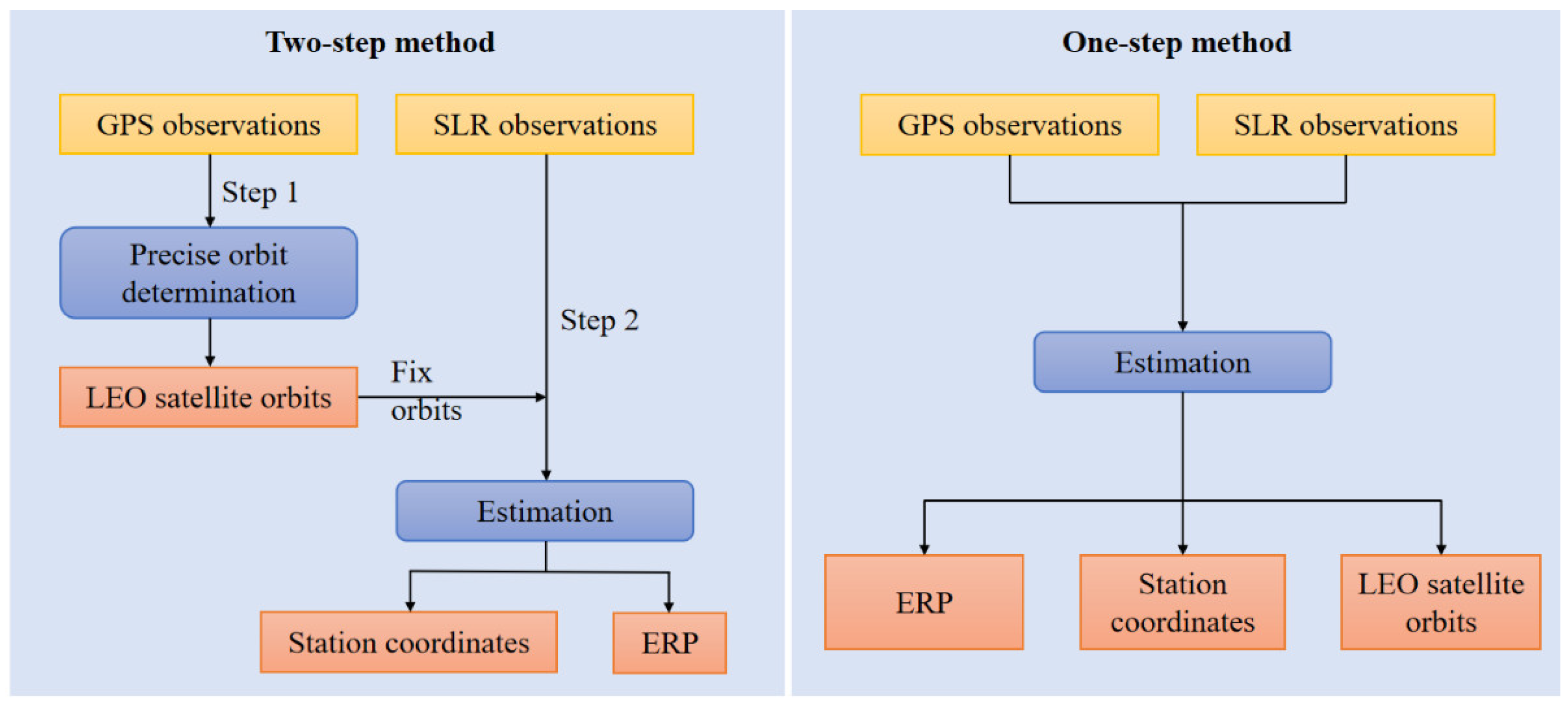
In this study, we adopt two methods to estimate the ERP from the SLR and GPS observations of LEO satellites, namely, the two-step method and one-step method. Figure 1 gives the flowchart of these two methods. In the two-step method, the orbits of the LEO satellites are firstly estimated, using the onboard GPS observations. Here, we choose to independently perform POD for the seven LEO satellites, rather than directly using the external precise orbit products; this is because the external LEO orbit products are generated based on different processing strategies, software platforms and GPS products, and these inconsistencies may introduce additional errors to the final ERP solutions. After the LEO POD processing, we estimate ERP from SLR observations with the LEO orbit fixed.
In the one-step method, the GPS and SLR observations are jointly processed to simultaneously estimate the LEO orbit and ERP in a common least-squares adjustment. The pseudorange, carrier phase observations, and SLR observations are weighted according to the ratio of about 1:15,000:15,000. It should be noted that, in the two-step method, the orbits are only determined based on GPS observations, while in the one-step method, the orbits are calculated using GPS and SLR observations simultaneously. In order to avoid the possible accuracy degradation of the estimated LEO orbit in an orbit arc with a longer length (such as 7 days), in this study we select a 3-day arc length with 2-day overlaps between two adjacent consecutive orbit arcs.
In the LEO POD processing, we use undifferenced ionosphere-free GPS observations with 30-s sampling, and the cutoff elevation angle is set to 1°. The GPS phase center offset (PCO) and phase center variation (PCV) are corrected with igs14.atx [22]. For the LEO satellite antennas, the PCO corrections from ground calibration are employed, while the PCV values are computed using the in-flight calibrated model estimated by the residual method [23,24]. The GPS orbit, clock products, and wide-lane satellite biases products from the Centre National d’Études Spatiales/Collecte Localisation Satellites (CNES/CLS) are used to enable the single-receiver ambiguity fixing [25].
Table 2 summarizes the force model for the POD of the LEO satellites. The N-body gravitation of LEO satellites refers to the gravitational attraction from the sun, the moon, and other planets. The solar radiation pressure of LEO satellites is computed based on the box-wing model with simplified geometric model and panel information. In terms of atmospheric drag, the atmosphere density is computed by the NRLMSISE00 model and a drag scale coefficient is additionally estimated as a piecewise constant parameter to compensate for the mismodeled atmospheric force. The interval of this coefficient varies with the specific satellite, i.e., 90 minutes for GRACE-FO and Swarm satellites, and 100 minutes for Sentinel-3 satellites. Additionally, in order to absorb the unmodeled or mismodeled force errors, a set of cycle-per-revolution empirical accelerations in the along-track and cross-track directions are introduced.
In the step of ERP estimation, we process the available SLR observations that were collected by all the SLR stations. In the SLR observation modelling, the relativity effects, due to the presence of the Earth’s gravitational field, are taken into consideration [28]. We use the zenith delay model proposed by Mendes and Pavlis [31], as well as the mapping function FCULa proposed by Mendes et al. [32], to correct the range delay caused by the troposphere. In addition, the azimuth- and elevation-dependent range correction patterns of laser retroreflector arrays (LRA), derived from Neubert [33] and Montenbruck and Neubert [34], are adopted for the four-prism arrays of GRACE-FO and Swarm, and the seven-prism array of Sentinel-3, respectively.
The estimated parameters that are related to the SLR observations from the LAGEOS and LEO satellites are illustrated in Table 3. We use SLRF2014 (ILRS [35]) to provide a priori reference frame. The no net rotation minimum condition is imposed in order to define the datum. The station coordinates and range biases are estimated as one set of parameters for each three-day solution, with priori constraints of 1 m and 100 m, respectively. It should be noted that in the LAGEOS-involved solutions, only range biases for selected stations are estimated according to the ILRS data handling file. For the ERP, a piecewise linear (PWL) parametrization is applied in order to achieve a better estimation [36]. Since UT1-UTC is correlated with the node of the satellite, it is not possible to independently determine UT1-UTC from any satellite tracking technique, such as SLR or GNSS measurements. Hence, we adopt a similar strategy to that used by the ILRS Analysis Standing Committee, in which UT1-UTC are strongly constrained to the finals2000A.data series published by IERS, and a constraint of 1 m is imposed on the remaining ERPs. In addition, for the LAGEOS-involved solutions, we also estimate the LAGEOS orbit apart from the ERP and station-specific parameters.
All computations are performed on the GNSS+ Research, Application and Teaching (GREAT) software, which is designed and developed at the School of Geodesy and Geomatics of Wuhan University (WHU). The software can support multiple applications, such as multi-technique geodetic parameter estimation, GNSS real-time orbit, and clock determination, PPP-RTK (real-time kinematic) [37], multi-GNSS bias estimation [38], multi-sensor integration navigation, etc.
3. ERP Estimation Based on the Single LEO Satellite
In this section, the quality of the LEO orbit that we calculated is assessed, firstly, by comparison with external products and SLR validation. Then, the influence of LEO orbit improvement on the ERP estimation is assessed. After that, we compare and analyze the ERP solutions based on the different LEO observations, and highlight the differences between these single-LEO solutions.
3.1. Orbit Validation
The capacity of generating high-quality orbit for LEO satellites is a vital prerequisite for the recovery of ERP. Hence, before the ERP estimation, we firstly assess the accuracy of the following two types of LEO orbit solutions that we generated: ambiguity-float solutions and ambiguity-fixed solutions.
Table 4 lists the average root-mean-square (RMS) value of orbit differences, with respect to the external product in the along-track, cross-track and radial components for the ambiguity-float solutions and ambiguity-fixed solutions. Thanks to the additional geometric constraint offered by the ambiguity fixing, the ambiguity-fixed solution shows a smaller RMS value compared to the ambiguity-float solution, and the most distinct improvement is observed in the along-track component. Meanwhile, we can find that GRACE-FO satellites achieve the largest improvement compared to the other missions, and the improvement with respect to the ambiguity-float orbit in the along-track, cross-track and radial components can reach 40%, 13% and 18%, respectively. This can be easily understood by the fact that the GRACE-FO product delivery by JPL is an ambiguity-fixed solution. In the case of Swarm, the benefits of ambiguity fixing are not as evident as they are in the GRACE-FO mission, since the reference orbits are produced with carrier phase ambiguities treated as float values. However, a better consistency to the reference orbits is still visible for the ambiguity-fixed solutions. When referred to Sentinel-3, the consistency with the orbit product is improved for the along-track and radial components in the ambiguity-fixed solution when compared to the ambiguity-float solution. Since the orbit product of Sentinel-3 is based on GPS and Doppler Orbitography by radiopositioning integrated on satellite (DORIS) observations, this result indicates that the ambiguity fixing processing can weaken the inconsistency between the LEO orbit based on different techniques.
Table 5 summarizes the mean bias and standard deviation (STD) of SLR residuals for seven LEO satellites. Here, the SLR validation is performed based on a subset of 12 high-quality core stations (Graz, Greenbelt, Haleakala, Hartebeesthoek, Herstmonceux, Matera, Mt Stromlo, Potsdam, Wettzell (two stations), Yarragadee, and Zimmerwald) [10]. The SLR residuals over ±0.2 m are regarded as outliers and are excluded from the result statistics. As shown in Table 5, an evident reduction of 1–3 mm in STD of SLR residuals of ambiguity-fixed solutions indicates the better orbit accuracy enabled by the ambiguity-fixing processing. These improved orbits will naturally facilitate the estimation of geodetic parameters, such as ERP.
3.2. Impact of Using Ambiguity-Fixed Orbit on the ERP Estimation
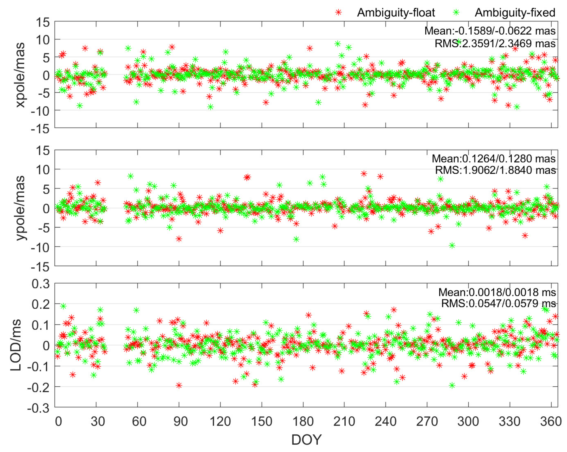
Considering the relationship between the quality of the estimated ERP and LEO orbit accuracy, the contribution of ambiguity-fixed orbit to the ERP estimation is investigated based on the two-step method in this subsection. Taking GRACE-D as an example, Figure 2 typically presents the pole coordinate and LOD differences between the finals2000A.data series and the ERP solutions, based on different orbits. It can be observed that the orbit improvement derived from the ambiguity fixing contributes an evident improvement to the ERP estimation. Compared with the ambiguity-float orbit solution, the ambiguity-fixed orbit solution exhibits a smaller variation, which indicates a better consistency with respect to the finals2000A.data products. With the application of the ambiguity-fixed orbit, the RMS values of X pole and Y pole differences are reduced by 12 uas and 22 uas, respectively, but slight accuracy degradation is observed in LOD.
The benefit of ambiguity fixing is also visible in the coordinates of SLR stations. Table 6 presents the station coordinate differences between SLRF2014 and the different GRACE-D solutions. On average, the interquartile range (IQR) of SLR station coordinates in the east, north and up components are reduced by 18%, 14%, and 13%, respectively, when introducing the ambiguity-fixed orbit. Particularly, the better accuracy is achieved by the core stations, due to the large amount of SLR data they collected. Meanwhile, we can find that the application of the ambiguity-fixed orbit yields a smaller median of core station coordinate differences with respect to the SLRF2014. From the above results, we can conclude that the ERP estimation based on the ambiguity-fixed LEO orbit can obtain a better result. Therefore, all LEO-involved ERP solutions hereafter are performed based on the ambiguity-fixed orbit.
3.3. ERP Estimation with Different LEO Satellites
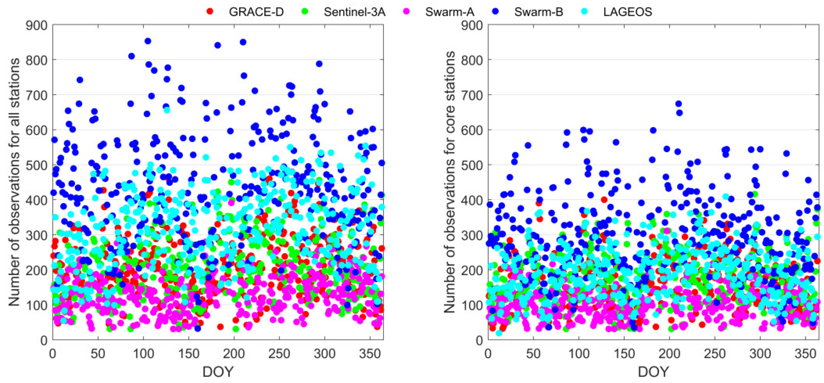
Figure 3 typically presents the number of SLR observations (normal points, NPs) of each 3-day solution for GRACE-D, Sentinel-3A, Swarm-A, Swarm-B, and LAGEOS satellites. An evident difference between LEO and LAGEOS satellites can be noted. In general, the average number of SLR observations used for a 3-day solution is 213, 204, 129, 437, and 317 for GRACE-D, Sentinel-3A, Swarm-A, Swarm-B and LAGEOS, respectively. The largest number of SLR observations is achieved by Swarm-B, which is even over three times more than that of Swarm-A. The observation number of most LEO cannot reach a similar level to that of LAGEOS, because there are two LAGEOS satellites and LAGEOS are calibration satellites for SLR stations, hence most stations track them. In addition, we can see that the core stations contribute to almost 70% of the SLR observations for LEO and LAGEOS satellites.
Table 7 presents the statistical data of ERP based on SLR observations to seven LEO satellite ambiguity-fixed orbits, respectively. The LAGEOS-based solution is also listed here to provide a reference. In the case of a single-LEO solution, the estimated ERP become more sensitive to the number of SLR observations, since only one LEO satellite is used. We can find that the quality of ERP exhibits a strong dependence on the observation numbers. Among the LEO-based solutions, the Swarm-B solution exhibits the best consistency with the IERS product, thanks to its obviously largest number of available observations, and the RMS value for X pole, Y pole and LOD is 1.9286 ms, 1.6634 ms and 0.0673 ms, respectively. It should be noted that, though the nearly comparable amount of SLR observations is achieved for GRACE-FO and Sentinel-3 satellites, the Sentinel-3 solution shows an evidently worse ERP result than that of GRACE-FO solutions. The main reason for this phenomenon is that the specific sun-synchronous orbit of Sentinel-3, with the orbital inclination of 98.6±, results in a low sensitivity for polar motion [41]. On the other hand, the relatively lower orbit accuracy of Sentinel-3 also accounts for their degraded ERP result (see Table 5). It can be seen that the accuracy of single-LEO solutions is not comparable to that of the LAGEOS solution, even for the Swarm-B solution. The superior performance of the LAGEOS solution is resulted from their simple satellite structure, the uncomplicated force model, and enough observations.
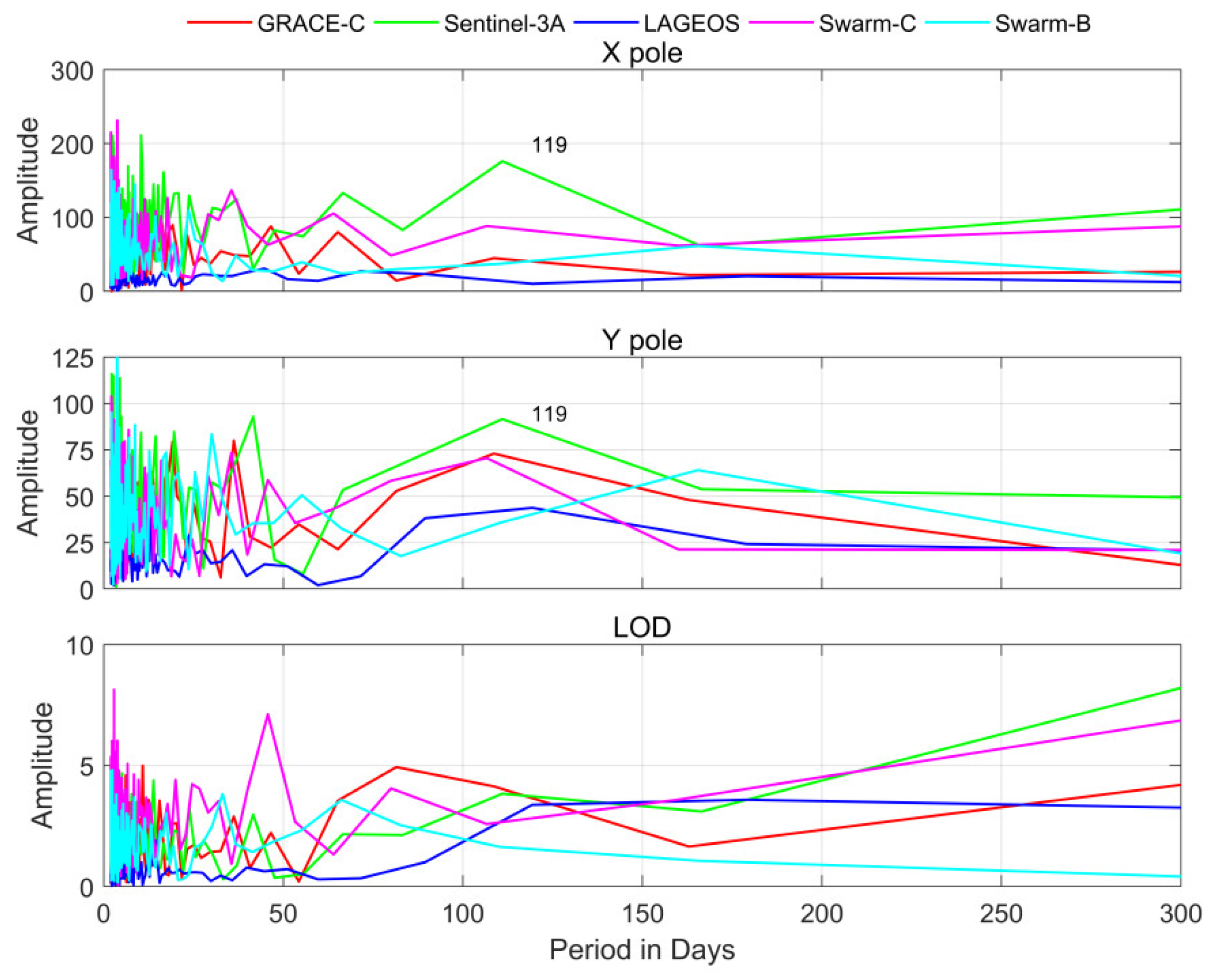
Figure 4 typically gives the spectral analysis results for four single-LEO solutions and the LAGEOS solution. It can be seen that the LEO solutions apparently have more noisy signals with the period up to 50 days than the LAGEOS solution. No evident semiannual signal is visible in all the solutions. However, a distinct signal, with a 119-day period in the pole coordinates, can be observed in the Sentinel-3A solution. This signal may be related with the perigee revolution of 122 days for the Sentinel-3 satellite.
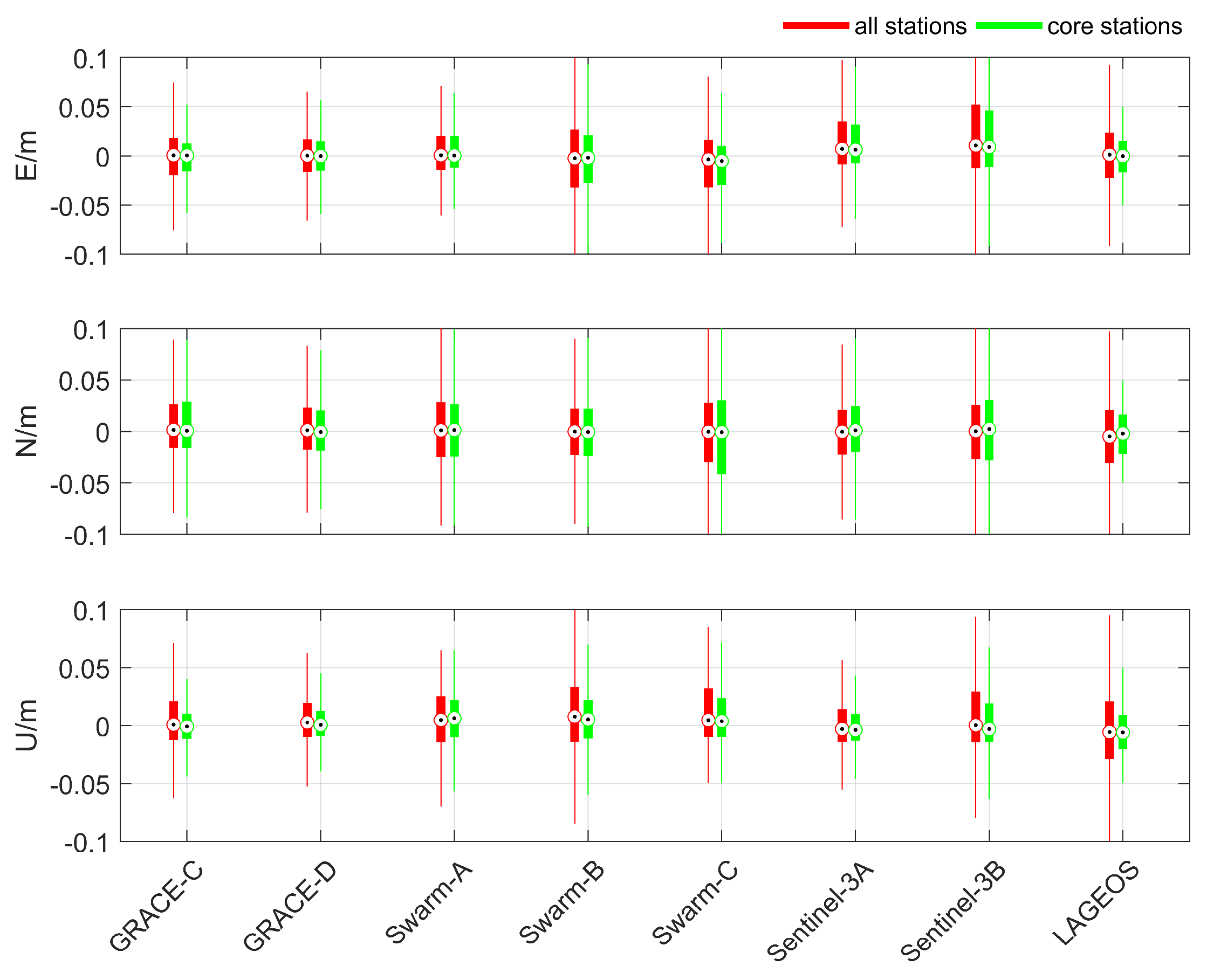
Figure 5 gives the differences of the estimated station coordinates w.r.t SLRF2014 for the different satellite solutions, and summarized data are shown in Table 8. For all the LEO solutions, the positioning of all the SLR stations obtains the accuracy at the level of 20 mm–30 mm. While for the core stations, the accuracy level can reach about 10 mm–20 mm. Although there is the largest number of available observations for Swarm-B, the Swarm-B solution is inferior, with an IQR of 29 mm, 23 mm and 24 mm in three components for all the stations, which is probably due to the relatively poor precision of the Swarm-B orbits (see Table 5). Among these LEO satellite solutions, the GRACE-C and GRACE-D solutions can obtain better results than other solutions, with an IQR of about 15–20 mm in the E, N, U components for all the stations, thanks to their high-accuracy ambiguity-fixed orbit. These results illustrate that the accuracy of station coordinates are more sensitive to the quality of the LEO orbit, under the condition that enough SLR observations to the LEO satellite can be obtained.
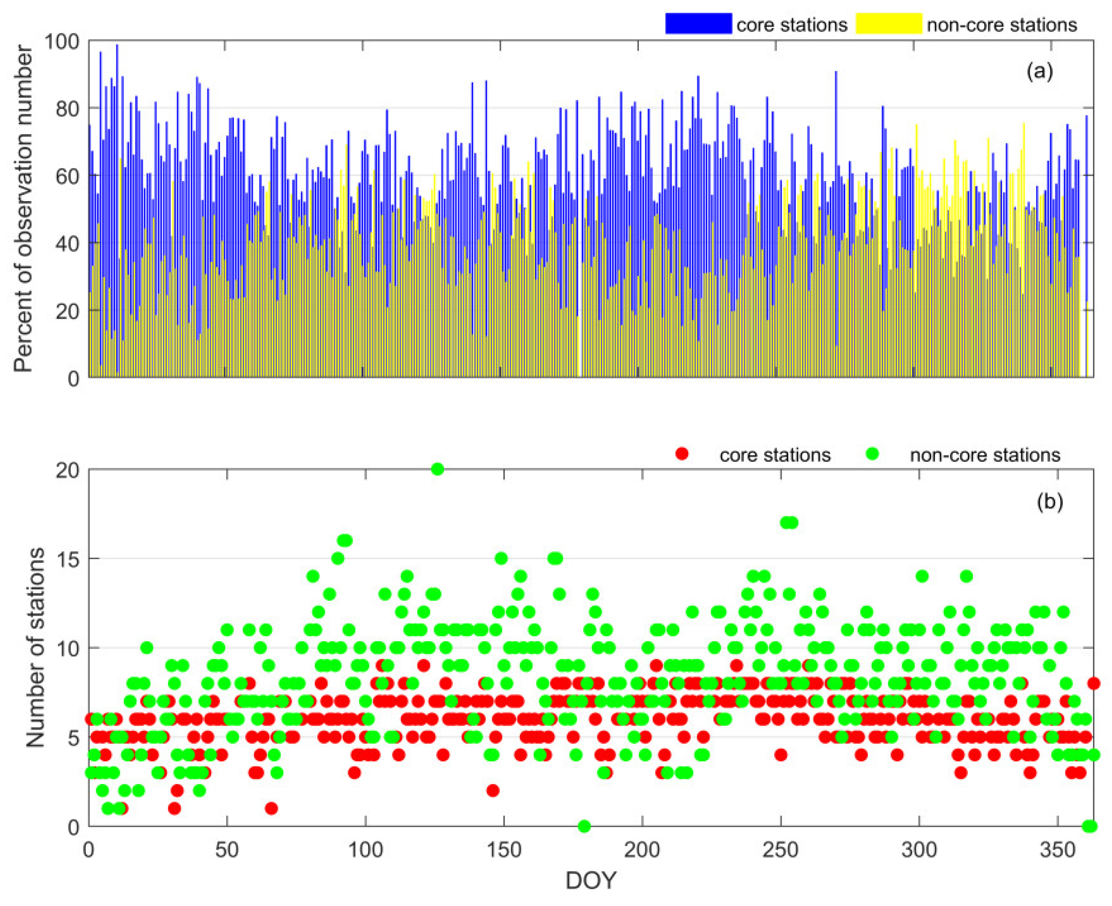
As shown in Table 8, the LAGEOS solution achieves a station coordinate with worse accuracy than some single-LEO solutions, such as GRACE-C, GRACE-D and Sentinel-3A solutions, when considering all the SLR stations. In order to explain this phenomenon, here we give Figure 6, which shows the percentage of observations from core stations and non-core stations for LAGEOS satellites, and the number of core stations and non-core stations. We can see that the non-core stations account for a large part of the stations tracking LAGEOS, but only contribute to about 30% of SLR observations to LAGEOS. The small amount of observations for non-core stations weaken the solution strength for the station coordinates, and lead to a degraded positioning accuracy for non-core stations. This may explain the larger average RMS values with an IQR of nearly 25 mm for the E, N, and U components for all the stations. For the core stations, LAGEOS and some LEO solutions can achieve a comparable positioning accuracy, and the GRACE-C and GRACE-D solutions even present a smaller RMS value in the up component, with an IQR decrease of nearly 4 mm. These analyses suggest that it is tenable to achieve a desirable station coordinate result based on the LEO orbit of high accuracy.
4. ERP Estimation Based on the Combination of Multiple LEO Satellites
In this section, we focus on the ERP estimation using the onboard data from multiple LEO satellites. The quality of ERP solutions, based on the different combinations of LEO satellites, is firstly investigated. Then, we perform a combined solution with LAGEOS and LEO satellites in order to explore the contribution of LEO satellites. Finally, a comparison between the one-step solution and two-step solution is presented.
4.1. Impact of LEO Number on the ERP Estimation
In order to investigate the impact of LEO number on the ERP estimation, three combination solutions with 3-, 5- and 7-LEO satellites have been performed. The design of these schemes is on the basis of maximizing the diversity of orbit type, which is beneficial for eliminating the LEO-related orbit signals in ERP estimation. The 3-LEO scheme includes GRACE-C, Swarm-A, and Sentinel-3A. The 5-LEO scheme indicates the solution generated using GRACE-C, GRACE-D, Swarm-A, Swarm-B, and Sentinel-3A satellites. The 7-LEO scheme is with all the LEO satellites mentioned in Section 2, which maximizes the number of LEO observations and further strengthens the observation geometry.
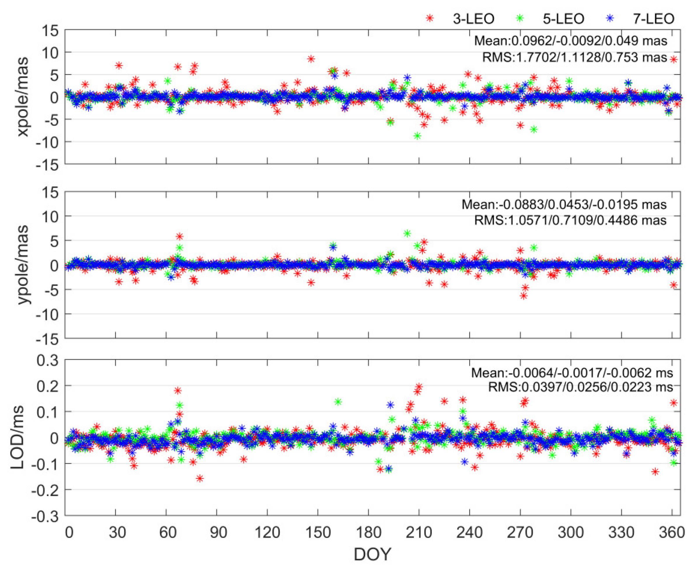
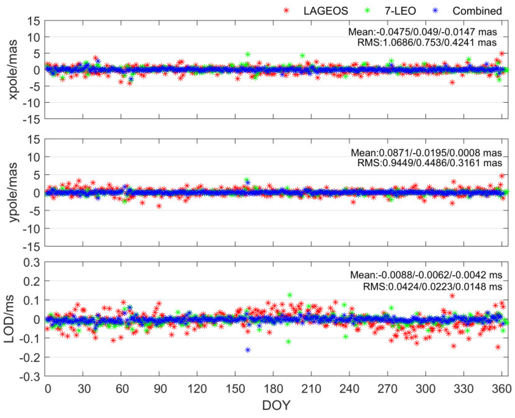
The results from the 3-LEO, 5-LEO and 7-LEO solutions are illustrated in Figure 7. Figure 7 shows that the scatter distributions of the 7-LEO solution are much denser near the zero line than those of the 3-LEO and 5-LEO solutions. The ERP RMSs of the 3-LEO solution are the largest, and the best result occurs in the 7-LEO solution with the RMSs of 0.7530 ms, 0.4486 ms and 0.0223 ms for X pole, Y pole and LOD, respectively. It indicates that more LEO satellites included in the estimation lead to a smaller ERP RMS. This improvement can be attributed to the significant increase in SLR observations, and the enhanced observation geometry with more LEO satellites. Moreover, the 7-LEO solution performs better than the LAGEOS solution (see Table 7) for ERP estimation, which indicates that for the ERP estimation under the short arc condition, the multiple-LEO solution can reach a similar or even better accuracy compared with the LAGEOS solution.
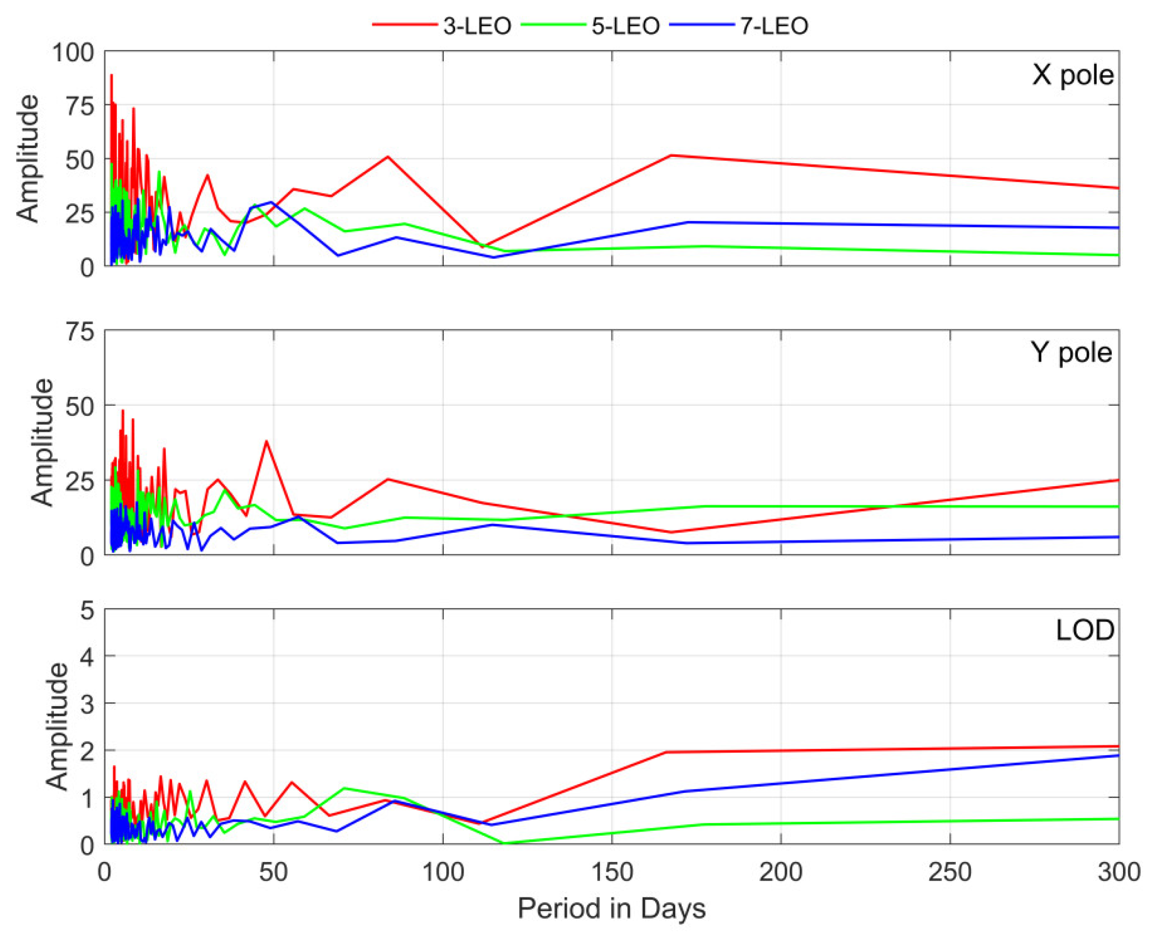
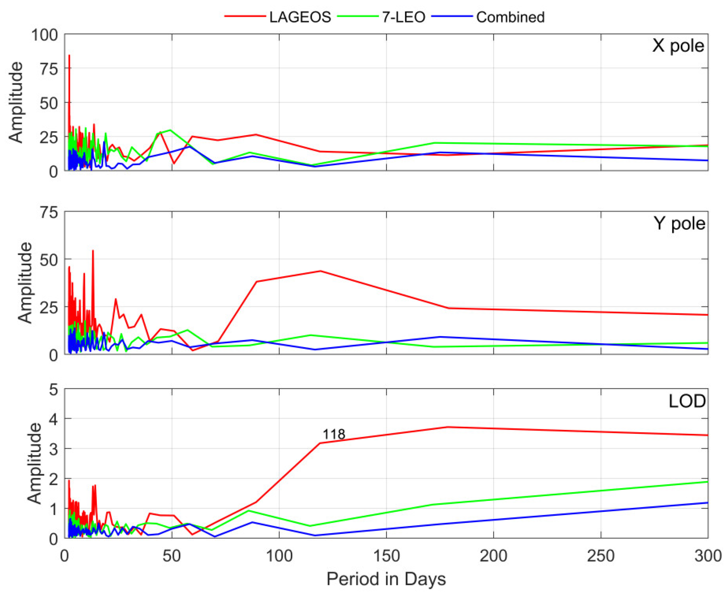
Figure 8 gives the spectral analysis for the 3-LEO, 5-LEO and 7-LEO solutions. It can be clearly observed that the 119-day period for Sentinel-3A, mentioned in Section 3.3, is eliminated in the 3-LEO solution, which suggests that the ERP estimation with multiple LEO satellites can mitigate the orbit-related signal of single LEO in ERP solutions. Moreover, the amplitude of the 5-LEO solution is smaller than that of the 3-LEO solution for X pole, Y pole, and LOD. This indicates that the inclusion of Swarm-B and GRACE-D improves the orbit diversification, which can further improve the ERP solution. Additionally, the 7-LEO solution obtains the smallest amplitude within the period less than 120 days.
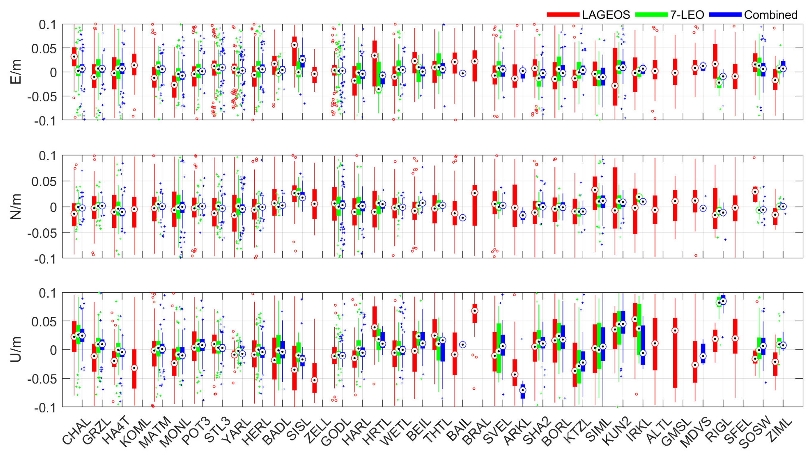
Figure 9 shows the differences in all the stations’ coordinates w.r.t SLRF2014 for the 3-LEO, 5-LEO, and 7-LEO solutions. The corresponding statistics are severally listed in Table 9. With more LEO satellites included in, more observations can be used for estimating station coordinates. For core station solutions, a notable improvement can be seen in the north component. Compared with the 3-LEO solution, the 7-LEO solution improves by 32% in the north component. For the non-core stations, we can find that the combination of more LEO satellites can lead to an obvious improvement in all three components for non-core stations. The best results for non-core stations are in the 7-LEO solution, with IQRs of 19.6 mm, 13.6 mm, and 25.6 mm in the east, north, and up component, respectively. This is because more LEO satellites bring more observations and strengthen the observation geometry, which is especially vital for the estimation of these non-core stations with less observations. In addition, there are some stations, such as SVEL and BEIL, whose coordinates are unavailable in the 3-LEO solution, due to the lack of observations. However, we can get a relatively reliable coordinate solution for such stations in the 5-LEO and 7-LEO solutions. This further confirms the advantage of the combination of LEO satellites.
4.2. Combination of LEO Satellite and LAGEOS
The routine ERP product from ILRS is majorly based on LAGEOS. Hence, the investigation of the contribution of LEO satellites and LAGEOS combination to ERP estimation is especially meaningful. Figure 10 shows the ERP differences w.r.t the finals2000A.data series of the LAGEOS solution, the 7-LEO solution, and the combined solutions. The combined solution characterized by more concentrated blue dots reflects that the stability of the ERP solution is notably improved. In contrast to the LAGEOS solution, the combined solution shows RMS reductions of 0.644 ms, 0.629 ms and 0.028 ms for X pole, Y pole and LOD, respectively, since the involvement of seven LEO satellites offers a large number of observations. Besides, from the spectrum in Figure 11, it can be seen that the correlations between the LOD and LAGEOS satellite orbital parameters are weakened when LEO satellites are included. The 118-day period signal in LOD, which is related to the 112.5-day eclipsing period of LAGEOS-2, is visibly mitigated in the combination solution. When compared with the 7-LEO solution, the combination of LAGEOS and seven LEO satellites also attains a superior result, with a distinct decrease in the RMS of ERP.
Figure 12 depicts the differences in all the estimated SLR station coordinates w.r.t. SLRF2014, and the statistical data are presented in Table 10. For all the stations, the combination of seven LEO satellites and LAGEOS satellites can obtain a superior coordinate result, with an IQR below 10 mm in the east and north components, which improves notably when compared with the LAGEOS solution and 7-LEO solution. It is visible that the estimated coordinates of the core stations are further improved when the LEO data are included. The results for the core station with the combination of LEO satellites and LAGEOS can reach the accuracy level below 10 mm in all three components. The combination solution is improved by 7 mm, 3 mm, and 3 mm compared to the 7-LEO solution.
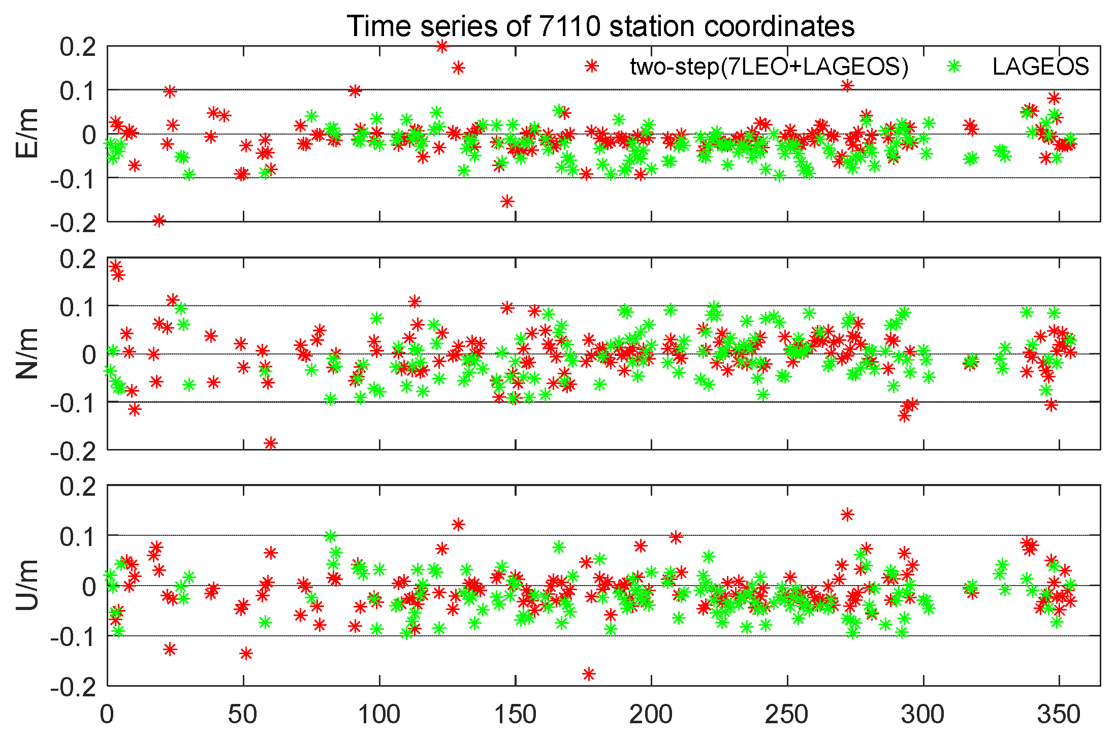
Additionally, the LEO observations can serve as a supplement in the case where the high-quality LAGEOS data are missing. Figure 13 gives the time series of 7110 station coordinates. It can be observed that the coordinate solution of the station is unavailable from DOY 10 to DOY 20, and from DOY 40 to DOY 50 in the LAGEOS solution, due to the lack of observations. When the LEO data are used, the station coordinates’ time series can be more continues, with denser red dots. It indicates that the combination of LEO satellites and LAGEOS can maximize the number of solved stations and strengthen the continuity of the station coordinate solutions.
4.3. Comparison of One-Step and Two-Step Methods
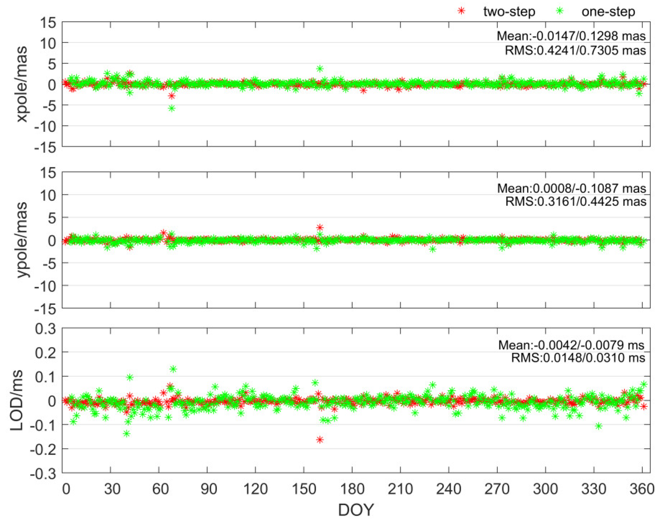
Based on the observations of LAGEOS and seven LEO satellites, the one-step method is implemented and compared with the two-step method. Figure 14 shows the comparison of the ERP results derived from the two-step and one-step methods. When the one-step method is implemented, with the combination of seven LEO satellites and LAGEOS, an evident accuracy degradation is visible in the ERP result. Especially for the LOD parameter, a factor of 2.0 increase in RMS is observed. The similar degradation in simultaneously estimating the orbit and ERP also occurs in the ERP series derived from SLR observations to GNSS satellites, as reported by Sośnica et al. [42]. This is possibly because of the introduction of orbit parameters. In the one-step solution, the orbit parameters of LEO satellites, such as the initial positions and velocities of LEO satellites, atmospheric drag scale parameter and empirical accelerations, have to be additionally estimated, which substantially increases the degree of freedom and weakens the stability of the solution.
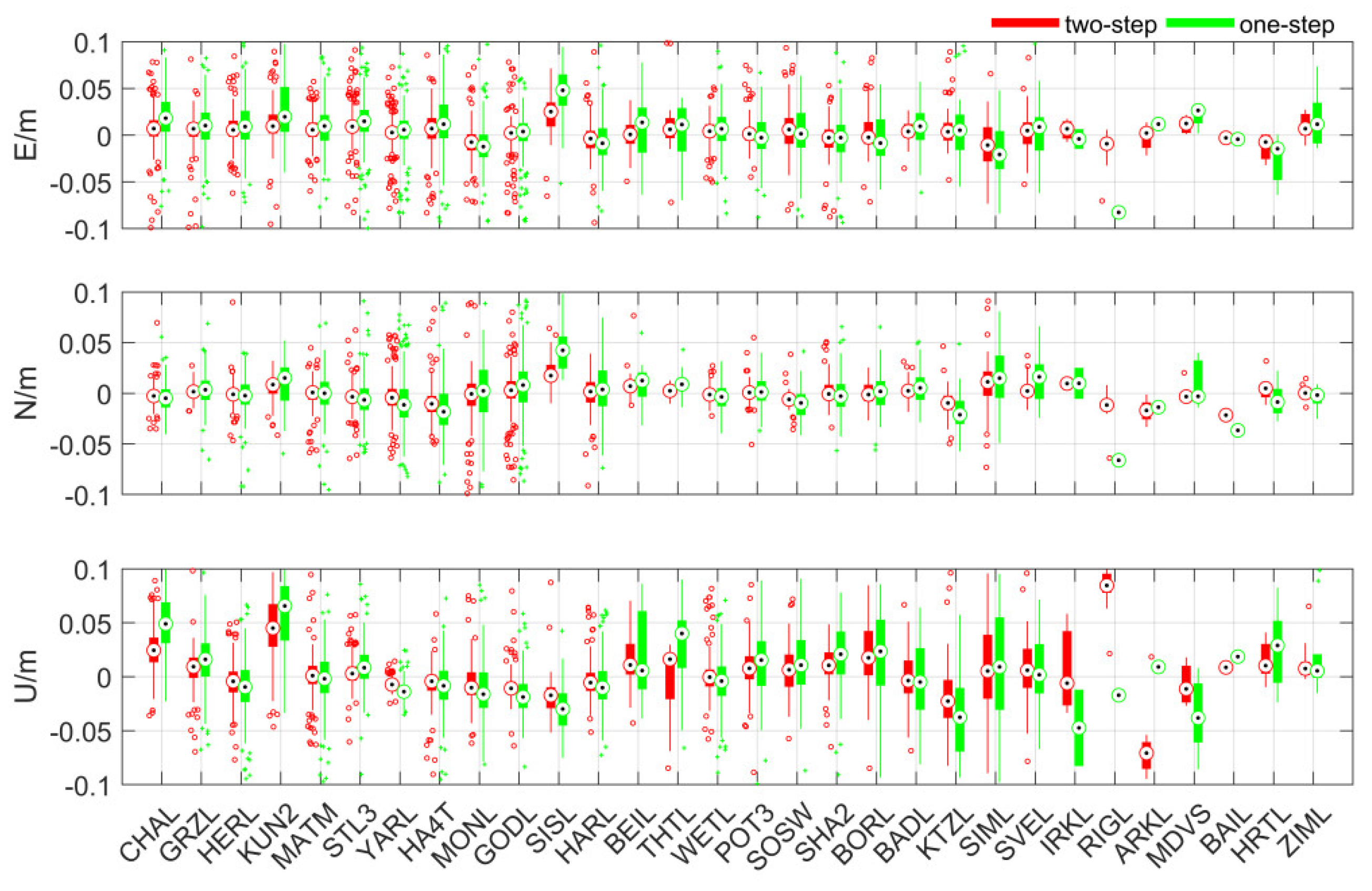
Figure 15 presents the differences of all the estimated SLR station coordinates w.r.t. SLRF2014 for the two-step method and one-step method. Statistical data are shown in Table 11. When the one-step method is compared with the two-step method, the results for all the stations become worse, with an IQR of 15 mm, 14 mm, and 20 mm in the east, north and up components, respectively. Such degradation possibly occurs because the orbit deficiencies are propagated into the obtained station coordinate, while the LEO orbit and station coordinates are estimated simultaneously in the one-step method. Additionally, in one-step method the GPS observations are also processed, in which the SLR results are possibly affected by errors in the GPS data and data processing.
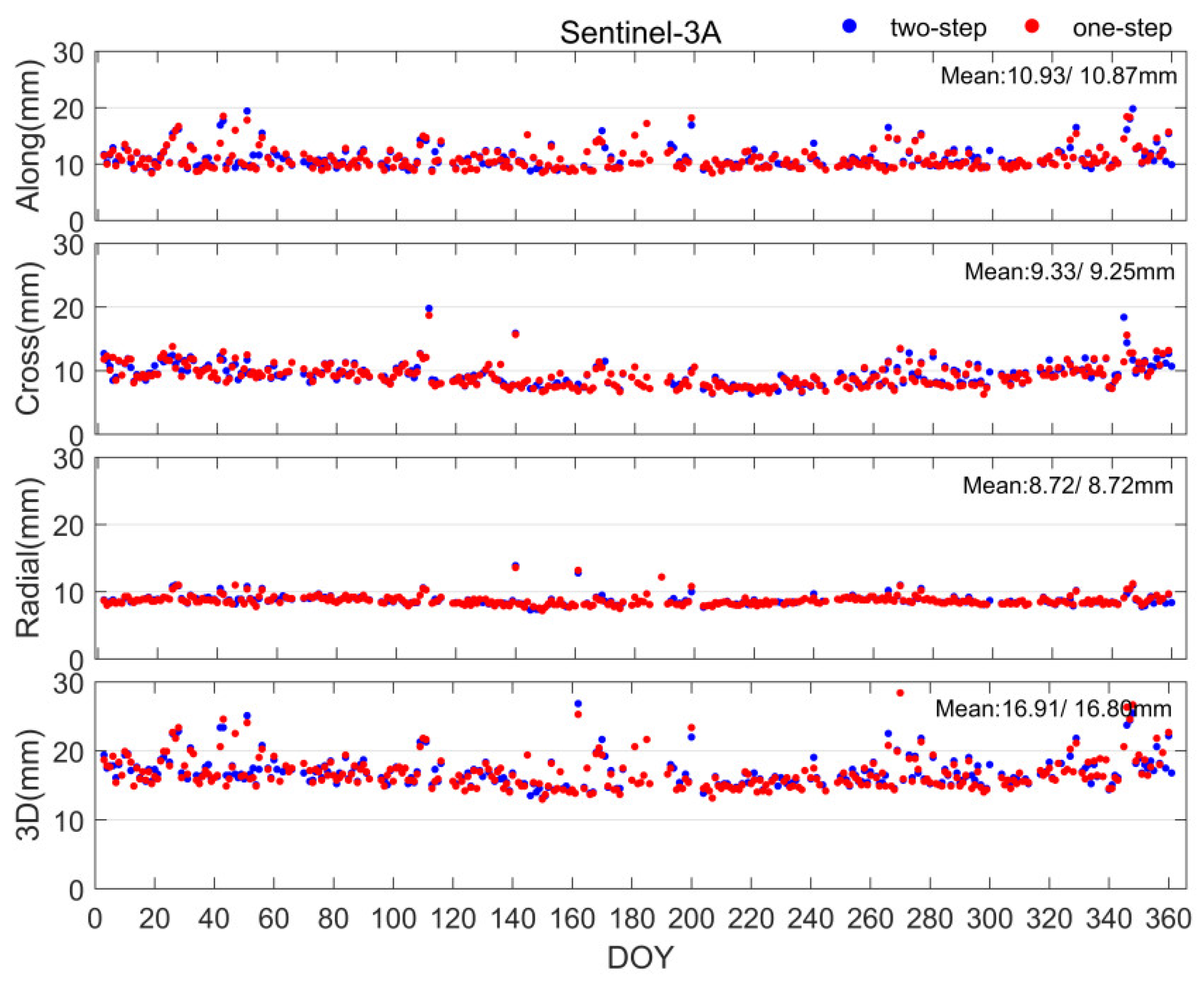
In addition, we also assess the quality of the LEO orbit derived from the two-step and one-step methods. Here, we take Sentinel-3A as an example, since the orbit product of Sentinel-3 from CNES is based on DORIS and GPS observations. Figure 16 shows the average RMS of orbit difference with respect to the orbit product of Sentinel-3A. This figure shows that, compared with the two-step solution, the orbit of the one-step solution can achieve a slight accuracy improvement at the level of sub-millimeter. A similar benefit is also reported by Guo et al. [43], Jäggi et al. [44], and Wirnsberger et al. [45]. Such improvement can be attributed to the increased observations and strengthened observation geometry that benefit from additional SLR observations in the one-step method. It demonstrates that the inclusion of SLR observations can eliminate the inter-technique inconsistency between the GPS-only orbit and GPS–DORIS-based orbit product to some extent.
5. Discussion
This paper is devoted to discussing the contribution of LEO satellites to ERP estimation. The SLR observations to seven LEO satellites from three different missions, including Sentinel-3, Swarm, and GRACE-FO, are processed in this study. With the proposed single-receiver phase ambiguity resolution method in [39], the ambiguity-fixed orbit is used for decreasing the impact of possible orbit error in the ambiguity-float orbit for ERP estimation. We find that the single-LEO ERP solution cannot reach the comparable accuracy level of the LAGEOS solution, even if the ambiguity-fixed orbit is used. The same phenomenon also occurs in [9]. This may be due to the limited observations for single-LEO satellites, or the LEO satellite orbit-related errors conveyed into the ERP solution. The station coordinate derived from the single-LEO solutions can reach the similar accuracy of a few centimeters with that in [20]. For the estimated core station coordinates, the solution based on some LEO satellites, such as GRACE-C and GRACE-D, is comparable to that based on LAGEOS satellites. This phenomenon confirms the potential of LEO satellites in geodetic parameter estimation to some extent.
Rather than just focus on the single-LEO satellite, the combination of multiple-LEO satellites for ERP estimation is highlighted in our study. By increasing the LEO number in the processing, a notable improvement can be observed in the ERP solution. With seven LEO satellites included, a better ERP result than that based on LAGEOS in [46] is obtained. Moreover, the combination of multiple LEO satellites is especially of benefit for weakening the LEO orbit-related signal in single-LEO solutions. Furthermore, the combination of seven LEO satellites and LAGEOS satellites can reach the best result, with the smallest RMS for ERP. Such combination offers a large number of observations and maximizes the diversity of the orbit type, which is especially beneficial for estimating ERP and obtaining more reliable estimated station coordinates. Our result indicates that this method exhibits a great potential to be a strong supplement, even an alternative to the current SLR-based reference frame realization only based on LAGEOS and Etalon satellites.
6. Conclusions
A large amount of SLR observations to LEO satellites offer an opportunity for investigating the potential of LEO satellites in ERP estimation. In this study, we are devoted to recovering ERP using SLR and GPS observations from seven LEO satellites. We evaluate the impact of the LEO orbit improvement on ERP estimation, and compare the quality of the ERP solution based on different LEO satellites. The main focus is on the different performance of the single-LEO solution, and the benefit of the combination of LEO satellites. In addition, we also investigate the feasibility of the simultaneous estimation of LEO orbits and ERP, which is named the one-step method in this study.
The contribution of the ambiguity-fixed orbit for ERP estimation is firstly confirmed. Compared to the ambiguity-float solution, an RMS decrease of 12 uas and 22 uas for X pole and Y pole is obtained in the ambiguity-fixed solution. Based on the ERP series of different single-LEO solutions, we find that the single-LEO ERP solution cannot reach the comparable accuracy level of the LAGEOS solution, due to the limited SLR observations or the orbit modeling deficiencies. Meanwhile, a 119-day period signal is observed in the spectrum of the Sentinel-3 solution, which is closely related to the perigee revolution of the Sentienl-3 satellite. For the SLR stations, it can be seen that the station coordinates at the accuracy level of 2–3 cm is achievable while only using one LEO satellite. For the core stations, some single-LEO solutions can achieve a comparable positioning accuracy to the LAGEOS solution. In particular, the GRACE-C and GRACE-D solutions present an improvement of 4 mm in the up component when compared to the LAGEOS solution.
Then, multiple LEO solutions with different numbers of LEO satellites are explored, with three schemes of the 3-LEO, 5-LEO and 7-LEO. The best ERP estimation result is achieved by the 7-LEO solution, thanks to a large number of observations and the enhanced observation geometry. Compared to the 3-LEO solution, the accuracy of X pole, Y pole and LOD for the 7-LEO solution is improved by 57.5%, 57.6% and 43.8%, respectively. Moreover, with more satellites included, the correlation between orbit parameters and ERP is significantly reduced. It can be seen that the 119-day signal in the Sentinel-3A solution is weakened in the multiple-LEO satellite solutions. For the station coordinates, more observations from multiple-LEO satellites contribute to a more accurate and stable positioning solution, especially for the non-core station, which usually owns few observations in the single-LEO solution or LAGEOS solution. It can be seen that when the number of LEO satellites increases from three to seven, the accuracy of the non-core station coordinates is improved by 13.7%, 27.3% and 16.2% in the east, north and up components, respectively.
We also jointly processed the data of LAGEOS and seven LEO satellites for ERP estimation, and this combination scheme attains an RMS reduction of 0.644 ms, 0.629 ms and 0.028 ms for X pole, Y pole and LOD, compared to the LAGEOS solution. Besides, the results for the core station can reach the accuracy level below 10 mm in the east, north and up components. In addition, we discuss the possibility of simultaneously estimating LEO orbits and ERP using GPS and SLR data. A degraded ERP and the station coordinate result is observed when the integrated processing is performed, which may be attributed to the weakened solution strength caused by introducing a large number of orbit parameters. However, it is desirable to obtain a sub-millimeter improvement for LEO satellite orbit estimation from the one-step method, thanks to the combination of GPS and SLR observations in the precise orbit determination process.
Author Contributions
Conceptualization, X.L. and H.Z.; methodology, X.L. and H.Z.; software, X.L.; validation, H.Z. and K.Z.; formal analysis, H.Z.; investigation, H.Z. and K.Z.; resources, Y.Y. and Y.Q.; data curation, H.Z.; writing—original draft preparation, H.Z.; writing—review and editing, K.Z. and H.Z.; visualization, H.Z.; supervision, W.Z.; project administration, X.L.; funding acquisition, X.L. All authors have read and agreed to the published version of the manuscript.
Funding
This research was funded by the National Natural Science Foundation of China (grant 41774030, grant 41974027 and grant 41974029), the Hubei Province Natural Science Foundation of China (grant 2020CFA002), the frontier project of basic application from Wuhan Science and Technology Bureau (grant 2019010701011395), and the Sino-German mobility programme (grant No. M-0054).
Acknowledgments
We are grateful to the International GNSS Service (IGS) for providing the precise orbit, clock and correction products of GPS satellites at ftp://cddis.gsfc.nasa.gov (accessed on 1 June 2021) for free. The ILRS is acknowledged for providing SLR observations of LEO and LAGEOS satellites. The data onboard GRACE-FO, Swarm, and Sentinel-3 are publicly available from ftp://isdcftp.gfz-potsdam.de (accessed on 1 June 2021), ftp://swarm-diss.eo.esa.int (accessed on 1 June 2021) and https://scihub.copernicus.eu/gnss (accessed on 1 June 2021) respectively. The numerical calculations in this study have been done on the supercomputing system in the Supercomputing Center of Wuhan University.
Conflicts of Interest
The authors declare no conflict of interest.
References
- Teunissen, P.; Montenbruck, O. Springer Handbook of Global Navigation Satellite Systems; Springer International Publishing: Berlin/Heidelberg, Germany, 2017. [Google Scholar]
- Smith, D.E.; Turcotte, D.L. Variations in the orientation of the earth, In Contributions of Space Geodesy to Geodynamics: Earth Dynamics; American Geophysical Union: Washington, DC, USA, 1993; Volume 24, pp. 1–54. [Google Scholar]
- Kalarus, M.; Schuh, R.; Kosek, R.; Akyilmaz, R.; Bizouard, R.; Gambis, R.; Gross, R.; Jovanovic, R.; Kumakshev, R.; Kutterer, R. Achievements of the earth orientation parameters prediction comparison campaign. J. Geod. 2010, 84, 587–596. [Google Scholar] [CrossRef]
- Raposopulido, V.; Kayikci, E.T.; Heinkelmann, R.; Nilsson, T.; Karbon, M.; Soja, B.; Lu, C.; Moradiaz, J.; Schuh, H. Impact of Celestial Datum Definition on EOP Estimation and CRF Orientation in the Global VLBI Session IYA09; Springer: Berlin/Heidelberg, Germany, 2010; Volume 30, pp. 297–311. [Google Scholar]
- Gross, R.S. Earth rotation variations–long period-3.09. In Treatise on Geophysics, 2nd ed.; Elsevier: Amsterdam, The Netherlands, 2015; pp. 215–261. [Google Scholar]
- Dehant, V.; Mathews, P.M. Earth Rotation Variations. In Treatise on Geophysics, 2nd ed.; Elsevier: Amsterdam, The Netherlands, 2015; pp. 263–305. [Google Scholar]
- Sonica, K.; Zajdel, R.; Bury, G.; Strugarek, D.; Prange, L. Geocenter coordinates and Earth rotation parameters from GPS, GLONASS, Galileo, and the combined GPS+GLONASS+Galileo solutions. In Proceedings of the EGU General Assembly 2020, online, 4–8 May 2020. [Google Scholar]
- Pearlman, M.R.; Noll, C.E.; Pavlis, E.C.; Lemoine, F.G.; Combrink, L.; Degnan, J.D.; Kirchner, G.; Schreiber, U. The ILRS: Approaching 20 years and planning for the future. J. Geod. 2019, 93, 2161–2180. [Google Scholar] [CrossRef]
- Strugarek, D.; Sonica, K.; Arnold, D.; Jggi, A.; Drodewski, M. Determination of global geodetic parameters using satellite laser ranging measurements to sentinel-3 satellites. Remote Sens. 2019, 93, 2282. [Google Scholar] [CrossRef] [Green Version]
- Daniel, A.; Oliver, M.; Stefan, H.; Krzysztof, S. Satellite laser ranging to low Earth orbiters: Orbit and network validation. J. Geod. 2019, 93, 2315–2334. [Google Scholar]
- Cheng, M.K.; Shum, C.K.; Eanes, R.J.; Schutz, B.E.; Tapley, B.D. Long-period perturbations in starlette orbit and tide solution. J. Geophys. Res. Solid Earth 1990, 95, 8723–8736. [Google Scholar] [CrossRef]
- Hashimoto, H.; Nakamura, S.; Shirai, H.; Sengoku, A.; Otsubo, T. Japanese geodetic satellite ajisai: Development, observation and scientific contributions to geodesy. J. Geod. Soc. Jpn. 2012, 58, 9–25. [Google Scholar]
- Sosnica, K.; Jaeggi, A.; Thaller, D.; Beutler, G.; Dach, R. Contribution of starlette, stella, and ajisai to the slr-derived global reference frame. J. Geod. 2014, 88, 789–804. [Google Scholar] [CrossRef] [Green Version]
- Rutkowska, M.; Jagoda, M. Estimation of the elastic earth parameters using slr data for the low satellites STARLETTE and STELLA. Acta Geophys. 2012, 60, 1213–1223. [Google Scholar] [CrossRef]
- Lejba, P.; Schillak, S. Determination of station positions and velocities from laser ranging observations to Ajisai, Starlette and Stella satellites. Adv. Space Res. 2011, 47, 654–662. [Google Scholar] [CrossRef]
- Tapley, B.D.; Bettadpur, S.; Ries, J.C.; Thompson, P.F.; Watkins, M.M. GRACE measurements of mass variability in the earth system. Science 2004, 305, 503–505. [Google Scholar] [CrossRef] [PubMed] [Green Version]
- Kang, Z.; Bettadpur, S.; Nagel, P.; Save, H.; Pie, N. Grace-fo precise orbit determination and gravity recovery. J. Geod. 2020, 94, 1–17. [Google Scholar] [CrossRef]
- Montenbruck, O.; Hackel, S.; Jaggi, A. Precise orbit determination of the sentinel-3a altimetry satellite using ambiguity-fixed gps carrier phase observations. J. Geod. 2018, 92, 711–726. [Google Scholar] [CrossRef] [Green Version]
- Montenbruck, O.; Stefan, H.; Jose, V.D.I.; Daniel, A. Reduced dynamic and kinematic precise orbit determination for the swarm mission from 4years of gps tracking. GPS Solut. 2018, 22, 1–11. [Google Scholar] [CrossRef]
- Guo, J.; Wang, Y.; Shen, Y.; Liu, X.; Sun, Y.; Kong, Q. Estimation of slr station coordinates by means of slr measurements to kinematic orbit of leo satellites. Earth Planets Space 2018, 70, 1–11. [Google Scholar] [CrossRef] [Green Version]
- Bloßfeld, M.; Zeitlhöfler, J.; Rudenko, S.; Dettmering, D. Observation-based attitude realization for accurate jason satellite orbits and its impact on geodetic and altimetry results. Remote Sens. 2020, 12, 682. [Google Scholar] [CrossRef] [Green Version]
- Rebischung, P.; Schmid, R.; Herring, T. Upcoming Switch to IGS14/igs14.atx. IGSMAIL-7399. Available online: https://igscb.jpl.nasa.gov/pipermail/igsmail/2016/008589.html (accessed on 21 December 2016).
- Haines, B.; Bar-Sever, Y.; Bertiger, W.; Desai, S.; Willis, P. One-centimeter orbit determination for Jason-1: New GPS-based strategies. Mar. Geod. 2004, 27, 299–318. [Google Scholar] [CrossRef]
- Lu, C.; Zhang, Q.; Zhang, K.; Zhu, Y.; Zhang, W. Improving leo precise orbit determination with bds pcv calibration. GPS Solut. 2019, 23, 1–13. [Google Scholar] [CrossRef]
- Loyer, S.; Perosanz, F.; Mercier, F.; Capdeville, H.; Marty, J.C. Zero difference GPS ambiguity resolution at CNES-CLS IGS analysis center. J. Geod. 2012, 86, 991–1003. [Google Scholar] [CrossRef]
- Standish, E.M. JPL Planetary and Lunar Ephemerides, DE405/LE405. Interoffice Memorandum: JPL IOM 312.F-98-048, 1998 August 26. Available online: ftp://ssd.jpl.nasa.gov/pub/eph/planets/ioms/de405.iom.pdf (accessed on 1 June 2021).
- Lyard, F.; Lefevre, F.; Letellier, T.; Francis, O. Modelling the global ocean tides: Modern insights from FES2004. Ocean. Dyn. 2006, 56, 394–415. [Google Scholar] [CrossRef]
- IERS. IERS Conventions 2010: IERS Technical Note 36; Petit, G., Luzum, B., Eds.; Verlag des Bundesamts für Kartographie und Geodäsie: Frankfurt am Main, Germany, 2011. [Google Scholar]
- Montenbruck, O.; Gill, E. Satellite Orbits; Springer: Berlin/Heidelberg, Germany, 2005. [Google Scholar]
- Picone, J.M.; Hedin, A.E.; Drob, D.P.; Aikin, A.C. Nrlmsise-00 empirical model of the atmosphere: Statistical comparisons and scientific issues. J. Geophys. Res. Space Phys. 2002, 107, SIA-15. [Google Scholar] [CrossRef]
- Mendes, V.B.; Pavlis, E.C. High-accuracy zenith delay prediction at optical wavelengths. Geophys. Res. Lett. 2004, 31. [Google Scholar] [CrossRef] [Green Version]
- Mendes, V.B.; Prates, G.; Pavlis, E.C.; Pavlis, D.E.; Langley, R.B. Improved mapping functions for atmospheric refraction correction in SLR. Geophys. Res. Lett. 2002, 29, 53-1–53-4. [Google Scholar] [CrossRef] [Green Version]
- Neubert, R. The Center of Mass Correction (CoM) for Laser Ranging Data of the CHAMP Reflector, Issue C, 14 Oct 2009. Available online: https://ilrs.cddis.eosdis.nasa.gov/docs/CH_GRACE_COM_c.pdf (accessed on 1 November 2009).
- Montenbruck, O.; Neubert, R. Range Correction for the CryoSat and GOCE Laser Retroreflector Arrays, 2011, DLR/GSOC TN 11-01. Available online: https://ilrs.cddis.eosdis.nasa.gov/docs/TN_1101_IPIE_LRA_v1.0.pdf (accessed on 9 April 2018).
- ILRS SLRF2014 Station Coordinates. 2017. Available online: ftp://ftp.cddis.eosdis.nasa.gov/pub/slr/products/resource/SLRF2014_POS+VEL_2030.0_170605.snx (accessed on 1 December 2017).
- Thaller, D.; Dach, R.; Seitz, M.; Beutler, G.; Mareyen, M.; Richter, B. Combination of GNSS and SLR observations using satellite co-locations. J. Geod. 2011, 85, 257–272. [Google Scholar] [CrossRef] [Green Version]
- Wubbena, G.; Schmitz, M.; Bagg, A. PPP-RTK: Precise point positioning using state-space representation in RTK networks. In Proceedings of the 18th International Technical Meeting of the Satellite Division of The Institute of Navigation, Long Beach, CA, USA, 13–16 September 2005. [Google Scholar]
- Li, X.; Han, X.; Li, X.; Liu, G.; Feng, G.; Wang, B.; Zheng, H. GREAT-UPD: An open-source software for uncalibrated phase delay estimation based on multi-GNSS and multi-frequency observations. GPS Solut. 2021, 25, 1–9. [Google Scholar] [CrossRef]
- Bertiger, W.; Desai, S.D.; Haines, B.; Harvey, N.; Moore, A.W.; Owen, S.; Weiss, J.P. Single receiver phase ambiguity resolution with GPS data. J. Geod. 2010, 84, 327–337. [Google Scholar] [CrossRef]
- van den Ijssel, J.; Encarnação, J.; Doornbos, E.; Visser, P. Precise science orbits for the Swarm satellite constellation. Adv. Space Res. 2015, 56, 1042–1055. [Google Scholar] [CrossRef]
- Cheng, M.; Shum, C.; Tapley, B. Determination of long-term changes in the earth’s gravity field from satellite laser ranging observations. J. Geophys. Res. 1997, 102, 22377–22390. [Google Scholar] [CrossRef]
- Sośnica, K.; Bury, G.; Zajdel, R. Contribution of multi-gnss constellation to slr-derived terrestrial reference frame. Geophys. Res. Lett. 2018, 45, 2339–2348. [Google Scholar] [CrossRef]
- Guo, J.; Zhao, Q.L.; Guo, X.; Liu, X.L.; Liu, J.N.; Zhou, Q. Quality assessment of onboard gps receiver and its combination with doris and slr for haiyang 2a precise orbit determination. Sci. China Earth Sci. 2015, 58, 138–150. [Google Scholar] [CrossRef]
- Jäggi, A.; Bock, H.; Thaller, D.; Sosnica, K.J.; Meyer, U.; Baumann, C. Precise Orbit Determination of Low Earth Satellites at Aiub Using Gps and Slr Data; Esa Special Publications: Edinburgh, UK, 2013. [Google Scholar]
- Wirnsberger, H.; Krauss, S.; Baur, O. Contributions of Satellite Laser Ranging to the precise orbit determination of Low Earth Orbiters. In Proceedings of the Dragon 3Mid Term Results, Chengdu, China, 26–29 May 2014. [Google Scholar]
- Zajdel, R.; Sonica, K.; Drodewski, M.; Bury, G.; Strugarek, D. Impact of network constraining on the terrestrial reference frame realization based on slr observations to lageos. J. Geod. 2019, 93, 2293–2313. [Google Scholar] [CrossRef] [Green Version]
- Zrinjski, M.; Barkovi, U.; Matika, K. Development and modernization of gnss. Geod. List 2019, 73, 45–65. [Google Scholar]
- Barnes, D. GPS status and modernization. In Proceedings of the Presentation at Munich Satellite Navigation Summit, Munich, Germany, 25–27 March 2019. [Google Scholar]
Figure 1.
Flowchart of two-step method and one-step method.

Figure 2.
Time series of pole coordinates and the length-of-day differences with respect to finals2000A.data series for the GRACE-D solutions based on the ambiguity-float orbit and ambiguity-fixed orbit. Values in the top right corner indicate the mean and RMS of differences for these two schemes.
Figure 2.
Time series of pole coordinates and the length-of-day differences with respect to finals2000A.data series for the GRACE-D solutions based on the ambiguity-float orbit and ambiguity-fixed orbit. Values in the top right corner indicate the mean and RMS of differences for these two schemes.

Figure 3.
Number of observations in 3-day solution for GRACE-D, Sentinel-3A, Swarm-A, Swarm-B, and LAGEOS (LAGEOS-1 + LAGEOS-2) collected by all stations (left) and core stations (right).
Figure 3.
Number of observations in 3-day solution for GRACE-D, Sentinel-3A, Swarm-A, Swarm-B, and LAGEOS (LAGEOS-1 + LAGEOS-2) collected by all stations (left) and core stations (right).

Figure 4.
Spectral analysis for GRACE-C, Sentinel-3A, LAGEOS (LAGEOS-1 and LAGEOS-2), Swarm-C and Swarm-B solutions.
Figure 4.
Spectral analysis for GRACE-C, Sentinel-3A, LAGEOS (LAGEOS-1 and LAGEOS-2), Swarm-C and Swarm-B solutions.

Figure 5.
Differences of all SLR station and core station coordinates w.r.t. SLRF2014.

Figure 6.
(a) Percentage of observations to LAGEOS satellites from core stations and non-core stations; (b) number of core stations and non-core stations in 3-day solutions.
Figure 6.
(a) Percentage of observations to LAGEOS satellites from core stations and non-core stations; (b) number of core stations and non-core stations in 3-day solutions.

Figure 7.
Time series of pole coordinates and the length-of-day differences with respect to finals2000A.data series for the 3-LEO, 5-LEO and 7-LEO solutions. Values in the top right corner indicate the mean and RMS of differences for these three schemes.
Figure 7.
Time series of pole coordinates and the length-of-day differences with respect to finals2000A.data series for the 3-LEO, 5-LEO and 7-LEO solutions. Values in the top right corner indicate the mean and RMS of differences for these three schemes.

Figure 8.
Spectral analysis for the 3-LEO, 5-LEO and 7-LEO solutions.

Figure 9.
Differences in all estimated SLR station coordinates w.r.t. SLRF2014 for the 3-LEO, 5-LEO and 7-LEO solutions.
Figure 9.
Differences in all estimated SLR station coordinates w.r.t. SLRF2014 for the 3-LEO, 5-LEO and 7-LEO solutions.

Figure 10.
Time series of pole coordinates and the length-of-day differences with respect to finals2000A.data series for the LAGEOS solution, 7-LEO solution and combined solution. Values in the top right corner indicate the mean and RMS of differences for these three schemes.
Figure 10.
Time series of pole coordinates and the length-of-day differences with respect to finals2000A.data series for the LAGEOS solution, 7-LEO solution and combined solution. Values in the top right corner indicate the mean and RMS of differences for these three schemes.

Figure 11.
Spectral analysis for the LAGEOS solution, the 7-LEO solution and the combined solution.

Figure 12.
Differences in all estimated SLR station coordinates w.r.t. SLRF2014 for the LAGEOS solution, the 7-LEO solution and the combined solution.
Figure 12.
Differences in all estimated SLR station coordinates w.r.t. SLRF2014 for the LAGEOS solution, the 7-LEO solution and the combined solution.

Figure 13.
Time series of station coordinate of a station in Monument Peak (7110) from LAGEOS solutions and the combination solutions.
Figure 13.
Time series of station coordinate of a station in Monument Peak (7110) from LAGEOS solutions and the combination solutions.

Figure 14.
Time series of pole coordinates and the length-of-day differences with respect to finals2000A.data series for the two-step solution and one-step solution. Values in the top right corner indicate the mean and RMS of differences for these two methods.
Figure 14.
Time series of pole coordinates and the length-of-day differences with respect to finals2000A.data series for the two-step solution and one-step solution. Values in the top right corner indicate the mean and RMS of differences for these two methods.

Figure 15.
Differences in all estimated SLR station coordinates w.r.t. SLRF2014 for the two-step solution and one-step solution.
Figure 15.
Differences in all estimated SLR station coordinates w.r.t. SLRF2014 for the two-step solution and one-step solution.

Figure 16.
Average RMS of Sentinel-3A orbit difference with respect to the CNES product for the two-step solution and one-step solution. Values in the top right corner indicate the mean of RMS for the whole processing period.
Figure 16.
Average RMS of Sentinel-3A orbit difference with respect to the CNES product for the two-step solution and one-step solution. Values in the top right corner indicate the mean of RMS for the whole processing period.


Table 1.
Overview of LEO mission used in this study.
| Satellite | Perigee Altitude/km | Inclination/deg | LRR | GPS Receiver |
|---|---|---|---|---|
| Sentinel-3A | 814 | 98.65 | 7-prism | RUAG |
| Sentinel-3B | 814 | 98.65 | 7-prism | RUAG |
| Swarm-A | 462 | 87.35 | 4-prism | RUAG |
| Swarm-B | 511 | 87.35 | 4-prism | RUAG |
| Swarm-C | 462 | 87.35 | 4-prism | RUAG |
| GRACE-C | 500 | 89.00 | 4-prism | TriG |
| GRACE-D | 500 | 89.00 | 4-prism | TriG |
| LAGEOS-1 | 5860 | 109.90 | 426 corner cubes | ---- |
| LAGEOS-2 | 5620 | 52.67 | 426 corner cubes | ---- |
Table 2.
Force model for the POD of LEO satellites.
| Dynamics Model | |
| Earth gravity | EGM08 (120 × 120) |
| N-body | JPL DE405 [26] |
| Ocean tide | FES 2004 (30 × 30) [27] |
| Relativity | IERS 2010 [28] |
| Solid tide and pole tide | IERS 2010 |
| Earth radiation pressure | Not considered |
| Solar radiation pressure | Box-wing model for LEO satellites [29] |
| Atmospheric density | NRLMSISE00 [30] |
| Estimated Parameters | |
| Satellite initial state | Position and velocity at initial epoch |
| Atmospheric drag | GRACE-FO and Swarm: one constant scale parameter per 90 min Sentinel-3: one constant scale parameter per 100 min |
| Empirical accelerations | GRACE-FO and Swarm: piecewise periodic accelerations in cross-track and along-track directions per 90 min Sentinel-3: piecewise periodic accelerations in cross-track and along-track directions per 100 min |
| Receiver clock error | Each epoch as white noise |
Table 3.
Parameter estimated related with SLR observations for LAGEOS and LEO satellites in two-step method.
Table 3.
Parameter estimated related with SLR observations for LAGEOS and LEO satellites in two-step method.
| Parameter | LAGEOS-1/2 | LEO |
|---|---|---|
| SLR station coordinate | One set for three-day arc | One set for three-day arc |
| Range bias | Estimated for selected sites | Estimated for all sites |
| Earth rotation parameters | PWL daily | PWL daily |
| Satellite orbits | ||
| Satellite initial state | Position and velocity at initial epoch | --- |
| Atmospheric drag | One constant scale parameter the whole arc | --- |
| Empirical accelerations | One constant and two periodic accelerations in the cross-track and along-track directions | --- |
Table 4.
Average RMS of orbit difference with respect to the external orbit products of seven LEO satellites (GRACE-C/D, Swarm-A/B/C, Sentinel-3A/B).
Table 4.
Average RMS of orbit difference with respect to the external orbit products of seven LEO satellites (GRACE-C/D, Swarm-A/B/C, Sentinel-3A/B).
| Satellite | Orbit Type | Along (mm) | Cross (mm) | Radial (mm) | Product Source | Solution Type |
|---|---|---|---|---|---|---|
| GRACE-C | Ambiguity-float | 12.4 | 9.9 | 8.0 | National Aeronautics and Space Administration (NASA) JPL [39] | Ambiguity-fixed orbit |
| Ambiguity-fixed | 7.3 | 8.6 | 6.6 | |||
| GRACE-D | Ambiguity-float | 13.4 | 10.5 | 7.4 | ||
| Ambiguity-fixed | 8.2 | 9.2 | 5.9 | |||
| Swarm-A | Ambiguity-float | 15.3 | 14.3 | 7.1 | European Space Agency (ESA) [40] | Ambiguity-float orbit |
| Ambiguity-fixed | 11.5 | 13.3 | 6.0 | |||
| Swarm-B | Ambiguity-float | 16.2 | 14.7 | 7.4 | ||
| Ambiguity-fixed | 12.6 | 13.4 | 6.0 | |||
| Swarm-C | Ambiguity-float | 15.9 | 14.7 | 7.3 | ||
| Ambiguity-fixed | 12.0 | 13.8 | 6.0 | |||
| Sentinel-3A | Ambiguity-float | 13.7 | 8.8 | 9.6 | CNES [25] | Ambiguity-fixed orbit |
| Ambiguity-fixed | 10.9 | 9.3 | 8.7 | |||
| Sentinel-3B | Ambiguity-float | 15.2 | 9.3 | 10.3 | ||
| Ambiguity-fixed | 12.1 | 9.6 | 9.1 |
Table 5.
Mean bias and STD of SLR residuals for the ambiguity-float solutions and ambiguity-fixed solutions.
Table 5.
Mean bias and STD of SLR residuals for the ambiguity-float solutions and ambiguity-fixed solutions.
| Satellite | SLR Residuals (mm) | |||
|---|---|---|---|---|
| Ambiguity-Float | Ambiguity-Fixed | |||
| Mean | STD | Mean | STD | |
| GRACE-C | 2.2 | 14.6 | 1.3 | 11.8 |
| GRACE-D | 3.0 | 15.9 | 3.2 | 12.8 |
| Swarm-A | −0.4 | 20.9 | 0.5 | 19.5 |
| Swarm-B | 1.0 | 21.7 | 1.2 | 20.5 |
| Swarm-C | 1.0 | 21.5 | 1.0 | 20.1 |
| Sentinel-3A | 1.2 | 18.0 | 1.5 | 16.9 |
| Sentinel-3B | 2.6 | 20.4 | 2.2 | 19.1 |
Table 6.
Coordinate differences of SLR stations w.r.t. SLRF2014 for the GRACE-D solutions based on the ambiguity-float orbit and ambiguity-fixed orbit.
Table 6.
Coordinate differences of SLR stations w.r.t. SLRF2014 for the GRACE-D solutions based on the ambiguity-float orbit and ambiguity-fixed orbit.
| Station | Orbit Type | E (mm) | N (mm) | U (mm) | |||
|---|---|---|---|---|---|---|---|
| Median | IQR | Median | IQR | Median | IQR | ||
| All stations | Ambiguity-float | 1.4 | 20.2 | 0.0 | 23.9 | 1.6 | 16.9 |
| Ambiguity-fixed | −0.2 | 16.6 | 1.0 | 20.5 | 2.6 | 14.7 | |
| Core stations | Ambiguity-float | 1.2 | 17.7 | −3.2 | 23.0 | −0.6 | 12.5 |
| Ambiguity-fixed | −0.1 | 14.9 | −0.6 | 19.6 | −0.5 | 10.8 | |
Table 7.
Mean biases and RMS values of pole coordinates and the length-of-day in seven single-LEO satellite solutions and LAGEOS satellite solution w.r.t the finals2000A.data series.
Table 7.
Mean biases and RMS values of pole coordinates and the length-of-day in seven single-LEO satellite solutions and LAGEOS satellite solution w.r.t the finals2000A.data series.
| Satellite | X Pole (ms) | Y Pole (ms) | LOD (ms) | |||
|---|---|---|---|---|---|---|
| Mean | RMS | Mean | RMS | Mean | RMS | |
| GRACE-C | −0.1694 | 2.0062 | 0.0043 | 1.8425 | −0.0050 | 0.0650 |
| GRACE-D | −0.0622 | 2.3469 | 0.1280 | 1.8840 | 0.0018 | 00579 |
| SWARM-A | −0.0343 | 2.9698 | −0.0413 | 2.1253 | −0.0048 | 0.0770 |
| SWARM-B | −0.0492 | 1.9286 | 0.0619 | 1.6634 | 0.0039 | 0.0673 |
| SWARM-C | −0.0932 | 2.8565 | −0.0519 | 1.9805 | 0.0139 | 0.0719 |
| SENTINEL-3A | 0.0636 | 2.7018 | −0.0757 | 2.1211 | −0.0178 | 0.0675 |
| SENTINEL-3B | −0.0137 | 3.1221 | −0.0012 | 2.1866 | −0.0287 | 0.0829 |
| LAGEOS | −0.0475 | 1.0686 | 0.0871 | 0.9449 | −0.0088 | 0.0424 |
Table 8.
Differences in estimated SLR station coordinates w.r.t. SLRF2014 in seven single-LEO satellite solution and LAGEOS satellite solution decomposed into E, N, U components.
Table 8.
Differences in estimated SLR station coordinates w.r.t. SLRF2014 in seven single-LEO satellite solution and LAGEOS satellite solution decomposed into E, N, U components.
| Station | Satellite | E (mm) | N (mm) | U (mm) | |||
|---|---|---|---|---|---|---|---|
| Median | IQR | Median | IQR | Median | IQR | ||
| All stations | GRACE-C | 0.6 | 19.0 | 1.3 | 21.2 | 0.7 | 16.8 |
| GRACE-D | −0.2 | 16.6 | 1.0 | 20.5 | 2.6 | 14.7 | |
| SWARM-A | 0.6 | 17.3 | 0.9 | 26.7 | 4.8 | 19.8 | |
| SWARM-B | −2.4 | 29.4 | −0.1 | 22.6 | 7.7 | 23.7 | |
| SWARM-C | −3.6 | 24.0 | −0.3 | 28.9 | 4.6 | 21.1 | |
| SENTINEL-3A | 7.1 | 21.8 | −0.3 | 21.8 | −3.0 | 14.1 | |
| SENTINEL-3B | 10.5 | 32.4 | −0.1 | 26.5 | −0.2 | 21.8 | |
| LAGEOS | 1.2 | 23.1 | −4.9 | 25.6 | −5.6 | 24.9 | |
| Core stations | GRACE-C | 0.4 | 14.2 | 0.5 | 21.1 | −1.0 | 11.1 |
| GRACE-D | −0.1 | 14.9 | −0.6 | 19.6 | −0.5 | 10.8 | |
| SWARM-A | −0.3 | 16.9 | −0.8 | 23.9 | 5.1 | 16.7 | |
| SWARM-B | −1.5 | 24.8 | −0.8 | 22.1 | 5.0 | 16.8 | |
| SWARM-C | −6.6 | 18.8 | 1.7 | 30.2 | 2.2 | 15.3 | |
| SENTINEL-3A | 6.2 | 16.3 | 0.9 | 20.5 | −3.9 | 10.7 | |
| SENTINEL-3B | 9.0 | 27.4 | 2.2 | 27.3 | −3.0 | 16.7 | |
| LAGEOS | 0.2 | 14.4 | −1.6 | 19.0 | −4.3 | 14.5 | |
Table 9.
Differences in estimated SLR station coordinates w.r.t. SLRF2014 for the 3-LEO, 5-LEO and 7-LEO solutions with core stations and non-core stations decomposed into the east, north, and up components (in mm).
Table 9.
Differences in estimated SLR station coordinates w.r.t. SLRF2014 for the 3-LEO, 5-LEO and 7-LEO solutions with core stations and non-core stations decomposed into the east, north, and up components (in mm).
| Station | Solution | E (mm) | N (mm) | U (mm) | |||
|---|---|---|---|---|---|---|---|
| Median | IQR | Median | IQR | Median | IQR | ||
| Core stations | 3LEO | 1.9 | 14.8 | 2.5 | 15.6 | −1.7 | 9.8 |
| 5LEO | 1.3 | 17.7 | −0.8 | 11.4 | −0.2 | 12.0 | |
| 7LEO | −3.4 | 15.0 | 0.4 | 10.6 | 2.8 | 11.3 | |
| Non-core stations | 3LEO | −1.5 | 22.7 | 1.3 | 18.7 | 14.3 | 30.5 |
| 5LEO | 1.5 | 23.4 | −0.6 | 15.2 | 12.1 | 24.3 | |
| 7LEO | −1.1 | 19.6 | 0.2 | 13.6 | 12.9 | 25.6 | |
Table 10.
Differences in estimated SLR station coordinates w.r.t. SLRF2014 for the LAGEOS solution, the 7-LEO solution and the combined solution. The statistical data are classified into all SLR stations and core stations decomposed into the east, north, and up components (in mm).
Table 10.
Differences in estimated SLR station coordinates w.r.t. SLRF2014 for the LAGEOS solution, the 7-LEO solution and the combined solution. The statistical data are classified into all SLR stations and core stations decomposed into the east, north, and up components (in mm).
| Station | Solution | E (mm) | N (mm) | U (mm) | |||
|---|---|---|---|---|---|---|---|
| Median | IQR | Median | IQR | Median | IQR | ||
| All stations | LAGEOS | 1.2 | 23.1 | −4.9 | 25.6 | −5.6 | 24.9 |
| 7LEO | 1.9 | 16.4 | 0.3 | 11.5 | 1.9 | 17.1 | |
| 7LEO + LAGEOS | 3.9 | 9.7 | −0.9 | 7.8 | 0.1 | 13.5 | |
| Core stations | LAGEOS | 0.2 | 14.4 | −1.6 | 19.0 | −4.3 | 14.5 |
| 7LEO | 3.0 | 15.0 | 0.4 | 10.6 | −0.4 | 11.3 | |
| 7LEO + LAGEOS | 4.5 | 8.1 | −1.2 | 7.0 | −3.0 | 8.7 | |
Table 11.
Differences in estimated SLR station coordinates w.r.t. SLRF2014 using two-step method and one-step method classified into all SLR stations and core stations (in mm).
Table 11.
Differences in estimated SLR station coordinates w.r.t. SLRF2014 using two-step method and one-step method classified into all SLR stations and core stations (in mm).
| Station | Solution | E (mm) | N (mm) | U (mm) | |||
|---|---|---|---|---|---|---|---|
| Median | IQR | Median | IQR | Median | IQR | ||
| All stations | Two-step | 3.9 | 9.7 | −0.9 | 7.8 | 0.1 | 13.5 |
| One-step | 0.3 | 15.9 | −0.8 | 14.4 | 1.0 | 20.1 | |
| Core stations | Two-step | 4.5 | 8.1 | −1.2 | 7.0 | −3.0 | 8.7 |
| One-step | 0.8 | 12.6 | −1.9 | 12.7 | −1.6 | 11.6 | |
Publisher’s Note: MDPI stays neutral with regard to jurisdictional claims in published maps and institutional affiliations. |
© 2021 by the authors. Licensee MDPI, Basel, Switzerland. This article is an open access article distributed under the terms and conditions of the Creative Commons Attribution (CC BY) license (https://creativecommons.org/licenses/by/4.0/).
Share and Cite
MDPI and ACS Style
Li, X.; Zhang, H.; Zhang, K.; Yuan, Y.; Zhang, W.; Qin, Y. Earth Rotation Parameters Estimation Using GPS and SLR Measurements to Multiple LEO Satellites. Remote Sens. 2021, 13, 3046. https://0-doi-org.brum.beds.ac.uk/10.3390/rs13153046
AMA Style
Li X, Zhang H, Zhang K, Yuan Y, Zhang W, Qin Y. Earth Rotation Parameters Estimation Using GPS and SLR Measurements to Multiple LEO Satellites. Remote Sensing. 2021; 13(15):3046. https://0-doi-org.brum.beds.ac.uk/10.3390/rs13153046
Chicago/Turabian StyleLi, Xingxing, Hongmin Zhang, Keke Zhang, Yongqiang Yuan, Wei Zhang, and Yujie Qin. 2021. "Earth Rotation Parameters Estimation Using GPS and SLR Measurements to Multiple LEO Satellites" Remote Sensing 13, no. 15: 3046. https://0-doi-org.brum.beds.ac.uk/10.3390/rs13153046
Note that from the first issue of 2016, this journal uses article numbers instead of page numbers. See further details here.