Remote Sensing Change Detection Based on Multidirectional Adaptive Feature Fusion and Perceptual Similarity

Abstract

Remote sensing change detection (RSCD) is an important yet challenging task in Earth observation. The booming development of convolutional neural networks (CNNs) in computer vision raises new possibilities for RSCD, and many recent RSCD methods have introduced CNNs to achieve promising improvements in performance. In this paper we propose a novel multidirectional fusion and perception network for change detection in bi-temporal very-high-resolution remote sensing images. First, we propose an elaborate feature fusion module consisting of a multidirectional fusion pathway (MFP) and an adaptive weighted fusion (AWF) strategy for RSCD to boost the way that information propagates in the network. The MFP enhances the flexibility and diversity of information paths by creating extra top-down and shortcut-connection paths. The AWF strategy conducts weight recalibration for every fusion node to highlight salient feature maps and overcome semantic gaps between different features. Second, a novel perceptual similarity module is designed to introduce perceptual loss into the RSCD task, which adds perceptual information, such as structure and semantic information, for high-quality change map generation. Extensive experiments on four challenging benchmark datasets demonstrate the superiority of the proposed network compared with eight state-of-the-art methods in terms of F1, Kappa, and visual qualities.

1. Introduction

Remote sensing change detection (RSCD) aims to identify important changes, such as water-body variations, building developments, and road changes, between images acquired over the same geographical area but taken at distinct times. It has a wide range of applications in natural disaster assessment, urban planning, resource management, deforestation monitoring, etc. [1,2,3,4,5,6,7,8,9]. With the development of Earth observation technologies, very-high-resolution (VHR) remote sensing images from various sensors (e.g., WorldView, QuickBird, GaoFen, and high-definition imaging devices on airplanes) are increasingly available, which has created new demands on RSCD algorithms [10,11]. To quickly and robustly obtain the required change information from massive VHR images, deep learning methods, especially convolutional neural networks (CNNs) with powerful deep feature representation and image problem modeling abilities, have attracted significant research interest [11,12,13].

Research on RSCD has been carried out for decades. In the early stages, medium- and low-resolution remote sensing images were the common data source for RSCD and many relevant methods were proposed to establish a macro view of the surface [11]. Those methods can typically be classified into two categories: pixel-based methods and object-based methods. Pixel-based methods generate change maps by comparing pairs of images at different times on a pixel-by-pixel basis. For ease of application, algebra-based techniques [7,14,15,16,17] are utilized in pixel-based methods to obtain rough change maps. Furthermore, transform-based techniques [8,9,18,19,20] are adopted for robust feature extraction. Unlike pixel-based methods, object-based methods regard image objects obtained from segmentation algorithms as the basic analysis unit. Various image objects [21,22,23] are extracted to compare image difference. Some features, such as spectral, textural, and contextual information, can be embodied naturally in image objects to improve the performance of RSCD.

Compared with medium- and low-resolution images, VHR images contain abundant image details and spatial distribution information, such as colors, textures, and structure information of the ground objects, which provides a solid guarantee for monitoring finer Earth changes. However, complex scenes and vastly different scales of detected objects conveyed in VHR images also introduce new challenges for RSCD. Pixel-based methods may not work well on VHR images because spatial and contextual information are seldom considered in their image change analysis process [24]. Although object-based methods partially make up for the drawback of pixel-based methods, most of them use low-level features (e.g., spectrum, texture, and shape) to extract change information, whereas these features cannot represent the semantics information of VHR images well [25]. Furthermore, both traditional pixel- and object-based methods are highly dependent on empirically designed algorithms for feature extraction, which require abundant manual interference and thus lack scalability and flexibility, failing to achieve satisfactory results for VHR images.

Recently, CNNs have shown their strong advantages in many tasks of computer vision, such as image classification [26], super-resolution [27], and semantic segmentation [28]. Researchers have introduced CNNs such as VGG [26], UNet [29], InceptionNet [30], and ResNet [31], to RSCD and achieved promising performance in terms of high accuracy and strong robustness [32]. Compared with conventional RSCD algorithms, CNN-based methods are data-driven and have great capabilities to extract high-quality feature representations automatically, which meets the needs of large-scale change detection and could utilize spatial-context information in VHR images more efficiently [11,33]. The fundamental method of RSCD based on CNNs is to extract features from the input image pair and combine these extracted features, and then RSCD is cast as a pixel-wise classification task to generate change maps. Remote sensing images, especially VHR images, are easily affected by different atmospheric conditions and sensors, and thus have abundant interfering factors and noise. Therefore, a strong and robust ability of feature extraction is crucial for CNN-based RSCD to achieve high performance.

According to the feature extraction process for input image pairs, there are mainly two types of CNN-based RSCD networks: single-stream networks and Siamese networks [33]. Single-stream networks fuse a pair of images as one input before sending them into the model, and then generate change maps directly. Peng et al. [34] directly took concatenated image pairs as the input and proposed a single-stream network based on UNet++ [35] with nested dense skip pathways to learn multi-scale feature maps from different semantic levels. Papadomanolaki et al. [36] integrated fully convolutional long short-term memory layers into the skip-connection process of a simple U-net [29] architecture to compute spatial features and temporal change patterns from the concatenated co-registered image pairs. In [37], bi-temporal images were first preprocessed using MMR [38], and then a fully convolutional network within pyramid pooling (FCN-PP) was applied to efficiently exploit spatial multi-scale features from those preprocessed data. Unlike single-stream networks, Siamese networks extract deep features from pre-change and post-change images, respectively. In Siamese networks, powerful CNNs can be utilized as feature extractors naturally to improve the quality of feature representations. For example, in [39], multi-level deep features of bi-temporal images were extracted in parallel through a two-stream VGG [26] architecture and were then fused by subtraction and concatenation operations to generate final change maps. Zhang et al. [40] exploited the DeepLabv2 [41] model for RSCD. Liu et al. [42] took the SE-ResNet [43] network structure as the basic encoding module and used building extraction as an auxiliary task to learn discriminative object-level features.

Although the existing CNN-based methods have achieved promising performance in relation to RSCD, there are still two key challenges that need to be urgently addressed.

1.1. Challenge 1: Efficient Feature Fusion Strategy

As illustrated previously, most of the CNN-based methods focus on enhancing the feature extraction ability of the model to detect changed features well, but they pay less attention to the further improvement of feature fusion. Since the change map is jointly determined by the input image pairs [44], the method of fusing the information from different temporal images is also critical for RSCD. While fusing different extracted features, many previous works [34,36,39,40,45] have tended to follow a one-way simple fusion strategy, which results in two main limitations.

(1) The flexibility and diversity of information propagation are hindered by the one-way fusion flow. It has been proved that low-level features, which are extracted by shallow convolutional layers, are helpful for large instance identification [46,47]. However, one-way fusion flow merges features in a top-down or bottom-up way, leading to a monotonous and restricted path from low-level features to high-level features, and thus increases the difficulty in aggregating accurate localization information of the changed areas. In this case, several guidelines for improving feature aggregation, such as shortcut connection [29,31], dense connection [48], and parallel paths [49], can be beneficial.

(2) Simple feature fusion operations, such as summation, subtraction, or concatenation, ignore semantic gaps between high-level and low-level features, resulting in some discrepancy and confusion for the network [12]. Besides, not all features extracted by CNNs are useful for RSCD. Such irrelevant noise would increase the training difficulty of the network and undermine the accuracy of predicted change maps if we fuse them directly without filtering.

1.2. Challenge 2: Appropriate Loss Function

A good performance network needs a well-designed loss function. As a gold standard for pixel-wise classification, per-pixel cross-entropy (PPCE) loss is widely used in RSCD [33,34,39,50,51]. Although PPCE loss measures the per-pixel difference between predicted results and ground-truth images, which could provide per-pixel exact change maps theoretically, we argue that it has two drawbacks in the RSCD task.

(1) The optimization objective of PPCE loss is too harsh for RSCD models to converge well. For example, consider two identical remote sensing images offset from each other by one pixel. Despite their visual similarity they would be very different as measured by PPCE loss [27]. Remote sensing image pairs, especially VHR image pairs, usually have position deviations (caused by alignment errors or geometric correction errors) and spectral differences (caused by the solar altitude angle, illumination conditions, or seasonal changes) [33]. These deviations result in inaccurate pixel-level mapping between two images and poor representation of the changes of the same objects in two images, which limits the effectiveness of PPCE loss in the RSCD task. In this case, some loss function optimization methods, such as remapping [28] and joint training [39], could be beneficial.

(2) PPCE loss treats each pixel independently and thus cannot measure the perceptual similarity between the predicted change map and its ground truth [27,52]. For example, a pleasant visual change map should preserve the internal compactness and semantic boundary of each object. Since PPCE loss does not take the neighborhood of each pixel into account [52], it is unable to capture that similarity. As a result, change maps predicted by the models trained with PPCE loss usually have missing parts in the structure of detected objects and have incorrect geometric edges.

In this paper, we present a CNN-based network named the multidirectional fusion and perception network (MFPNet) for RSCD to address the above problems effectively. The main contributions of this article are as follows.

(1) We propose a new multidirectional adaptive feature fusion module (MAFFM) for RSCD, which consists of a multidirectional fusion pathway (MFP) and an adaptive weighted fusion (AWF) strategy to perform cross-level feature fusion efficiently. The MFP fuses different features in bottom-up, top-down, and shortcut-connection manners to overcome the limitation of one-way information flow and improve the process of feature fusion. The AWF strategy provides adaptive weight vectors for features from multidirectional edges to consider their semantic relationship and emphasize vital feature maps.

(2) We propose a novel perceptual similarity module (PSM) for RSCD that allows networks to benefit from perceptual loss in a targeted manner. In particular, the PSM minimizes perceptual loss for changed areas and unchanged areas, respectively, which reduces the distance between predicted change maps and their ground-truth images as well as overcoming the drawbacks of PPCE loss.

(3) Comprehensive comparative experiments on four benchmark datasets demonstrate that our proposed network outperforms eight state-of-the-art change detection networks with considerable improvement. Furthermore, we discuss the rationality of our proposed approaches and also port the proposed AWF and PSM to other CNN-based methods to evaluate their versatility and portability.

The rest of the article is organized as follows. Section 2 introduces the related work. Section 3 illustrates the proposed MFPNet in detail. Experimental results on the effectiveness of the proposed method are presented and discussed in Section 4. Finally, the conclusions of this paper are drawn in Section 6.

2. Related Work

In this section, different feature fusion strategies and varied loss functions used in RSCD networks are briefly illustrated.

2.1. Feature Fusion Strategies

As presented in Figure 1, there are two main groups of feature fusion methods in CNN-based RSCD: single-level fusion methods and multi-level fusion methods. Single-level fusion methods, such as early-fusion [34,37,50], mid-fusion [53], and late-fusion [40], combine the information from different temporal images at a specific fusion position. However, single-level fusion methods can only exploit partial information for the change detection task, which may hinder the detection performance [44].

As a hierarchical model, CNN converts input image pairs into multiple layers of features. Many visualization works [54,55,56,57] indicate that high-level features, passing through more layers and having smaller sizes, tend to contain more global information (e.g., image content and semantic concept) but less local information, while low-level features contain fine local object details (e.g., scene edge and object boundary) but lack global information. To better leverage features from different levels, many RSCD models [13,34,37,39,40,42,45,53,58] adopt a multi-level fusion method, where bottom-up paths with lateral connections are augmented to propagate hierarchical features of bi-temporal images (shown in Figure 1b). For example, Daudt et al. [45] constructed a Siamese convolutional network and fused extracted multi-level features in simple fusion manners like concatenation and element-wise subtraction. To improve the effect of multi-level feature fusion, attention mechanisms have been applied in fusion stages. For example, an ensemble channel attention module [13] was proposed for deep supervision to aggregate and refine features from different levels, which partially suppressed semantic gaps and localization error. Zhang et al. [58] overcame the heterogeneity fusion problem between multi-level features by introducing both channel and spatial attention [59] into bottom-up paths. Although the above methods can take advantage of multi-level features, they only fuse features in a one-way direction, i.e., bottom-up. The free flow of features between different layers is inherently limited by the one-way fusion path, which reduces the effect of feature fusion. To address this problem, we propose an MAFFM to provide multi-level fusion in bottom-up, top-down, and shortcut-connection manners. In the MAFFM, an AWF strategy is adopted for every fusion node to enhance multi-level fusion.

2.2. Loss Functions

The loss function is an indispensable part of CNN-based models, which determines the optimization goal and plays a vital role in the performance of change detection models. As analyzed in Section 1.2, two aspects restrict the improvement of PPCE loss in RSCD, i.e., hard optimization target and lack of perceptual similarity.

For the first restriction, some RSCD researchers have combined PPCE loss with other loss functions, such as dice loss [13,34,58] and change magnitude guided loss [39], to obtain better performance. Other researchers discard PPCE loss and adopt the loss functions of deep metric learning instead, such as contrastive loss [60] and triplet loss [61], to better measure the (dis)similarity of image pairs and generate discriminative features between two images. Deep metric learning enables the model to learn an embedded space in which the distances between similar objects are smaller than those between different objects. The idea of deep metric learning can be naturally applied to RSCD for measuring the difference between a pair of images [62]. For example, Zhan et al. [63] proposed a weighted contrastive loss to maximize the distance between the feature vectors of the changed pixel and the ones of the unchanged pixel, and then used the distance to detect changes between the image pair. In [40], an improved triplet loss was proposed for RSCD to learn the semantic relationship of changed class and unchanged class to better pull the distance of the pixels with the same label closer, and simultaneously push the distance of the pixels with different labels farther from each other, in the learned space.

As for the perceptual similarity, its importance has been widely researched in image synthesis and style transfer [27,64,65], where perceptual loss is proposed to embed perceptual information (e.g., edge, content, and semantic) into a CNN model to generate near-photorealistic results. By matching the predicted result with its ground truth in the embedded spaces of the layers of a fixed pre-trained loss network, such as the ImageNet pre-trained VGG [26], perceptual loss can optimize the CNN model in a deep feature domain and transfer perceptual information from the fixed loss network to the CNN model [65]. Recently, the idea of perceptual loss has been utilized to solve the RSCD problem. Lee et al. [66] proposed a local similarity Siamese network (LSS-Net) and predicted a change attention map, which was later multiplied by pre-change images and post-change images to calculate the perceptual loss of the ReLU1_2 layer of the VGG-16 [26] loss network. Despite a promising performance, it relies heavily on the accuracy of the predicted changed attention map and does not make full use of the perceptual information.

Encouraged by the advantages of deep metric learning and perceptual loss, we propose a novel module named the perceptual similarity module (PSM) to assist model training by minimizing the distance between the changed (unchanged) areas and their ground truth in multiple feature spaces, as well as exploiting perceptual information for high-quality change map production.

3. Methodology

In this section, a brief description of the proposed network MFPNet is first presented. The multidirectional adaptive feature fusion module (MAFFM), which integrates multi-level features adaptively through bottom-up, top-down, and shortcut-connection paths, is then elaborated in detail. Finally, the perceptual similarity module (PSM) is described.

3.1. Network Architecture

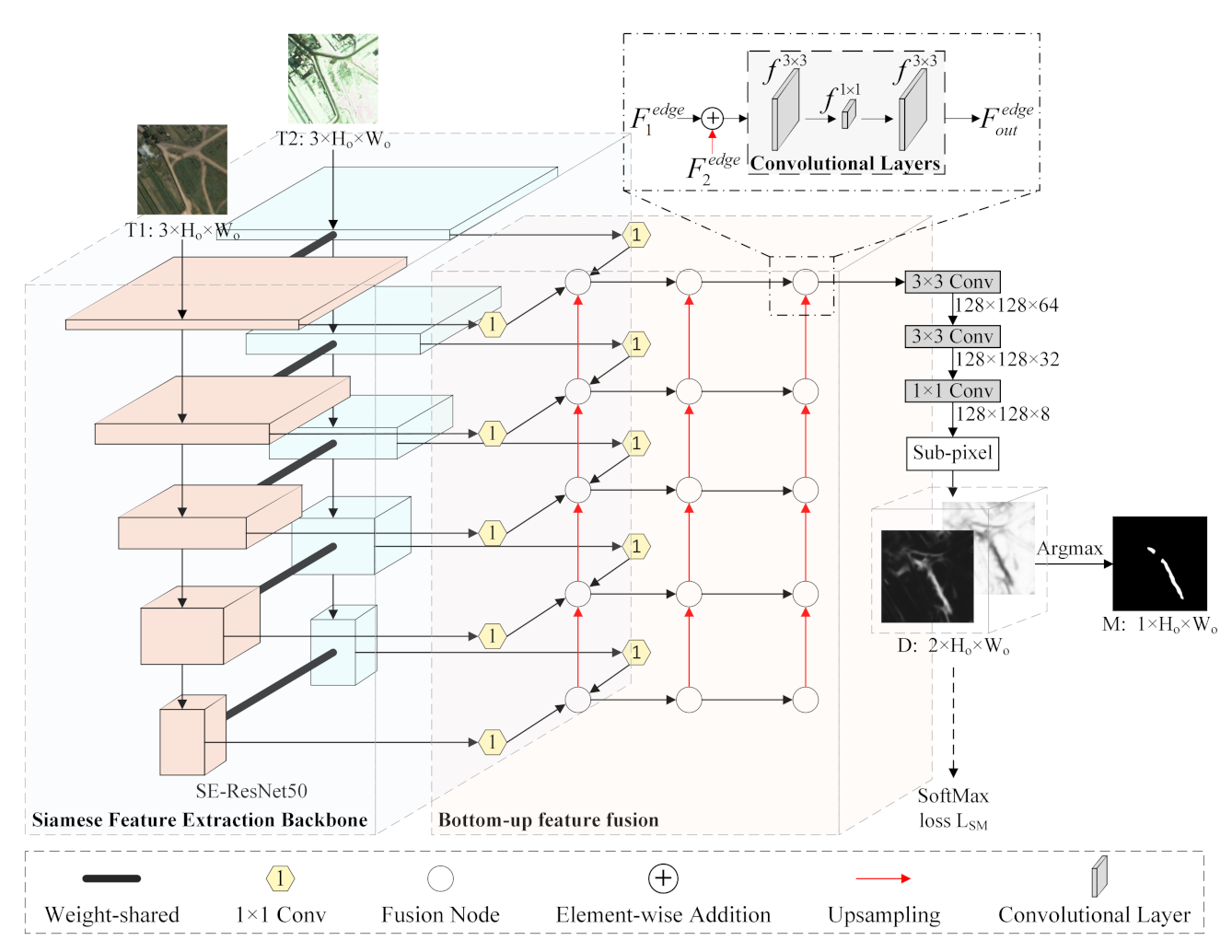
The overall architecture of the proposed MFPNet is shown in Figure 2.

First, bi-temporal image pairs (T1 and T2) are fed into a Siamese feature extraction backbone with two weight-shared SE-ResNet50s [43] to extract multi-level deep features. Then, features from those two backbones are sent into the proposed MAFFM for cross-level feature fusion. 1 × 1 convolutional layers in the MAFFM are used to unify the channel number of features from different levels, which is set as 256 in this paper. For every fusion node we conduct an AWF strategy, which aggregates different features (e.g., $F_1^{edge}$, $F_2^{edge}$, $F_3^{edge}$) from bottom-up, top-down, and shortcut-connection paths to generate weight refined fusion features $F_{out}^{edge}$. Afterwards, the final fusion features are upsampled by a sub-pixel method [67] back to the size of input images to generate the discriminative map $D\in {\mathbb{R}}^{2\times H_o\times W_o}$, where 2 is the number of classes (i.e., changed/unchanged), and $H_o$ and $W_o$, respectively, represent the original height and width of the input image. The main reason to adopt the sub-pixel method is that this upsampling technique is capable of self-learning contributing to a fine and complex mapping between low-resolution and high-resolution. The proposed PSM measures the perceptual similarity between the discriminative map D and its ground truth in feature spaces to shorten their distance. Finally, we apply an Argmax operation on D to pick the class of maximum score for each pixel to generate the change map M.

3.2. Multidirectional Adaptive Feature Fusion Module

To achieve cross-level feature aggregation sufficiently and efficiently, we propose a MAFFM including a multidirectional fusion pathway and an adaptive weighted fusion strategy.

3.2.1. Multidirectional Fusion Pathway

A conventional bottom-up multi-level fusion network is inherently limited by the one-way information flow [68]. To address this issue, we construct the multidirectional fusion pathway (MFP, shown in Figure 3), aiming at enriching the information flow of feature fusion. More specifically, we build an extra top-down fusion path (i.e., the blue line in Figure 3) to increase the flexibility and diversity of information paths. Extra shortcut connections (i.e., the green line in Figure 3) are added between fusion nodes in the first and third columns to shorten the information propagation and fuse more features. The feature fusion strategy becomes crucial to the MFP, which is composed of many fusion nodes. Simple multi-level fusion strategies, such as summation, subtraction, or concatenation operations, are widely used in existing RSCD networks. However, they ignore the semantic relationship between different features [44] and cannot exclude redundant information [12]. To overcome these issues, we introduce a novel feature fusion strategy named adaptive weighted fusion in the following section.

3.2.2. Adaptive Weighted Fusion

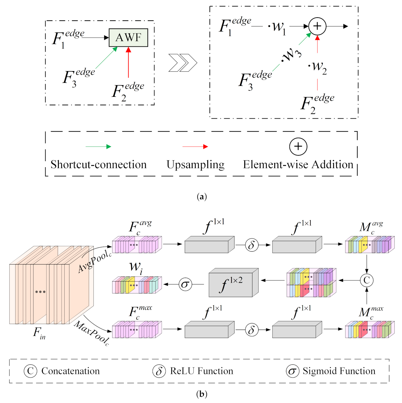
Fusion nodes in the MFP accept features from two or three edges. Since the input features of different edges come from different levels and periods, they usually contribute to the output feature unequally. We thus propose an adaptive weighted fusion (AWF) strategy for fusion nodes to fuse different features. The AWF strategy can be seen in Figure 4, which aims to recalibrate the weights of every input feature map adaptively before adding them together. Taking a fusion node that receives features from three edges as an example (shown in Figure 4a), it can be expressed as:

$$AWF\left(F_1^{edge},F_2^{edge},F_3^{edge}\right)=\left(w_1·\left(F_1^{edge}\right)\right)\oplus \left(w_3·\left(F_3^{edge}\right)\right)\oplus \left(w_2·\left(Up\left(F_2^{edge}\right)\right)\right)$$

(1)

where ⊕ represents element-wise addition and $Up$ means nearest interpolation upsampling. $F_1^{edge}\in {\mathbb{R}}^{C_1\times H_1\times W_1}$, $F_2^{edge}\in {\mathbb{R}}^{C_2\times H_2\times W_2}$, $F_3^{edge}\in {\mathbb{R}}^{C_3\times H_3\times W_3}$ represent three input features of the fusion node ($C,H,W$ mean channel, height, width). $w_1\in {\mathbb{R}}^{C_1},w_2\in {\mathbb{R}}^{C_2}$, $w_3\in {\mathbb{R}}^{C_3}$ are three weight vectors that represent the importance of every channel of three input features.

In order to provide appropriate and learnable weight vector $w_i$, we utilize a channel attention algorithm in each input edge of the fusion node to generate a channel-wise attention map and take it as the weight vector. The channel attention algorithm is inspired by a previous study [59]. Figure 4b shows the detailed process of obtaining a weight vector $w_i$. Given the input features $F_{in}$, we first perform global average pooling and global max pooling on $F_{in}$ along with the channel dimension to obtain two different spatial context descriptors $F_c^{avg}$ and $F_c^{max}$. Then, $F_c^{avg}$ and $F_c^{max}$ are separately sent into two 1×1 convolutional layers to generate average-pooled feature $M_c^{avg}$ and max-pooled feature $M_c^{max}$. Afterwards, we fuse $M_c^{avg}$ and $M_c^{max}$ together to generate $w_i$ by using a 1×2 convolutional layer. Formally, this process can be computed by:

$$M_c^{avg}=f^{1\times 1}\left(\delta \left(f^{1\times 1}\left({AvgPool}_c\left(F_{in}\right)\right)\right)\right)$$

(2)

$$M_c^{max}=f^{1\times 1}\left(\delta \left(f^{1\times 1}\left({MaxPool}_c\left(F_{in}\right)\right)\right)\right)$$

(3)

$$w_i=\sigma \left(f^{1\times 2}\left(M_c^{avg}c{M}_c^{max}\right)\right)$$

(4)

where $f^{1\times 1}$ and $f^{1\times 2}$ denote 1 × 1 and 1 × 2 convolution operations, respectively. $\sigma (·)$ and $\delta (·)$ represent Sigmoid and ReLU functions, respectively. c means a concatenation operation.

The AWF strategy provides adaptive weight recalibration for feature fusion, which allows the model to consider the semantic relationships between multi-level features and focus on helpful feature maps as well as ignoring irrelevant feature maps.

3.3. Perceptual Similarity Module

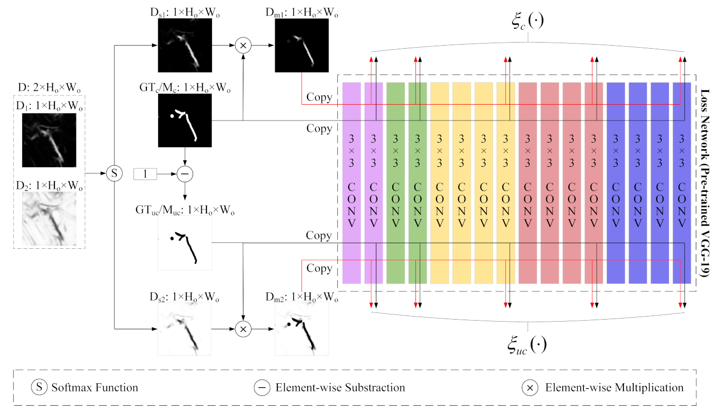
The predicted change map is determined by two feature maps $D_1$ and $D_2$ of the discriminative map D. By performing a SoftMax operation on D along the channel axis, $D_1$ and $D_2$ are transferred to $D_{s1}$ and $D_{s2}$, respectively. The value of each pixel of $D_{s1}$ represents the probability that the pixel belongs to the changed class, while that of $D_{s2}$ represents the probability that belongs to the unchanged class. Therefore, to obtain an accurate predicted change map, $D_{s1}$ should be consistent with the ground-truth changed regions label $G{T}_c$ while $D_{s2}$ should match with the ground-truth unchanged regions label $G{T}_{uc}$. Based on this fact, we propose a novel perceptual similarity module to calculate the perceptual loss of specific areas (i.e., the changed regions and the unchanged regions), which could embed perceptual information into our network and shorten the distance between $D_{s1}$ and $G{T}_c$, as well as the distance between $D_{s2}$ and $G{T}_{uc}$ in high-dimensional feature spaces. The detailed architecture of the PSM is shown in Figure 5. To compute the perceptual loss for a specific region, we need to generate binary masks that have a pixel value of 1 over the region of interest and 0 elsewhere. Since the ground-truth change map $GT$ has a pixel value of 1 in the changed area and 0 in the unchanged area, it can be used as the binary mask $M_c$ of changed regions and can also be regarded as the ground-truth changed regions label $G{T}_c$. The binary mask $M_{uc}$ of unchanged regions and the ground-truth unchanged regions label $G{T}_{uc}$ can be made by $1-GT$. Afterwards, $D_{s1}$ ($D_{s2}$) is element-wise multiplied by $M_c$ ($M_{uc}$), so that $D_{s1}$ ($D_{s2}$) is converted to a black and white masked feature map $D_{m1}$ ($D_{m2}$) where only the regions of interest are visible. Now, all non-zero distances in the feature space between the masked feature map $D_{m1}$ ($D_{m2}$) and its ground-truth $G{T}_c$ ($G{T}_{uc}$) correspond to the visible areas, i.e., the changed (unchanged) areas. Following the guidance of previous works [27,64], we utilize a VGG-19 model pre-trained on ImageNet as our fixed loss network to compute the perceptual loss. Low-level features of VGG-19 contain local information such as edges and textures, while high-level features of VGG-19 contain abstract information such as semantic concept and image content. Therefore, in order to obtain comprehensive information from the VGG-19 fixed loss network, we calculate distances in both low-level and high-level feature spaces of VGG-19 to form our perceptual loss. The function $\xi (·)$ to calculate the distances is defined as:

$$\xi \left(I_1,I_2\right)=\sum _{i,j}\frac{1}{C^{i,j}{H}^{i,j}{W}^{i,j}}{∥{\varphi }^{i,j}\left(I_1\right)-{\varphi }^{i,j}\left(I_2\right)∥}_2^2$$

(5)

where $I_1$, $I_2$ are two inputs, ${\varphi }^{i,j}$ is the output feature of the i-th group j-th ReLU layer of the VGG-19 loss network when processing the input x, and here we set $(i,j)$ as $\left\{\right(1,2),(2,2),(3,4)$, $(4,4),(5,4)\}$. C, H, W are the Channel, Height, Width of the corresponding output feature, respectively. ${\parallel ·\parallel }_2^2$ calculates the squared Euclidean distance point by point.

In summation, the process of the PSM can be formally expressed as:

$$PSM(D_1,D_2,GT)\left\{\begin{array}{c}\left(D_{s1},D_{s2}\right)=S\left(D_1,D_2\right)\hfill \\ M_c=G{T}_c=GT\hfill \\ M_{uc}=G{T}_{uc}=1-GT\hfill \\ \begin{array}{cc}\hfill L_P=& {\xi }_c\left(Copy\left(D_{s1}\otimes M_c,G{T}_c\right)\right)\hfill \\ \hfill & +{\xi }_{uc}\left(Copy\left(D_{s2}\otimes M_{uc},G{T}_{uc}\right)\right)\hfill \end{array}\hfill \end{array}\right.$$

(6)

where $D_{s1}$ and $D_{s2}$ are obtained by applying the SoftMax operation $S(·)$ over two feature maps $D_1$ and $D_2$ to each spatial location. ⊗ denotes element-wise multiplication. ${\xi }_c(·)$ and ${\xi }_{uc}(·)$ are the functions to calculate feature space distances between any two given inputs for changed regions and unchanged regions, respectively, which are defined in (5). $Copy$ means replicating input three times along the channel dimension to fit the input-shaped demand of the loss network. $L_P$ is the proposed perceptual loss, which is the sum of the squared Euclidean distance between ten feature representation pairs.

4. Experiments

In this section, we evaluate the proposed network MFPNet on four publicly available benchmark datasets to demonstrate its effectiveness. First, we introduce details of the four datasets, i.e., the Season-Varying dataset [69], the LEVIR-CD dataset [53], the Google dataset [12], and the Zhang dataset [58]. Second, we present implementation details including loss function and evaluation metrics. Third, eight state-of-the-art comparative methods are introduced. Afterwards, we quantitatively and qualitatively compare our results against those eight methods for four datasets. Finally, discussions are conducted to show the effectiveness of the proposed modules.

4.1. Remote Sensing Change Detection Datasets

The Season-Varying dataset [69] has 7 pairs of VHR season-varying images with 4725 × 2200 pixels for manual ground truth creation, and 4 pairs of images with 1900 × 1000 pixels for adding additional objects manually. This dataset considers objects of different sizes (such as roads, buildings, and vehicles) while ignoring the changes caused by seasonal differences, brightness, and other factors. The spatial resolution of images varies from 3 to 100 cm/pixel, and the weather and seasonal differences between bi-temporal images vary largely. The dataset has been clipped into 256 × 256 nonoverlapping image patches by its original author to generate 16,000 sub-image pairs of which 10,000 are for training, 3000 are for validation, and 3000 are for testing.

The LEVIR-CD dataset [53] consists of 637 VHR (50 cm/pixel) image pairs with a size of 1024 × 1024 pixels. These bi-temporal images with a time span of 5 to 14 years cover the changes of various buildings, such as garages, warehouses, and villas. Additionally, these images are from 20 different regions that sit in several cities in Texas in the US, including Austin, Lakeway, Bee Cave, Buda, Kyle, Manor, Pflugervilletx, Dripping Springs, etc. The dataset has been divided into training, validation, and test sets by its author. Following the illustration in the original literature [53], we cropped each sample to 16 small patches of size of 256 × 256 to generate 7120 image patch pairs for training, 1024 for validation, and 2048 for testing.

The third dataset, named the Google dataset [12], consists of 20 season-varying VHR image pairs with a spatial resolution of 55 cm, and sizes ranging from 1006 × 1168 pixels to 5184 × 6736 pixels. This dataset covers the suburb areas of Guangzhou City, China, and is used for building change detection. It is divided into 256 × 256 pixel nonoverlapping patches with at least a fraction of changed pixels, where 1156 pairs of sub-images are generated. The sub-image pairs were randomly divided according to a ratio of 7:2:1 to generate training, validation, and test sets. Afterwards, the training set was rotated by 90${}^{\circ }$, 180${}^{\circ }$, and 270${}^{\circ }$, and flipped in horizontal and vertical directions for data augmentation. Finally, we obtained 4848 sub-image pairs for training, 232 for validation, and 116 for testing.

The fourth dataset [58] consists of 6 large co-registered bi-temporal image pairs collected from six different cities in China, denoted as the Zhang dataset. These season-varying images provided by Google Earth were collected by a variety of sensors, resulting in a dataset with varied image brightness and contrast. It focuses on the appearance and disappearance of landcover objects, such as water bodies, roads, croplands, and buildings, while ignoring the changes caused by seasons changing, image brightness, and other factors. As illustrated in the relevant paper [58], this dataset, generated by cropping and augmenting, contains 3600 bi-temporal sub-image pairs in the training set, 340 pairs in the validation set, 48 pairs in the test set. The size of each sub-image is 512 × 512 pixels, and the resolution is 200 cm/pixel. It is worth noting that the training set and validation set of this dataset are from Beijing, Chengdu, Shenzhen, Chongqing, and Wuhan, while the test set is entirely from another city (i.e., Xi’an), aiming to test the generalization ability of change detection models.

4.2. Implementation Details

We implemented our proposed method with PyTorch, supported by an NVIDIA CUDA with a GeForce GTX 1080Ti GPU. In the training phase, the Siamese feature extraction backbone and the PSM of the proposed MFPNet were respectively initialized from the SE-ResNet50 [43] and the VGG-19 [26], which were both pre-trained on the ImageNet dataset [70]. We adopted the Adam optimizer and set the base learning rate to 1 × 10⁻⁴. The learning rate was decayed with a cosine annealing schedule [71]. The batch size was set to 4, except for the Zhang dataset where the batch size was set to 2 for the benefit of GPU training. Model training finished when the F1-score for the validation set did not improve for 40 epochs.

4.2.1. Loss Function

In the training phase, we applied SoftMax PPCE loss $L_{SM}$ and the proposed perceptual loss $L_P$ as our loss function. SoftMax PPCE loss is one of the most commonly used loss functions for RSCD. Let us consider a training sample $\left\{\left(X^{T1},X^{T2}\right),Y\right\}$, where $\left(X^{T1},X^{T2}\right)$ are the bi-temporal images, and Y is the ground-truth change map. $L_{SM}$ can be defined as $L_{SM}=-\frac{1}{J}{\sum }_{j=0}^J{\sum }_{c=0}^{1}logPr\left(Y_j=c\mid \left(X^{T1},X^{T2}\right);\theta \right)$, where the sums run over the total J pixels; $Pr\left(Y_j=c\mid \left(X^{T1},X^{T2}\right);\theta \right)$ presents the predicted probability of pixel j belonging to the c-th class, which is obtained by the SoftMax function. Since there are only two classes in our task, c is set to 1 or 0 to indicate the changed class or the unchanged class. Our perceptual loss is computed by the proposed PSM and its detailed definition can be seen in (6). In summary, the total loss function for our proposed framework MFPNet is $L=L_{SM}+\lambda L_P$, where $\lambda$ denotes the weight of perceptual loss and is set as 1 × 10⁻⁴ in this paper.

4.2.2. Evaluation Metrics

For quantitative assessment, two indices, namely F1-score (F1) and Kappa coefficient (Kappa) are used as the evaluation metrics. These two indices can be calculated as follows:

$$\mathrm{F}1=\frac{2\times \mathrm{Precision}\times \mathrm{Recall}}{\mathrm{Precision}+\mathrm{Recall}},\mathrm{Precision}=\frac{\mathrm{TP}}{\mathrm{TP}+\mathrm{FP}},\mathrm{Recall}=\frac{\mathrm{TP}}{\mathrm{TP}+\mathrm{FN}}$$

(7)

$$\mathrm{Kappa}=\frac{\mathrm{OA}-\mathrm{PRE}}{1-\mathrm{PRE}}$$

(8)

$$\mathrm{OA}=\frac{\mathrm{TP}+\mathrm{TN}}{\mathrm{TP}+\mathrm{FP}+\mathrm{TN}+\mathrm{FN}}$$

(9)

$$\mathrm{PRE}=\frac{(\mathrm{TP}+\mathrm{FN})\times (\mathrm{TP}+\mathrm{FP})+(\mathrm{TN}+\mathrm{FP})\times (\mathrm{TN}+\mathrm{FN})}{{(\mathrm{TP}+\mathrm{FP}+\mathrm{TN}+\mathrm{FN})}^2}$$

(10)

where OA and PRE denote the overall accuracy and expected accuracy, respectively. TP, FP, TN, and FN are the number of true positives, false positives, true negatives, and false negatives, respectively. It is noteworthy that F1 is a weighted harmonic mean of precision and recall, which balances the conflict by considering precision and recall simultaneously and can better reflect the change detection ability of a model [33]. Higher F1-score and Kappa represent better overall performance of the model [12].

4.3. Comparative Methods

Eight current networks specially designed for RSCD were selected as the comparative methods. Their key characteristics are summarized in

Table 1. Key characteristics of comparative methods.

Networks	Published Year	Architecture	Loss Function	Feature Fusion Strategy
FC-Siam-conc [45]	2018	Siamese, FCN	Weighted SoftMax PPCE loss	Multi-level fusion, concatenation, skip-connection
FC-Siam-diff [45]	2018	Siamese, FCN	Weighted SoftMax PPCE loss	Multi-level fusion, subtraction, skip-connection
FCN-PP [37]	2019	Single-branch, FCN	SoftMax PPCE loss	Early-fusion, concatenation, skip-connection
UNet++_MSOF [34]	2019	Single-branch, UNet++	Weighted sigmoid PPCE loss, dice loss	Early-fusion, concatenation, dense skip-connection
STANet [53]	2020	Siamese, ResNet	Batch-balanced contrastive loss	Mid-fusion, self-attention
DSIFN [58]	2020	Siamese, VGG	Sigmoid PPCE loss, dice loss	Multi-level fusion, channel and spatial attention
SNUNet-CD/48 [13]	2021	Siamese, UNet++	Weighted SoftMax PPCE loss, dice loss	Multi-level fusion, channel attention, dense skip-connection
LSS-Net [66]	2021	Siamese, SE-ResNet	SoftMax PPCE loss, perceptual loss	Multi-level fusion, local similarity attention

. Note that UNet++_MSOF [34] and DSIFN [58] use deep supervision in their intermediate layers as a training trick to accelerate the training process and enhance network performance. Because Fang et al. [13] proposed six SNUNet-CD networks with different widths, here we take the “SNUNet-CD/48” network, which has the best performance among the six SNUNet-CD networks, as our comparative method.

4.4. Evaluation for the Season-Varying Dataset

The quantitative results for the Season-Varying dataset are shown in

Table 2. Quantitative results for the Season-Varying dataset. The best two results are in bold and underline.

Methods	Season-Varying Dataset
	F1 (%)	Kappa (%)
FC-Siam-conc [45]	68.25	65.27
FC-Siam-diff [45]	70.06	69.12
FCN-PP [37]	84.95	83.04
UNet++_MSOF [34]	89.93	88.63
STANet [53]	91.31	90.10
DSIFN [58]	90.65	89.45
SNUNet-CD/48 [13]	96.20	95.70
LSS-Net [66]	96.30	95.81
MFPNet (ours)	97.54	97.21

. It can be seen that MFPNet achieves the best performance with the highest F1 (97.54%) and Kappa (97.21%). Compared with other methods, MFPNet exhibits significant improvements by at least 1.24% and 1.4% in terms of F1 and Kappa, respectively.

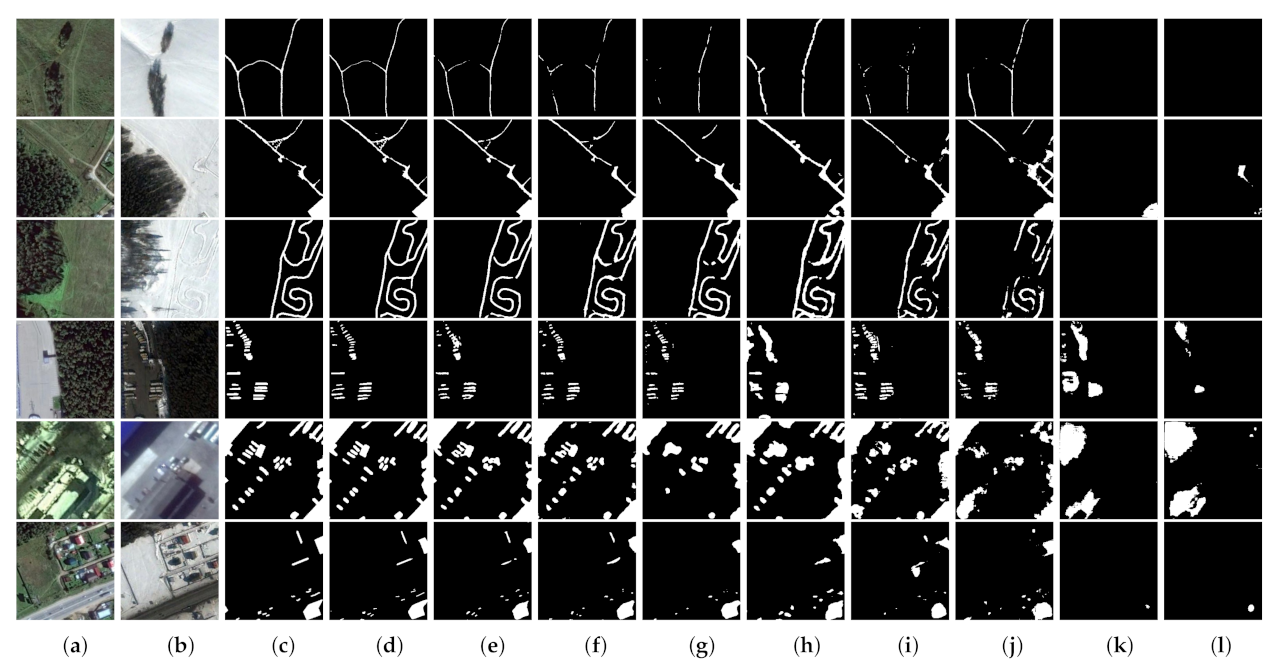
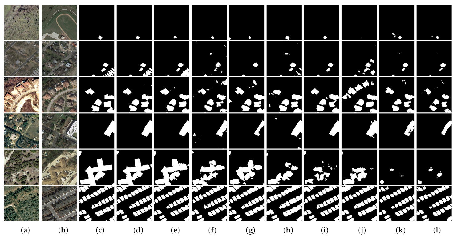
The Season-Varying dataset has changeable scenes and different change objects. Figure 6 and Figure 7 show several representative results for qualitative analysis. As one can see, although there is significant noise between bi-temporal images T1 and T2 (such as the disturbance of solar altitude, snow, and sensors), MFPNet successfully filters such irrelevant factors and identifies real changed areas. Regarding the thin and small areas, such as narrow roads, vehicles, and small buildings, MFPNet can distinguish more tiny changes, leading to high-quality change maps with good continuity and clear boundaries, as seen in Figure 6. For large and complex area changes, MFPNet outperforms other methods in object integrity maintenance and detail restoration, as seen in Figure 7. In summary, the proposed MFPNet achieves the best visual performance on the Season-Varying dataset and its change maps are more consistent with the ground truth.

4.5. Evaluation for the LEVIR-CD Dataset

Table 3. Quantitative results for the LEVIR-CD dataset. The best two results are in bold and underline.

Methods	LEVIR-CD Dataset
	F1 (%)	Kappa (%)
FC-Siam-conc [45]	81.44	80.58
FC-Siam-diff [45]	83.78	82.99
FCN-PP [37]	89.10	88.51
UNet++_MSOF [34]	88.94	88.36
STANet [53]	88.07	87.41
DSIFN [58]	90.12	89.60
SNUNet-CD/48 [13]	88.80	88.21
LSS-Net [66]	90.43	89.93
MFPNet (ours)	91.69	91.25

presents the quantitative results for different methods for the LEVIR-CD dataset. We can conclude that the proposed MFPNet achieves the best performance against other comparative methods, exhibiting the highest scores on both metrics. Specifically, the F1 and Kappa values of the MFPNet are 91.69% and 91.25%, respectively. Compared with the second-best model, DSIFN, the MFPNet yields improvements of 1.26% and 1.32% for F1 and Kappa, respectively.

Note that only building changes are labeled in this dataset and the results obtained on typical test samples are shown in Figure 8. It can be seen that our MFPNet is good at capturing scattered as well as dense building changes. In particular, MFPNet can focus on building changes and sufficiently overcome the interference of other changes such as roads and trees, thus outputting finer details with less noise, e.g., rows 1–3 of Figure 8. In addition, MFPNet learns the characteristics of buildings accurately, and thus maintains the integrity and geometric edges of buildings in the change maps, e.g., rows 4–6 of Figure 8.

4.6. Evaluation for the Google Dataset

Table 4. Quantitative results for the Google dataset. The best two results are in bold and underline.

Methods	Google Dataset
	F1 (%)	Kappa (%)
FC-Siam-conc [45]	80.08	74.31
FC-Siam-diff [45]	78.43	71.62
FCN-PP [37]	82.69	77.27
UNet++_MSOF [34]	80.44	74.29
STANet [53]	74.72	68.38
DSIFN [58]	84.54	79.85
SNUNet-CD/48 [13]	76.26	67.90
LSS-NET [66]	85.76	81.22
MFPNet (ours)	87.09	83.01

shows the performance of different methods for the Google dataset. The comparison results show that MFPNet outperforms the other eight methods by 1.33–12.37% in F1 and 1.79–15.11% in Kappa, yielding a result of 87.09% in F1 and 83.01% in Kappa.

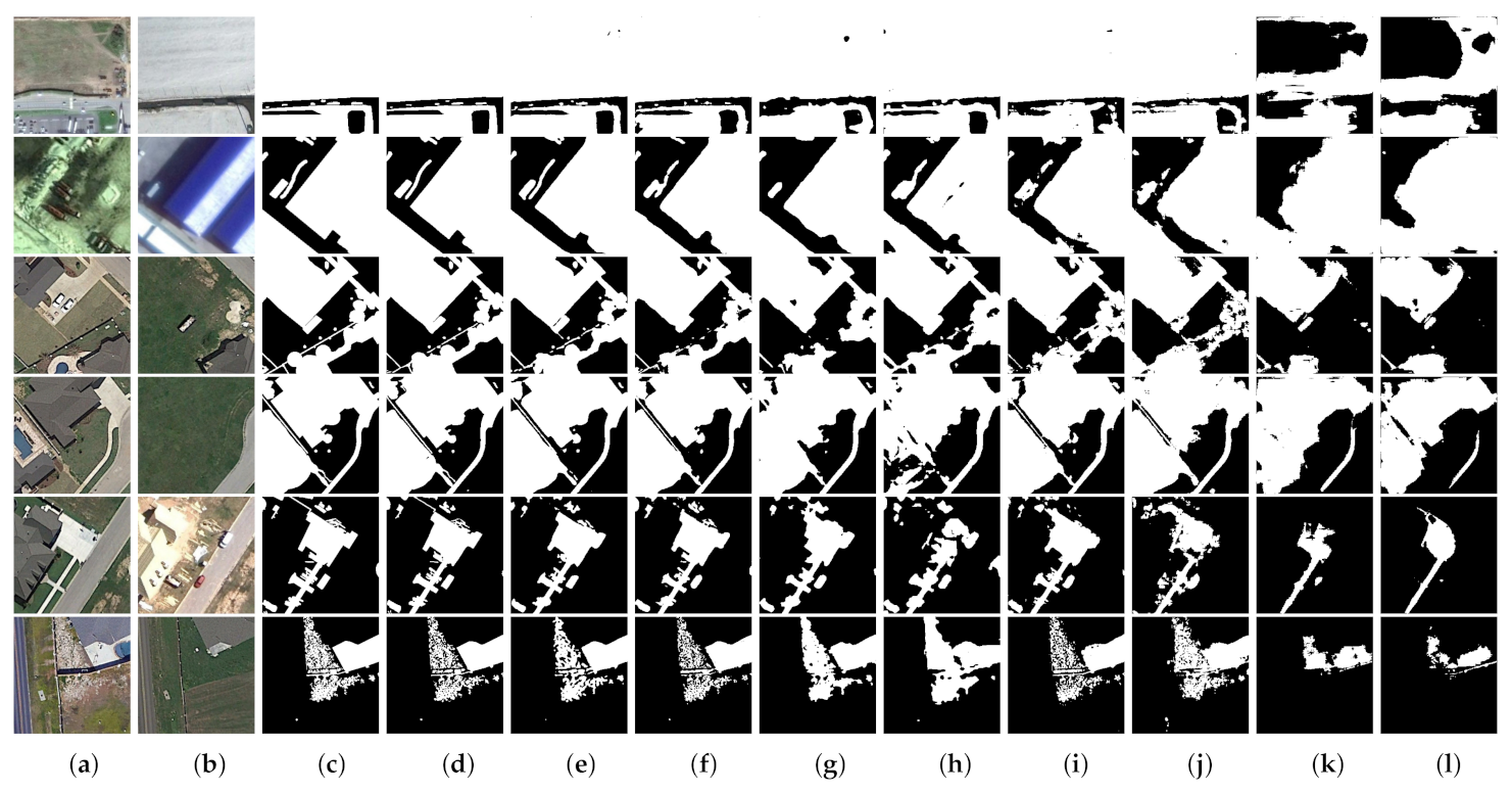
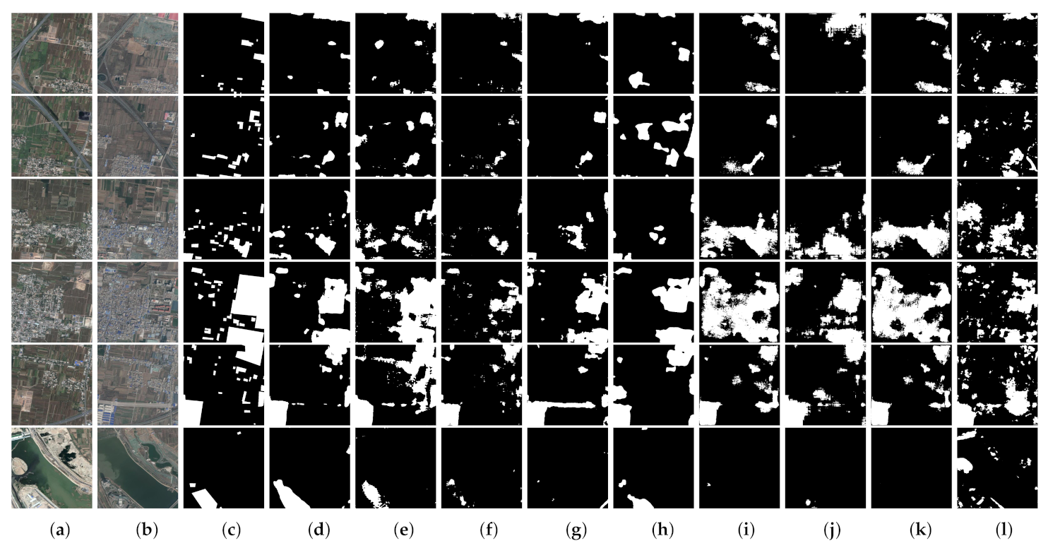
For the purpose of qualitative comparison of different methods for the Google dataset, some typical results are illustrated in Figure 9. It can be seen that all the methods can detect the changed buildings with different sizes. The proposed MFPNet achieves the best visual performance among all the algorithms by reducing false and missed detections, resulting in finer change maps with more accuracy and less noise. In particular, while the other algorithms exhibit false detections like mistaking road changes, shadow changes, or vehicle changes as building changes, MFPNet can better remove those false alarms to produce more precision change maps, as presented in the first three rows of Figure 9. Further, missed detections of building changes can be better overcome by MFPNet, as presented in the last three rows of Figure 9.

4.7. Evaluation for the Zhang Dataset

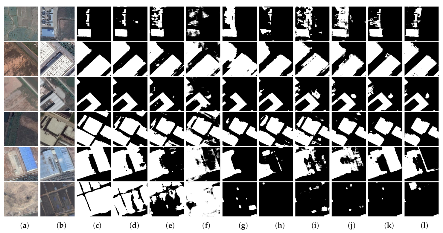
To further verify the generalization ability of the proposed MFPNet, we conducted experiments on the Zhang dataset. Note that the samples used in the test set are from a different city that is not used in the training or validation sets. The huge inconsistency of data distribution between training/validation sets and the test set raises a big challenge for RSCD algorithms. Nevertheless, our proposed MFPNet still obtains the highest F1 (68.45%) and Kappa (62.01%) with 0.69–18.37% and 0.53–24.12% improvements, respectively, as shown in

Table 5. Quantitative results for the Zhang dataset. The best two results are in bold and underline.

Methods	Zhang Dataset
	F1 (%)	Kappa (%)
FC-Siam-conc [45]	50.08	37.89
FC-Siam-diff [45]	59.27	51.58
FCN-PP [37]	61.23	52.75
UNet++_MSOF [34]	62.69	54.52
STANet [53]	63.43	55.78
DSIFN [58]	67.76	61.01
SNUNet-CD/48 [13]	67.48	61.48
LSS-Net [66]	63.14	53.80
MFPNet (ours)	68.45	62.01

.

The visualization is shown in Figure 10. Due to the great challenge brought by this dataset, all the algorithms perform poorly for small object change detection, but our proposed MFPNet still outperforms the best methods by a small margin. For large area change detection, the change maps of the MFPNet contain higher object compactness and clearer boundaries.

5. Discussion

The experimental results above show the potential of the proposed network MFPNet in RSCD. In this section, we further discuss the rationality of the proposed approaches, the limitations of the proposed network, and the plan for our future work.

5.1. Rationality of the Proposed Approaches

To demonstrate the benefits of our proposed approaches, we conducted an ablation study by adding each proposed component individually to the baseline as well as incorporating all the components progressively, including the MFP, AWF, and PSM. The detailed architecture of the baseline is presented in Figure 11, consisting of the Siamese SE-ResNet50 feature extraction backbone and three bottom-up feature fusion pathways. For every fusion node, three convolutional layers perform 3 × 3, 1 × 1, and 3 × 3 convolutional operations. The results are listed in

Table 6. Ablation results for the proposed MFPNet for four dataset. The best two results are in bold and underline.

Framework	MFP	AWF	PSM	Season-Varying Dataset		LEVIR-CD Dataset		Google Dataset		Zhang Dataset
				F1 (%)	Kappa (%)	F1 (%)	Kappa (%)	F1 (%)	Kappa (%)	F1 (%)	Kappa (%)
Baseline				96.16	95.65	87.15	86.45	78.02	71.90	60.87	53.79
Baseline_MFP				96.79	96.36	89.04	88.47	83.65	78.82	64.29	57.34
Baseline_AWF				97.01	96.60	88.82	88.25	82.28	77.02	65.40	56.81
Baseline_PSM				96.90	96.48	90.90	90.42	81.84	76.36	63.98	56.54
Baseline_MAFFM				97.29	96.92	90.32	89.81	84.79	79.66	66.90	58.97
MFPNet (ours)				97.54	97.21	91.69	91.25	87.09	83.01	68.45	62.01

. We also applied the proposed AWF and PSM to other existing RSCD networks to explore their versatility and portability. Specific analysis is as follows.

5.1.1. Effect of the MFP

To verify the MFP, we added it to the baseline by changing the second path of the bottom-up feature fusion from bottom-up to top-down and augmenting extra short-connection paths. It is noteworthy that the above-mentioned operation only changes the fusion pathway without introducing any additional convolutional layer. As shown in Table 6, the MFP brings 0.63%, 1.89%, 5.63%, and 3.42% F1 improvements for the baseline on the Season-Varying, LEVIR-CD, Google, and Zhang datasets, respectively. In addition, the MFP gains 0.71%, 2.02%, 6.92%, and 3.55% in Kappa. These results confirm that the conventional bottom-up multi-level fusion network is inherently limited by the one-way information flow and prove the effectiveness of fusing features from multi-directional pathways.

5.1.2. Effect of the AWF

The proposed AWF provides additional weights, which reflect the importance of features, for each input before fusing them together. To evaluate the benefit of the AWF, we applied the AWF strategy to each fusion node of the baseline and the baseline_MFP to form the baseline_AWF and baseline_MAFFM, respectively. As shown in Table 6, the AWF strategy gains 0.85%, 1.67%, 4.26%, and 4.53% in F1 and 0.95%, 1.8%, 5.12%, and 3.02% in Kappa compared with the baselines of the four datasets. The baseline_MAFFM using both MFP and AWF achieves better performance than the networks using only MFP or AWF, which shows that the advantages of the proposed MFP and AWF approaches are complementary and their coherent innovations contribute to a high-performance RSCD model. Furthermore, the idea of AWF can be used directly in existing CNN-based techniques to conduct weight recalibration. To explore the versatility and portability of the AWF strategy, we applied it to FC-Siam-conc [45] and FC-Siam-diff [45] on the Season-Varying dataset. As reported in

Table 7. Performance comparison of FC-Siam-conc and FC-Siam-diff with/without AWF on Season-Varying dataset. The number in the brackets means the gain brought by adding the AWF strategy.

Methods	F1 (%)	Kappa (%)
FC-Siam-conc [45] (+AWF)	68.25 (+5.94)	65.27 (+5.98)
FC-Siam-diff [45] (+AWF)	70.06 (+3.73)	69.12 (+1.96)

, the models with AWF consistently outperformed the models without AWF, which confirms the usefulness of the AWF strategy on other RSCD networks. The above facts indicate that simple feature fusion manners like addition (provided by Baseline and Baseline_MFP), concatenation (provided by FC-Siam-conc), and subtraction (provided by FC-Siam-diff) are not effective for the RSCD task. It is more sensible to fuse different features after weighted calibration, which can be achieved by our AWF strategy.

5.1.3. Effect of the PSM

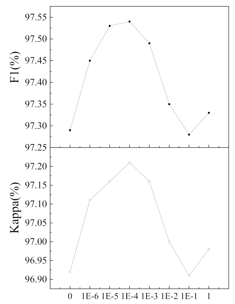
The proposed PSM introduces perceptual loss for changed regions and unchanged regions to encourage predicted change maps to be perceptually similar to ground-truth images. As shown in Table 6, the PSM boosts 0.74%, 3.75%, 3.82%, and 3.11% in F1 and 0.83%, 3.97%, 4.46%, and 2.75% in Kappa compared with the baseline. The introduction of PSM to the baseline_MAFFM also enhances its performance. The above facts demonstrate the effectiveness of the PSM. To explore the sensitivity of the proposed perceptual loss gained by the PSM, we adapted the hyperparameter $\lambda$ of the proposed perceptual loss from 1 × 10⁻⁶ to 1 for the Season-Varying dataset. As shown in Figure 12, when $\lambda$ is set to 0, only SoftMax PPCE loss is used for model training, resulting in low F1 and Kappa. With the increasing number of $\lambda$, the values of F1 and Kappa increase gradually, showing the great potential of perceptual loss in the RSCD task. The performance reaches the peak when $\lambda$ approaches 1 × 10⁻⁴, and then it decreases in a fluctuating way, implying that too much perceptual loss can impair prediction results. To explore the versatility and portability of the PSM, we applied it to FC-Siam-conc and FC-Siam-diff.

Table 8. Performance comparison of FC-Siam-conc and FC-Siam-diff with/without PSM. The number in the brackets mean the gain brought by the addition of PSM.

Methods	F1 (%)	Kappa (%)
FC-Siam-conc [45] (+PSM)	68.25 (+3.34)	65.27 (+3.63)
FC-Siam-diff [45] (+PSM)	70.06 (+3.86)	69.12 (+1.98)

shows the quantitative performance. We can see that PSM boosts the F1 of FC-Siam-conc and FC-Siam-diff by 3.34% and 3.86%, respectively. The PSM increases their Kappa values as well. This fact further confirms that PSM is beneficial for the RSCD task.

Viewing Table 6 as a whole, the best performance is delivered by our proposed framework, MFPNet. Specifically, with all these components in MFPNet, improvements on F1 are 1.38%, 4.54%, 9.07%, and 7.58%, and on Kappa are 1.56%, 4.80%, 11.11%, and 8.22% over the baseline on the Season-Varying, LEVIR-CD, Google, and Zhang datasets, respectively. It is noteworthy that although our proposed network, MFPNet, is verified on RGB images, the MFPNet itself is independent of raster data types, which means our network can be extended to other forms of two-dimensional raster data (such as near-infrared, spectral, or hyperspectral images) for RSCD.

5.2. Limitations of the Proposed Network

Although the proposed network, MFPNet, achieves promising performance, it has some potential limitations. First, the computational complexity of the MFPNet is relatively high, which is unfriendly to resource-constrained equipment and applications. As shown in

Table 9. Model complexity. M: million. B: billion. MAdds: multiple-adds measured with regard to a 256 × 256 input.

Method	Parameters (M)	MAdds (B)
FC-Siam-conc [45]	1.55	5.32
FC-Siam-diff [45]	1.35	4.72
FCN-PP [37]	18.70	36.52
UNet++_MSOF [34]	9.06	26.03
STANet [53]	16.93	13.17
DSIFN [58]	35.73	82.35
SNUNet-CD/48 [13]	27.07	123.21
LSS-NET [66]	45.66	59.13
MFPNet (ours)	60.05	107.48

, the number of trainable parameters of the MFPNet is 60.05 million, which is the largest one among comparative methods. As for the number of multiply–add operations (MAdds), MFPNet is smaller than SNUNet-CD and larger than the other models. Thus, some model compression techniques, such as pruning and knowledge distillation, could be exploited for our network to reduce the model size. Second, the proposed network is designed for monomodal change detection, which could be further developed for multimodal change detection.

5.3. Future Work

As discussed in Section 5.2, we intend to exploit the potential of model compression techniques to reduce the model complexity. In addition, we will explore the availability of multimodal data fusion and adversarial training in RSCD, so as to further improve the performance and robustness of change detection models to various types of noise (e.g., clouds and smoke occlusions).

6. Conclusions

In this paper, we proposed a novel deep learning network (MFPNet) for RSCD. To enhance the process of feature fusion, we proposed an MAFFM that consists of an MFP and an AWF strategy. The MFP improves the diversity of information paths and eases information propagation. The AWF strategy emphasizes important feature maps as well as suppressing irrelevant feature maps for reliable information passing; thus, the comprehensive and high-quality features can be aggregated at each fusion node. Furthermore, to compensate for the drawbacks of PPCE loss, we proposed a PSM to calculate the perceptual loss for changed and unchanged areas. The PSM provides perceptual information for the network and minimizes the distance between the predicted change map and its ground truth in high-dimensional feature spaces, thus making the output consistent with its ground truth. The effectiveness and robustness of the proposed network were verified for four benchmark datasets that have different change targets as well as imaging conditions. Experimental results show that the proposed network (MFPNet) achieves the best performance in both quantitative assessment and visual interpretation among state-of-the-art methods.

References

- Fang, B.; Chen, G.; Pan, L.; Kou, R.; Wang, L. GAN-Based Siamese Framework for Landslide Inventory Mapping Using Bi-Temporal Optical Remote Sensing Images. IEEE Geosci. Remote Sens. Lett. 2021, 18, 391–395. [Google Scholar] [CrossRef]
- Sublime, J.; Kalinicheva, E. Automatic post-disaster damage mapping using deep-learning techniques for change detection: Case study of the Tohoku tsunami. Remote Sens. 2019, 11, 1123. [Google Scholar] [CrossRef] [Green Version]
- Saha, S.; Bovolo, F.; Bruzzone, L. Building Change Detection in VHR SAR Images via Unsupervised Deep Transcoding. IEEE Trans. Geosci. Remote Sens. 2021, 59, 1917–1929. [Google Scholar] [CrossRef]
- Papadomanolaki, M.; Vakalopoulou, M.; Karantzalos, K. A Deep Multitask Learning Framework Coupling Semantic Segmentation and Fully Convolutional LSTM Networks for Urban Change Detection. Available online: https://0-ieeexplore-ieee-org.brum.beds.ac.uk/document/9352207 (accessed on 10 February 2021).
- Khan, S.H.; He, X.; Porikli, F.; Bennamoun, M. Forest Change Detection in Incomplete Satellite Images with Deep Neural Networks. IEEE Trans. Geosci. Remote Sens. 2017, 55, 5407–5423. [Google Scholar] [CrossRef]
- Isaienkov, K.; Yushchuk, M.; Khramtsov, V.; Seliverstov, O. Deep Learning for Regular Change Detection in Ukrainian Forest Ecosystem With Sentinel-2. IEEE J. Sel. Top. Appl. Earth Observ. Remote Sens. 2021, 14, 364–376. [Google Scholar] [CrossRef]
- Awty-Carroll, K.; Bunting, P.; Hardy, A.; Bell, G. An Evaluation and Comparison of Four Dense Time Series Change Detection Methods Using Simulated Data. Remote Sens. 2019, 11, 2779. [Google Scholar] [CrossRef] [Green Version]
- Han, Y.; Javed, A.; Jung, S.; Liu, S. Object-Based Change Detection of Very High Resolution Images by Fusing Pixel-Based Change Detection Results Using Weighted Dempster–Shafer Theory. Remote Sens. 2020, 12, 983. [Google Scholar] [CrossRef] [Green Version]
- Ghaderpour, E.; Vujadinovic, T. Change Detection within Remotely Sensed Satellite Image Time Series via Spectral Analysis. Remote Sens. 2020, 12, 4001. [Google Scholar] [CrossRef]
- Bruzzone, L.; Bovolo, F. A Novel Framework for the Design of Change-Detection Systems for Very-High-Resolution Remote Sensing Images. Proc. IEEE 2013, 101, 609–630. [Google Scholar] [CrossRef]
- Chen, H.; Wu, C.; Du, B.; Zhang, L.; Wang, L. Change Detection in Multisource VHR Images via Deep Siamese Convolutional Multiple-Layers Recurrent Neural Network. IEEE Trans. Geosci. Remote Sens. 2020, 58, 2848–2864. [Google Scholar] [CrossRef]
- Peng, D.; Bruzzone, L.; Zhang, Y.; Guan, H.; Ding, H.; Huang, X. SemiCDNet: A Semisupervised Convolutional Neural Network for Change Detection in High Resolution Remote-Sensing Images. IEEE Trans. Geosci. Remote Sens. 2020, 59, 5891–5906. [Google Scholar] [CrossRef]
- Fang, S.; Li, K.; Shao, J.; Li, Z. SNUNet-CD: A Densely Connected Siamese Network for Change Detection of VHR Images. Available online: https://paperswithcode.com/paper/snunet-cd-a-densely-connected-siamese-network (accessed on 17 February 2021).
- Singh, A. Change detection in the tropical forest environment of northeastern India using Landsat. Remote Sens. Trop. Land Manag. 1986, 44, 273–254. [Google Scholar]
- Todd, W.J. Urban and regional land use change detected by using Landsat data. J. Res. US Geol. Surv. 1977, 5, 529–534. [Google Scholar]
- Ridd, M.K.; Liu, J. A Comparison of Four Algorithms for Change Detection in an Urban Environment. Remote Sens. Environ. 1998, 63, 95–100. [Google Scholar] [CrossRef]
- Bovolo, F.; Bruzzone, L. A Theoretical Framework for Unsupervised Change Detection Based on Change Vector Analysis in the Polar Domain. IEEE Trans. Geosci. Remote Sens. 2007, 45, 218–236. [Google Scholar] [CrossRef] [Green Version]
- Celik, T. Unsupervised Change Detection in Satellite Images Using Principal Component Analysis and k-Means Clustering. IEEE Geosci. Remote Sens. Lett. 2009, 6, 772–776. [Google Scholar] [CrossRef]
- Nielsen, A.A. The Regularized Iteratively Reweighted MAD Method for Change Detection in Multi- and Hyperspectral Data. IEEE Trans. Image Process. 2007, 16, 463–478. [Google Scholar] [CrossRef] [Green Version]
- Marchesi, S.; Bruzzone, L. ICA and kernel ICA for change detection in multispectral remote sensing images. In Proceedings of the IEEE International Geoscience and Remote Sensing Symposium, Cape Town, South Africa, 12–17 July 2009; Volume 2, pp. II-980–II-983. [Google Scholar] [CrossRef]
- Miller, O.; Pikaz, A.; Averbuch, A. Objects based change detection in a pair of gray-level images. Pattern Recognit. 2005, 38, 1976–1992. [Google Scholar] [CrossRef] [Green Version]
- Im, J.; Jensen, J.R.; Tullis, J.A. Object-based change detection using correlation image analysis and image segmentation. Int. J. Remote Sens. 2008, 29, 399–423. [Google Scholar] [CrossRef]
- Lefebvre, A.; Corpetti, T.; Hubert-Moy, L. Object-Oriented Approach and Texture Analysis for Change Detection in Very High Resolution Images. In Proceedings of the IEEE International Geoscience and Remote Sensing Symposium (IGARSS), Boston, MA, USA, 7–11 July 2008; Volume 4, pp. IV-663–IV-666. [Google Scholar] [CrossRef]
- Hussain, M.; Chen, D.; Cheng, A.; Wei, H.; Stanley, D. Change detection from remotely sensed images: From pixel-based to object-based approaches. ISPRS J. Photogramm. Remote Sens. 2013, 80, 91–106. [Google Scholar] [CrossRef]
- Zhan, T.; Gong, M.; Jiang, X.; Zhang, M. Unsupervised Scale-Driven Change Detection With Deep Spatial–Spectral Features for VHR Images. IEEE Trans. Geosci. Remote Sens. 2020, 58, 5653–5665. [Google Scholar] [CrossRef]
- Simonyan, K.; Zisserman, A. Very Deep Convolutional Networks for Large-Scale Image Recognition. In Proceedings of the International Conference on Learning Representations (ICLR), San Diego, CA, USA, 7–9 May 2015. [Google Scholar]
- Johnson, J.; Alahi, A.; Fei-Fei, L. Perceptual losses for real-time style transfer and super-resolution. In Proceedings of the European Conference on Computer Vision (ECCV), Amsterdam, The Netherlands, 8–16 October 2016; pp. 694–711. [Google Scholar]
- Ouahabi, A.; Taleb-Ahmed, A. Deep learning for real-time semantic segmentation: Application in ultrasound imaging. Pattern Recognit. Lett. 2021, 144, 27–34. [Google Scholar] [CrossRef]
- Ronneberger, O.; Fischer, P.; Brox, T. U-net: Convolutional networks for biomedical image segmentation. In Proceedings of the International Conference on Medical Image Computing and Computer-Assisted Intervention (MICCAI), Munich, Germany, 5–9 October 2015; pp. 234–241. [Google Scholar]
- Szegedy, C.; Vanhoucke, V.; Ioffe, S.; Shlens, J.; Wojna, Z. Rethinking the inception architecture for computer vision. In Proceedings of the IEEE Conference on Computer Vision and Pattern Recognition (CVPR), Las Vegas, NV, USA, 27–30 June 2016; pp. 2818–2826. [Google Scholar]
- He, K.; Zhang, X.; Ren, S.; Sun, J. Deep residual learning for image recognition. In Proceedings of the IEEE Conference on Computer Vision and Pattern Recognition (CVPR), Las Vegas, NV, USA, 27–30 June 2016; pp. 770–778. [Google Scholar]
- Shi, W.; Zhang, M.; Zhang, R.; Chen, S.; Zhan, Z. Change Detection Based on Artificial Intelligence: State-of-the-Art and Challenges. Remote Sens. 2020, 12, 1688. [Google Scholar] [CrossRef]
- Peng, X.; Zhong, R.; Li, Z.; Li, Q. Optical Remote Sensing Image Change Detection Based on Attention Mechanism and Image Difference. Available online: https://0-ieeexplore-ieee-org.brum.beds.ac.uk/document/9254128 (accessed on 10 November 2020).
- Peng, D.; Zhang, Y.; Guan, H. End-to-end change detection for high resolution satellite images using improved UNet++. Remote Sens. 2019, 11, 1382. [Google Scholar] [CrossRef] [Green Version]
- Zhou, Z.; Siddiquee, M.M.R.; Tajbakhsh, N.; Liang, J. UNet++: Redesigning Skip Connections to Exploit Multiscale Features in Image Segmentation. IEEE Trans. Med. Imaging 2020, 39, 1856–1867. [Google Scholar] [CrossRef] [PubMed] [Green Version]
- Papadomanolaki, M.; Verma, S.; Vakalopoulou, M.; Gupta, S.; Karantzalos, K. Detecting Urban Changes with Recurrent Neural Networks from Multitemporal Sentinel-2 Data. In Proceedings of the IEEE International Geoscience and Remote Sensing Symposium (IGARSS), Yokohama, Japan, 28 July–2 August 2019; pp. 214–217. [Google Scholar] [CrossRef] [Green Version]
- Lei, T.; Zhang, Q.; Xue, D.; Chen, T.; Meng, H.; Nandi, A.K. End-to-end Change Detection Using a Symmetric Fully Convolutional Network for Landslide Mapping. In Proceedings of the IEEE International Geoscience and Remote Sensing Symposium (IGARSS), Brighton, UK, 12–17 May 2019; pp. 3027–3031. [Google Scholar] [CrossRef] [Green Version]
- Lei, T.; Zhang, Y.; Wang, Y.; Liu, S.; Guo, Z. A conditionally invariant mathematical morphological framework for color images. Inform. Sci. 2017, 387, 34–52. [Google Scholar] [CrossRef]
- Zhang, M.; Shi, W. A Feature Difference Convolutional Neural Network-Based Change Detection Method. IEEE Trans. Geosci. Remote Sens. 2020, 58, 7232–7246. [Google Scholar] [CrossRef]
- Zhang, M.; Xu, G.; Chen, K.; Yan, M.; Sun, X. Triplet-Based Semantic Relation Learning for Aerial Remote Sensing Image Change Detection. IEEE Geosci. Remote Sens. Lett. 2019, 16, 266–270. [Google Scholar] [CrossRef]
- Chen, L.C.; Papandreou, G.; Kokkinos, I.; Murphy, K.; Yuille, A.L. Deeplab: Semantic image segmentation with deep convolutional nets, atrous convolution, and fully connected crfs. IEEE Trans. Pattern Anal. Mach. Intell. 2017, 40, 834–848. [Google Scholar] [CrossRef]
- Liu, Y.; Pang, C.; Zhan, Z.; Zhang, X.; Yang, X. Building Change Detection for Remote Sensing Images Using a Dual-Task Constrained Deep Siamese Convolutional Network Model. IEEE Geosci. Remote Sens. Lett. 2020, 18, 811–815. [Google Scholar] [CrossRef]
- Hu, J.; Shen, L.; Sun, G. Squeeze-and-excitation networks. In Proceedings of the IEEE Conference on Computer Vision and Pattern Recognition (CVPR), Salt Lake City, UT, USA, 18–23 June 2018; pp. 7132–7141. [Google Scholar]
- Lei, Y.; Peng, D.; Zhang, P.; Ke, Q.; Li, H. Hierarchical Paired Channel Fusion Network for Street Scene Change Detection. IEEE Trans. Image Process. 2021, 30, 55–67. [Google Scholar] [CrossRef] [PubMed]
- Daudt, R.C.; Le Saux, B.; Boulch, A. Fully convolutional siamese networks for change detection. In Proceedings of the IEEE International Conference on Image Processing (ICIP), Athens, Greece, 7–10 October 2018; pp. 4063–4067. [Google Scholar]
- Lin, T.Y.; Dollar, P.; Girshick, R.; He, K.; Hariharan, B.; Belongie, S. Feature Pyramid Networks for Object Detection. In Proceedings of the IEEE Conference on Computer Vision and Pattern Recognition (CVPR), Honolulu, HI, USA, 21–26 July 2017; pp. 936–944. [Google Scholar]
- Liu, S.; Qi, L.; Qin, H.; Shi, J.; Jia, J. Path aggregation network for instance segmentation. In Proceedings of the IEEE Conference on Computer Vision and Pattern Recognition (CVPR), Salt Lake City, UT, USA, 18–23 June 2018; pp. 8759–8768. [Google Scholar]
- Huang, G.; Liu, Z.; Van Der Maaten, L.; Weinberger, K.Q. Densely connected convolutional networks. In Proceedings of the IEEE Conference on Computer Vision and Pattern Recognition (CVPR), Honolulu, HI, USA, 21–26 July 2017; pp. 4700–4708. [Google Scholar]
- Xie, S.; Girshick, R.; Dollár, P.; Tu, Z.; He, K. Aggregated residual transformations for deep neural networks. In Proceedings of the IEEE Conference on Computer Vision and Pattern Recognition (CVPR), Honolulu, HI, USA, 21–26 July 2017; pp. 1492–1500. [Google Scholar]
- Geng, J.; Ma, X.; Zhou, X.; Wang, H. Saliency-Guided Deep Neural Networks for SARz Image Change Detection. IEEE Trans. Geosci. Remote Sens. 2019, 57, 7365–7377. [Google Scholar] [CrossRef]
- Shi, N.; Chen, K.; Zhou, G.; Sun, X. A Feature Space Constraint-Based Method for Change Detection in Heterogeneous Images. Remote Sens. 2020, 12, 3057. [Google Scholar] [CrossRef]
- Chen, Y.; Dapogny, A.; Cord, M. SEMEDA: Enhancing segmentation precision with semantic edge aware loss. Pattern Recognit. 2020, 108, 107557. [Google Scholar] [CrossRef]
- Chen, H.; Shi, Z. A Spatial-Temporal Attention-Based Method and a New Dataset for Remote Sensing Image Change Detection. Remote Sens. 2020, 12, 1662. [Google Scholar] [CrossRef]
- Zeiler, M.D.; Fergus, R. Visualizing and understanding convolutional networks. In Proceedings of the European Conference on Computer Vision (ECCV), Zurich, Switzerland, 6–12 September 2014; pp. 818–833. [Google Scholar]
- Selvaraju, R.R.; Cogswell, M.; Das, A.; Vedantam, R.; Parikh, D.; Batra, D. Grad-cam: Visual explanations from deep networks via gradient-based localization. In Proceedings of the IEEE International Conference on Computer Vision (ICCV), Venice, Italy, 22–29 October 2017; pp. 618–626. [Google Scholar]
- Srinivas, S.; Fleuret, F. Full-gradient representation for neural network visualization. In Proceedings of the Advances in Neural Information Processing Systems (NeurIPS), Vancouver, Canada, 8 December 2019; pp. 4124–4133. [Google Scholar]
- Mahendran, A.; Vedaldi, A. Visualizing deep convolutional neural networks using natural pre-images. Int. J. Comput. Vis. 2016, 120, 233–255. [Google Scholar] [CrossRef] [Green Version]
- Zhang, C.; Yue, P.; Tapete, D.; Jiang, L.; Shangguan, B.; Huang, L.; Liu, G. A deeply supervised image fusion network for change detection in high resolution bi-temporal remote sensing images. ISPRS J. Photogramm. Remote Sens. 2020, 166, 183–200. [Google Scholar] [CrossRef]
- Woo, S.; Park, J.; Lee, J.Y.; So Kweon, I. Cbam: Convolutional block attention module. In Proceedings of the European Conference on Computer Vision (ECCV), Munich, Germany, 8–14 September 2018; pp. 3–19. [Google Scholar]
- Hadsell, R.; Chopra, S.; LeCun, Y. Dimensionality Reduction by Learning an Invariant Mapping. In Proceedings of the IEEE Conference on Computer Vision and Pattern Recognition (CVPR), New York, NY, USA, 17–22 June 2006; Volume 2, pp. 1735–1742. [Google Scholar] [CrossRef]
- Schroff, F.; Kalenichenko, D.; Philbin, J. FaceNet: A unified embedding for face recognition and clustering. In Proceedings of the IEEE Conference on Computer Vision and Pattern Recognition (CVPR), Boston, MA, USA, 7–12 June 2015; pp. 815–823. [Google Scholar] [CrossRef] [Green Version]
- Wang, R.; Chen, J.; Wang, Y.; Jiao, L.; Wang, M. SAR Image Change Detection via Spatial Metric Learning With an Improved Mahalanobis Distance. IEEE Geosci. Remote Sens. Lett. 2020, 17, 77–81. [Google Scholar] [CrossRef]
- Zhan, Y.; Fu, K.; Yan, M.; Sun, X.; Wang, H.; Qiu, X. Change Detection Based on Deep Siamese Convolutional Network for Optical Aerial Images. IEEE Geosci. Remote Sens. Lett. 2017, 14, 1845–1849. [Google Scholar] [CrossRef]
- Wang, X.; Yu, K.; Wu, S.; Gu, J.; Liu, Y.; Dong, C.; Qiao, Y.; Change Loy, C. Esrgan: Enhanced super-resolution generative adversarial networks. In Proceedings of the European Conference on Computer Vision (ECCV) Workshops, Munich, Germany, 8–14 September 2018. [Google Scholar]
- Rad, M.S.; Bozorgtabar, B.; Marti, U.; Basler, M.; Ekenel, H.K.; Thiran, J. SROBB: Targeted Perceptual Loss for Single Image Super-Resolution. In Proceedings of the IEEE International Conference on Computer Vision (ICCV), Seoul, Korea, 27 October–2 November 2019; pp. 2710–2719. [Google Scholar] [CrossRef] [Green Version]
- Lee, H.; Lee, K.; Kim, J.H.; Na, Y.; Park, J.; Choi, J.P.; Hwang, J.Y. Local Similarity Siamese Network for Urban Land Change Detection on Remote Sensing Images. IEEE J. Sel. Top. Appl. Earth Observ. Remote Sens. 2021, 14, 4139–4149. [Google Scholar] [CrossRef]
- Shi, W.; Caballero, J.; Huszár, F.; Totz, J.; Aitken, A.P.; Bishop, R.; Rueckert, D.; Wang, Z. Real-time single image and video super-resolution using an efficient sub-pixel convolutional neural network. In Proceedings of the IEEE Conference on Computer Vision and Pattern Recognition (CVPR), Las Vegas, NV, USA, 27–30 June 2016; pp. 1874–1883. [Google Scholar]
- Tan, M.; Pang, R.; Le, Q.V. EfficientDet: Scalable and Efficient Object Detection. In Proceedings of the IEEE Conference on Computer Vision and Pattern Recognition (CVPR), Seattle, WA, USA, 13–19 June 2020; pp. 10778–10787. [Google Scholar]
- Lebedev, M.; Vizilter, Y.V.; Vygolov, O.; Knyaz, V.; Rubis, A.Y. Change Detection in Remote Sensing Images Using Conditional Adversarial Networks. Int. Arch. Photogram. Remote Sens. Spat. Inf. Sci. 2018, 42, 565–571. [Google Scholar] [CrossRef] [Green Version]
- Deng, J.; Dong, W.; Socher, R.; Li, L.J.; Li, K.; Fei-Fei, L. Imagenet: A large-scale hierarchical image database. In Proceedings of the IEEE Conference on Computer Vision and Pattern Recognition (CVPR), Miami, FL, USA, 20–25 June 2009; pp. 248–255. [Google Scholar]
- Loshchilov, I.; Hutter, F. Sgdr: Stochastic gradient descent with warm restarts. arXiv 2016, arXiv:1608.03983. [Google Scholar]
Figure 1.
Feature fusion structures for CNN-based RSCD. (a) Single-level fusion: early-fusion (left), mid-fusion (middle), late-fusion (right). (b) Multi-level fusion.
Figure 2.
Overall architecture of the proposed MFPNet. and denote 3 × 3 and 1 × 1 convolution operations, respectively. The dimension of inputs is Channel × Height × Width. Note that the process with the dashed line only participates in model training.
Figure 3.
Illustration of the proposed MFP.
Figure 4.
Illustration of the proposed AWF strategy. (a) Example of a fusion node with three inputs. (b) Detailed process of obtaining a weight vector .
Figure 5.
Detailed architecture of the PSM. The dimension of inputs is Channel×Height×Width. and are the functions defined in (5) to calculate feature space distances.
Figure 6.
Qualitative results for small and thin area changes for the Season-Varying dataset. (a) T1 images. (b) T2 images. (c) Ground truth. (d) MFPNet (ours). (e) LSS-Net. (f) SNUNet-CD/48. (g) DSIFN. (h) STANet. (i) UNET++_MSOF. (j) FCN-PP. (k) FC-Siam-diff. (l) FC-Siam-conc. The changed areas are marked in white, while the unchanged parts are in black.
Figure 7.
Qualitative results for complex and large area changes for the Season-Varying dataset. (a) T1 images. (b) T2 images. (c) Ground truth. (d) MFPNet (ours). (e) LSS-Net. (f) SNUNet-CD/48. (g) DSIFN. (h) STANet. (i) UNET++_MSOF. (j) FCN-PP. (k) FC-Siam-diff. (l) FC-Siam-conc. The changed areas are marked in white, while the unchanged parts are in black.
Figure 8.
Qualitative results for the LEVIR-CD dataset. (a) T1 images. (b) T2 images. (c) Ground truth. (d) MFPNet (ours). (e) LSS-Net. (f) SNUNet-CD/48. (g) DSIFN. (h) STANet. (i) UNET++_MSOF. (j) FCN-PP. (k) FC-Siam-diff. (l) FC-Siam-conc. The changed areas are marked in white, while the unchanged parts are in black.
Figure 9.
Qualitative results for the Google dataset. (a) T1 images. (b) T2 images. (c) Ground truth. (d) MFPNet (ours). (e) LSS-Net. (f) SNUNet-CD/48. (g) DSIFN. (h) STANet. (i) UNET++_MSOF. (j) FCN-PP. (k) FC-Siam-diff. (l) FC-Siam-conc. The changed areas are marked in white, while the unchanged parts are in black.
Figure 10.
Qualitative results for the Zhang dataset. (a) T1 images. (b) T2 images. (c) Ground truth. (d) MFPNet (ours). (e) LSS-Net. (f) SNUNet-CD/48. (g) DSIFN. (h) STANet. (i) UNET++_MSOF. (j) FCN-PP. (k) FC-Siam-diff. (l) FC-Siam-conc. The changed areas are marked in white, while the unchanged parts are in black.
Figure 11.
Detailed architecture of the baseline.
Figure 12.
Effect of hyperparameter on the performance of the proposed MFPNet for the Season-Varying dataset.