
Identifying and Classifying Shrinking Cities Using Long-Term Continuous Night-Time Light Time Series

 ,
,  , ,
, ,
Abstract
:
1. Introduction
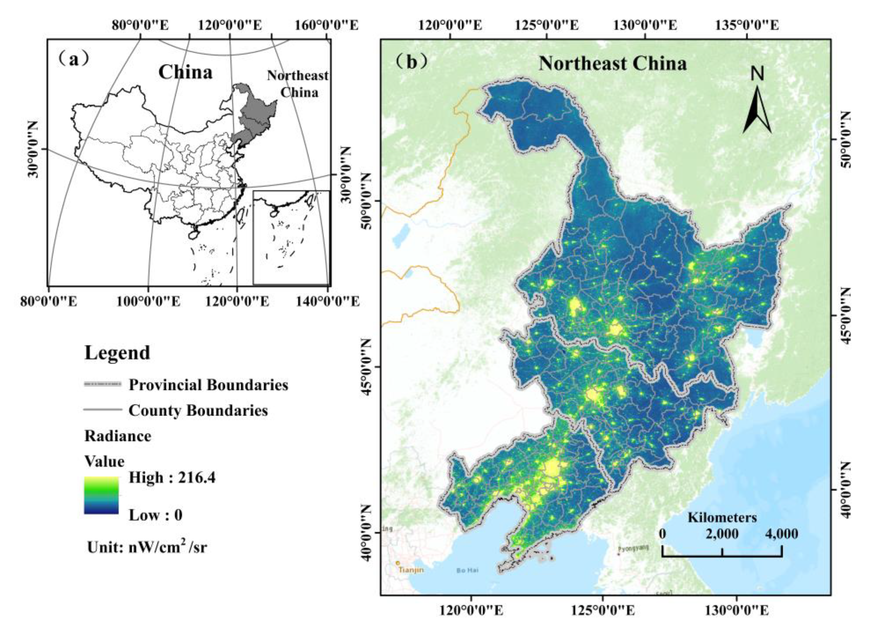
2. Study Area and Datasets
2.1. Study Area
2.2. Datasets
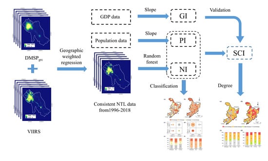
3. Methodology
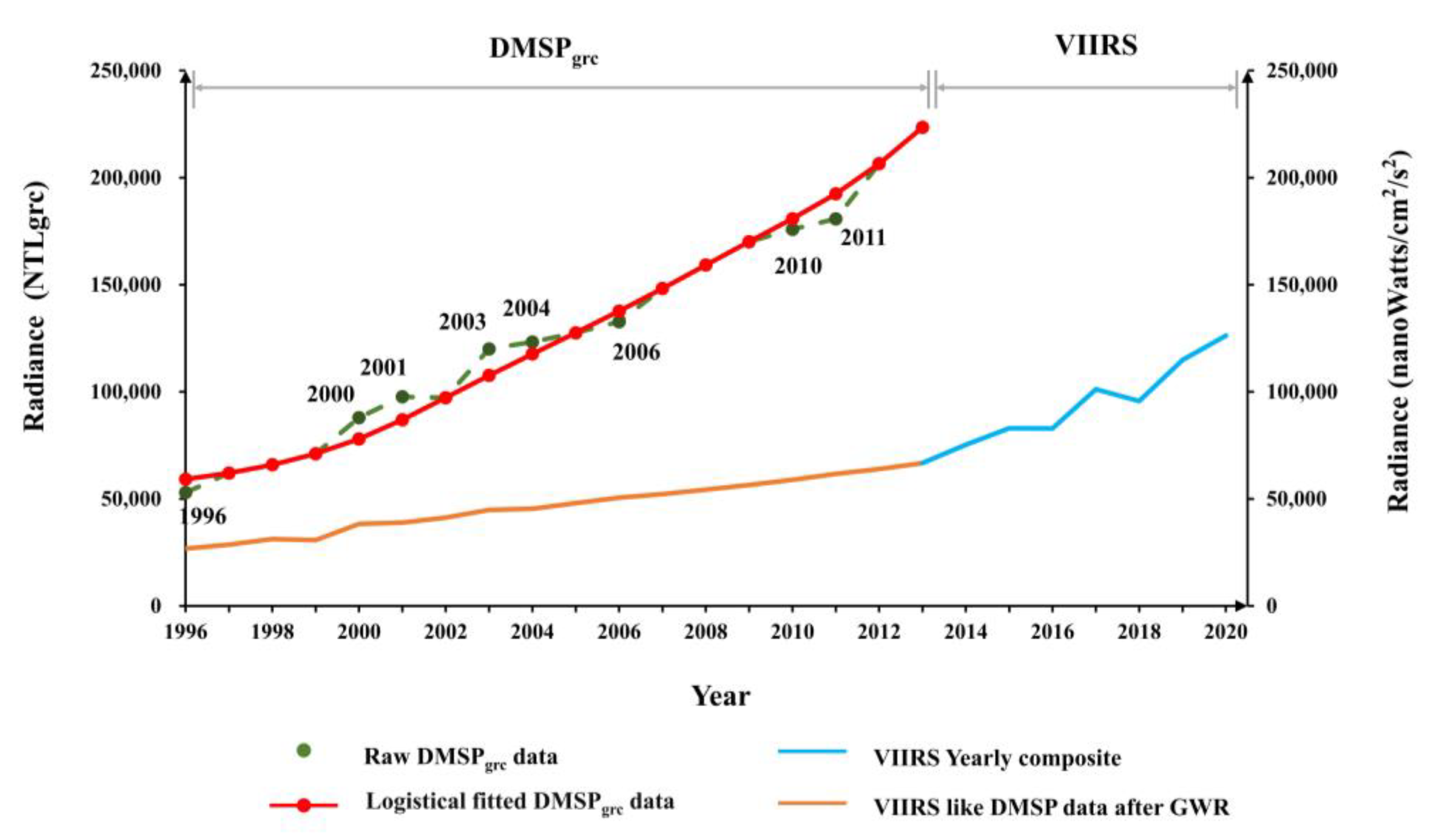
3.1. Data Pre-Processing
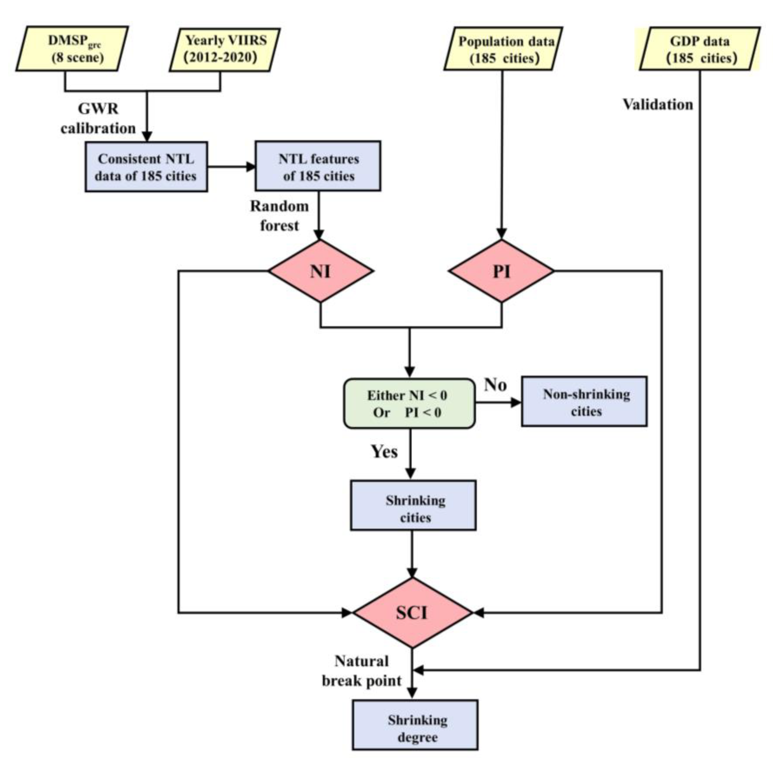
3.2. Construction of the NTL Index (NI) and Population Index (PI)
- (1)
- NTL index (NI)
- (2)
- Population index (PI)
3.3. Shrinking City Classification
4. Results
4.1. Performance Assessment of the Proposed Method
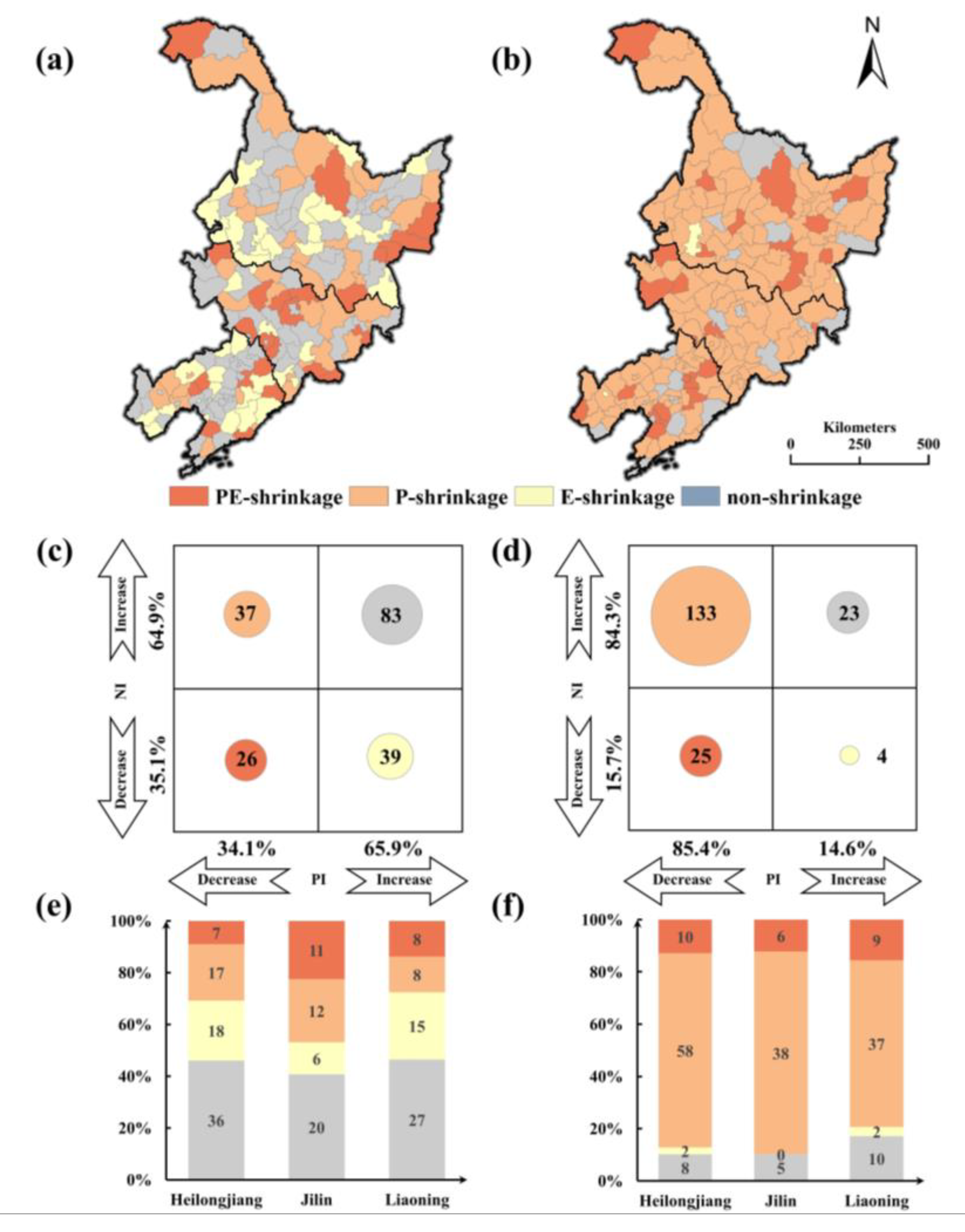
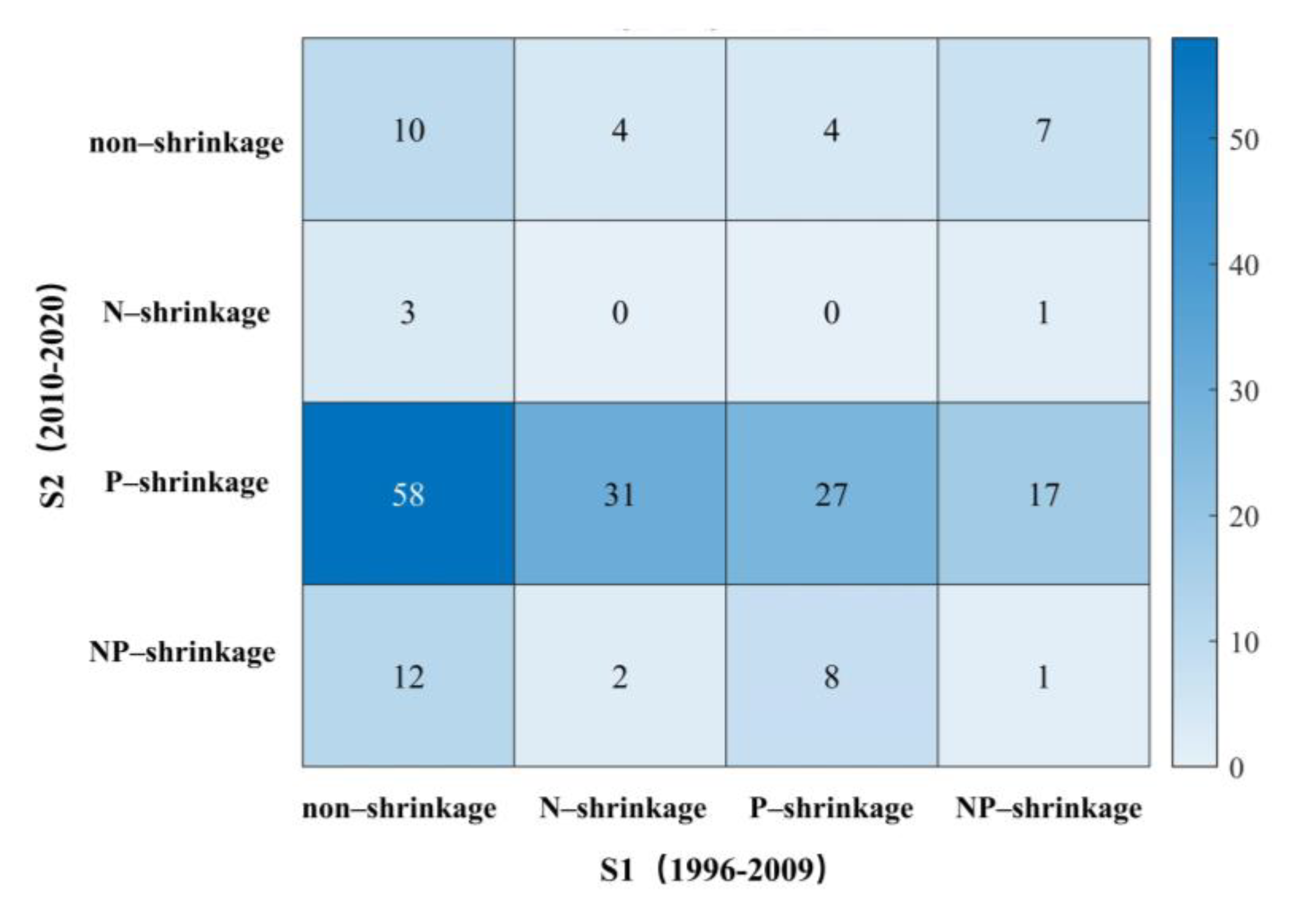
4.2. Spatial Patterns of Shrinking Cities
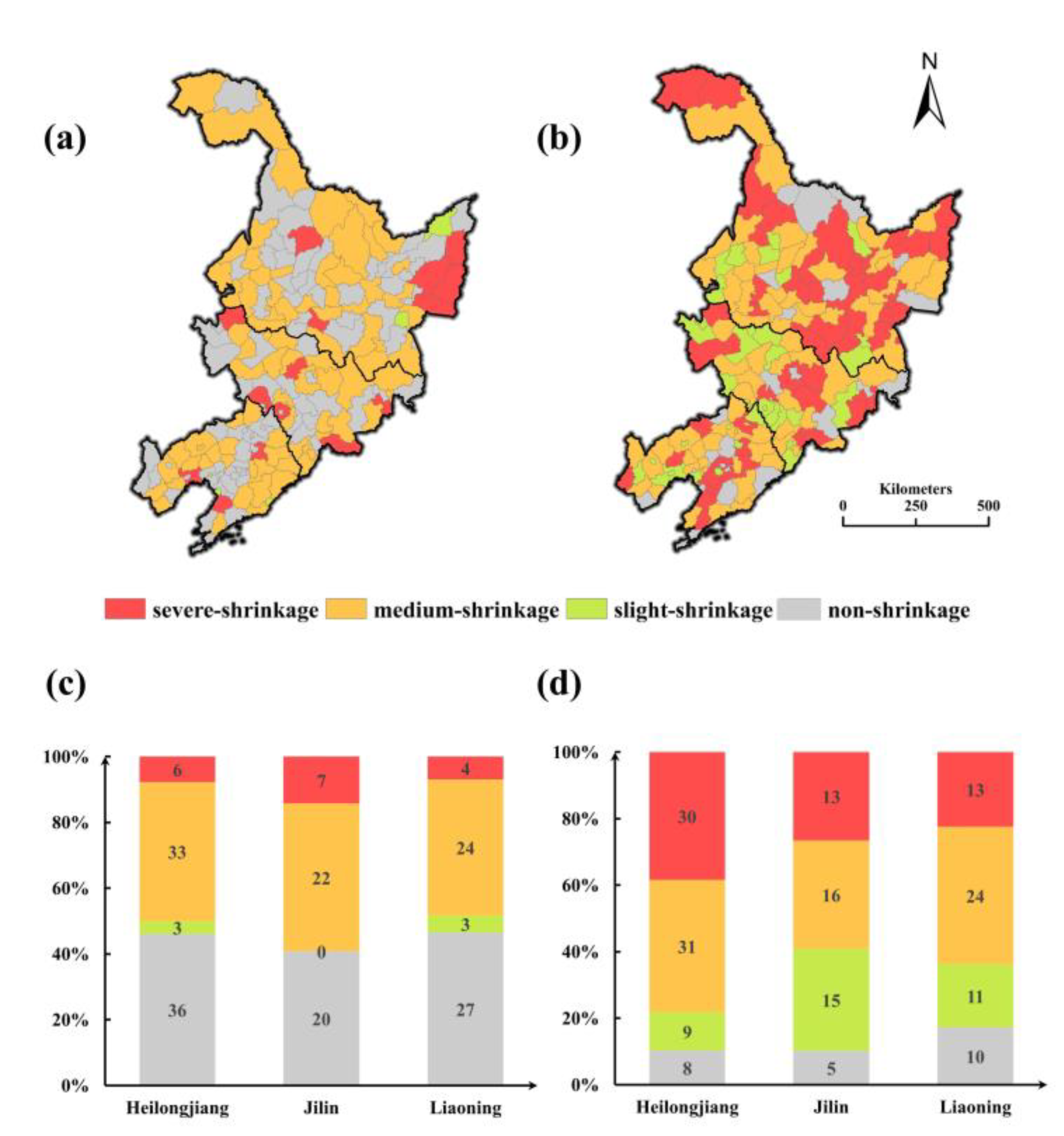
4.3. Degree of Shrinking Cities
5. Discussion
5.1. The Strengths and Limitations of the Proposed Method
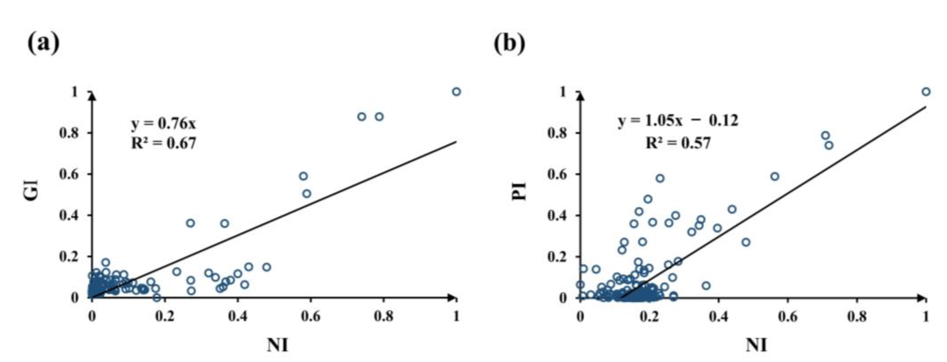
5.2. The Asynchrony of NTL and Population Changes
5.3. Current Situation and Policy Implications
6. Conclusions
Author Contributions
Funding
Institutional Review Board Statement
Informed Consent Statement
Data Availability Statement
Acknowledgments
Conflicts of Interest
References
- Häußermann, H.; Siebel, W. Die Schrumpfende Stadt und Die Stadtsoziologie; Westdeutscher V Erlag: Opladen, Germany, 1988; pp. 78–94. [Google Scholar]
- Wiechmann, T.; Pallagst, K.M. Urban shrinkage in Germany and the USA: A Comparison of Transformation Patterns and Local Strategies. Int. J. Urban Reg. Res. 2012, 36, 261–280. [Google Scholar] [CrossRef]
- Haase, A.; Nelle, A.; Mallach, A. Representing urban shrinkage—The importance of discourse as a frame for understanding conditions and policy. Cities 2017, 69, 95–101. [Google Scholar] [CrossRef]
- Danko, J.J.; Hanink, D.M. Beyond the obvious: A comparison of some demographic changes across selected shrinking and growing cities in the United States from 1990 to 2010. Popul. Space Place 2018, 24, e2136. [Google Scholar] [CrossRef]
- Hattori, K.; Kaido, K.; Matsuyuki, M. The development of urban shrinkage discourse and policy response in Japan. Cities 2017, 69, 124–132. [Google Scholar] [CrossRef]
- Mallach, A. What we talk about when we talk about shrinking cities: The ambiguity of discourse and policy response in the United States. Cities 2017, 69, 109–115. [Google Scholar] [CrossRef]
- Wolff, M.; Wiechmann, T. Urban growth and 3ecline: Europe’s shrinking cities in a comparative perspective 1990–2010. Eur. Urban Reg. Stud. 2018, 25, 122–139. [Google Scholar] [CrossRef]
- Pallagst, K. From urban shrinkage to urban qualities? J. Urban Des. 2019, 24, 68–70. [Google Scholar] [CrossRef]
- Martinez-Fernandez, C.; Weyman, T.; Fol, S.; Audirac, I.; Cunningham-Sabot, E.; Wiechmann, T.; Yahagi, H. Shrinking cities in Australia, Japan, Europe and the USA: From a global process to local policy responses. Prog. Plan. 2016, 105, 1–48. [Google Scholar] [CrossRef]
- Du, Z.; Li, X. Characteristic and mechanism of urban growth and shrinkage from demographic change perspective: A case study of Dongguan. Sci. Geogr. Sin. 2018, 6, 1837–1846. [Google Scholar]
- Du, Z.; Li, X. Growth or shrinkage: New phenomena of regional development in the rapidly-urbanising Pearl River Delta. Acta Geogr. Sin. 2017, 10, 1800–1811. [Google Scholar]
- Long, Y.; Wu, K. Shrinking cities in a rapidly urbanizing China. Environ. Plann. A 2016, 2, 220–222. [Google Scholar] [CrossRef] [Green Version]
- Liu, F.; Zhu, X.; Chen, J.; Sun, J.; Lin, X. The research on the quantitative identification and cause analysis of urban shrinkage from different dimensions and scales: A case study of northeast China during transformation period. Mod. City Res. 2018, 7, 37–46. [Google Scholar]
- Ma, Z.; Li, C.; Zhang, J. Understanding Urban Shrinkage from a Regional Perspective: Case Study of Northeast China. J. Urban Plan. Dev. 2020, 146, 04020027. [Google Scholar] [CrossRef]
- Richardson, H.W.; Nam, C.W. Shrinking Cities: A Global Perspective; Routledge: London, UK, 2014. [Google Scholar]
- Bernt, M. The Limits of Shrinkage: Conceptual Pitfalls and Alternatives in the Discussion of Urban Population Loss. Int. J. Urban Reg. Res. 2016, 40, 441–450. [Google Scholar] [CrossRef]
- Dubeaux, S.; Cunningham Sabot, E. Maximizing the potential of vacant spaces within shrinking cities, a German approach. Cities 2018, 75, 6–11. [Google Scholar] [CrossRef]
- Audirac, I. Introduction: Shrinking Cities from marginal to mainstream: Views from North America and Europe. Cities 2018, 75, 1–5. [Google Scholar] [CrossRef]
- Reis, J.P.; Silva, E.A.; Pinho, P. Spatial metrics to study urban patterns in growing and shrinking cities. Urban Geogr. 2016, 37, 246–271. [Google Scholar] [CrossRef]
- Oswalt, P.; Rieniets, T. Atlas of Shrinking Cities; Hatje Cantz: Ostfildern, Germany, 2006. [Google Scholar]
- Schilling, J.; Logan, J. Greening the rust belt: A green infrastructure model for right sizing America’s shrinking cities. J. Am. Plan. 2008, 4, 451–466. [Google Scholar] [CrossRef]
- Bartholomae, F.; Woon Nam, C.; Schoenberg, A. Urban shrinkage and resurgence in Germany. Urban Stud. 2017, 54, 2701–2718. [Google Scholar] [CrossRef]
- Alves, D.; Barreira, A.P.; Guimarães, M.H.; Panagopoulos, T. Historical trajectories of currently shrinking Portuguese cities: A typology of urban shrinkage. Cities 2016, 52, 20–29. [Google Scholar] [CrossRef] [Green Version]
- He, S.Y.; Lee, J.; Zhou, T.; Wu, D. Shrinking cities and resource-based economy: The economic restructuring in China’s mining cities. Cities 2017, 60, 75–83. [Google Scholar] [CrossRef]
- Khavarian-Garmsir, A.R.; Pourahmad, A.; Hataminejad, H.; Farhoodi, R. Climate change and environmental degradation and the drivers of migration in the context of shrinking cities: A case study of Khuzestan province, Iran. Sustain. Cities Soc. 2019, 47, 101480. [Google Scholar] [CrossRef]
- Döringer, S.; Uchiyama, Y.; Penker, M.; Kohsaka, R. A meta-analysis of shrinking cities in Europe and Japan. Towards an integrative research agenda. Eur. Plan. Stud. 2020, 28, 1693–1712. [Google Scholar] [CrossRef] [Green Version]
- Shan, J.; Liu, Y.; Kong, X.; Liu, Y.; Wang, Y. Identifying City Shrinkage in Population and City Activity in the Middle Reaches of the Yangtze River, China. J. Urban Plan. Dev. 2020, 146, 05020025. [Google Scholar] [CrossRef]
- Olsen, A.K. Shrinking Cities: Fuzzy Concept or Useful Framework? Berkeley Plann. J. 2013, 26, 107–132. [Google Scholar] [CrossRef] [Green Version]
- Shi, K.; Yu, B.; Huang, Y.; Hu, Y.; Yin, B.; Chen, Z.; Chen, L.; Wu, J. Evaluating the Ability of NPP-VIIRS Nighttime Light Data to Estimate the Gross Domestic Product and the Electric Power Consumption of China at Multiple Scales: A Comparison with DMSP-OLS Data. Remote Sens. 2014, 6, 1705–1724. [Google Scholar] [CrossRef] [Green Version]
- Shi, K.; Chen, Y.; Yu, B.; Xu, T.; Yang, C.; Li, L.; Huang, C.; Chen, Z.; Liu, R.; Wu, J. Detecting spatiotemporal dynamics of global electric power consumption using DMSP-OLS nighttime stable light data. Appl. Energy 2016, 184, 450–463. [Google Scholar] [CrossRef]
- Bagan, H.; Borjigin, H.; Yamagata, Y. Assessing nighttime lights for mapping the urban areas of 50 cities across the globe. Environ. Plan. B Urban Anal. City Sci. 2018, 46, 1097–1114. [Google Scholar] [CrossRef]
- Wang, Y.; Huang, C.; Zhao, M.; Hou, J.; Zhang, Y.; Gu, J. Mapping the Population Density in Mainland China Using NPP/VIIRS and Points-Of-Interest Data Based on a Random Forests Model. Remote Sens. 2020, 12, 3645. [Google Scholar] [CrossRef]
- Elvidge, C.; Baugh, K.; Zhizhin, M.; Hsu, F.C.; Ghosh, T. VIIRS night-time lights. Int. J. Remote Sens. 2017, 21, 5860–5879. [Google Scholar] [CrossRef]
- Niu, W.; Xia, H.; Wang, R.; Pan, L.; Meng, Q.; Qin, Y.; Li, R.; Zhao, X.; Bian, X.; Zhao, W. Research on Large-Scale Urban Shrinkage and Expansion in the Yellow River Affected Area Using Night Light Data. ISPRS Int. J. Geo-Inf. 2021, 10, 5. [Google Scholar] [CrossRef]
- Jiang, Z.; Zhai, W.; Meng, X.; Long, Y. Identifying Shrinking Cities with NPP-VIIRS Nightlight Data in China. J. Urban Plan. Dev. 2020, 146, 04020034-1. [Google Scholar] [CrossRef]
- Zhou, Y.; Li, C.; Ma, Z.; Hu, S.; Zhang, J.; Liu, W. Identification of Shrinkage and Growth Patterns of a Shrinking City in China Based on Nighttime Light Data: A Case Study of Yichun. Sustainability 2019, 11, 6906. [Google Scholar] [CrossRef] [Green Version]
- Lang, W.; Deng, J.; Li, X. Identification of “Growth” and “Shrinkage” Pattern and Planning Strategies for Shrinking Cities Based on a Spatial Perspective of the Pearl River Delta Region. J. Urban Plan. Dev. 2020, 146, 05020020. [Google Scholar] [CrossRef]
- Zheng, Q.; Weng, Q.; Wang, K. Developing a new cross-sensor calibration model for DMSP-OLS and Suomi-NPP VIIRS night-light imageries. ISPRS J. Photogramm. 2019, 153, 36–47. [Google Scholar] [CrossRef]
- China Statistical Yearbook; China State Statistics Bureau: Beijing, China, 2012.
- China Statistical Yearbook; China State Statistics Bureau: Beijing, China, 2017.
- Elvidge, C.; Zhizhin, M.; Ghosh, T.; Hsu, F.C. Annual Time Series of Global VIIRS Nighttime Lights Derived from Monthly Averages: 2012 to 2019. Remote Sens. 2021, 13, 922. [Google Scholar] [CrossRef]
- Gong, P.; Li, X.; Zhang, W. 40-Year (1978–2017) human settlement changes in China reflected by impervious surfaces from satellite remote sensing. Sci. Bull. 2019, 64, 756–763. [Google Scholar] [CrossRef] [Green Version]
- Brunsdon, C.; Fotheringham, A.S.; Charlton, M.E. Geographically weighted regression: A method for exploring spatial nonstationarity. Geogr. Anal. 1996, 28, 281–298. [Google Scholar] [CrossRef]
- Breiman, L. Random Forests. Mach. Learn. 2001, 45, 5–32. [Google Scholar] [CrossRef] [Green Version]
- Yang, Y.; Jianguo, W.; Ying, W.; Qingxu, H.; Chunyang, H. Quantifying spatiotemporal patterns of shrinking cities in urbanizing China: A novel approach based on time-series nighttime light data. Cities 2021, 118, 103346. [Google Scholar] [CrossRef]
- Xi, C.; William, N. VIIRS Nighttime Lights in the Estimation of Cross-Sectional and Time-Series GDP. Remote Sens. 2019, 11, 1057. [Google Scholar]
- William, N.; Xi, C. A sharper image? Estimates of the precision of nighttime lights as a proxy for economic statistics. J. Econ. Geogr. 2015, 15, 217–246. [Google Scholar]
- Sun, J.; Di, L.; Sun, Z.; Wang, J.; Wu, Y. Estimation of GDP Using Deep Learning With NPP-VIIRS Imagery and Land Cover Data at the County Level in CONUS. IEEE J. Sel. Top. Appl. Earth Obs. Remote. Sens. 2020, 13, 1400–1415. [Google Scholar] [CrossRef]
- Xie, Y.; Weng, Q. Detecting urban-scale dynamics of electricity consumption at Chinese cities using time-series DMSP-OLS (Defense Meteorological Satellite Program-Operational Linescan System) nighttime light imageries. Energy 2016, 100, 177–189. [Google Scholar] [CrossRef]
- Zhao, M.; Zhou, Y.; Li, X.; Cheng, W.; Zhou, C.; Ma, T.; Li, M.; Huang, K. Mapping urban dynamics (1992–2018) in Southeast Asia using consistent nighttime light data from DMSP and VIIRS. Remote Sens. Environ. 2020, 248, 111980. [Google Scholar] [CrossRef]
- Zhao, N.; Liu, Y.; Hsu, F.; Samson, E.L.; Letu, H.; Liang, D.; Cao, G. Time series analysis of VIIRS-DNB nighttime lights imagery for change detection in urban areas: A case study of devastation in Puerto Rico from hurricanes Irma and Maria. Appl. Geogr. 2020, 120, 102222. [Google Scholar] [CrossRef]
- Gibson, J.; Li, C. The Erroneous use of China’s Population and per Capita Data: A Structured Review and Critical Test. J. Econ. Surv. 2017, 31, 905–922. [Google Scholar] [CrossRef]
- Guan, D.; He, X.; Hu, X. Quantitative identification and evolution trend simulation of shrinking cities at the county scale, China. Sustain. Cities Soc. 2021, 65, 102611. [Google Scholar] [CrossRef]
- Yan, G.; Chen, X.; Zhang, Y. Shrinking cities distribution pattern and influencing factors in Northeast China based on random forest model. Sci. Geogr. Sin. 2021, 41, 880–889. [Google Scholar]
- Ma, Z.; Li, C.; Zhang, J. Characteristics, mechanism and response of urban contraction in Northeast China. Acta Geogr. Sin. 2021, 76, 767–780. [Google Scholar]
- Tong, Y.; Liu, W.; Li, C. Understanding patterns and multilevel influencing factors of small town shrinkage in Northeast China. Sustain. Cities Soc. 2021, 68, 102811. [Google Scholar] [CrossRef]
- Jin, L. Research on the inter-influences between hidden shrinkage of urban population and economic growth—A case study of Maoming in Guangdong Province. J. Harbin Inst. 2018, 1, 133–140. [Google Scholar]
- Sun, J.; Su, X. The strategy of urban smart growth in vied of the revitalization of Northeast China. Soc. Sci. J. 2020, 5, 50–62. [Google Scholar]
- Zheng, Q.; Deng, J.; Jiang, R.; Wang, K.; Xue, X.; Lin, Y.; Huang, Z.; Shen, Z.; Li, J.; Shahtahmassebi, A.R. Monitoring and assessing “ghost cities” in Northeast China from the view of nighttime light remote sensing data. Habitat Int. 2017, 70, 34–42. [Google Scholar] [CrossRef]
- Popper, D.E.; Popper, F.J. Small Can be Beautiful:Coming to Terms with Decline. Planning 2002, 7, 20–23. [Google Scholar]


| Datasets | Periods | Resolution |
|---|---|---|
| DMSPgrc | 1996/2000/2001/ 2003/2004/2006/ 2010/2011 | 30-arc second |
| V2 NPP/VIIRS | 2012–2020 | 15-arc second |
| Population | 1996–2020 | County-scale |
| GDP | 1996–2020 | County-scale |
| Human settlement | 1996–2018 | 30 m |
| Type | S1 (1996–2009) | S2 (2010–2020) | ||
|---|---|---|---|---|
| Low-Speed Expansion | High-Speed Expansion | Low-Speed Expansion | High-Speed Expansion | |
| N-shrinkage | 29 | 10 | 3 | 1 |
| P-shrinkage | 22 | 15 | 76 | 57 |
| NP-shrinkage | 16 | 10 | 16 | 9 |
Publisher’s Note: MDPI stays neutral with regard to jurisdictional claims in published maps and institutional affiliations. |
© 2021 by the authors. Licensee MDPI, Basel, Switzerland. This article is an open access article distributed under the terms and conditions of the Creative Commons Attribution (CC BY) license (https://creativecommons.org/licenses/by/4.0/).
Share and Cite
Dong, B.; Ye, Y.; You, S.; Zheng, Q.; Huang, L.; Zhu, C.; Tong, C.; Li, S.; Li, Y.; Wang, K. Identifying and Classifying Shrinking Cities Using Long-Term Continuous Night-Time Light Time Series. Remote Sens. 2021, 13, 3142. https://0-doi-org.brum.beds.ac.uk/10.3390/rs13163142
Dong B, Ye Y, You S, Zheng Q, Huang L, Zhu C, Tong C, Li S, Li Y, Wang K. Identifying and Classifying Shrinking Cities Using Long-Term Continuous Night-Time Light Time Series. Remote Sensing. 2021; 13(16):3142. https://0-doi-org.brum.beds.ac.uk/10.3390/rs13163142
Chicago/Turabian StyleDong, Baiyu, Yang Ye, Shixue You, Qiming Zheng, Lingyan Huang, Congmou Zhu, Cheng Tong, Sinan Li, Yongjun Li, and Ke Wang. 2021. "Identifying and Classifying Shrinking Cities Using Long-Term Continuous Night-Time Light Time Series" Remote Sensing 13, no. 16: 3142. https://0-doi-org.brum.beds.ac.uk/10.3390/rs13163142