Technical Note

Innovative UAV LiDAR Generated Point-Cloud Processing Algorithm in Python for Unsupervised Detection and Analysis of Agricultural Field-Plots

1
Laboratory of Growth Regulators, Institute of Experimental Botany of the Czech Academy of Sciences & Palacký University, Šlechtitelů 27, 78371 Olomouc, Czech Republic
2
Department of Geoinformatics, Faculty of Science, Palacký University, 17. Listopadu 50, 77146 Olomouc, Czech Republic
3
Department of Chemical Biology, Faculty of Science, Palacký University, Šlechtitelů 27, 78371 Olomouc, Czech Republic
*
Author to whom correspondence should be addressed.
Remote Sens. 2021, 13(16), 3169; https://0-doi-org.brum.beds.ac.uk/10.3390/rs13163169
Submission received: 2 June 2021 / Revised: 2 August 2021 / Accepted: 3 August 2021 / Published: 10 August 2021
(This article belongs to the Special Issue Remote Sensing of Crop Lands and Crop Production)

Abstract

:
The estimation of plant growth is a challenging but key issue that may help us to understand crop vs. environment interactions. To perform precise and high-throughput analysis of plant growth in field conditions, remote sensing using LiDAR and unmanned aerial vehicles (UAV) has been developed, in addition to other approaches. Although there are software tools for the processing of LiDAR data in general, there are no specialized tools for the automatic extraction of experimental field blocks with crops that represent specific “points of interest”. Our tool aims to detect precisely individual field plots, small experimental plots (in our case 10 m 2 ) which in agricultural research represent the treatment of a single plant or one genotype in a breeding trial. Cutting out points belonging to the specific field plots allows the user to measure automatically their growth characteristics, such as plant height or plot biomass. For this purpose, new method of edge detection was combined with Fourier transformation to find individual field plots. In our case study with winter wheat, two UAV flight levels (20 and 40 m above ground) and two canopy surface modelling methods (raw points and B-spline) were tested. At a flight level of 20 m, our algorithm reached a 0.78 to 0.79 correlation with LiDAR measurement with manual validation (RMSE = 0.19 ) for both methods. The algorithm, in the Python 3 programming language, is designed as open-source and is freely available publicly, including the latest updates.
Keywords:
LiDAR; Python; UAV

1. Introduction

Plant growth and development analysis is a key prerequisite for the successful breeding of new varieties and crop research. However, measuring the growth of above-ground plant organs using a “ruler” represents a laborious and rather subjective process as the person performing the measurements cannot measure all the plants in an experimental field plot. This can introduce important bias into the results of the experiment. To overcome these problems methods for the remote sensing of 3D surface modelling are rapidly being developed. In the plant research community “light detection and ranging” LiDAR sensors are being used more and more for what is termed plant phenotyping [1]—a rapidly developing field of plant research technologies aiming at high-throughput and automatic analysis of various parameters of plant growth and physiology. This includes the application of various sensors, but LiDAR has now become the most popular one for the precise estimation of plant height and biomass in field conditions. A boom of methods employing LiDAR can now be observed in agricultural research [2]. LiDAR sensors can be mounted on a tractor-carrier, independent carrying-wheel platform or unmanned air vehicles (UAV) that can be easily applicable in various crops and field-plot designs. A combination of UAV and a LiDAR sensor gives the user the opportunity to make measurements at various locations, independently of field design, the crop species, or their developmental stage. Measuring the plant canopy height using LiDAR was successfully tested in various monocots, showing significant correlations with manually measured parameters. In [3], R 2 = 71.1 was reported in Arundo donax, which is similar to previous results in wheat R 2 = 0.78 [4] or maize R 2 = 0.97 [5]. The accuracy of the measurement is dependent on the object (crop species) being scanned and the scanning and flight parameters. However, the accuracy of the algorithm and the mathematical model used for the estimation of the agronomical characteristics extracted from the point cloud are equally important [5]. The key objectives in point cloud processing for agricultural purposes are: 1. to distinguish points belonging to the crop of interest from those belonging to the ground and also from points that do not represent either of them (typically weeds); 2. to find a model for removing outlier points that arose incidentally during the LiDAR scanning; 3. in the case of a field plot experiment, to detect individual field plots automatically and analyse them as independent experimental units; 4. select a proper model for the expression of spatial information (thousands of points per square metre) in reliable and informative parameters (how the plant height is calculated). After the raw data from the laser scanner is processed, which is usually performed in commercial software, the point cloud file is generated. The next step is to prepare a digital terrain model (DTM), which can also be performed in commercial or open-source software. However, there is a lack of specialized tools for the non-GIS community that can be applied for specific purposes such as crop field plots. As UAV LiDAR sensors become more available and their prices decrease, the need for specific software tools will increase. Specifically, for the estimation of crop height it seems to be useful to design algorithms capable of automatically generating DTM, extracting automatically from DTM points belonging to crops or crop plots and then providing an estimation of crop characteristics such as plant height or biomass. Up to now, most researchers have used non-specific tools for the classification of points within point clouds into the “ground” and “non-ground” classes [3,4,5]. However, for experimental fields that may possibly consist of thousands of field plots some type of automatic processing will be necessary. Here we offer to the community a new software tool in Python programming language that can automatically or semi-automatically process raw point clouds to extract growth parameters, namely canopy height. The goal was to develop end-to-end software purely written in Python without the need of additional software to support our solution. After some research it was obvious that it is a quite challenging goal. There are some public codes of methods for point cloud processing mainly developed in Matlab or C++, but nothing what could provide us with required output. Lack of publicly available tools for point cloud analysis led us to try to develop such a software. This software tool is open-source and is freely available here: https://github.com/UPOL-Plant-phenotyping-research-group/UAV-crop-analyzer, accessed on 1 June 2021.
After the preprocessing steps described in the Material and Methods section, we describe here development of LiDAR processing algorithm that contains following steps: ROI (region of interest) localization module, terrain adjustment, point featurization, classification and edge detection, experimental block localization, plots localization, canopy characteristic extraction. Afterwards, we evaluated LiDAR and algorithm reliability by comparison with manual measurements. Results are summarized in the Discussion and Conclusion section.

2. Materials and Methods

2.1. Field Plot Experiment

For the development of the algorithm, we selected a standard set of five experimental blocks that was not optimized specifically for the UAV LiDAR screening. Although the gaps between the blocks were regularly weeded, during our scanning flight some weeds remained within the gaps intentionally, to demonstrate that the robust algorithm is capable of distinguishing between a field plot with crops and weeds. For our case study, five experimental blocks with 260 plots (each 52 plots) were used. The plot size was 10 m 2 ( 1.15 × 9 m). In all plots, there was winter wheat cv. Turandot (Selgen, Prague, Czech Republic): sowing term: 22 October 2019, sowing rate: 3.5 millions germinated grains, harvesting term: 23 July 2020. The plots were treated with various compounds with the capability of increasing the grain yield (plant growth regulators). Moreover, the field trial showed high differences in plant growth as a result of the non-homogeneous structure of the soil. The UAV LiDAR scanning flights in levels 20 m and 40 m AGL, were performed on 23 June 2020 with time shift between them about 30 min. On the same day as the UAV LiDAR scanning the canopy, height was measured using a manual geodetic measuring bar that was precisely georeferenced by a robotic total station. Five points in one plot were measured, altogether 60 points in 12 plots equally distributed in the first two rows of the experimental block. These manual measures serve for validation of our algorithm. We designed UAV flight plans and set the LiDAR scanning parameters to find some optimal settings for detection crop height as described bellow.

2.2. UAV LiDAR System and Scanning Parameters

Our experimental field-plots were scanned using UAV LiDAR system. The UAV LiDAR system (Ricopter VUX-1UAV, Riegl GmBh, Austria) was operated automatically using the UGCS software (SPH Engineering, Latvia). The flight parameters were planned using the RiPARAMETER software: altitude 20 m and 40 m above ground level (AGL), horizontal speed of flight 4 m·s 1 , scanning line distance 9 m, calculated side overlap ( 77 % , 31 m). The LiDAR sensor was running at the maximum laser pulse rate (550 kHz).

2.3. Pre-Processing of Raw Data

The VUX-1UAV sensor is capable of collecting these types of data: (i) laser data generated by LiDAR; (ii) trajectory data generated by the IMU/GNSS unit, and (iii) images taken by RGB cameras. As we designed our algorithm to be universally applicable to process LiDAR data, RGB images were not collected for this study. The workflow of the data processing is depicted in Figure 1. The first step which has to be performed is to calculate the precise trajectory. The trajectory data are collected by Applanix APX-20 (Trimble Inc., Sunnyvale, CA, USA). IMU/GNSS provides direct georeferencing of airborne sensor data. To increase the precision of the trajectory, the data are further processed with the POSPac UAV software (Trimble Inc., Sunnyvale, CA, USA). The data processing requires correction of the data in RINEX format. Our own GNSS reference station with a RINEX 2.11 format was used. The total RMS error in elevation is below 2 cm. All the other steps of the laser data processing were performed with the RiPROCESS software (RIEGL GmbH, Horn, Austria). Proper settings of “Extraction parameters” include three types of parameters: (i) line angle gate for measurement selection; (ii) deviation gate, and (iii) reflectance gate. All three parameters significantly influence the results. The actual settings are shown in Figure 2.
Three processing parameters have been activated. The first is “Line angle gate for measurement selection“ and this parameter determines swath width for the result. Total swath width in this case is 120 –60 on the left side and 60 on the right side from nadir which has value 180 . The second parameters which has to be set is “Deviation gate“. Due to multiple targets and multiple echoes, deviation occurs in the return pulse. This is caused by targets which are close to each other. Value of 50 was set. All echoes with higher value than 50 is discarded. Deviation does not have unit. The value describes how the pulse shape looks like. Last processing parameters is “Reflectance”. It is an algorithmic ratio which describes the ratio of the actual amplitude of a target to the amplitude of a white flat target at the same range. For example, the reflectance 10 dB means that the target has half reflectance in comparison with white target.
The final point cloud can be visualized in 2D or as a 3D model [1]. Because it is a full waveform scanner, not only one echo but more reflections can be recorded. Before exporting the data, further filtering may be requested. In our case, only points called single targets, first targets, interior or last targets were selected. It means that all points were exported because further analyses (filtration and terrain determining included) were performed in Python. The exporting format was las in version 1.2 and in the UTM Zone 33N projection (EPSG 32633).

2.4. Pre-Processed Data in Raw Format

A las file is an industry-standard binary format for storing airborne LiDAR data. It is an open, binary format specified by the American Society for Photogrammetry and Remote Sensing (ASPRS). The format is widely used and regarded as an industry standard for LiDAR data. For las files manipulation our software uses the Laspy Python library (https://pythonhosted.org/laspy/index.html, accessed on 1 June 2021). The version of las files analysed in this paper is 1.2 (http://www.asprs.org/a/society/committees/standards/asprs_las_format_v12.pdf, accessed on 1 June 2021). A las file generated with a 40 m flight has 9,367,385 points and with a 20 m flight it has 37,506,852 points. The las file of the field that was analysed has 2,730,256 points and a point density of 443 points/m 2 for a 40 m flight. The field for the 20 m flight has 11,456,520 points and a point density of 1895 points/m 2 .

3. Results

3.1. Point Cloud Processing Algorithm

From LiDAR scanning and pre-processing steps (see above) we obtained two files in las format. Two files correspond to different UAV flight levels that we performed to see how the results of scanning are influenced by flight level. Thus, we evaluated LiDAR scanning in 20 m and 40 m above ground level (AGL). Therefore, we tested our algorithm in both point clouds separately. The presented algorithm (Figure 3) in Python 3 programming language provides unsupervised detection of individual block-plots with cereal crop, allowing then easy statistical analysis of crop height. At the beginning, the input las file is cropped to the region of interest (ROI) containing experimental field-blocks with field-plots which growth parameters we wanted to analyze. Subsequently, terrain under the field blocks has to be adjusted to flat enough for later analysis. Afterwards, points of the ground and points of the vegetation are classified using selected features based on neighborhood points. Further, individual experimental blocks are distinguished from the rest of vegetation (e.g., weeds) using newly developed approach of edge detection. Then individual block-plots (experimental plots of area 10 m 2 ) are identified applying Fourier transform. Finally, plant height information, represented by z coordinate of given points in individual block-plots is extracted.

3.1.1. Manual ROI localization Module (Optional)

Usage of first module is optional and depends on scanned area. The purpose of this module is to define rectangular-shape region of interest (ROI) for further analysis. This module visualizes raw point cloud (with a given downsampling rate) and generates a roi_metadata.json file. The user can control visualization with 3 parameters:
  • Downsamplimg rate—determines percentage number of downsampled points of raw point cloud which will be visualized.
  • Low height quantile—determines percentage amount of points with lowest height value, which are not visualized.
  • Up height quantile—determines percentage amount of points with biggest height value, which are not visualized.
Downsampling rate reduces amount of visualized points and can significantly reduces the time of point cloud visualization. Low and Up height quantile remove z-coordinate outliers and improves field visibility. The user defines rectangular-shaped the ROI borders in roi_metadata.json file with arbitrary text editor. The user should define ROI around the experimental blocks tightly so that unnecessary noisy points are not included (see Figure 4).

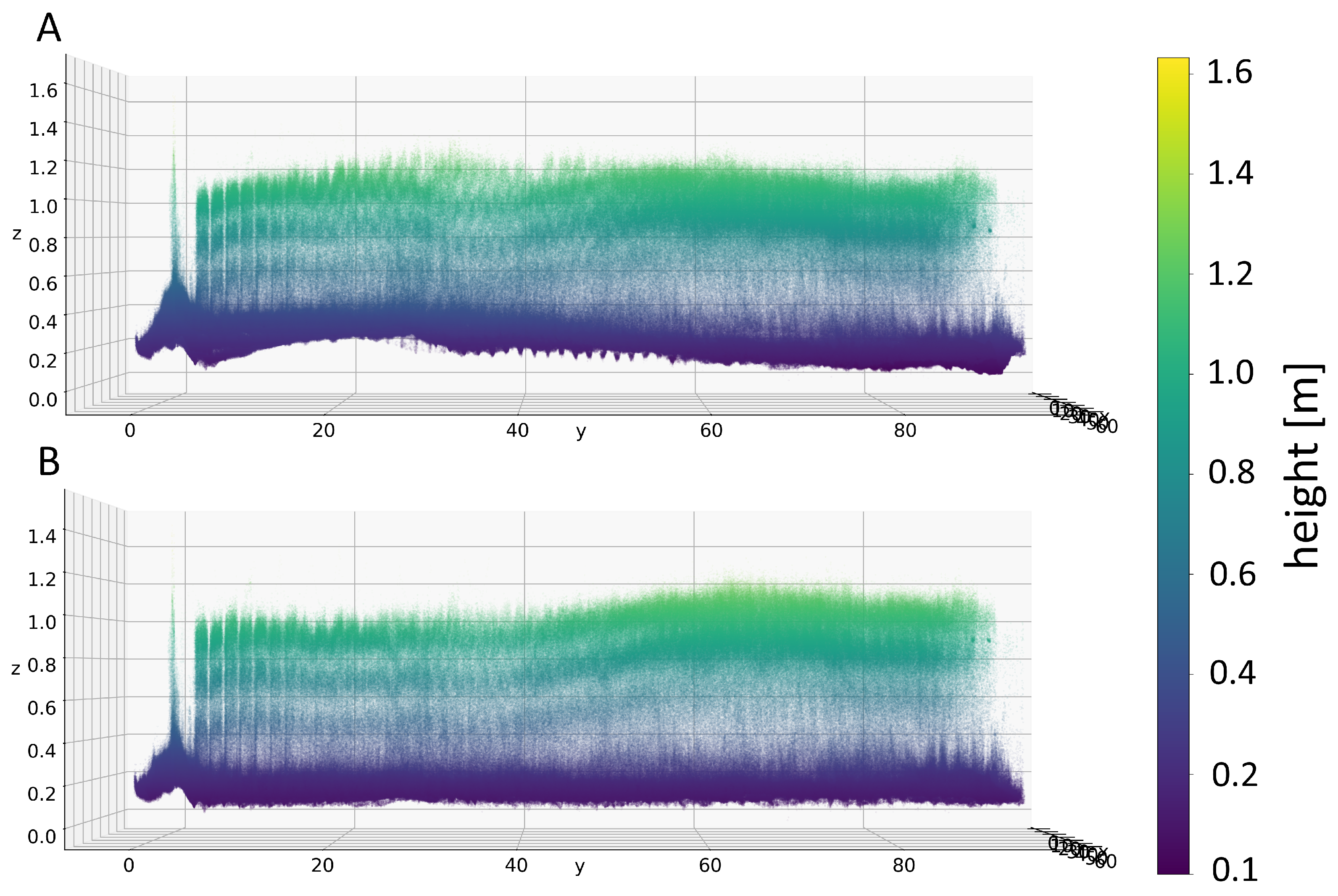
3.1.2. Terrain Adjustment

As the ROI terrain is not naturally flat, it would affect plot growth statistic values. Because of this fact a digital terrain trend removing step was included into the algorithm to remove terrain global trend of ROI. This is performed via the terrain_adjuster.py module. This module performs two essential steps, outliers removal and digital terrain model evaluation and removal. First, outliers are detected and removed from the point cloud. Denoting the ROI point cloud set of points as R, for each point p of R the local neighborhood N given by user-defined radius is determined in the xy-plane with the KDtree algorithm [6] of the scikit-learn Python library. The z-coordinate mean distance d p of point p in its local neighborhood N is determined as,
d p = 1 | N | × n N p z n z , p R .
Then D denotes set of all distances d p and point p is considered as outlier if
d p > μ D + d e v i a n c e × σ D ,
where μ D is mean value of distances D, σ D is the standard deviation value of distances D and deviation is user defined parameter which determines outlier distance significance. An important user-defined parameters for outlier detection are:
  • Metric determines the metric used in the KDtree algorithm and shape of the local neighborhood. Minkowski metric was used in our analysis.
  • Radius defines the size (in meters) of local neighborhood of analyzed point. The radius  0.2 was used in our analysis.
  • Deviance defines how many standard deviations higher than mean distance has to be distance of single point to consider point as outlier. The deviance = 3 was used in our analysis.
After outlier removal cleaned ROI point cloud C is obtained and a clean_roi.las file generated. Further, it is necessary to compute the digital terrain model (DTM) and use it for the terrain effect removal, to allow the measuring of the canopy height and not the effect in the terrain beneath it. This procedure consists of several steps. Points belonging to the terrain are identified by a square sliding window. The window is defined by two parameters size and stride. The window moves around the ROI and in each window area a percentage of points with the lowest z-coordinate value is sampled as “terrain” points with user-defined parameter the window quantile. The size parameter of sliding window is important parameter and has to be determined by user according to shape and size of the experimental blocks. The window size should be big enough, so it cannot happen that in the window will be only points denoting crops. It is recommended to define size of the sliding window so as to be at least as big as the smaller dimension of rectangular-shaped experimental block. The sliding window generates from C points set of the “terrain” points T. As next the regular terrain grid G is formed using T set. In the range ( C x m i n , C x m a x ) and in the range ( C y m i n , C y m a x ) is equidistantly distributed certain number of values. This number is determined with user-defined parameter the grid resolution. Sets of X and Y values are generated and point coordinates in xy-plane of G points are created as
( x , y ) , x X , y Y .
For each point g G , the local neighbourhood N of the k-nearest terrain points of T is determined with the KDtree algorithm and user-defined parameter the K (giving number of nearest neighbours). For each grid point g G its g z coordinate is defined as the z-coordinate mean value of its neighbourhood N. An important parameter of grid is the grid resolution, it determines the density of points in the grid G. Bigger resolution means more detailed and precise estimation of the DTM. The final step of the DTM evaluation is fitting the surface spline to G points using NURBS Python library and generating set of spline points S. Then S points are used to remove the terrain trend of C points. For each c C the closets point in S is evaluated as
argmin s S ( c x s x ) 2 + ( c y s y ) 2 1 2
and set of de-terrained points D t is defined as
d D t : d = ( c x , c y , c z s z ) , c C
The important user-defined parameters for the DTM evaluation and the ROI terrain trend removal:
  • Downsampling rate determines a percentage number of downsampled points which will be processed with module. Since point clouds are huge files in general, to use subset of points can significantly accelerate the computation and decrease processing time.
  • Window size defines the size (in meters) of squared sliding window in xy-plane, which used for terrain points selection. The size of 10 was used in our analysis.
  • Window stride defines how the sliding window is moved around the ROI area. Sliding windows starts in the origin of coordinate system and is moved in xy-plane with given step (in meters). This step is window stride. The stride 1 was used in our analysis.
  • Window quantile defines a percentage of points with lowest value of the z-coordinate in the sliding window, which are selected as the terrain points. In our analysis 0.01  window quantile was used.
  • Metric determines metric used in the KDtree algorithm and shape of the local neighbourhood. Minkowski metric was used in our analysis.
  • K defines the certain number of closest terrain points to given grid point.
  • Grid resolution defines the number of equidistantly distributed points in x axis range and the same number of equidistantly distributed points in y axis range. In the total gird is formed with (grid resolution) 2 points. The value 100 was used for this parameter in our analysis.
  • U degree defines the polynomial order of the spline for first dimension of the parametrical surface space. The value 2 was used in our analysis.
  • V degree defines the polynomial order of the spline for second dimension of the parametrical surface space. The value 2 was used in our analysis.
  • Delta is used to change the number of evaluated spline points. Increasing the number of points will result in a bigger evaluated points array and decreasing will reduce the size of the array. In our analysis delta parameter was configured as 0.01 .
After the model DTM evaluation, the de-terrained set of points D t is generated and exported in the de-terrained_roi.las file (see Figure 5).

3.1.3. Point Featurization, Classification and Edge Detection

The following module of the pipeline, a cloud_evaluator.py performs the point featurization, the ground-crop point classification and the edge points detection. For each point of D t , the neighbourhood of the k-nearest neighbours and the neighbourhood of given radius is determined with the KDTree algorithm. For each neighbourhood, PCA [7] is applied, to compute eigenvalues and eigenvectors. On the basis of computed eigenvalues and eigenvectors, several features are computed (sum of eigenvalues, omnivariance, eigenentropy, anisotropy, planarity, linearity, surface variation, sphericity, verticality, first order moment and average distance in neighbourhood) [8]. It is convenient to use downsampling to reduce the time of processing. It is possible to localize the experimental blocks with even significantly reduced amount of point. After the D t points featurization, two sets of features are generated. F r set for the radius neighbourhood and F k for the k-nearest neighbours neighbourhood. For both sets of features, the Expectation–Maximization clustering using GMM algorithm [7,9] with two components is evaluated. Based on average height of clusters, crop class and the ground class is easily determined for the both clusterings. A point is considered to be crop class only if it was clustered as this class for both feature sets.
To precisely localize the experimental blocks, it is necessary to detect its rectangular-shaped boundaries (see Figure 6). Because of this it seems convenient to try detect edge points in the featurized point cloud. We tried to exploit the existing algorithms for edge point detection in point cloud like [10], but it did not produce nicely structured edges of the experimental blocks. The new method for the experimental block edges detection was developed and it is using result of the clustering from previous step. All D t points are labeled with 0 (ground point) or 1 (crop point). The set of the labels is denoted as L, where
d D t ! l L , l { 0 , 1 } .
To detect the edge point, each labeled point is analyzed on its local neighbourhood N. As a first the k-nearest neighbours in xy-plane are determined with the given metric and K parameters using the KDTree algorithm. Then, neighbourhood N is divided into the two sub-neighbourhoods N + and N using the SVM (Support vector machine) [7] with the linear kernel. Using the labels L as information for the linear SVM supervised training, the optimal separation of N in analyzed point a is given with the plane
p x × ( x a x ) + p y × ( y a y ) + p z × ( z a z ) = 0 .
and n N is determined if it is under N or above N + the plane
p x × ( n x a x ) + p y × ( n y a y ) + p z × ( n z a z ) > 0 n N + p x × ( n x a x ) + p y × ( n y a y ) + p z × ( n z a z ) < 0 n N
The sub-neighborhood of N + and N with the higher amount of crop points ( l = 1 ) is denoted as N c and the second with less crop points as N g . The edge entropy of analyzed point a is defined as
E e = ( 1 + i N g l i ) ( 1 + i N c l i ) × | N c | | N g |
It is expected that on the borders of blocks, plane will separate space in the way that majority of ground points will occur under the plane and majority of crop points above the plane (or opposite). The edge entropy is non-negative and lower the value is, the point is more considered as edge point. The user can determine edge points with parameter entropy quantile which specifies a percentage of points with the lowest value of edge entropy. Important user-defined parameters for the features evaluation and the edge detection are
  • Downsampling rate determines a percentage number of downsampled points which will be processed with the module. Since point clouds are huge files in general, to use the subset of points can significantly accelerate point cloud featurization and decrease processing time. The value 5 % of points was selected for feature evaluation in our analysis.
  • Metric determines metric used in the KDtree algorithm and shape of the local neighbourhood. Minkowski metric was used in our analysis.
  • K defines the k-nearest neighbours neighbourhood of analyzed point. For the feature evaluation 30 neighbours was used and for the edge detection 50 neighbours.
  • Radius defines size (in meters) of the local neighbourhood of analyzed point. The value 0.07 was used for the feature evaluation.
  • Entropy quantile defines a percentage of points with the smallest edge entropy value. These points are considered as the edge points. The value 0.01 was used in our analysis.

3.1.4. Experimental Block Localization

The module block_localizer.py performs the experimental blocks localization. Our method assumes the regular grid of experimental blocks with rectangular shape. First, points classified as crop points L 1 are used for the computation of the optimal point cloud rotation and its orientation. The range of x and y coordinate of L 1 is divided into certain number of intervals with the user-defined signal span parameter which determines the size (in meters) of these intervals. In each interval the mean value of the z-coordinate (the height signal) for the x axis and the y axis is computed and sets of height signals S x and S y are evaluated. For points rotation in the xy-plane, the rotation matrix is defined as
R x y = cos φ sin φ sin φ cos φ
The objective is to find such a rotation φ , which maximizes the height signal variation in the rotated coordinates x and y
argmax 0 < φ < π ( Var ( S x ) + Var ( S y ) )
Then, with the optimal value of φ , the crop points L 1 are rotated into the new coordinate system x y z . The coordinate of x y -plane with the higher value of the height signal variation is defined as dominant and coordinate with the lower value as not-dominant.The experimental blocks orientation is determined with the dominant/not-dominant coordinate evaluation. In this way, the block borders in the rotated coordinate system will be parallel with the x and y axis, so it can be defined with the rectangular-shaped border (see Figure 7A).
Next step is the localization of the experimental block seeds. The block seed is a point which is located within the experimental block border. The height signal with the user-defined signal span parameter, evaluated in the dominant coordinate of the rotated crop points, is used as signal for the seeds localization (see Figure 7B). The seed locations are computed with the Fourier transform [11] as the coordinate of the curve maximum peaks. The user has to specify the number of blocks, which is an essential input for the block localization. Without the correct value it is not possible to localize the experimental blocks.
After the seeds localization in x y -plane the edge points E are rotated into the x y z coordinate system using the R x y rotation matrix and set of rotated edge points is denoted as E . For each analyzed edge point e E two sets of values are defined
ϵ x = { e x : e x w < e x < e x + w } , e E
for the x coordinate and
ϵ y = { e y : e y w < e y < e y + w } , e E
for the y coordinate, where w defines the size of the edge point analyzed area. Based on ϵ x and ϵ y two features for each edge point is computed. The first feature, cardinality is defined as
κ x = | ϵ x | κ y = | ϵ y |
The second feature, uniformity measures the uniformity of the ϵ x values on the ( E x m i n , E x m a x ) interval and the uniformity of the ϵ y on the ( E y m i n , E y m a x ) interval. Kolmogorov-Smirnov (KS) test [12] was used to test uniformity
ϵ x U ( E x m i n , E x m a x ) ϵ y U ( E y m i n , E y m a x ) ,
where U ( E x m i n , E x m a x ) and U ( E y m i n , E y m a x ) denote the uniformly distributed random variables, e E KS test the p-value p x P x and the p-value p y P y are computed.
Uniformity feature is defined as
ν x = p x ( 1 c x ) , ν y = p y ( 1 c y ) ,
where c x is the power of the P x mean value and c y is the power of the P y mean value. The evaluated features cardinality and uniformity are used for the edge point weights θ x and θ y computation which are defined as
θ x = λ × κ x + ( 1 λ ) × ( 1 ν x ) θ y = λ × κ y + ( 1 λ ) × ( 1 ν y ) ,
where λ parameter is the smoothing coefficient defining the mutual significancy of cardinality and uniformity.
The normalized weights Θ x , Θ y of the edge points E and the exp. block seeds are used for the exp. block borders localization. The border rectangular shape is assumed, it means that we need to find [ x m i n , y m i n , x m a x , y m a x ] border values in the x y coordinate system to determine the block location. Denoting single seed as Υ and its area of edge points as
A = { e E : Υ d o m i n a n t ω < e d o m i n a n t < Υ d o m i n a n t + ω } ,
where ω is defined as
ω = 0.45 ( E d o m i n a n t m a x E d o m i n a n t m i n ) # b l o c k s
The range of the x and y coordinates of A are divided into the certain number of intervals with the user-defined signal span parameter which determines the size (in meters) of these intervals. For each interval of the x coordinate, the mean value of Θ x (edge signal) is computed and same for coordinate y and Θ y . Like this set of edge signals, Δ x and Δ y are computed. The seed area A edge signal is divided into the four sub-areas
A x = { δ x Δ x : x < Υ x } A x + = { δ x Δ x : x > Υ x } A y = { δ y Δ y : y < Υ y } A y + = { δ y Δ y : y > Υ y }
Further depending on the exp. blocks orientation, edge signal Δ x and Δ y is reduced to 0 with the user-defined dominant quantile and not-dominant quantile parameters.
δ x A x : δ x < q u a n t i l e q x ( A x ) δ x = 0 δ x A x + : δ x < q u a n t i l e q x ( A x + ) δ x = 0 δ y A y : δ y < q u a n t i l e q y ( A y ) δ y = 0 δ y A y + : δ y < q u a n t i l e q y ( A y + ) δ y = 0 ,
where q x is the quantile value for x axis and q y is the quantile value for y axis.
Based on the exp. blocks orientation, one quantile is dominant quantile and second not-dominant quantile. For the remaining active (positive edge signal) points, stationary points are identified. Point of edge signal point sequence ( x i , δ x i ) is stationary if
δ x i 1 < δ x i δ x i > δ x i + 1
Denoting S x as set of stationary points in A x area, S x + in A x + , S y in A y and S y + in A y + . The block border coordinates are determined as
x m i n = argmin s x : s S x Υ x s x y m i n = argmin s y : s S y Υ y s y x m a x = argmin s x : s S x + Υ x s x y m a x = argmin s y : s S y + Υ y s y
The result of the block localization is saved in the block_metadata.json file. If automatic block localization fails, there is the possibility of defining the block borders manually. The block_manual_check.py module visualizes a top view of the ROI and provides the user with x and y coordinate information via the mouse cursor. In this way, the user can find coordinates of rectangular-shaped borders. This information has to be modified in the block_metadata.json file (via arbitrary text editor modify x m i n , y m i n , x m a x , y m a x attributes of given blocks and save file changes). Important user-defined parameters in block localization module are:
  • Signal span—defines the size of step (in meters) for x and y axis, which is used for the signal computation. A big parameter value is not recommended because it can cause the loss of signal. For the optimal rotation evaluation 0.25 value was used and for the edge signal evaluation 0.01 value was used in our analysis.
  • w—defines the size (in meters) of analyzed edge point area in x or y coordinate. Value 0.1 was used in our analysis.
  • λ —defines the smoothing coefficient defining the mutual significancy of cardinality and uniformity for the edge points weight computation.
  • Dominant quantile—determines the percentage of reduced edge signal values in the dominant coordinate, which are not considered as the candidates for the experimental block border. In our analysis 0.8 value was used.
  • Not-dominant quantile—determines the percentage of reduced edge signal values in not-dominant coordinate, which are not considered as the candidates for the experimental block border. In our analysis 0.98 value was used.

3.1.5. Plots Localization

After the exp. blocks localization, each block is identically analyzed individually. In this step of the processing pipeline we perform localization of the plots in the raw (not de-terrained) block area with the plot_localizer.py module. Again, it is assumed that a single block is made up of a certain number of rectangular-shaped and parallel plots separated by small gaps. The height signal with the user-defined signal span parameter is evaluated in not-dominant coordinate of rotated x y z coordinate system. Plot borders location in not-dominant coordinate is computed with Fourier transform as coordinates of curve minimum peaks (see Figure 8). The user has to specify the number of plots; this is important input for the plot localization. The result of the plot border localization is saved in the block_x_y_metadata.json file, where x and y specify experimental block. An important user-defined parameters for plot localization
  • Signal span—defines the size of step (in meters) in not-dominant coordinate for the height signal computation. Big parameter value is not recommended, it can cause the loss of signal. Value 0.01 was used in our analysis.

3.1.6. Canopy Characteristic Extraction

The last part of pipeline is growth_stats_evaluator.py module which performs the statistic evaluation of growth for each plot (see Figure 9). It analyses a whole batch of plots of a single block and creates a structured result in xlsx format. For the growth analysis only de-terrained rotated points are used. Points of the single exp. block B are cropped from rotated D t with the border coordinates [ x m i n , y m i n , x m a x , y m a x ] and defined as
B = { d D t : ( x m i n < d x < x m a x ) ( y m i n < d y < y m a x ) } .
Single plot P is cropped from the B with the borders in not-dominant coordinate [ τ m i n , τ m a x ] and defined as
P = { d B : ( τ m i n < d n o t d o m i n a n t < τ m a x ) } .
There are two preprocessing steps applied on the plot point cloud P. First, the border area in x y -plane of plot is cropped. This is defined by the user with crop quantile dominant and crop quantile not dominant parameters. The second step is to remove points which have the low height value. These points are not considered as crop points and are filtered out with height quantile parameter.
After the cropping and the low point filtering, cleaned plot point cloud is used for the growth statistic evaluation. There are two ways, how points of cleaned plot are used for statistic evaluation. The first approach evaluates statistics with the raw points of cleaned plot point cloud. The second approach is using surface B-spline. It fits spline to cleaned plot points and evaluate the growth statistics with the surface spline points. Again, Python NURBS library is used for the B-spline fitting. First, regular grid for cleaned plot point cloud is constructed with user-defined grid resolution parameter. The height of each grid point is computed as median of the k-nearest neighbours of cleaned plot points determined with the KDTree algorithm and user-defined K parameter. The spline fitting to the grid points is again configured with the parameters u, v and delta.
The set of the raw features and set of the spline-based features is evaluated. For both approaches 4 growth statistics are evaluated for each plot P. Median of the z-coordinate, variance of the z-coordinate, volume and height expected value. The median is standard 0.5 quantile and the variance is standard sum of squared deviations. The volume is sum of the little blocks defined in x y -plane of plot rectangular area. Blocks fully cover plot area and do not overlap. Blocks have square shape and it’s size is determined by user-defined block size parameter. The height of each block is derived as the median of the z-coordinate in the given block area. The expected value of height is easily determined as the volume divided by plot area.
  • Crop quantile dominant determines a percentage part of the plot area which is removed from plot size in dominant coordinate. It means that half of the crop quantile dominant value is removed from the lower tail and half from the upper tail of the plot dominant coordinate. The reason is to remove noisy borders of plot. Value 0.04 was used in our analysis.
  • Crop quantile not-dominant determines a percentage part of the plot area which is removed from plot size in not-dominant coordinate. It means that half of the crop quantile not-dominant value is removed from the lower tail and half from the upper tail of the plot not-dominant coordinate. The reason is to remove noisy borders of plot. Value 0.3 was used in our analysis.
  • Height quantile filters out from plot point cloud given percentage of points with the lowest value of the z-coordinate. Value 0.2 was used in our analysis.
  • Metric determines metric used in the KDtree algorithm and shape of the local neighbourhood. Minkowski metric was used in our analysis.
  • K defines the k-nearest neighbors of cleaned plot points to the given grid point.
  • Grid resolution defines the number of equidistantly distributed points in the x axis range and the same number of points equidistantly distributed in the y axis range. In total gird is formed with the (grid resolution) 2 points. Value of 100 was used for the plot surface fitting with spline.
  • U degree defines the polynomial order of spline for first dimension of the surface parametrical. Order 2 was used in our analysis.
  • V degree defines the polynomial order of spline for second dimension of the surface parametrical. Order 2 was used in our analysis.
  • Delta is used to change the number of evaluated spline points. Increasing the number of points will result in a bigger evaluated points array and while decreasing will reduce the size of the array. In our analysis delta parameter was configured as 0.01 .
  • Block size defines the size (in meters) of the squared and not-overlaping sliding window, which is sliding around the plot area and is used for the volume computation in the small area of sliding window. The principle of plot volume computation is the same as integration. The volume is the sum of volumes calculated in all sliding window areas in the plot area. In our analysis 0.1 value was used.

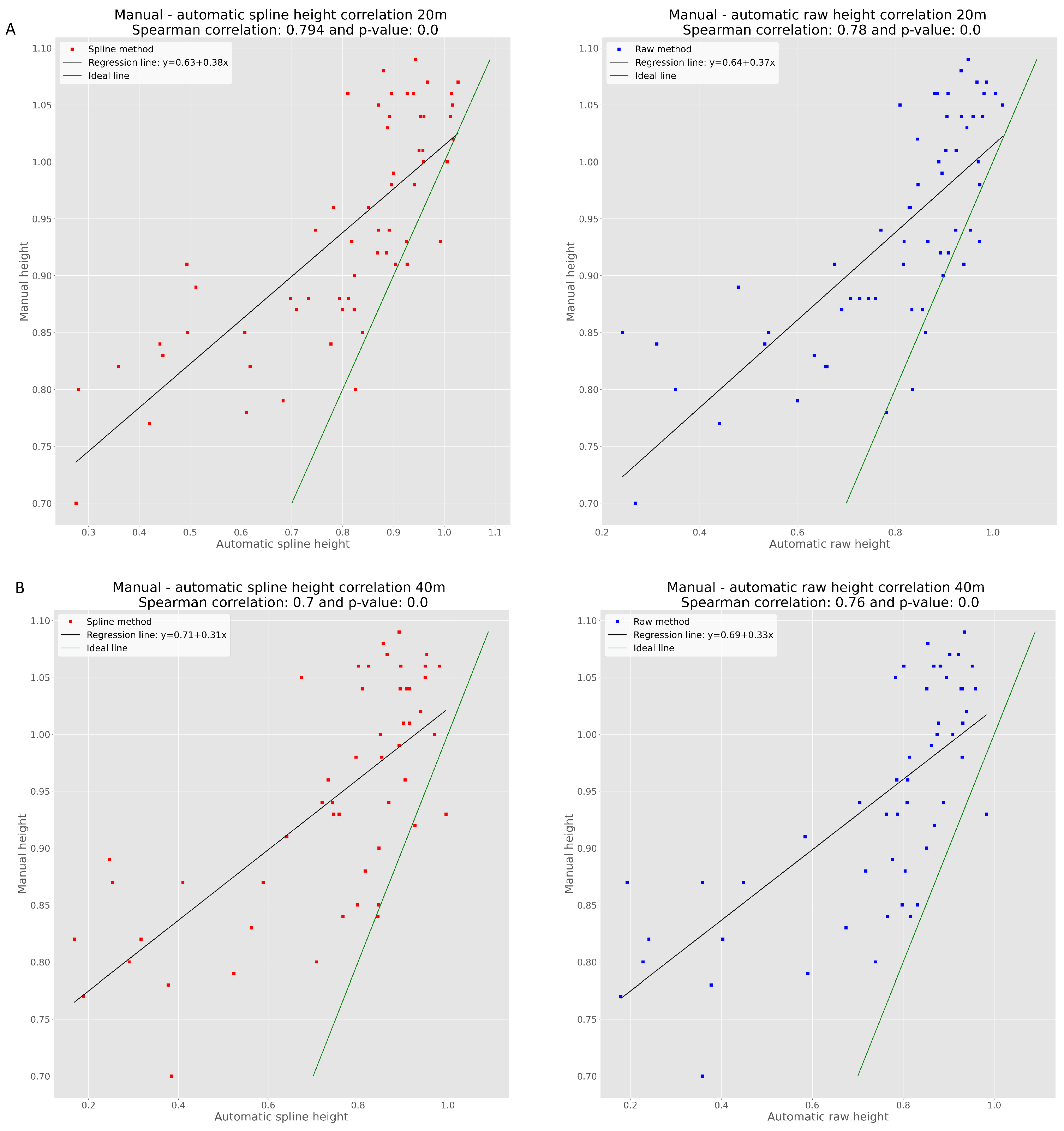
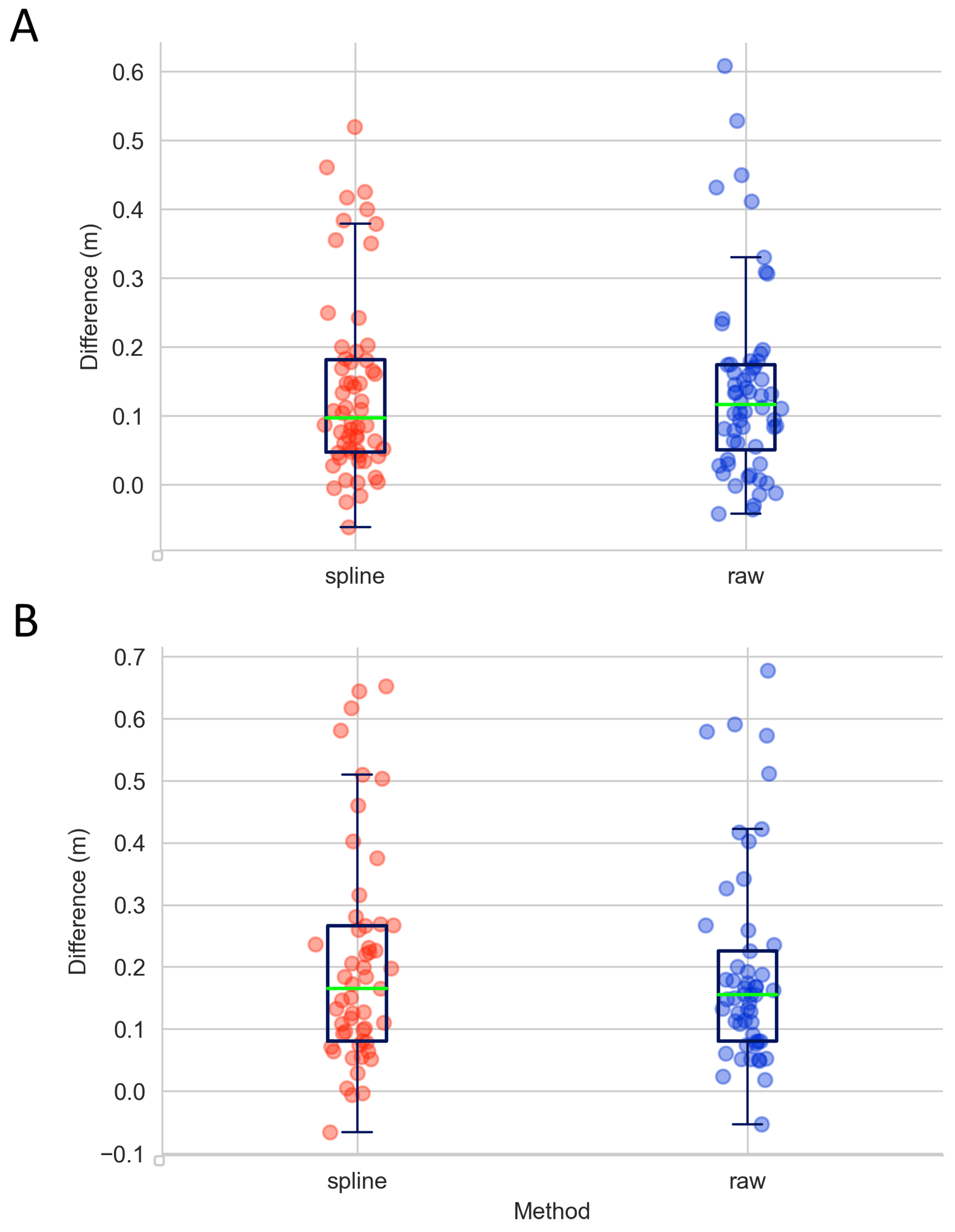
3.2. Validation of Measurements by Manual Measurement of Selected Field-Plots

Our model of canopy height was validated using 60 manually measured points, precisely georeferenced using the total station. It should validate the precision of our canopy height model based on LiDAR measurements. Because of the wind moving the top of the canopy it would not be relevant to compare point-to-point LiDAR measurements directly with manually measured points. For each manually measured point, the relevant neighbourhood was defined as a square with a size of 0.3 m, where the manual point is the centre of the square. The reason for this specific shape is that it is suitable for spline fitting. A neighbourhood point cloud is used to compute a height value representing the automatically measured height of the manual point area. This is done for the raw and spline approaches. Firstly, a low point filtering procedure is applied for a neighbourhood point cloud with the parameter height quantile = 0.2 . The median of the cleaned neighbourhood point cloud z-coordinate expresses the automatically measured height in the area of the given manual point for the raw approach. For the spline method, a surface B-spline has first to be fitted to the cleaned neighbourhood point cloud. A regular grid is constructed with the parameters grid resolution = 10 and K = 1 and a spline with the parameters u,v = 2 and delta = 0.01 . The median of the spline points z-coordinate expresses the automatically measured height in the area of the given manual point for the spline approach. For further analysis there are 60 point-pairs obtained with the 20 m point cloud and 53 point pairs for the 40 m point cloud. The reduction of 7 for the 40 m point cloud is caused by the low density of the scanned/measured points in the manual point area. A minimum limit of three points in a neighbourhood was defined to consider a manual point for validation. However, the size of the square neighbourhood should not be too big and should cover only the area most relevant to the manual measurement.
For 40 m scanning, both methods underestimate the real growth. For the raw method the median of difference (manual-automatic) is 15.5 cm and for the spline method it is 16.5 cm. The median relative/percentage difference is 15.3% for the raw method and 15.6% for the spline method. On the evidence of the boxplot chart, both methods have similar difference distributions. The Spearman correlation coefficient (see Figure 10) was computed to demonstrate the mutual relationship between manual and automatic height measurement (the Pearson correlation coefficient cannot be used because of the violation of the data normality assumption). The raw method correlates with the manual measurements slightly better than the spline method R M S E r a w = 0.251 and R M S E s p l i n e = 0.267 .
For 20 m scanning, both methods also underestimate the real growth. For the raw method the median difference (manual-automatic) is 11.6 cm and for the spline method it is 9.7 cm. The median relative/percentage difference is 12.5 % for the raw method and 9.7 % for the spline method. On the evidence of the boxplot chart (see Figure 11), both methods also have a similar difference distribution for the 20 m scanning. The Spearman correlation coefficient was computed to demonstrate the mutual relationship between manual and automatic height measurement (the Pearson correlation coefficient cannot be used because of the violation of the data normality assumption). The spline method correlates with the manual measurements slightly better than the raw method. However, the difference is even smaller than for 40-m scanning.
Automatic height measurement validation based on manual height measurement shows the opposite results for the raw and spline methods. However, the results do not show big differences. The worse performance of the spline method for 40 m scanning is caused by the lower point density. Fitting the spline to dozens of points in the manual point area in the 40 m point cloud cannot be as precise as fitting it to hundreds of points in the manual point area in the 20 m point cloud. It seems that the raw method is more suitable for low point density scanning and the spline method can be more precise for high point density scanning R M S E r a w = 0.193 and R M S E s p l i n e = 0.192 .

4. Discussion and Conclusions

Our aim in this study was to develop, optimize, and test a software tool for the processing of LiDAR-generated point clouds for the automatic extraction of individual field plots. Individual field plots represent experimental units that are routinely used in field trials by plant breeders and crop researchers. In our case study, we scanned winter wheat field plots growing in very heterogeneous soil by means of a UAV LiDAR sensor in the maximum vegetative growth stage. We designed an algorithm using perhaps most the popular programming language in life science now, Python, to allow reliable analysis of the canopy height, represented by the z-coordinate of a cleaned point cluster belonging to a single field plot. This is reached by a sequence of six steps that allows the modification of the input parameters to optimize algorithm setting for specific data conditions: the number of experimental blocks, number of field plots within the block, terrain slope variations, etc. To see how a different point density will affect the precision of the estimation of the canopy height, we scanned our field trial from two flight levels, 20 and 40 m AGL. We observe that lowering the point density by 77 % (from 1895 to 443 points/m 2 ) led to about a 5 % increase in the difference between the scanned values and those that were manually measured. This suggests that the point density only affects the precision of scanning values to a certain level. This is an important finding on the basis of which we can perhaps find better flight parameters that will be sufficient for scanning precision but do not necessarily generate such dense point cloud data. This is particularly important when we are using a battery-driven UAV whose flying time is considerably limited by the actual battery consumption. The modelling of the canopy surface (the highest layer of the points within the field plot) can affect the parameters that are analysed. We tested two approaches to modelling the canopy surface. Taking only the raw points can certainly be affected by incidental “holes” within the canopy and may not represent the height of the field plot reliably. Here, we worked with the assumption that the plants within one field plot are treated in the same way or represent the same genotype and that their growth parameters should be similar. The differences between plants within one field plot should be smaller than differences between those growing in two different field plots. Thus, taking the raw points only may negatively affect the estimation of real plant growth as understood by plant researchers. For this reason, we also tested a second approach employing the B-spline method, which digitally covers surface points in “cloth”, similarly to what is called the “cloth simulation filter” [13]. This method allows the user to set the parameters of the spline so as to adjust how “dramatic” the surface heterogeneity will be. This may overcome the problem with incidental “holes” in the field plot, but also brings a new risk of inappropriate user input potentially leading to false results. In our case, we set only mild B-spline filtering, resulting in very similar correlations between the values measured with the algorithm and manual validation for both methods, raw and B-spline. In the case of the data generated 20 m AGL, the Spearman correlation coefficient was 0.79 for the B-spline model and slightly lower ( 0.78 ) for the raw points method. This is in agreement with the results of [4], who observed a correlation R 2 = 0.78 in winter wheat using the same UAV LiDAR system as in our study. In the study of [14] in tractor-based LiDAR platform correlation R 2 = 0.9 for wheat was reported. However, there is a question as to how well the manually measured values reflect the true height of the canopy. In our case, the LiDAR values were systematically underestimated in comparison to the manual values. However, it is also possible that the researcher who measured the manual value unintentionally tended to select sampling points that were slightly higher than rest of the field plot, resulting in an overestimated median canopy height. Nevertheless, for field trials the essential feature is usually the relative differences between particular field plots rather than absolute values (see Figure 12). In relative differences any properly optimized sensing method should prevail in accuracy over manual measurements, because it describes the canopy height over the entire plot surface and avoids selective effects introduced by the researcher. However, a multi-seasonal study of field trials will be necessary to verify this assumption. For these reasons, we developed the algorithm presented here, which should serve for easy and reliable point cloud processing for the LiDAR scanning of field trials. The software tool is open-source and freely available in Git-Hub https://github.com/UPOL-Plant-phenotyping-research-group/UAV-crop-analyzer, accessed on 1 June 2021.

Author Contributions

M.P. programmed the mathematical model, generated the visualization of the data, participated in writing the article, and was responsible for the git-hub page with the algorithm. J.M. was responsible for the study design, data collection, pre-processing and generation of input LAS files, and georeferencing of the manual validation, and participated in writing the article. A.E.H. was responsible for data collection and manual validation measurements. Z.Š. was responsible for manual validation measurements and for field trial management. R.K. was responsible for field trial management. J.F.H. initiated the topic and was responsible for data collection and testing and writing the article, and participated in the optimization of the algorithm. All authors have read and agreed to the published version of the manuscript.

Funding

The work was supported from the ERDF project “Plants as a tool for sustainable global development” (No. CZ.02.1.01/0.0/0.0/16_019/0000827).

Institutional Review Board Statement

Not applicable.

Informed Consent Statement

Not applicable.

Data Availability Statement

The software tool presented here is freely available from the github page https://github.com/UPOL-Plant-phenotyping-research-group/UAV-crop-analyzer, accessed on 1 June 2021. The data used in the study is available from the authors upon request.

Conflicts of Interest

The authors declare no conflict of interest.

References

  1. Lin, Y. LiDAR: An important tool for next-generation phenotyping technology of high potential for plant phenomics? Comput. Electron. Agric. 2015, 119, 61–73. [Google Scholar] [CrossRef]
  2. Song, P.; Wang, J.; Guo, X.; Yang, W.; Zhao, C. High-throughput phenotyping: Breaking through the bottleneck in future crop breeding. Crop J. 2021. [Google Scholar] [CrossRef]
  3. Maesano, M.; Khoury, S.; Nakhle, F.; Firrincieli, A.; Gay, A.; Tauro, F.; Harfouche, A. UAV-based LiDAR for high-throughput determination of plant height and above-ground biomass of the bioenergy grass arundo donax. Remote Sens. 2020, 12, 3464. [Google Scholar] [CrossRef]
  4. Ten Harkel, J.; Bartholomeus, H.; Kooistra, L. Biomass and crop height estimation of different crops using UAV-based LiDAR. Remote Sens. 2020, 12, 17. [Google Scholar] [CrossRef] [Green Version]
  5. Luo, S.; Liu, W.; Zhang, Y.; Wang, C.; Xi, X.; Nie, S.; Ma, D.; Lin, Y.; Zhou, G. Maize and soybean heights estimation from unmanned aerial vehicle (UAV) LiDAR data. Comput. Electron. Agric. 2021, 182, 106005. [Google Scholar] [CrossRef]
  6. Bentley, J.L. Multidimensional binary search trees used for associative searching. Commun. ACM 1975, 18, 509–517. [Google Scholar] [CrossRef]
  7. Bishop, C.M. Pattern Recognition and Machine Learning; Springer: Berlin/Heidelberg, Germany, 2006; ISBN 978-0-387-31073-2. [Google Scholar]
  8. Hackel, T.; Wegner, J.; Schindler, K. Contour Detection in Unstructured 3D Point Clouds. In Proceedings of the IEEE Conference on Computer Vision and Pattern Recognition, Las Vegas, NV, USA, 26 June–1 July 2016. [Google Scholar]
  9. Pedregosa, F.; Varoquaux, G.; Gramfort, A.; Michel, V.; Thirion, B.; Grisel, O.; Blondel, M.; Prettenhofer, P.; Weiss, R.; Dubourg, V.; et al. Scikit-learn: Machine Learning in Python. J. Mach. Learn. Res. 2011, 12, 2825–2830. [Google Scholar]
  10. Ahmed, S.M.; Tan, Y.Z.; Chew, C.M.; Mamun, A.A.; Wong, F.S. Edge and Corner Detection for Unorganized 3D Point Clouds with Application to Robotic. In Proceedings of the 2018 IEEE/RSJ International Conference on Intelligent Robots and Systems (IROS), Madrid, Spain, 1–5 October 2018. [Google Scholar]
  11. Bracewell, R.N. The Fourier Transform and Its Applications, 3rd ed.; McGraw-Hill: New York, NY, USA, 1999. [Google Scholar]
  12. Gonzalez, T.; Sahni, S.; Franta, W.R. An Efficient Algorithm for the Kolmogorov-Smirnov and Lilliefors Tests. ACM Trans. Math. Softw. 1977, 3, 60–64. [Google Scholar] [CrossRef]
  13. Millan, V.E.G.; Rankine, C.; Sanchez-Azofeifa, G.A. Crop loss evaluation using digital surface models from unmanned aerial vehicles data. Remote Sens. 2020, 12, 981. [Google Scholar] [CrossRef] [Green Version]
  14. Madec, S.; Baret, F.; De Solan, B.; Thomas, S.; Dutartre, D.; Jezequel, S.; Hemmerlé, M.; Colombeau, G.; Comar, A. High-throughput phenotyping of plant height: Comparing unmanned aerial vehicles and ground lidar estimates. Front. Plant Sci. 2017, 8, 2002. [Google Scholar] [CrossRef] [PubMed] [Green Version]
Figure 1. Workflow of LiDAR data pre-processing.
Remotesensing 13 03169 g001
Figure 2. Extraction parameters for LiDAR data pre-processing.
Remotesensing 13 03169 g002
Figure 3. Novel point-cloud processing algorithm scheme.
Remotesensing 13 03169 g003
Figure 4. Region of interest defined by user.
Remotesensing 13 03169 g004
Figure 5. Terrain profile in an ROI that was analysed (A) before and (B) after terrain adjustment.
Remotesensing 13 03169 g005
Figure 6. (A) Classification of the points; (B) Detection of edge points.
Remotesensing 13 03169 g006
Figure 7. (A) Vegetation points after rotation (experimental blocks are visible in the side view); (B) Fourier transformation of “vegetation point signal” in the dominant coordinate.
Remotesensing 13 03169 g007
Figure 8. Detection of individual field plots using Fourier transformation. (A) Points of single experimental block (front view); (B) Plots border detection using Fourier t.; (C) Borderlines of individual block-plots depicted by the algorithm.
Remotesensing 13 03169 g008
Figure 9. Side view on individual field-plot detected by the algorithm.
Remotesensing 13 03169 g009
Figure 10. Correlation plots of manual measure of plant height with “spline” and “raw methods of automatic plant height estimation” for two UAV flight levels. (A) 20 m AGL; (B) 40 m AGL.
Remotesensing 13 03169 g010
Figure 11. Two methods of computation of plant height (raw and spline) affect the distribution of the difference between LiDAR scanning and manual validation in (A) a 20 m AGL UAV flight and (B) a 40 m UAV flight.
Remotesensing 13 03169 g011
Figure 12. Heat-map visualization depicting canopy height value in an experimental area. Asterisks mark the points of manual validation.
Remotesensing 13 03169 g012
Publisher’s Note: MDPI stays neutral with regard to jurisdictional claims in published maps and institutional affiliations.

