
Class-Wise Fully Convolutional Network for Semantic Segmentation of Remote Sensing Images


1
School of Artificial Intelligence and Automation, Huazhong University of Science and Technology, Wuhan 430074, China
2
School of Computer Science, China University of Geosciences, Wuhan 430074, China
3
School of Mechanical Engineering and Electronic Information, China University of Geosciences, Wuhan 430074, China
*
Author to whom correspondence should be addressed.
Remote Sens. 2021, 13(16), 3211; https://0-doi-org.brum.beds.ac.uk/10.3390/rs13163211
Submission received: 29 June 2021
/
Revised: 10 August 2021
/
Accepted: 11 August 2021
/
Published: 13 August 2021
(This article belongs to the Special Issue Knowledge Graph-Guided Deep Learning for Remote Sensing Image Understanding)
Abstract
:Semantic segmentation is a fundamental task in remote sensing image interpretation, which aims to assign a semantic label for every pixel in the given image. Accurate semantic segmentation is still challenging due to the complex distributions of various ground objects. With the development of deep learning, a series of segmentation networks represented by fully convolutional network (FCN) has made remarkable progress on this problem, but the segmentation accuracy is still far from expectations. This paper focuses on the importance of class-specific features of different land cover objects, and presents a novel end-to-end class-wise processing framework for segmentation. The proposed class-wise FCN (C-FCN) is shaped in the form of an encoder-decoder structure with skip-connections, in which the encoder is shared to produce general features for all categories and the decoder is class-wise to process class-specific features. To be detailed, class-wise transition (CT), class-wise up-sampling (CU), class-wise supervision (CS), and class-wise classification (CC) modules are designed to achieve the class-wise transfer, recover the resolution of class-wise feature maps, bridge the encoder and modified decoder, and implement class-wise classifications, respectively. Class-wise and group convolutions are adopted in the architecture with regard to the control of parameter numbers. The method is tested on the public ISPRS 2D semantic labeling benchmark datasets. Experimental results show that the proposed C-FCN significantly improves the segmentation performances compared with many state-of-the-art FCN-based networks, revealing its potentials on accurate segmentation of complex remote sensing images.
1. Introduction
Semantic segmentation, a pixel-level classification problem, is one of the high-level computer vision tasks. Numerous researchers have investigated the extensions of convolutional neural network (CNN) [1] for semantic segmentation tasks [2,3], because CNN has outperformed traditional methods in many tasks such as image classification [4,5,6], object detection [7,8,9] and image generation [10,11] in the computer vision community. A semantic segmentation network generally retains the feature extraction part of CNN and uses the deconvolution to recover the feature map resolution similar to the size of the input image. A final convolution layer with the size of is applied for pixel-wise labeling to classify every pixel of the last feature map into the corresponding class. Instead of using every patch around each pixel for prediction, semantic segmentation networks based on fully convolutional network (FCN) can efficiently produce pixel-wise predictions. Moreover, global and local relationships of pixels are considered to produce more accurate prediction results with an end-to-end framework.
Segmentation of remote sensing images is a key step for land-use and land-cover classifications, which are crucial in image interpretation and urban mapping [12]. Considering the high resolution and large amounts of remote sensing images, accurate and efficient tools for semantic segmentation are urgently needed. As a result, the deep semantic segmentation networks developed in natural image processing have been noticed and applied in remote sensing image segmentation tasks. FCNs have received increasing attentions in the applications of remote sensing fields because these networks skillfully deal with pixel-wise classification for images of arbitrary sizes and complex textures. Some FCN-based networks have made good progresses on remote sensing image segmentation [13,14,15].
Similar to many deep learning networks, the performance of semantic segmentation networks is highly related to the quality and quantity of training samples. A common phenomenon in practical work is the imbalance of training samples. If samples of one or some classes rarely appear in the training data set, then a deep network could learn limited knowledge of that class. This phenomenon will result in over-fitting problems in the training process and lead to poor generalization capabilities of models. Thus, applications on natural images usually attempt to collect additional samples or augment data by re-sampling or synthesis. These approaches are relatively feasible for natural images. However, using the above schemes on data sets for remote sensing image segmentation is considerably difficult. Substantially imbalanced data problems easily occur in remote sensing segmentation due to the variation of scales of different land-cover categories and man-made objects. Moreover, collecting remote sensing samples of rare classes is often difficult, which indicates that the collection of additional data is not practical for improving the experimental results.
Moreover, existing segmentation networks classify all categories commonly based on the same features extracted by CNN. However, features of categories can be different from each other, especially for remote sensing images. For example, objects in remote sensing images, such as buildings and trees, are quite distinguishable by colors, shapes, and edges. Thus, their features should be distinct for the classifier. By contrast, current segmentation networks only produce general features with a uniform CNN structure and leave all the identification tasks to the last single classification layer. Intuitively, a fine-designed network ought to extract category-specific features in addition to general features. Thus, the model can refine the segmentation results and provide accurate predictions.
Considering the aforementioned issues, a novel network named class-wise FCN (C-FCN) is proposed for remote sensing image segmentation. Inspired by the different characteristics of remote sensing semantic categories and the intuition of category-specific network architecture, various paths for different classes are designed in the proposed network. In this concept, features of each class have their specific flow path, wherein even some difficult or small categories are capable of fitting their model path properly. Consequently, the classifiers will become category-specific ones, which should merely distinguish whether a test sample belongs to one category or not. These binary classifiers will be more concise and dedicated, making them easier to train and fulfill.
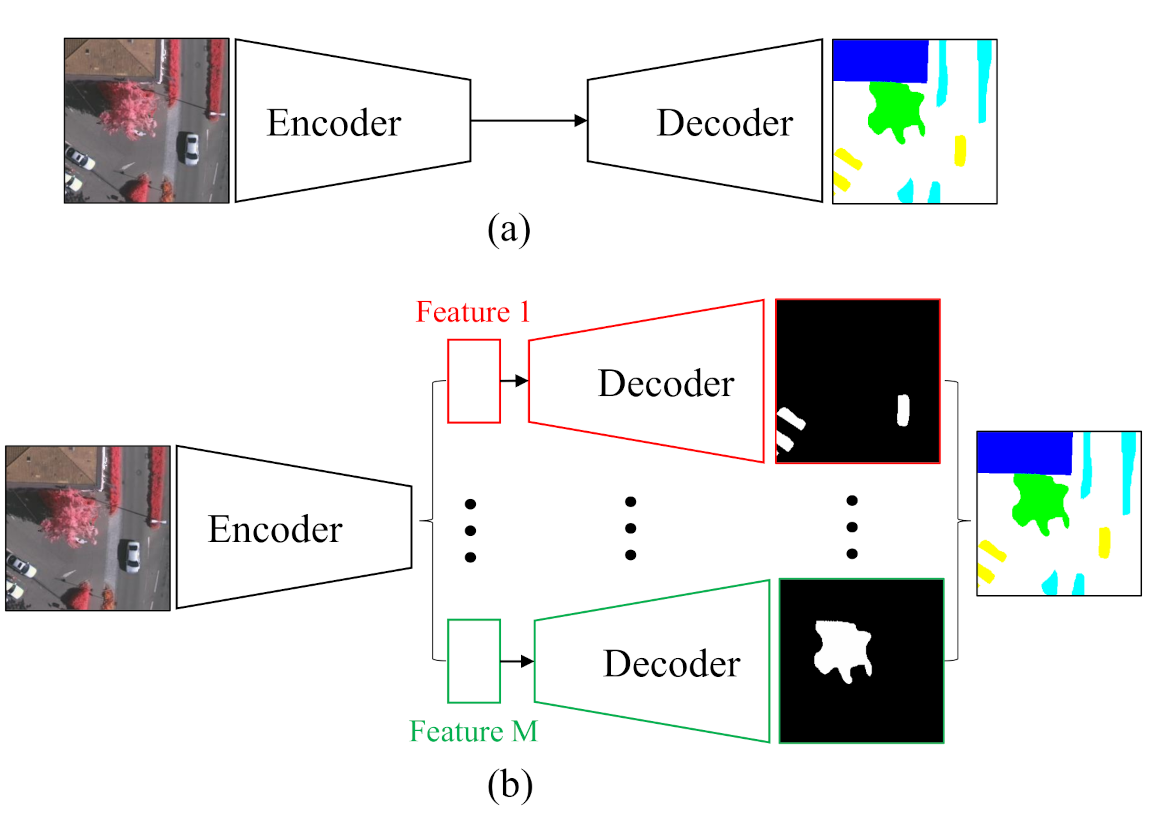
As a typical structure of the current semantic segmentation network, the encoder– decoder structure (Figure 1a) proposed by SegNet [16] has improved the original FCN on the feature map up-sampling method and achieved good performance with dense feature maps. Based on this benchmark network, a straightforward implementation of the above class-wise concept is to run the entire encoder–decoder path for each category in parallel. However, this scheme will suffer from heavy computational costs with the increase of category numbers. Moreover, the repetitive computations of some general features within different classes are unnecessary. Therefore, the proposed network is presented in Figure 1b. In the proposed C-FCN, different classes share the backbone encoder part as much as possible, which extracts general features and reduces the computational burden. Each class possesses an individual decoder and a binary classifier to realize the class-wise feature extraction and specific high-level semantic understanding. In order to achieve the class-wise operation, a class-wise convolution is employed to build our pipeline. Eventually, an end-to-end class-wise network for remote sensing semantic segmentation is obtained by combining all the aforementioned approaches.
It’s widely acknowledged that CNN is a hierarchical network structure, and layers at different levels represent features of different hierarchies. Typically, shallow layers, namely, the layers near inputs, often capture some low-level and simple characteristics of the given image like lines or edges. By contrast, the subsequent layers seize more abstract and high-level features. Hence, skip-connection developed in U-Net [17] is regarded as an essential structure in the building of a segmentation network. Skip-connection reuses the features from former layers to help decoders obtain more accurate segmentation results. In our pipeline, the particularity of the decoder cannot adapt to the original skip-connection structure. Therefore, this part is modified by a newly designed module (class-wise supervision module) such that features and information from the encoder can still skip and flow into the decoders. Meanwhile, the addition of this CS module can help to learn more specific features for each class and boost the realization of class-wise processing.
The main contributions of this paper are concluded as follows.
- An end-to-end network for semantic segmentation of remote sensing images is built to extract and understand class-wise features and improve semantic segmentation performances;
- Based on the above concept, class-wise transition (CT), class-wise up-sampling (CU), class-wise supervision (CS), and class-wise classification (CC) modules are designed in the proposed model to achieve class-wise semantic feature understanding and pixel labeling;
- The network shares the encoder to reduce parameters and computational costs, and the depth-wise convolution and group convolution are employed to realize class-wise operations for each module;
- The proposed model is tested on two standard benchmark datasets offered by ISPRS. Experimental results show that the proposed method has exploited features of most categories and obviously improved segmentation performances compared with state-of-the-art benchmark FCNs.
2. Related Work
2.1. Segmentation Networks
Early in 2015, Long et al. [18] first built an end-to-end network for semantic segmentation by introducing deconvolution into the traditional CNN [4,19,20] pipeline to recover the resolution of feature maps for pixel-wise classification. Since then, a series of work has been conducted to further improve segmentation results by upgrading network structures. U-Net [17] applies skip-connections to all the matching layers in encoders and decoders and adds two convolution layers between skip-connection layers. These modifications enable the decoder to learn gradual up-sampling of feature maps instead of simple interpolation without learnable parameters. SegNet [16] presents a new up-sampling method, in which pooling indexes that store the positions of pooling layers are employed to generate fine segmentation results. DeepLab series [21] proposes several novel concepts such as the átrous convolution, which is implemented by inserting zeros into the convolutional kernels to enlarge the receptive field while preserving parameters constant. PSPNet [22] combines a pyramid module with the existing network for object recognition on different scales. All these fully convolutional networks have made progress on semantic segmentation and provided baseline network structures and useful techniques for the subsequent studies.
After the success of these fully convolutional networks on natural image semantic segmentation, many attempts have been made to transplant them to remote sensing fields. Unlike traditional segmentation methods of remote sensing images that rely on hand-craft features according to specific properties such as spectrums and textures, FCNs combine feature extraction and pixel labeling in a uniform pipeline. Some FCN-based networks have made good progresses on remote sensing image segmentation [13,14,15]. And they have also shown considerable potentials on applications such as building detection [23,24], road extraction [25,26] and instance segmentation [27]. Nevertheless, there is still room for improvements on network architecture due to the complexity and characteristics of remote sensing images.
2.2. Depth-Wise Separable Convolution
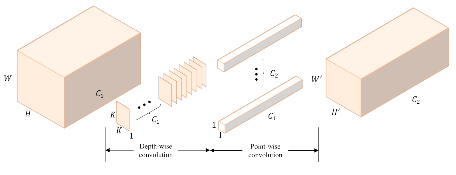
Depth-wise separable convolution has been used in neural network designs since 2014 [28] and has become an essential component in the well-known Xception model [29]. Depth-wise separable convolution can be conducted with the following two parts: a depth-wise convolution, which is a spatial convolution performed independently over each channel of the input; and a point-wise convolution, which is a convolution projecting the output channels by the depth-wise convolution into a new channel space. As shown in Figure 2, depth-wise separable convolution is actually an extreme version of the Inception [30] module.
Depth-wise separable convolution is mainly used in some lightweight networks due to its contribution to parameter reduction. Considering the limited computation resources of mobile devices, networks designed for these platforms can use the depth-wise separable convolution to reduce massive parameters in traditional convolution layers while maintaining reasonable performances. Outstanding representatives that employ depth-wise separable convolution include MobileNet [31] and Xception model [29]. With the development of new lightweight networks such as ShuffleNet [32], a generalized convolution, i.e., the group convolution, has been presented and attracted much attention.
2.3. Group Convolution
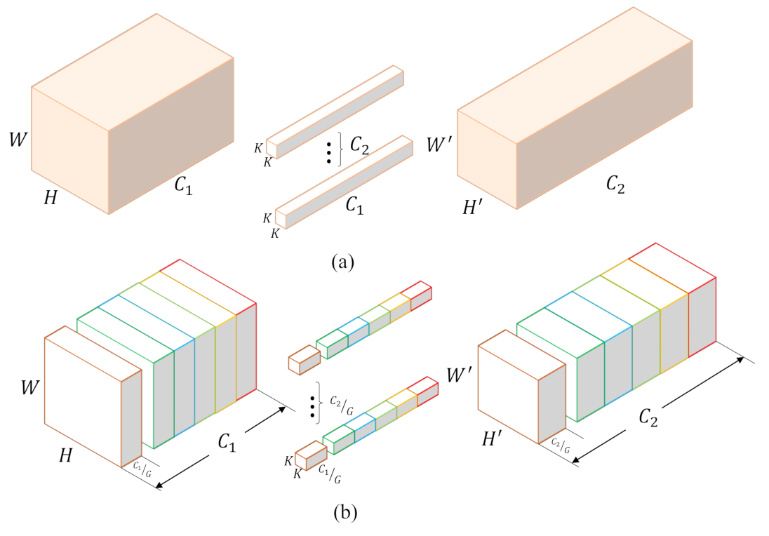
Krizhevsky et al. [4] are the first to use “filter groups” to subdivide the large network AlexNet across two GPUs due to the limited resources. And this trick results in approximately fewer connection weights in network without negative effects on accuracy. Actually, the depth-wise separable convolution can be seen as a special case of the group convolution as shown in Figure 3. The group convolution divides convolution kernels and input channels into several groups, and then convolutes grouped inputs with corresponding kernels. Compared with depth-wise separable convolution in which one feature map is convoluted with one kernel, group convolution uses a group of kernels for the convolution of a group of feature maps. Specifically, suppose that input feature maps have the size of , and the traditional convolution layer has kernels with the size of . In group convolution, feature maps and kernels are divided into G groups on channels. In this case, every grouped kernel only convolutes with feature maps, which means the learnable parameters become , namely, only of the original traditional convolution layer. Therefore, the group convolution can significantly reduce the computational complexity and the number of network parameters.
2.4. Feature Fusion
Skip-connection has become a commonly used structure in segmentation networks [17,18,33], and its superiority has been validated in many researches [34,35]. Conventionally, a skip-connection is built by adding connections between the encoder and decoder, namely, concatenating the features from lower layers to higher ones. The combination of up-sampled features with corresponding features in the encoder will help the decoder to assemble missing information caused by the pooling layers in the encoder, which is hard to recover without skip-connection. The subsequent convolutional layer can then learn to predict the outputs more precisely through the additional information.
Although the naive skip-connection has been employed in many benchmark networks, an increasing number of studies suggest that various designs on skip-connection rather than simple concatenation may be more appropriate for specific applications. In literature [36], researchers add extra convolution block named “boundary refinement” to further refine the object boundaries. Wang et al. [37] use the entropy maps to select adaptive features automatically when merging feature maps in different layers. In literature [38], a network for aerial image segmentation is built by adding extra convolutional layers to merge feature maps back in the up-sampling. All these studies have provided more references for improving the skip-connection architecture in practical applications.
3. Methods
In this paper, we design a novel end-to-end architecture named class-wise fully convolutional network (C-FCN) based on a straightforward idea. Most layers of traditional convolutional neural networks, either for classification or segmentation tasks, concentrate on extracting rich contextual features. Consequently, the classification procedure is left to a few simple convolutional layers or fully connected layers. For example, a segmentation network takes an image with the size of as the input, and obtains the final feature maps f with the size of , then the classification from features to different categories can be formulated as a mapping:
where is the feature vector at position , and M is the number of classes and . It is noticed that all categories are identified by the features in the same space. However, features in a general form may be difficult to classify because categories can be very distinct from each other. Contrarily, if we transform the general features into specific features for different categories, the classification mapping can be decomposed to M mappings of , which will extract more specific features and reduce the classification difficulty.
Based on the above analysis, a straightforward way is to train a convolutional neural network with M paths concurrently, and then merge the outputs to obtain the final segmentation result. However, this scheme will result in a huge number of parameters which lead to expensive training. Therefore, we decide to take the parameter-sharing principle, which means all the M network branches will share one encoding structure. As for the decoder part, we separately decode every class on their own features to share the responsibility of semantic understanding for classifiers. Different from usual convolutional layers, we propose a class-wise convolution to implement all paths within one network.
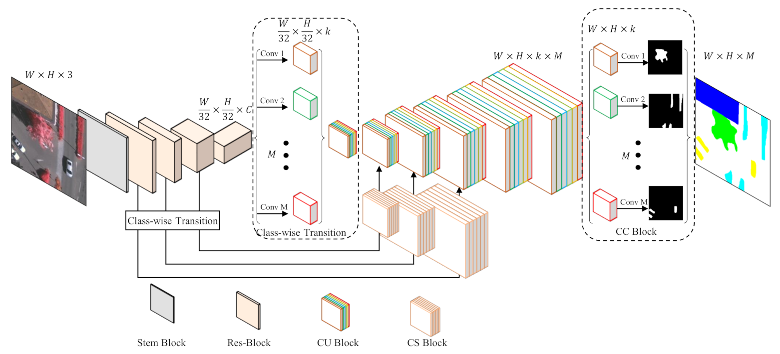
The overall structure of the proposed network is shown in Figure 4. In terms of usual fully convolutional networks, the proposed network can also be parted into two sections: encoder and decoder.
The parameter-sharing encoder can be realized with an arbitrary benchmark network. Considering the performance and affordability, we use the pre-trained ResNet-50, which consists of a Stem Block and four Res-Blocks, as the backbone to extract general features for all categories. Assuming that the input image has the size of , the Stem Block will decrease the feature map size to , and the latter three blocks further downsize the feature maps by a scale of 8. In other words, the stride of the encoder will be 32. Considering the decoder, we customize features for every category by a class-wise transition block (CT), which applies M convolutional layers with k kernels for every category, where M denotes the number of classes and k is a hyper-parameter. By means of this approach, every category is separated to learn how to decode its specific features. Logically, there should be individual decoding paths for M different categories. To keep the network integrated, we design a class-wise up-sampling (CU) block, which is able to decode class-wise features of all classes within one structure by the group convolution. In this case, all categories are actually decoded separately but in a decent form. After five CU blocks, the size of features will be restored to as the original input image. Finally, we use a class-wise classification (CC) block to segment every class based on their specific features.
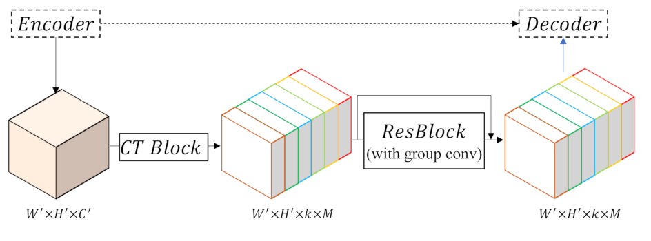
Since skip-connection is one of the most fundamental structures of segmentation networks, we prefer to retain this structure to fuse features from encoder to decoder. However, in our network, features from the encoder are general ones while those from the decoder are class-specific ones, which cannot be simply concatenated. Therefore, we design the class-wise supervision (CS) block to adapt features outflowing from the encoder to facilitate fusion with features in the decoder. Specifically, since CS block bridges the encoder and decoder, it involves the aforementioned Res-Block and CT block.
The four essential components of the proposed C-FCN will be presented in the succeeding sections. Class-wise transition (CT), class-wise up-sampling (CU), class-wise supervision (CS) and class-wise classification (CC) modules are presented in Section 3.1, Section 3.2, Section 3.3 and Section 3.4, respectively, to illustrate their formations and functions.
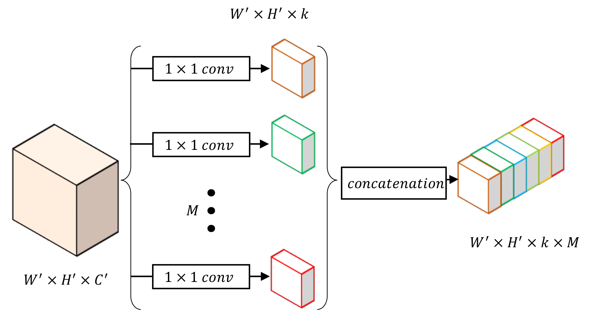
3.1. CT (Class-Wise Transition) Module
In the proposed network, we take ResNet-50 as the encoder, which extracts features of the input image by stacking Res-Blocks. Generally, feature maps from deeper layers are smaller and more abstract than those in shallow layers. All these features, whether deep or shallow, are called “general features” by us, and participate in the classification of all given categories. For the decoder part, the feature extraction and up-sampling path will be split and class-wise processing will be emphasized. In order to transform the general features to class-wise features and link the shared encoder with the class-wise decoder, we design the class-wise transition (CT) block. In brief, the CT block is employed to connect the general structure and the class-wise pipeline. Therefore, the CT block is also applied within the CS blocks besides the junction part between the encoder and decoder.
Figure 5 illustrates the details of a CT block. This module takes general features as the input and uses a convolution layer to facilitate transformation into M class-wise features, where M denotes the number of classes. Moreover, the dimension of every class-wise features is reduced to k during the class-wise convolution to decrease computational cost. After the above convolution, we concatenate the class-wise outputs together on their depth instead of parallel processing of all M features. This specific feature map will then be further processed in CS and CU blocks.
If we keep the same channels for each individual path as the original input, parameters of our network will overload because the class-wise convolution will multiply the channels of the input feature map. Notably, general features are still important in the pipeline, whereas class-wise features only serve individual categories that require relatively less information representation. In the proposed model, channels for each class are reduced by choosing a relatively smaller k than the number of input channel . Experiments will be conducted to evaluate network performance by setting different values of k and verify the scheme.
3.2. CU (Class-Wise Up-Sampling) Module
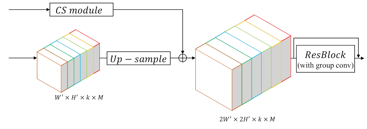
In the traditional FCN [18], after the input image is transformed into highly abstract multi-channel feature maps in the encoder, the decoder will simply recover them to the original size of the input using bilinear interpolation. This implementation is straightforward, but quite rough and not learnable. Instead, we choose UNet [17] as the decoder backbone, which adds a Res-Block after the interpolation layer such that the decoder can learn how to up-sample features. However, in our network, features from the encoder are class-wise, thus we design a class-wise up-sampling (CU) block to build the decoder.
As shown in Figure 4, the decoder includes five CU blocks, and each block will enlarge the feature map twice. Therefore, the final segmentation result can obtain the same resolution as the input image. As explained in the above-mentioned sections, a CT block, which transforms the general features to specific features for each category, emerges before the first CU block. After this transition, all the succeeding convolutions in CU layers should be replaced by group convolution to keep features of every category separated. Moreover, a corresponding CS module will bring in skip features from the encoder for each CU block. The detailed structure of each CU block is shown in Figure 6.
Formally, for one CU block, suppose the input feature map: has the size of , where k is a hyper-parameter, denoting the number of channels for the feature map of each category, and M denotes the number of classes. We first use bilinear interpolation to up-sample the feature map to the size of . Then the up-sampled feature map is added by the output of the corresponding CS module, which will be detailed in Section 3.3. Finally, the feature map is sent into a Res-Block without changing its size, whose output will be the input of the next CU block. After the decoding of five CU blocks, the output feature map will become times larger than the input of the first CU block, which is equal to the original resolution of the input image to be segmented.
3.3. CS (Class-Wise Supervision) Module
Some useful information may be lost as the network goes deep because different levels of CNN capture features of various abstraction levels. Therefore, reusing low level features from the encoder can be very helpful for the decoder to restore more contextual information and obtain improved segmentation result. Formally, the connection between the encoder and decoder is:
where the is the input feature of the layer in the decoder, is its corresponding feature at the encoder, denotes convolution options in the decoder, and represents the set of learnable parameters of the layer.
Though skip-connection fuses features from encoder and decoder to refine segmentation results, features from the two different parts may vary in some respects. Simple and crude fusion with disregard to their differences is inappropriate. Therefore, we add a Res-Block to the path such that features from the encoder can learn how to compensate for the difference and fuse with features in the decoder more appropriately:
Moreover, the skip connection is adapted by adding a CT block on the CS path to fit the proposed model. As shown in Figure 7, taking the general features from the encoder as the input, the CT block will facilitate transformation into class-wise features. A Res-Block is employed to implement class-wise supervision by group convolution, which can be depicted as follows:
where denotes the CT block. As shown in Figure 4, we use three CS blocks, which indicate the presences of three connection paths between the encoder and decoder. Because the first Stem Block in ResNet has a different implementation from the Res-Block, we do not adopt feature fusion on this level.
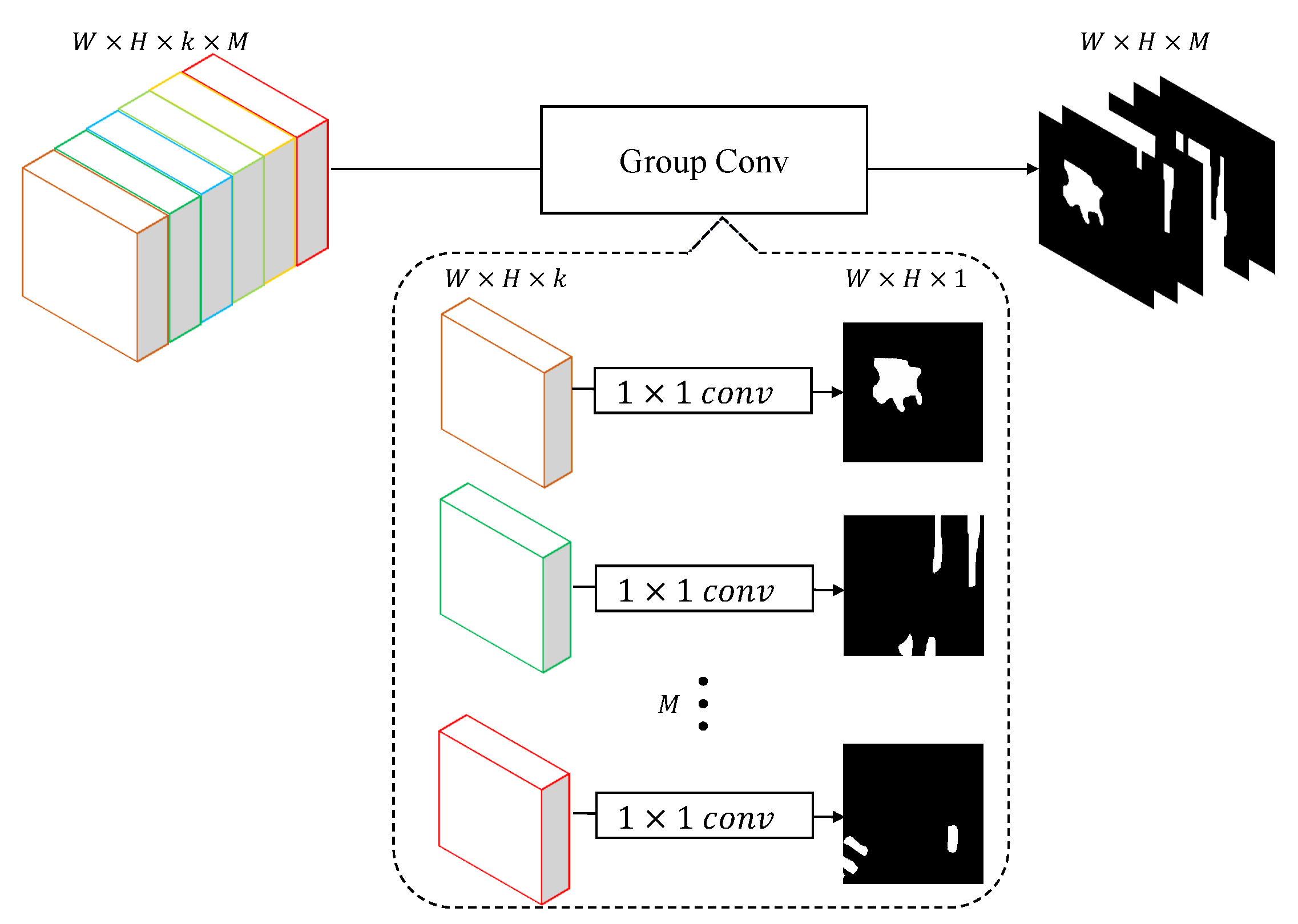
3.4. CC (Class-Wise Classification) Module
In traditional fully convolutional neural networks, the last layer is a convolution layer with the kernel size . A function is then applied to convert the feature vector of each pixel into the probability which presents the likelihood it belongs to a class. In this case, the operation can be defined as:
where is the segmentation result. Since the features output by our model are specific for each class, the classification layer should be class-wise as well. Otherwise, the calculation method of original convolution will hamper the independence between categories. Different from traditional FCNs, the last layer in our C-FCN will be implemented by the group convolution. Details of a CC module are shown in Figure 8. By means of group convolution, the classification module can be regarded as M binary classification layers rather than one M-class classification layer. Let denote the channels of the feature map f, which is a particular feature of class i, and the operation of CC layer in the proposed C-FCN is defined as follows:
where , M denotes the number of classes, denotes the concatenation, and is the probability volume of class belongings. During the training process, is sent to the cross-entropy function for loss calculation. As for segmentation, an function is then employed to identify the class labels.
4. Experiments & Results
4.1. Data Sets
4.1.1. Vaihingen
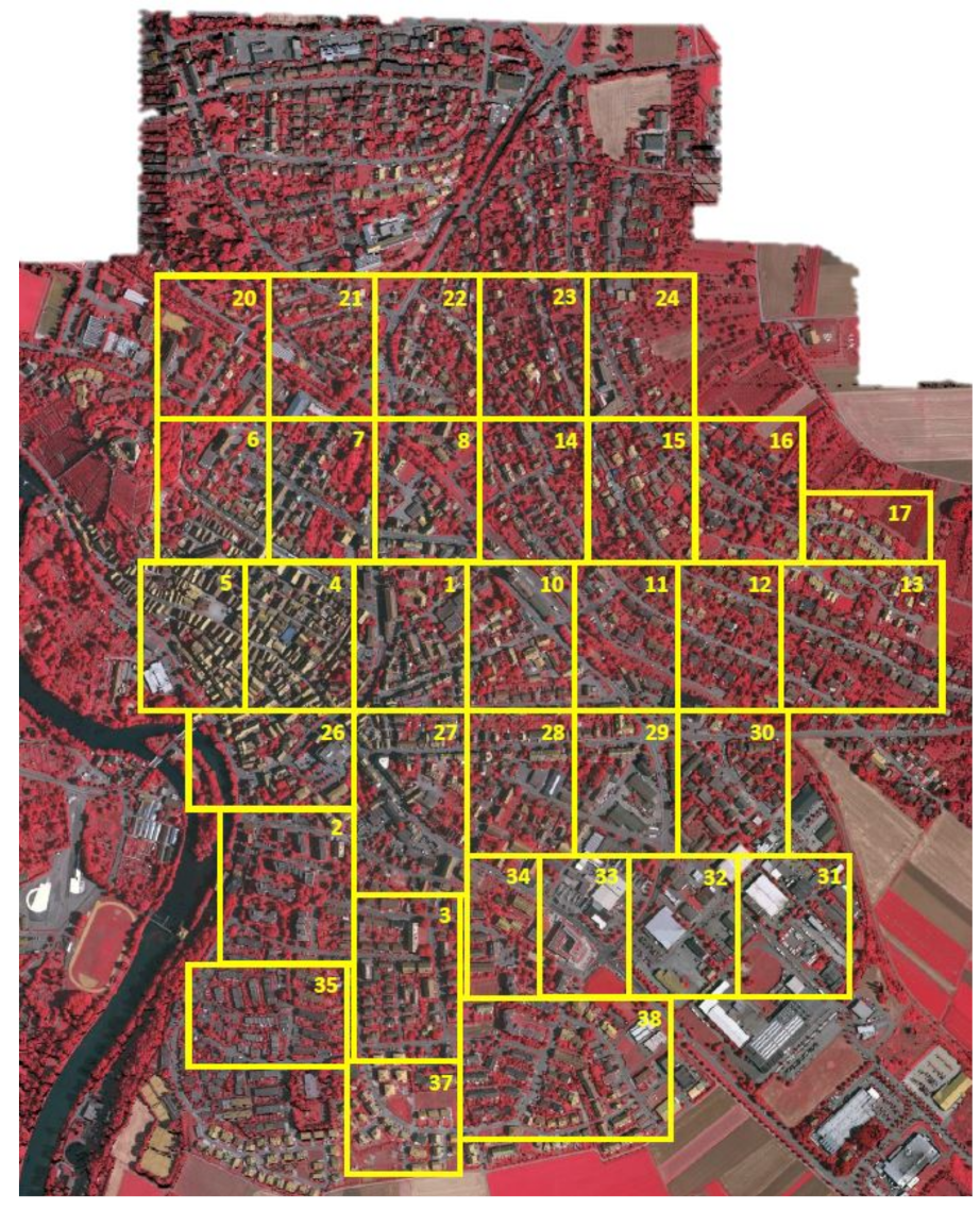
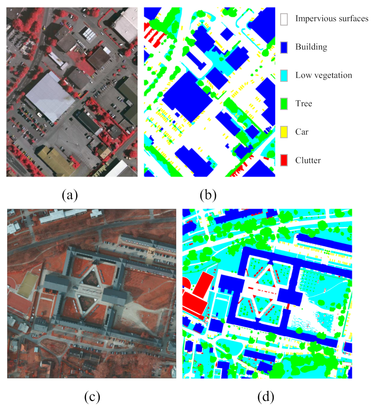
The Vaihingen data set contains 33 tiles (of different sizes), each of which is comprised of a True Ortho Photo (TOP) extracted from a larger TOP mosaic (shown in Figure 9). The ground sampling distance of TOP is 9 cm. All the TOPs are 8-bit TIFF files with three bands, and the RGB channels of the TIFF files correspond to the near-infrared, red and green bands delivered by the camera. The ground truth contains six classes: impervious surface, building, low vegetation, tree, car, and clutter/background, as indicated in Figure 11. As shown in Table 1, all the 33 patches are divided into three sets.
4.1.2. Potsdam
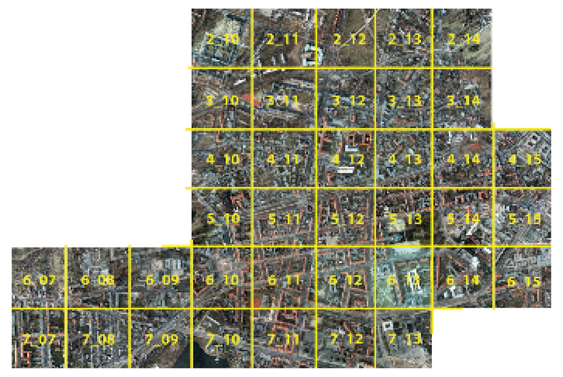
As shown in Figure 10, the Potsdam dataset contains 38 tiles whose ground sampling distance is 5 cm. Unlike Vaihingen dataset, the TOPs of Potsdam come as TIFF files in more channel compositions, which include near-infrared, red, green, blue, DSMs and nDSMs. And each spectral channel has the resolution of 8 bit and DSMs are encoded as 32-bit float values. In consideration of the experiments without changing network structure, we still choose three channels among Potsdam dataset to test our method. Moreover, because both Vaihingen and Potsdam datasets cover urban areas and their land-cover types are similar, we choose RGB channels of Potsdam data to bring in more differences. Similar to Vaihingen dataset, Potsdam dataset has six classes as shown in Figure 11. All patches are divided into three sets as well, which are detailed in Table 1.
4.2. Evaluation Metrics
Two metrics, Intersection over Union (IoU, also named Jaccard Index) and F1-score, are used to evaluate the performances of the proposed model and other baseline models, and their expressions are as follows:
in which,
where, , , and are the true positive, false positive, true negative and false negative, respectively.
4.3. Training Details
All the models, including contrast methods, are implemented on the PyTorch [41] framework. The standard stochastic gradient descent with momentum is chosen as the optimizer to train all the networks and parameters are fixed as recommended: the momentum is 0.9 and the weight decay is 0.0005. The default number of epochs is set to 60, and the training is started with a learning rate of 0.01 which will be multiplied by 0.1 at epoch 5, 10, and 15. Moreover, we monitor the summation of valuation accuracy and F1-score, then early-stop the training when the numeric ceases decreasing. Due to the limit of GPU memory, the batch-size is set to 2∼4 depending on the complexity of models. For models which use ResNet as the backbone, we load weights of encoders pre-trained on ImageNet, while those of the others are initialized with samples from a uniform distribution. In addition, since batch-normalization will not hamper the independence between categories, all the batch-normalization and ReLU functions remain unchanged.
For both data sets, patches are randomly cropped from the training images and then rotated at , and during the training phase. Together with image flips, training sets are finally augmented six times. The validation and test sets do not apply data augmentation. Concretely, 5000 and 7500 patches are respectively cropped on Vaihingen and Potsdam sets. During the test phase, we also crop patches of from each test image with a stride of 128, and stitch them back together after prediction.
4.4. Results & Discussion
This section exhibits the experimental results and analyzes the performances of the proposed network. First, the overall performances of the class-specific design are evaluated to validate the class-wise idea. And then, the usage of the CS module is verified by ablation experiments of two frameworks: one network employs the CS module and the other does not. Moreover, the hyper-parameter k is adjusted in different scales and its different applicable conditions are discussed. Finally, the model is evaluated on the ISPRS 2D semantic segmentation datasets and compared with other state-of-the-art fully convolutional neural networks for segmentation tasks.
4.4.1. Class-Wise Design
Since we take the pre-trained ResNet-50 as the feature extraction backbone and the UNet as the decoder backbone, a backbone network (we mark it as Res-Unet [42]) is formed. Our class-wise network design idea is implemented on this backbone network, so it’s necessary to evaluate the overall performance of the proposed class-wise idea.
As shown in Table 2, results on both datasets of the backbone network Res-Unet and the proposed C-FCN are given. It can be observed that the class-wise design has achieved better results on all Potsdam categories and most Vaihingen categories, which indicate that the inter-class features are better discriminated. Improvements on “clutter” are most evident, which indicate that the class-wise design is beneficial to process hard categories with complex and inapparent within-class features. Results on “tree” and “car” of C-FCN show different tendencies on two datasets. Obvious improvements on Potsdam and slight decreases on Vaihingen can be observed, which may be related to the various band selections of two datasets. Generally, the enhanced average performances of C-FCN can be observed compared to the backbone network. The overall results have validated the effectiveness of the proposed class-wise designing structure.
4.4.2. CS Module
Feature fusion is a very common and useful strategy in semantic segmentation tasks. In our proposed work, due to the modification of the decoder network, we introduce a novel CS module into the traditional skip-connection structure. In order to validate the necessity for class-wise circumstance, an ablation experiment is conducted concerning the CS module.
We test our C-FCN with and without the CS module on Vaihingen dataset, and the results are shown in Table 3. Generally, C-FCN with the CS module outperforms that without the CS module on both F1-score and IoU. More concretely, C-FCN with CS module shows slight advantages on most categories, similar performances on “tree”, disadvantage to some extent on “clutter and background” (as the result is already poor without CS), and tremendous superiority on “car”.
The observations on each category indicate that the employment of the CS module can facilitate the use of features on different levels from the encoder. Accordingly, the detailed information in shallow layers will not be lost by pooling layers and can still be utilized by the decoder. Consequently, the C-FCN is able to recognize small objects and achieve better segmentation results on categories with small samples, as proven by “car”. Results on clutter and background are also interesting and thought-provoking. The use of the CS module is believed to encourage class-specific features and promote class-wise processing. Since this category is relatively special compared with the other classes, which includes all the cluttered land-cover conditions except those five, it may have no “particular features” of its kind for some scenes. Consequently, the addition of CS module in this test under these scenes is not beneficial for the background class, and the emphasis on class particularity even makes the indexes decreased.
4.4.3. Influence of the Hyper-Parameter k
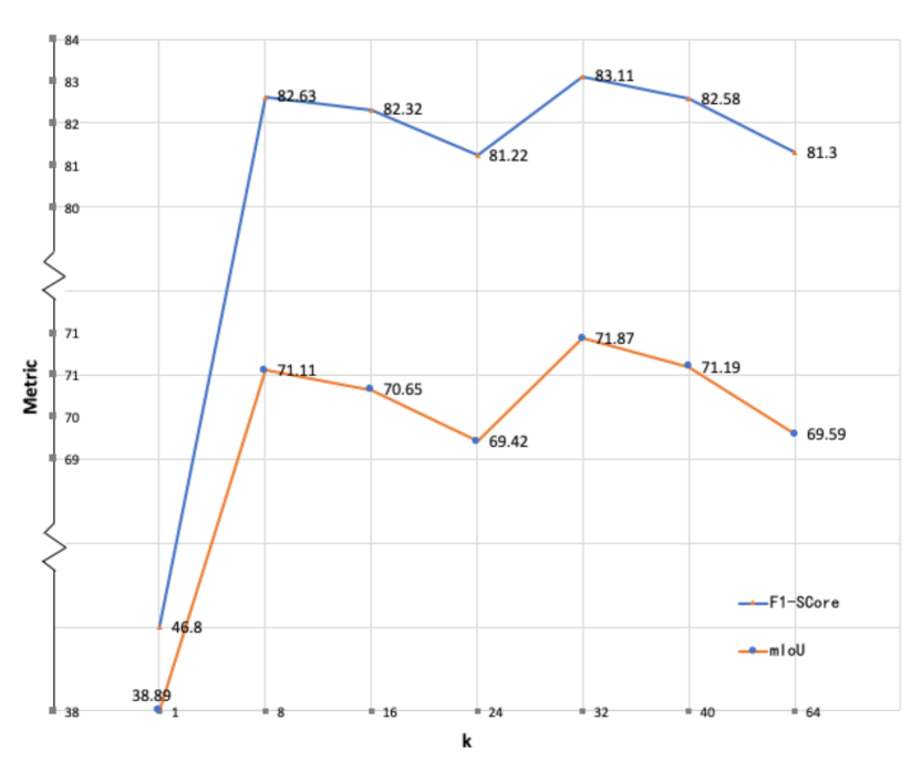
The C-FCN model contains a manually selected hyper-parameter k, which is the number of channels of every class in the feature map. Intuitively, a larger k may be more effective in the model to understand the input image because k is directly related to the number of features of every class. However, recent work [36,43] indicates that an increased number of feature channels may result in limited improvement of final segmentation results. Meanwhile, rapid increase of network parameters will slow down the network training. The proper selection of feature channel numbers is usually based on experiences. Therefore, the model is trained on Vaihingen dataset with different values of hyper-parameter k in ascending orders while other conditions are maintained the same to select an optimal k. Considering representativeness and experiment quantity, k is set to 1, 8, 16, 32, 40 and 64 to observe the performances.
The results are shown in Figure 12. The experiments only cover the range of k from 1 to 64 due to the limitation of GPUs, but this range is thought to be sufficient to reveal a tendency. The figure shows that the F1-score and IoU are fluctuating as k increases. The first peak appears with , and the optimal k equals 32. For better performances within our computational power, we adopt in the method evaluations.
4.4.4. Vaihingen
The proposed C-FCN network is tested on the ISPRS Vaihingen dataset and compared with several baseline and state-of-the-art fully connected networks: (1) FCN [18], the pioneer fully convolutional neural network designed for semantic segmentation; (2) SegNet [16], which has designed an explicit encoder-decoder structure; (3) PSPNet [22], which utilizes the pyramid pooling module to distinguish objects of different scales; (4) Unet [17], which uses concatenations to fuse skip-connection features; (5) Res-Unet, a baseline model we specially build for comparison because it shares a similar backbone structure with our proposed model except for the class-wise designs. All these models are trained on the same partition of datasets and optimized with the same learning rates and decay politics. Limited by the memory of GPU, the batch sizes of models vary from 2 to 4 with regard to the network complexity.
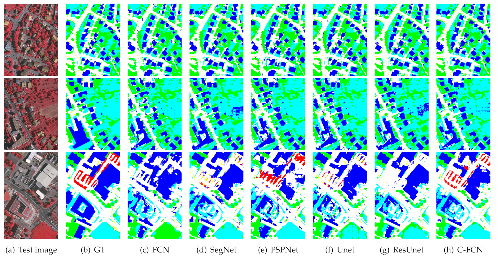
The experimental results are shown in Table 4 and the visualized images are drawn in Figure 13. The numerical results show that our proposed network has a superior overall segmentation performance on this dataset. Since the withered low vegetation is very similar to the rooftop of buildings as shown in the first row of Figure 13, they are easily confused by most networks, even the very deep Res-Unet, while our proposed network performs well on these difficult regions. Though Res-Unet shows very close precision compared with our model because they share a similar network backbone, our proposed network is able to identify the clutter/background class (marked in red) much better than Res-Unet, as shown in the third row of Figure 13. Unlike other classes, the category “clutter” does not have clear entity meaning, which represents those objects excluded from the former five classes. It is seen that most involved networks are insufficient to distinguish these clutters or backgrounds, because these unknown land covers vary a lot on appearances and appear relatively less than other classes. However, a good segmentation framework is required to accurately recognize some uncertain classes as well as the specific land-cover types. The experimental results have shown the potentials of C-FCN on mining features of nonspecific category besides the improvements on specific classes.
4.4.5. Potsdam
The proposed model and the above-mentioned comparison models are also tested on the ISPRS Potsdam dataset, and the training configuration is the same as described in Section 4.4.4. The experimental results are shown in Table 5, from which more obvious advantages of C-FCN can be observed.
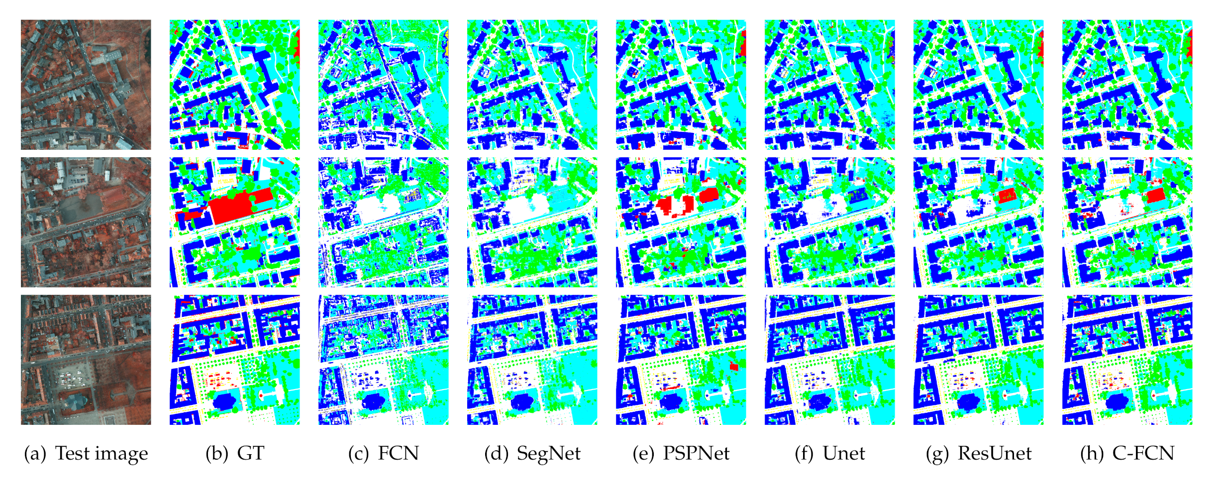
As described in Section 4.1, the Potsdam dataset has a relatively higher resolution compared with that of the Vaihingen dataset, which means we can crop more patches from each training image and obtain more vivid training samples. Particularly, the “clutter/background” category marked in red, appears more frequently in Potsdam dataset. In this case, all the models can better learn information of that category more or less, nevertheless the segmentation results on the test set are still unsatisfying. The results in Table 5 exhibit that the proposed C-FCN still shows better performance on the “clutter/background” category compared with other models. PSPNet outperforms the C-FCN on this category in Vaihingen dataset, but tends to categorize other objects into this class in Potsdam dataset to hamper the IoU when the ground truth areas are actually small (Figure 14, row three). Obvious improvement on “car” category which is marked with yellow is also observed. The car objects are the smallest among all the classes, as a result, this class has small training samples. Accurate segmentation on this kind requires excellent feature extraction on an appropriate scale. And our model outperforms representatives such as PSPNet and Res-Unet, which validates its effectiveness on small scales.
More details can be observed in Figure 14 which reveal that our C-FCN is superior to all the other models on all categories. The segmentation results of SegNet and U-net exhibit numerous miscellaneous points, thus leading to rough edges of buildings. Res-Unet can eliminate most of these tangled points, but as discussed in the Vaihingen dataset, its applicability is limited by the clutter and background categories. On the contrary, C-FCN with specially designed path for every category is capable of distinguishing pixels belonging to background categories more accurately while inheriting the advantages of Res-Unet.
4.4.6. Parameter Size and Inference Time
We have also compared the parameter sizes and inference time of the involved models on the Vaihingen test set including 17 images, as shown in Table 6. GPU time only counts the model inference time while CPU time counts the whole test process. Parameter sizes are measured with MB, and F/B pass indicates the forward/backward pass parameter size. GPU time is shown in seconds and jiffies of CPU time refer to the frequencies of the system. It is seen from the table that the proposed C-FCN has a reasonable amount of parameters compared with other baseline methods. However, its forward/backward pass parameters are much more than the others because of the CT module and group convolutions. As a result, the inference time is slower due to the amount of forward/backward pass parameters. Since the above consumptions are measured under the optimal performance of the network, to balance performance and efficiency, a smaller hyper-parameter k can be concerned to greatly affect the parameter sizes and running time as mentioned in Section 4.4.3.
5. Conclusions
In this paper, we propose a novel end-to-end fully connected neural network for semantic segmentation of remote sensing images. Distinct from traditional FCNs, the class-specific features is believed to play vital roles in semantic segmentation tasks. Therefore, a class-wise FCN architecture is designed to mine class-specific features for remote sensing segmentation. In our pipeline, general features are still captured by a baseline encoder to economize computation, while each class possesses a class-wise skip-connection, a decoder and a classification path through the implementation of class-wise and group convolution. Consequently, a uniform framework is established without the explosion of parameters. We test our framework on ISPRS Vaihingen and Potsdam 2D semantic segmentation datasets. The experimental results have shown remarkable segmentation improvements of the proposed model on most classes, especially on the background class with miscellaneous objects and complex features. In the future work, the class-wise idea on numerous classes with better and faster implementations will be further investigated. If successful, the class-wise segmentation model may possibly be used in more practical remote sensing interpretation tasks and further applied to semantic segmentation of natural images.
Author Contributions
T.T. proposed the idea and wrote the manuscript. Z.C. designed the method pipeline and implemented the validation. Q.H. collected experimental data, solved problems about softwares and helped with validation and visualization. L.M. improved the methodology and edited the manuscript. All authors have read and agreed to the published version of the manuscript.
Funding
This work is supported by the National Natural Science Foundation of China under Grant No. 42071339 and 61771437.
Acknowledgments
The authors would like to thank all the anonymous reviewers for their helpful comments and suggestions to improve the manuscript.
Conflicts of Interest
The authors declare no conflict of interest.
Abbreviations
The following abbreviations are used in this manuscript:
| FCN | Fully Convolutional Network |
| C-FCN | Class-wise Fully Convolutional Network |
| CT | Class-wise Transition |
| CU | Class-wise Up-sampling |
| CS | Class-wise Supervision |
| CT | Class-wise Transition |
| ISPRS | International Society for Photogrammetry and Remote Sensing |
| CNN | Convolutional Neural Network |
| PSPNet | Pyramid Scene Parsing Network |
| TOP | True Ortho Photo |
| RGB | Red Green Blue |
| TIFF | Tag Image File Format |
| DSM | Digital Surface Model |
| IoU | Intersection over Union |
| GPU | Graphics Processing Unit |
References
- LeCun, Y.; Bottou, L.; Bengio, Y.; Haffner, P. Gradient-based learning applied to document recognition. Proc. IEEE 1998, 86, 2278–2324. [Google Scholar] [CrossRef] [Green Version]
- Li, Y.; Shi, T.; Zhang, Y.; Chen, W.; Wang, Z.; Li, H. Learning deep semantic segmentation network under multiple weakly-supervised constraints for cross-domain remote sensing image semantic segmentation. ISPRS J. Photogramm. Remote Sens. 2021, 175, 20–33. [Google Scholar] [CrossRef]
- Ouyang, S.; Li, Y. Combining Deep Semantic Segmentation Network and Graph Convolutional Neural Network for Semantic Segmentation of Remote Sensing Imagery. Remote Sens. 2021, 13, 119. [Google Scholar] [CrossRef]
- Krizhevsky, A.; Sutskever, I.; Hinton, G.E. ImageNet classification with deep convolutional neural networks. In Advances in Neural Information Processing Systems; MIT Press: Cambridge, MA, USA, 2012; pp. 1097–1105. [Google Scholar]
- Yan, J.; Wang, L.; Song, W.; Chen, Y.; Chen, X.; Deng, Z. A time-series classification approach based on change detection for rapid land cover mapping. ISPRS J. Photogramm. Remote Sens. 2019, 158, 249–262. [Google Scholar] [CrossRef]
- Li, X.; Tang, Z.; Chen, W.; Wang, L. Multimodal and Multi-Model Deep Fusion for Fine Classification of Regional Complex Landscape Areas Using ZiYuan-3 Imagery. Remote Sens. 2019, 11, 2716. [Google Scholar] [CrossRef] [Green Version]
- Sermanet, P.; Eigen, D.; Zhang, X.; Mathieu, M.; Fergus, R.; LeCun, Y. Overfeat: Integrated recognition, localization and detection using convolutional networks. arXiv 2013, arXiv:1312.6229. [Google Scholar]
- Tompson, J.; Goroshin, R.; Jain, A.; LeCun, Y.; Bregler, C. Efficient object localization using convolutional networks. In Proceedings of the IEEE Conference on Computer Vision and Pattern Recognition, Boston, MA, USA, 7–12 June 2015; pp. 648–656. [Google Scholar]
- Girshick, R. Fast R-CNN. In Proceedings of the IEEE International Conference on Computer Vision, Santiago, Chile, 7–13 December 2015; pp. 1440–1448. [Google Scholar]
- Ma, J.; Yu, W.; Liang, P.; Li, C.; Jiang, J. FusionGAN: A generative adversarial network for infrared and visible image fusion. Inf. Fusion 2019, 48, 11–26. [Google Scholar] [CrossRef]
- Han, W.; Feng, R.; Wang, L.; Cheng, Y. A semi-supervised generative framework with deep learning features for high-resolution remote sensing image scene classification. ISPRS J. Photogramm. Remote Sens. 2018, 145, 23–43. [Google Scholar] [CrossRef]
- Kang, J.; Fernandez-Beltran, R.; Ye, Z.; Tong, X.; Ghamisi, P.; Plaza, A. Deep metric learning based on scalable neighborhood components for remote sensing scene characterization. IEEE Trans. Geosci. Remote Sens. 2020, 58, 8905–8918. [Google Scholar] [CrossRef]
- Diakogiannis, F.I.; Waldner, F.; Caccetta, P.; Wu, C. ResUNet-a: A deep learning framework for semantic segmentation of remotely sensed data. ISPRS J. Photogramm. Remote Sens. 2020, 162, 94–114. [Google Scholar] [CrossRef] [Green Version]
- Liu, Q.; Kampffmeyer, M.; Jenssen, R.; Salberg, A.B. Dense dilated convolutions’ merging network for land cover classification. IEEE Trans. Geosci. Remote Sens. 2020, 58, 6309–6320. [Google Scholar] [CrossRef] [Green Version]
- Yi, Y.; Zhang, Z.; Zhang, W.; Zhang, C.; Li, W.; Zhao, T. Semantic segmentation of urban buildings from VHR remote sensing imagery using a deep convolutional neural network. Remote Sens. 2019, 11, 1774. [Google Scholar] [CrossRef] [Green Version]
- Badrinarayanan, V.; Kendall, A.; Cipolla, R. SegNet: A deep convolutional encoder-decoder architecture for image segmentation. IEEE Trans. Pattern Anal. Mach. Intell. 2017, 39, 2481–2495. [Google Scholar] [CrossRef]
- Ronneberger, O.; Fischer, P.; Brox, T. U-net: Convolutional networks for biomedical image segmentation. In Proceedings of the International Conference on Medical Image Computing and Computer-Assisted Intervention, Munich, Germany, 5–9 October 2015; Springer: Cham, Switzerland, 2015; pp. 234–241. [Google Scholar]
- Long, J.; Shelhamer, E.; Darrell, T. Fully convolutional networks for semantic segmentation. In Proceedings of the IEEE Conference on Computer Vision and Pattern Recognition, Boston, MA, USA, 7–12 June 2015; pp. 3431–3440. [Google Scholar]
- He, K.; Zhang, X.; Ren, S.; Sun, J. Deep residual learning for image recognition. In Proceedings of the IEEE Conference on Computer Vision and Pattern Recognition, Las Vegas, NV, USA, 27–30 June 2016; pp. 770–778. [Google Scholar]
- Szegedy, C.; Liu, W.; Jia, Y.; Sermanet, P.; Reed, S.; Anguelov, D.; Erhan, D.; Vanhoucke, V.; Rabinovich, A. Going deeper with convolutions. In Proceedings of the IEEE Conference on Computer Vision and Pattern Recognition, Boston, MA, USA, 7–12 June 2015; pp. 1–9. [Google Scholar]
- Chen, L.C.; Papandreou, G.; Kokkinos, I.; Murphy, K.; Yuille, A.L. Deeplab: Semantic image segmentation with deep convolutional nets, atrous convolution, and fully connected CRFs. IEEE Trans. Pattern Anal. Mach. Intell. 2017, 40, 834–848. [Google Scholar] [CrossRef]
- Zhao, H.; Shi, J.; Qi, X.; Wang, X.; Jia, J. Pyramid scene parsing network. In Proceedings of the IEEE Conference on Computer Vision and Pattern Recognition, Honolulu, HI, USA, 21–26 July 2017; pp. 2881–2890. [Google Scholar]
- Shahzad, M.; Maurer, M.; Fraundorfer, F.; Wang, Y.; Zhu, X.X. Buildings Detection in VHR SAR Images Using Fully Convolution Neural Networks. IEEE Trans. Geosci. Remote Sens. 2019, 57, 1100–1116. [Google Scholar] [CrossRef] [Green Version]
- Ji, S.; Wei, S.; Lu, M. Fully Convolutional Networks for Multisource Building Extraction From an Open Aerial and Satellite Imagery Data Set. IEEE Trans. Geosci. Remote Sens. 2019, 57, 574–586. [Google Scholar] [CrossRef]
- Yang, X.; Li, X.; Ye, Y.; Lau, R.Y.K.; Zhang, X.; Huang, X. Road Detection and Centerline Extraction Via Deep Recurrent Convolutional Neural Network U-Net. IEEE Trans. Geosci. Remote Sens. 2019, 57, 7209–7220. [Google Scholar] [CrossRef]
- Lu, X.; Zhong, Y.; Zheng, Z.; Liu, Y.; Zhao, J.; Ma, A.; Yang, J. Multi-Scale and Multi-Task Deep Learning Framework for Automatic Road Extraction. IEEE Trans. Geosci. Remote Sens. 2019, 57, 9362–9377. [Google Scholar] [CrossRef]
- Mou, L.; Zhu, X.X. Vehicle Instance Segmentation from Aerial Image and Video Using a Multitask Learning Residual Fully Convolutional Network. IEEE Trans. Geosci. Remote Sens. 2018, 56, 6699–6711. [Google Scholar] [CrossRef] [Green Version]
- Sifre, L.; Mallat, S. Rigid-Motion Scattering for Image Classification. Ph.D. Thesis, École Polytechnique, Palaiseau, France, 2014. [Google Scholar]
- Chollet, F. Xception: Deep learning with depthwise separable convolutions. In Proceedings of the IEEE Conference on Computer Vision and Pattern Recognition, Honolulu, HI, USA, 21–26 July 2017; pp. 1251–1258. [Google Scholar]
- Ioffe, S.; Szegedy, C. Batch Normalization: Accelerating Deep Network Training by Reducing Internal Covariate Shift. arXiv 2015, arXiv:1502.03167. [Google Scholar]
- Howard, A.G.; Zhu, M.; Chen, B.; Kalenichenko, D.; Wang, W.; Weyand, T.; Andreetto, M.; Adam, H. MobileNets: Efficient Convolutional Neural Networks for Mobile Vision Applications. arXiv 2017, arXiv:1704.04861. [Google Scholar]
- Zhang, X.; Zhou, X.; Lin, M.; Sun, J. ShuffleNet: An Extremely Efficient Convolutional Neural Network for Mobile Devices. arXiv 2017, arXiv:1707.01083. [Google Scholar]
- Noh, H.; Hong, S.; Han, B. Learning deconvolution network for semantic segmentation. In Proceedings of the IEEE International Conference on Computer Vision, Santiago, Chile, 7–13 December 2015; pp. 1520–1528. [Google Scholar]
- Wang, L.; Zhang, J.; Liu, P.; Choo, K.K.R.; Huang, F. Spectral–spatial multi-feature-based deep learning for hyperspectral remote sensing image classification. Soft Comput. 2017, 21, 213–221. [Google Scholar] [CrossRef]
- Ma, L.; Crawford, M.M.; Zhu, L.; Liu, Y. Centroid and covariance alignment-based domain adaptation for unsupervised classification of remote sensing images. IEEE Trans. Geosci. Remote Sens. 2018, 57, 2305–2323. [Google Scholar] [CrossRef]
- Peng, C.; Zhang, X.; Yu, G.; Luo, G.; Sun, J. Large Kernel Matters—Improve Semantic Segmentation by Global Convolutional Network. In Proceedings of the IEEE Conference on Computer Vision and Pattern Recognition, Honolulu, HI, USA, 21–26 July 2017; pp. 4353–4361. [Google Scholar]
- Wang, H.; Wang, Y.; Zhang, Q.; Xiang, S.; Pan, C. Gated convolutional neural network for semantic segmentation in high-resolution images. Remote Sens. 2017, 9, 446. [Google Scholar] [CrossRef] [Green Version]
- Kaiser, P.; Wegner, J.D.; Lucchi, A.; Jaggi, M.; Hofmann, T.; Schindler, K. Learning aerial image segmentation from online maps. IEEE Trans. Geosci. Remote Sens. 2017, 55, 6054–6068. [Google Scholar] [CrossRef]
- Audebert, N.; Le Saux, B.; Lefèvre, S. Beyond RGB: Very high resolution urban remote sensing with multimodal deep networks. ISPRS J. Photogramm. Remote Sens. 2018, 140, 20–32. [Google Scholar] [CrossRef] [Green Version]
- Pan, X.; Gao, L.; Marinoni, A.; Zhang, B.; Yang, F.; Gamba, P. Semantic labeling of high resolution aerial imagery and LiDAR data with fine segmentation network. Remote Sens. 2018, 10, 743. [Google Scholar] [CrossRef] [Green Version]
- Paszke, A.; Gross, S.; Massa, F.; Lerer, A.; Bradbury, J.; Chanan, G.; Killeen, T.; Lin, Z.; Gimelshein, N.; Antiga, L.; et al. PyTorch: An imperative style, high-performance deep learning library. In Proceedings of the Advances in Neural Information Processing Systems, Vancouver, BC, Canada, 8–14 December 2019; pp. 8024–8035. [Google Scholar]
- Chu, Z.; Tian, T.; Feng, R.; Wang, L. Sea-Land Segmentation with Res-UNet And Fully Connected CRF. In Proceedings of the 2019 IEEE International Geoscience and Remote Sensing Symposium, Yokohama, Japan, 28 July–2 August 2019; pp. 3840–3843. [Google Scholar]
- Zhang, Z.; Zhang, X.; Peng, C.; Xue, X.; Sun, J. Exfuse: Enhancing feature fusion for semantic segmentation. In Proceedings of the European Conference on Computer Vision (ECCV), Munich, Germnay, 8–14 September 2018; pp. 269–284. [Google Scholar]
Figure 1.
Comparison between the traditional and the proposed segmentation networks. (a) The traditional segmentation network is comprised of an encoder that extracts features from input images and a decoder that restores the resolution of feature maps. (b) C-FCN shares the encoder to obtain general features while saving parameters and provides separate paths for every category to decode and classify every pixel based on their own specific features.

Figure 2.
Diagram of the depth-wise separable convolution. A depth-wise convolution and a point-wise convolution are employed successively, which not only bring about similar effects to traditional convolution, but also reduce the number of parameters.
Figure 2.
Diagram of the depth-wise separable convolution. A depth-wise convolution and a point-wise convolution are employed successively, which not only bring about similar effects to traditional convolution, but also reduce the number of parameters.

Figure 3.
Standard convolution and group convolution. (a) The standard convolution has kernels, and every channel of kernels is the same as input features. (b) Group convolution divides channels of input features into G groups, and every group corresponds to kernels with size . Group convolution significantly reduces computational complexity and the number of parameters.

Figure 4.
Overview of the proposed model C-FCN. The encoder part is constructed with ResNet-50 and the decoder is implemented by the class-wise up-sampling (CU) block. A class-wise transition (CT) block is designed to communicate the shared encoder structure with the class-wise decoder part. The class-wise supervision (CS) block improves skip-connections to deal with the fusion of general features and specific features. And the class-wise classification (CC) module produces segmentation results by making predictions on class-wise features with the group convolution.

Figure 5.
Construction of the class-wise transition (CT) block by class-wise convolution.

Figure 6.
Details of the class-wise up-sampling (CU) block. Up-sampled features added by skip features from corresponding CS modules are sent into a Res-Block to learn feature up-sampling, in which group convolution is applied to obtain class-wise up-sampling results.
Figure 6.
Details of the class-wise up-sampling (CU) block. Up-sampled features added by skip features from corresponding CS modules are sent into a Res-Block to learn feature up-sampling, in which group convolution is applied to obtain class-wise up-sampling results.

Figure 7.
Details of the class-wise supervision (CS) block. A CT block is applied to transform features from general to specific, and features are then passed through a Res-Block implemented by group convolution to eliminate the difference between the encoder and decoder and achieve skip connections.

Figure 8.
The details of the class-wise classification (CC) block. In a macroscopic view, a group convolution layer with kernel size is applied to categorize the input feature map. Implicitly, it can be regarded that M binary classifiers are working separately.
Figure 8.
The details of the class-wise classification (CC) block. In a macroscopic view, a group convolution layer with kernel size is applied to categorize the input feature map. Implicitly, it can be regarded that M binary classifiers are working separately.

Figure 9.
Outlines of all patches overlaid with TOP mosaic of Vaihingen dataset. RGB visual channels correspond to near-infrared, red and green bands delivered by camera.
Figure 9.
Outlines of all patches overlaid with TOP mosaic of Vaihingen dataset. RGB visual channels correspond to near-infrared, red and green bands delivered by camera.

Figure 10.
Outlines of all patches overlaid with TOP mosaic of Potsdam dataset.

Figure 11.
Examples of datasets. From left to right: (a,b) An original image and ground truth of Vaihingen dataset; (c,d) An original image and ground truth of Potsdam dataset.
Figure 11.
Examples of datasets. From left to right: (a,b) An original image and ground truth of Vaihingen dataset; (c,d) An original image and ground truth of Potsdam dataset.

Figure 12.
Comparison experiments of different values of the hyper-parameter k of the proposed C-FCN, measured by mean F1-score (%) and mean IoU (%) of all test samples.
Figure 12.
Comparison experiments of different values of the hyper-parameter k of the proposed C-FCN, measured by mean F1-score (%) and mean IoU (%) of all test samples.

Figure 13.
Visualization of some segmentation results on ISPRS Vaihingen test set.

Figure 14.
Visualization of some segmentation results on ISPRS Potsdam test set.


Table 1.
Partitions of datasets.
| Dataset | Numbers | |
|---|---|---|
| Training | 1, 3, 5, 7, 13, 17, 21, 23, 26, 32, 37 | |
| Vaihingen | Validation | 11, 15, 28, 30, 34 |
| Test | 2, 4, 6, 8, 10, 12, 14, 16, 20, 22, 24, 27, 29, 31, 33, 35, 38 | |
| Training | 2-10, 2-11, 3-10, 3-11, 4-10, 4-11, 5-10, 5-11, 6-10, 6-11, 6-7, 6-8, 6-9, 7-7, 7-8, 7-9, 7-10, 7-11 | |
| Potsdam | Validation | 2-12, 3-12, 4-12, 5-12, 6-12, 7-12 |
| Test | 2-13, 2-14, 3-13, 3-14, 4-13, 4-14, 4-15, 5-13, 5-14, 5-15, 6-13, 6-14, 6-15, 7-13 |
Table 2.
Performances of the class-wise network design measured by mean F1-score (%) and mean IoU (%) of all test samples.
Table 2.
Performances of the class-wise network design measured by mean F1-score (%) and mean IoU (%) of all test samples.
| Category | Metric | Vaihingen | Potsdam | ||
|---|---|---|---|---|---|
| Backbone | C-FCN | Backbone | C-FCN | ||
| imp. surf. | IoU | 76.42 | 78.02 | 77.71 | 78.78 |
| F1 | 86.53 | 87.55 | 87.35 | 88.01 | |
| building | IoU | 83.18 | 84.22 | 84.99 | 85.84 |
| F1 | 90.73 | 91.36 | 91.86 | 92.35 | |
| low veg. | IoU | 61.97 | 63.52 | 67.11 | 68.63 |
| F1 | 76.19 | 77.32 | 80.12 | 81.20 | |
| tree | IoU | 74.02 | 73.42 | 68.16 | 71.37 |
| F1 | 84.88 | 84.52 | 81.00 | 83.24 | |
| car | IoU | 63.45 | 62.59 | 74.47 | 79.79 |
| F1 | 77.53 | 76.83 | 85.32 | 88.73 | |
| clutter | IoU | 0.000 | 6.927 | 18.11 | 26.05 |
| F1 | 0.000 | 9.901 | 29.31 | 40.50 | |
| Avg. | IoU | 71.81 | 72.35 | 74.49 | 76.88 |
| F1 | 83.17 | 83.52 | 85.13 | 86.71 | |
Table 3.
Comparison experiments on CS module, measured by mean F1-score (%) and mean IoU (%) of all test samples.
Table 3.
Comparison experiments on CS module, measured by mean F1-score (%) and mean IoU (%) of all test samples.
| Category | Metric | C-FCN (without CS) | C-FCN (with CS) |
|---|---|---|---|
| imp. surf. | IoU | 76.31 | 78.02 |
| F1 | 86.46 | 87.55 | |
| building | IoU | 83.22 | 84.22 |
| F1 | 90.79 | 91.36 | |
| low veg. | IoU | 62.18 | 63.52 |
| F1 | 76.31 | 77.32 | |
| tree | IoU | 73.74 | 73.42 |
| F1 | 84.73 | 84.52 | |
| car | IoU | 55.76 | 62.59 |
| F1 | 71.30 | 76.83 | |
| clutter | IoU | 11.21 | 6.927 |
| F1 | 13.97 | 9.901 | |
| Avg. | IoU | 70.24 | 72.35 |
| F1 | 81.92 | 83.52 |
Table 4.
Quantitative comparison (%) with baseline models on ISPRS Vaihingen challenge test set.
| Model | Imp. Surf. | Building | Low Veg. | Tree | Car | Clutter | Avg. | |||||||
|---|---|---|---|---|---|---|---|---|---|---|---|---|---|---|
| IoU | F1 | IoU | F1 | IoU | F1 | IoU | F1 | IoU | F1 | IoU | F1 | IoU | F1 | |
| FCN | 68.92 | 81.47 | 71.85 | 83.40 | 53.84 | 69.32 | 68.88 | 81.18 | 25.52 | 40.27 | 0.279 | 0.539 | 57.80 | 71.13 |
| SegNet | 75.52 | 85.95 | 81.09 | 89.49 | 60.88 | 75.29 | 72.44 | 83.84 | 47.73 | 64.19 | 0.993 | 1.829 | 67.53 | 79.75 |
| PSPNet | 72.82 | 84.19 | 77.73 | 87.26 | 57.98 | 72.85 | 71.24 | 83.03 | 43.22 | 59.97 | 9.064 | 11.24 | 64.60 | 77.46 |
| Unet | 74.85 | 85.50 | 80.67 | 89.21 | 59.05 | 73.74 | 72.34 | 83.76 | 51.76 | 67.89 | 5.994 | 7.200 | 67.74 | 80.02 |
| Res-Unet | 76.42 | 86.53 | 83.18 | 90.73 | 61.97 | 76.19 | 74.02 | 84.88 | 63.45 | 77.53 | 0.000 | 0.000 | 71.81 | 83.17 |
| C-FCN | 78.02 | 87.55 | 84.22 | 91.36 | 63.52 | 77.32 | 73.42 | 84.52 | 62.59 | 76.83 | 6.927 | 9.901 | 72.35 | 83.52 |
Table 5.
Quantitative comparison (%) with baseline models on ISPRS Potsdam challenge test set.
| Model | Imp. Surf. | Building | Low Veg. | Tree | Car | Clutter | Avg. | |||||||
|---|---|---|---|---|---|---|---|---|---|---|---|---|---|---|
| IoU | F1 | IoU | F1 | IoU | F1 | IoU | F1 | IoU | F1 | IoU | F1 | IoU | F1 | |
| FCN | 58.65 | 73.45 | 48.53 | 64.77 | 49.22 | 65.67 | 40.99 | 57.94 | 34.52 | 51.18 | 17.49 | 34.98 | 46.38 | 62.60 |
| SegNet | 65.11 | 78.70 | 64.94 | 78.42 | 53.60 | 69.49 | 47.15 | 63.82 | 57.99 | 73.28 | 3.789 | 7.258 | 57.76 | 72.74 |
| PSPNet | 71.74 | 83.40 | 75.72 | 86.06 | 61.95 | 76.15 | 60.28 | 75.15 | 68.18 | 81.03 | 19.38 | 30.16 | 67.58 | 80.40 |
| Unet | 71.67 | 83.39 | 73.92 | 84.68 | 60.08 | 74.83 | 58.27 | 67.91 | 73.55 | 80.80 | 8.320 | 14.97 | 66.37 | 79.45 |
| Res-Unet | 77.71 | 87.35 | 84.99 | 91.86 | 67.11 | 80.12 | 68.16 | 81.00 | 74.47 | 85.32 | 18.11 | 29.31 | 74.49 | 85.13 |
| C-FCN | 78.78 | 88.01 | 85.84 | 92.35 | 68.63 | 81.20 | 71.37 | 83.24 | 79.79 | 88.73 | 26.05 | 40.50 | 76.88 | 86.71 |
Table 6.
Comparison results of parameter sizes and inference time on Vaihingen test set.
| Model | Parameters | F/B Pass | GPU Time | User CPU Time | System CPU Time |
|---|---|---|---|---|---|
| (MB) | (MB) | (s) | (jiffies) | (jiffies) | |
| FCN | 512.55 | 916.23 | 13.94 | 60,561 | 5132 |
| SegNet | 112.33 | 451.00 | 28.34 | 28,965 | 1993 |
| PSPNet | 177.71 | 907.41 | 52.48 | 56,239 | 3796 |
| UNet | 32.95 | 517.50 | 25.18 | 19,594 | 1212 |
| Res-UNet | 169.94 | 561.27 | 64.09 | 58,122 | 3798 |
| C-FCN | 95.03 | 2457.38 | 103.61 | 75,118 | 4381 |
Publisher’s Note: MDPI stays neutral with regard to jurisdictional claims in published maps and institutional affiliations. |
© 2021 by the authors. Licensee MDPI, Basel, Switzerland. This article is an open access article distributed under the terms and conditions of the Creative Commons Attribution (CC BY) license (https://creativecommons.org/licenses/by/4.0/).
Share and Cite
MDPI and ACS Style
Tian, T.; Chu, Z.; Hu, Q.; Ma, L. Class-Wise Fully Convolutional Network for Semantic Segmentation of Remote Sensing Images. Remote Sens. 2021, 13, 3211. https://0-doi-org.brum.beds.ac.uk/10.3390/rs13163211
AMA Style
Tian T, Chu Z, Hu Q, Ma L. Class-Wise Fully Convolutional Network for Semantic Segmentation of Remote Sensing Images. Remote Sensing. 2021; 13(16):3211. https://0-doi-org.brum.beds.ac.uk/10.3390/rs13163211
Chicago/Turabian StyleTian, Tian, Zhengquan Chu, Qian Hu, and Li Ma. 2021. "Class-Wise Fully Convolutional Network for Semantic Segmentation of Remote Sensing Images" Remote Sensing 13, no. 16: 3211. https://0-doi-org.brum.beds.ac.uk/10.3390/rs13163211
Note that from the first issue of 2016, this journal uses article numbers instead of page numbers. See further details here.