
Broadacre Mapping of Wheat Biomass Using Ground-Based LiDAR Technology


1
CSIRO, Waite Campus, Glen Osmond, SA 5064, Australia
2
CSIRO, Black Mountain Science and Innovation Park, Acton, ACT 2601, Australia
3
Food Agility CRC Ltd., Ultimo, NSW 2007, Australia
*
Author to whom correspondence should be addressed.
Remote Sens. 2021, 13(16), 3218; https://0-doi-org.brum.beds.ac.uk/10.3390/rs13163218
Submission received: 1 July 2021
/
Revised: 10 August 2021
/
Accepted: 11 August 2021
/
Published: 13 August 2021
(This article belongs to the Special Issue Digital Agriculture with Remote Sensing)
Abstract
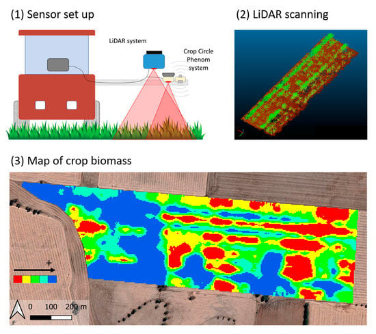
:Crop biomass is an important attribute to consider in relation to site-specific nitrogen (N) management as critical N levels in plants vary depending on crop biomass. Whilst LiDAR technology has been used extensively in small plot-based phenomics studies, large-scale crop scanning has not yet been reported for cereal crops. A LiDAR sensing system was implemented to map a commercial 64-ha wheat paddock to assess the spatial variability of crop biomass. A proximal active reflectance sensor providing spectral indices and estimates of crop height was used as a comparison for the LiDAR system. Plant samples were collected at targeted locations across the field for the assessment of relationships between sensed and measured crop parameters. The correlation between crop biomass and LiDAR-derived crop height was 0.79, which is similar to results reported for plot scanning studies and greatly superior to results obtained for the spectral sensor tested. The LiDAR mapping showed significant crop biomass variability across the field, with estimated values ranging between 460 and 1900 kg ha−1. The results are encouraging for the use of LiDAR technology for large-scale operations to support site-specific management. To promote such an approach, we encourage the development of an automated, on-the-go data processing capability and dedicated commercial LiDAR systems for field operation.
1. Introduction
Crop dry biomass is an important parameter for nutrient management. According to nitrogen (N) dilution theory, the N level in plants varies depending on crop biomass [1,2]; that is, the N concentration—and the minimum N concentration associated with maximum plant growth (the critical N level)—tends to decrease with increasing biomass. In summary, if biomass information is accessible, growers can set a target plant N concentration for mid-season fertilisation using pre-established N dilution models [3]. However, because of the necessity for destructive sampling and laboratory analysis, the high cost and labour required for the assessment of this crop parameter at the field level are impediments for the use of biomass information as a guide for N fertilisation underpinned by an N dilution framework [4]. Thus, alternative approaches for N management are often preferred by farmers, such as the use of empirical N response functions, or estimation of N demand (the final N uptake prediction) and supply for recommendations based on mass balance. However, sensor-based solutions underpinned by these N strategies lack robust evidence supporting their economic benefit [5].
The normalized difference vegetation index (NDVI) based on red and near-infrared reflectance is one of the most common remote and proximal sensing indices used in agriculture and is often regarded as a surrogate for crop cover [6]. Early descriptions of NDVI characterise it as mostly sensitive to ‘green biomass’ [7], but its value is normally affected by both plant N concentration, as the red light is absorbed by chlorophyll, and by the amount of vegetation that reflects near infra-red radiation. This mixed influence may hinder the effective and independent estimate of crop biomass, or plant N status, as required for the assessment of crop nutritional status based on critical N levels. The NDRE (normalized difference red-edge index) which uses the red-edge waveband (~730 nm) instead of the red (~670 nm), is similarly affected by these factors, although it is usually regarded as more sensitive to N concentration than NDVI [8,9]. A recent enhancement to one of the most common ground-based crop sensing technologies, the Crop Circle sensor (Holland Scientific, Lincoln, NE, USA) which formerly provided measurements of spectral indices only [5,10], now also allows estimates of crop height to be made, along with multiple ambient and canopy parameters for crop phenotyping (https://hollandscientific.com/, accessed on 10 August 2021), which may contribute to crop biomass assessment. However, to our knowledge, there has been no independent investigation of the performance of this particular crop sensor.
A large body of recent research (see below) suggests that light detection and ranging (LiDAR) technology is a potential solution for plant biomass assessment at the field level. Ground based LiDAR sensors have been used to assess the physical characteristics of targets for a range of industries and applications. This technology is based on the emission of a laser beam in several directions to compute a ‘point cloud’ which digitally represents the surroundings of the sensor. Since the early 2000s, and arguably inspired by developments in the forestry industry, researchers have extensively investigated this technology for tree crops (see Colaço et al., [11] for a review) to enable site-specific (or tree-specific) management [12,13,14] and crop phenotyping [15]. Its use for cereal crops invariably faces an additional challenge relating to the relatively small size of a target such as a wheat plant, especially in early growth stages. Such challenges may lead to a need for higher sensor performance (e.g., higher scanning frequency) and careful setup with mobile platforms. Thus, research on the use of LiDAR for cereal crops has, in the main, been focused on the scanning of small plots by dedicated mobile platforms with acquisition designed for high-throughput phenotyping of breeding plots (see reviews of Dworak et al. [16], White et al. [17] and Lin [18] and more recent examples by Yuan et al. [19], Jimenez-Berni et al. [20], Walter et al. [21] and Deery et al. [22]). Examples of such dedicated self-propelled scanning platforms are the Phenomobile [23] and the Field Scanalyzer [24] which enable detailed crop scanning at low travel speeds and with stable sensor positioning and orientation. There has also been scanning of field plots based on static (tripod-mounted) LiDAR systems [25]; these are also unsuitable for large scale operations. Overall, farm scale applications focused on decision making in the scope of digital or precision agriculture are still lacking [11]. The work of Elhert et al. [26], following from earlier developments of a crop density sensor [27], and Eitel et al. [28] are examples of studies aimed at developing LiDAR technology for wheat from the perspective of N decision making (even though N recommendations were not derived from the sensors in these examples), but field tests were still confined to small field plots. Shendryk et al. [29] have recently investigated drone-based LiDAR for N management in sugarcane, with measurements also taken from plot trials. Another drone-based LiDAR application was reported by Bates et al. [30] on a 10 ha wheat field in Germany. However, the main issue with the use of drones, or other unmanned aerial vehicles, has been their low operational efficiency in large scale farming systems in which scanning of hundreds of ha must be completed under constrained timeframes. One study that deployed a LiDAR sensor for large scale application is reported by Long and McCallum [31], but their goal was to assess wheat straw biomass at harvest by attaching the LiDAR sensor to a harvester; straw yield maps were generated for two fields of 12 and 20 ha each. The study of Eitel et al. [32] generated a crop biomass map for a 36-ha wheat field. However, in this case, the LiDAR sensor was not used to map the field but to generate a calibration to convert a satellite image into a biomass map for the field.
To the knowledge of the authors, there has been no report of a broadacre application of LiDAR technology aimed at mapping cereal crop physical attributes for precision agriculture purposes (the term ‘broadacre’ refers to large scale commercial farming which, for Australian wheat growers, typically infers a farm size of the order of 2500 ha and fields > 50 ha). Limitations to broadacre applications are normally related to operational challenges associated with upscaling. For example, the more difficult environment for scanning which might include a rougher soil surface, and the need to attach the sensing system to a vehicle adapted to large scale field operations, such as a tractor or an all-terrain vehicle, may increase sensor vibration and rotation (roll, pitch and yaw movements). Thus, there is likely a need for appropriate instrumentation and acquisition set up (including software) to make the system suited for a large scale field operation; a large amount of data and associated data processing, resulting from field scanning [13] presents an additional challenge.
In contrast to previous research on the application of LiDAR technology for small plot applications, this work sought to implement and test a mobile terrestrial laser scanner for biomass estimation on a large wheat field to promote site-specific, sensor-based N management. More specifically, we tested a mobile laser scanning system for large scale mapping of crop biomass against a more common and commercially available ground-based crop sensing technology for broadacre application, in this case, an active optical reflectance sensor. In a follow-up paper, we will propose a multi-sensor N decision framework underpinned by consideration of N dilution and N critical levels and based on LiDAR and reflectance sensors for biomass and N concentration assessment.
2. Materials and Methods
2.1. Field Experimental Design
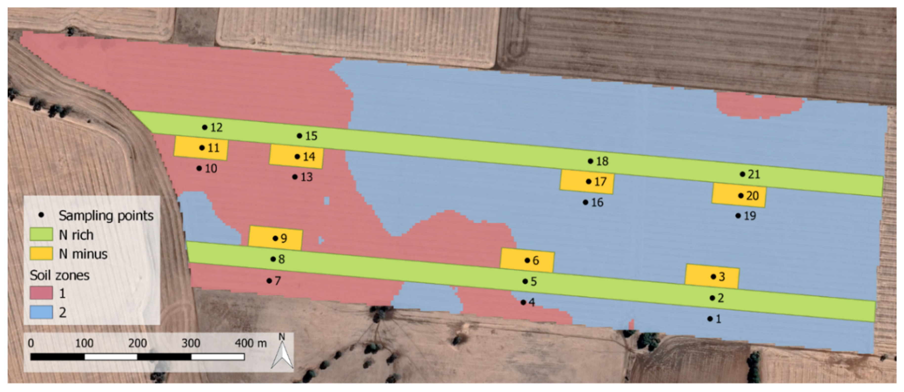
A 64-ha commercial wheat field cultivated under a no-tillage system near Tarlee in South Australia was used for this study during the 2019 season. An on-farm, spatially distributed experimental design [33] was implemented to use the range of variability in the field for the assessment of relationships between the various measured and sensed crop parameters. The design featured areas with different N rates (N ‘rich’ and N ‘minus’ strips) to maximize crop variability and sampling points scattered across the field area (Figure 1). N ‘rich’ strips were 39 m wide (equivalent to the width covered by a single pass of the fertiliser equipment) and approximately 1300 m long and crossed different soil zones previously identified in the field. These zones were defined based on clustering of soil information layers derived from electromagnetic induction (EM38 sensor, Geonics, Mississauga, ON, Canada), gamma radiometry (Mole gamma radiometer, The Soil Company, Groningen, The Netherlands) and soil pH (MSP sensor, Veris Technologies, Salina, KS, USA) surveys. There were seven shorter N ‘minus’ strips of 39 m by 100 m which were spread across the soil zones—three in each zone and one in an intermediate area. Sampling points were positioned to cover the range in N treatments and soil zones. At the beginning of crop stem elongation (Z31, [34]) on 1 August 2019, the crop was scanned with a mobile, ground-based, multi-sensor platform (see below) and plant samples were collected at the 21 sampling points. Plant samples consisted of two crop rows (spaced by 0.3 m) of 1 m length measured for above-ground dry biomass, N concentration and crop height; the average of five manual measurements of crop height was taken with the measurement aimed at the top of the canopy which was visually identified. By the time of crop scanning and sample collection, total applied N rates in the ‘minus’, ‘normal field’ and ‘rich’ treatments were 11, 57 and 141 kg N ha−1 (Table 1); fertiliser was applied with field machinery equipped with RTK-GNSS (Real Time Kinematics—Global Navigation Satellite System) guidance and variable rate technology.
2.2. Sensor Setup
The sensing platform consisted of a LiDAR and a multiparameter canopy sensor system (Crop Circle Phenom, Holland Scientific, Lincoln, NE, USA). The LiDAR system comprised a laser scanner (LMS-400, SICK AG, Waldkirch, Germany), an inertial measurement unit (IMU; Spatial, Advanced Navigation, Sydney, Australia) and a dual-antenna differential GNSS (BD992, Trimble, Sunnyvale, CA, USA). The LiDAR sensor operates at the red wavelength (650 nm) and uses the ‘phase-shift’ principle to calculate the distance between the sensor and target—the returned light has a difference in phase to the emitted light, which is proportional to the travelled distance. The distance is recorded for each 0.1° angular step along a 70° field of view, with complete rotation at 270 Hz. The system was activated and controlled with a developed Robot Operating System (ROS; Stanford University [35]). The Crop Circle Phenom system comprised a multispectral active reflectance sensor (Crop Circle ACS-435) operating at the red (670 nm), red-edge (730 nm) and near-infrared (780 nm) wavelengths and a multi-parameter sensor (Crop Circle DAS43X) assessing ambient and canopy parameters at 1 Hz of measurement frequency. The selected variables from the Crop Circle Phenom system relevant to this study were NDVI, NDRE and crop height from the ACS-435 sensor and photosynthetic active radiation (PAR; given as the ratio between reflected and incident radiation) from the DAS43X sensor. According to the sensor specifications, crop height estimation is derived from a built-in calibration based on the inverse-square law response of the irradiance measurement of the sensor. The response of the irradiance measurement to sensor-target distance is transformed into a linear relationship (see Holland et al. [36] for detail), with crop height given as the sensor mounting height (above ground) minus the estimated target distance. A separate differential GNSS was used for the Crop Circle system (S321, Hemisphere, Scottsdale, AZ, USA).
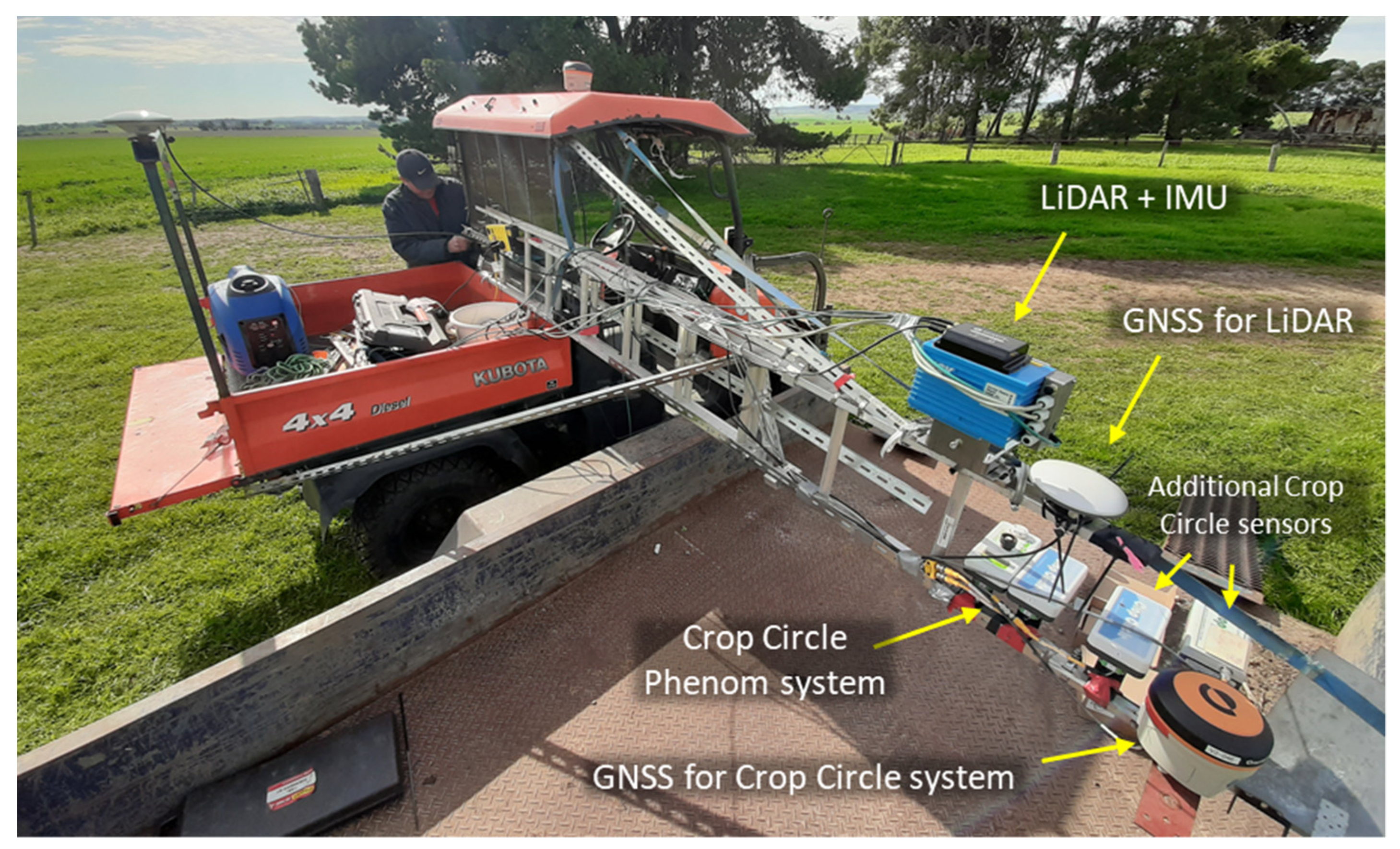
The sensors were mounted onto a platform attached to the side of an all-terrain vehicle with the LiDAR system at 1.3 m above the ground for a vertical scanning (nadir) of the crop (Figure 2 and Figure 3). The Crop Circle sensors were attached alongside the LiDAR system at 1 m above the ground. The sensors were arranged so that they did not block each other’s field of view (by facing opposite directions) whilst having an overlapping scanned area on the ground. For field scanning, the system was operated along 11 transects of the field (tramlines spaced by 39 m) at a travel speed of 2.2 m s−1.
2.3. Data Processing
The data from the LiDAR and IMU sensors were processed using Robot Operating System middleware to generate a 3D point cloud which was georeferenced based on the GNSS track data. The point cloud output represented all laser hits on the crop canopy and on the ground. For processing the point cloud, the data collected along the 11 transects were split into batches of approximately 15 million points and processed in the following steps using Cloud Compare software (version 2.10.2, Cloud Compare [GPL software] [37]): (i) load the point cloud data for visual inspection; (ii) remove isolated points using the ‘Statistical Outlier Removal’ tool using default parameters (number of points for mean distance estimation = 6; standard deviation multiplier = 1); (iii) classification of points into ground (soil and straw left from the previous crop) and above-ground (plant canopy) points using the ‘Cloth Simulation Filter’ (CSF) plugin tool [38] with parameters set as Scene = flat, cloth resolution = 0.1, max iterations = 1000 and classification threshold = 0.1; (iv) apply ‘Rasterize’ tool to compute average point height and total point count rasters of 0.25 m resolution for each of the ‘ground’ and ‘above ground’ point clouds. The two rasters were then imported into QGIS software (version 3.10, QGIS Development Team [39]) and the ‘Raster Calculator’ tool was used for the extraction of two crop parameters: crop height, given as the difference in height between ‘ground’ and ‘above ground’ points, and canopy cover, given as the ratio between the ‘above ground’ and ‘total’ point count. Note that for the height calculation, the average height of ‘plant’ points was used instead of the top of the canopy (i.e., the maximum point height). Because of the fewer points representing the top of the canopy—especially after outlier elimination—this strategy was considered to produce a more robust and representative assessment of the crop.
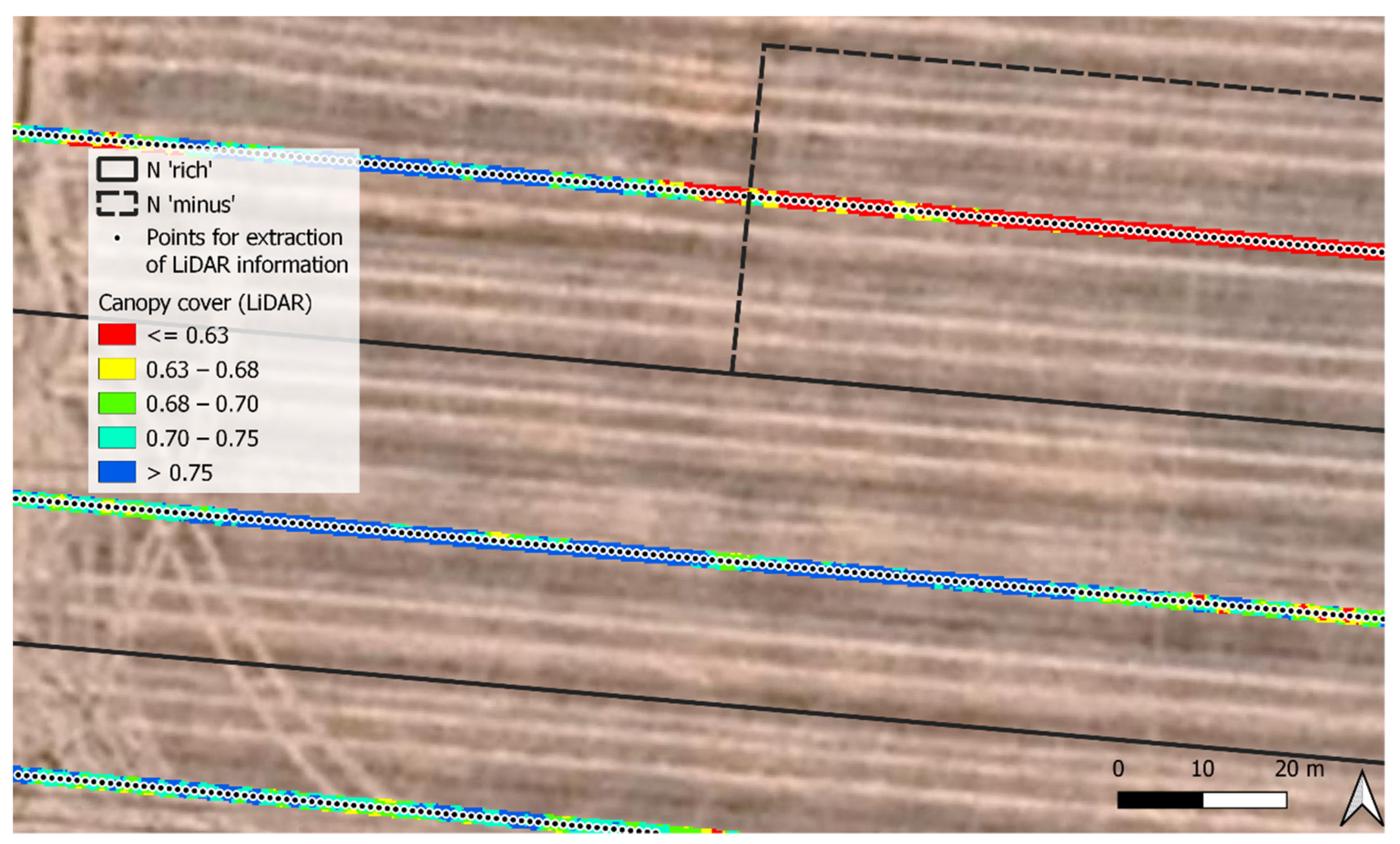
To produce interpolated maps of crop height and canopy cover for the entire area, a sequence of lined points spaced 1 m apart, totalling approximately 225 points ha−1, was created along the length of each transect (Figure 4). The raster information (crop height and canopy cover) was extracted for each point using the average of a 3 × 3-pixel window. The point data were then interpolated using local block kriging into a 5 m pixel grid with block size set to 30 m. These processing steps were conducted using the PAT plugin tool for QGIS [40]; the Vesper software [41], activated through PAT, was used for kriging interpolation. The Crop Circle data (NDVI, NDRE, crop height and PAR) was processed for outlier elimination and interpolated into the same pixel grid using local block kriging (block size was also 30 m). Although maps were generated using local block kriging (i.e., with a local variogram), the global variograms for each variable using Vesper software were also analysed for a better understanding of the spatial structure of the data. The final database from field collection consisted of interpolated maps and a point dataset with sensed data and measured dry biomass (kg ha−1), N concentration (%) and crop height (m). Relationships between variables were assessed using linear regression.
3. Results
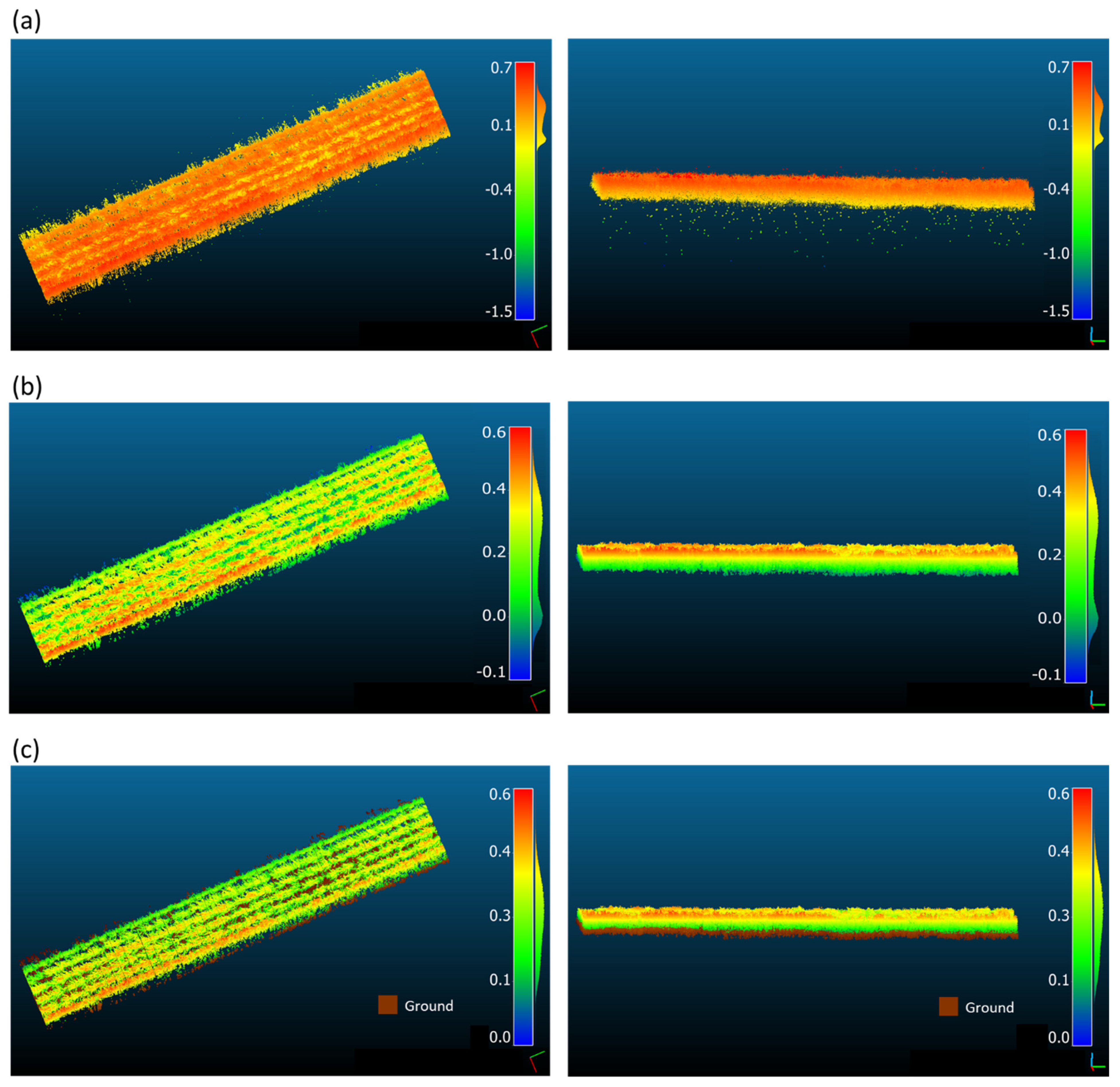
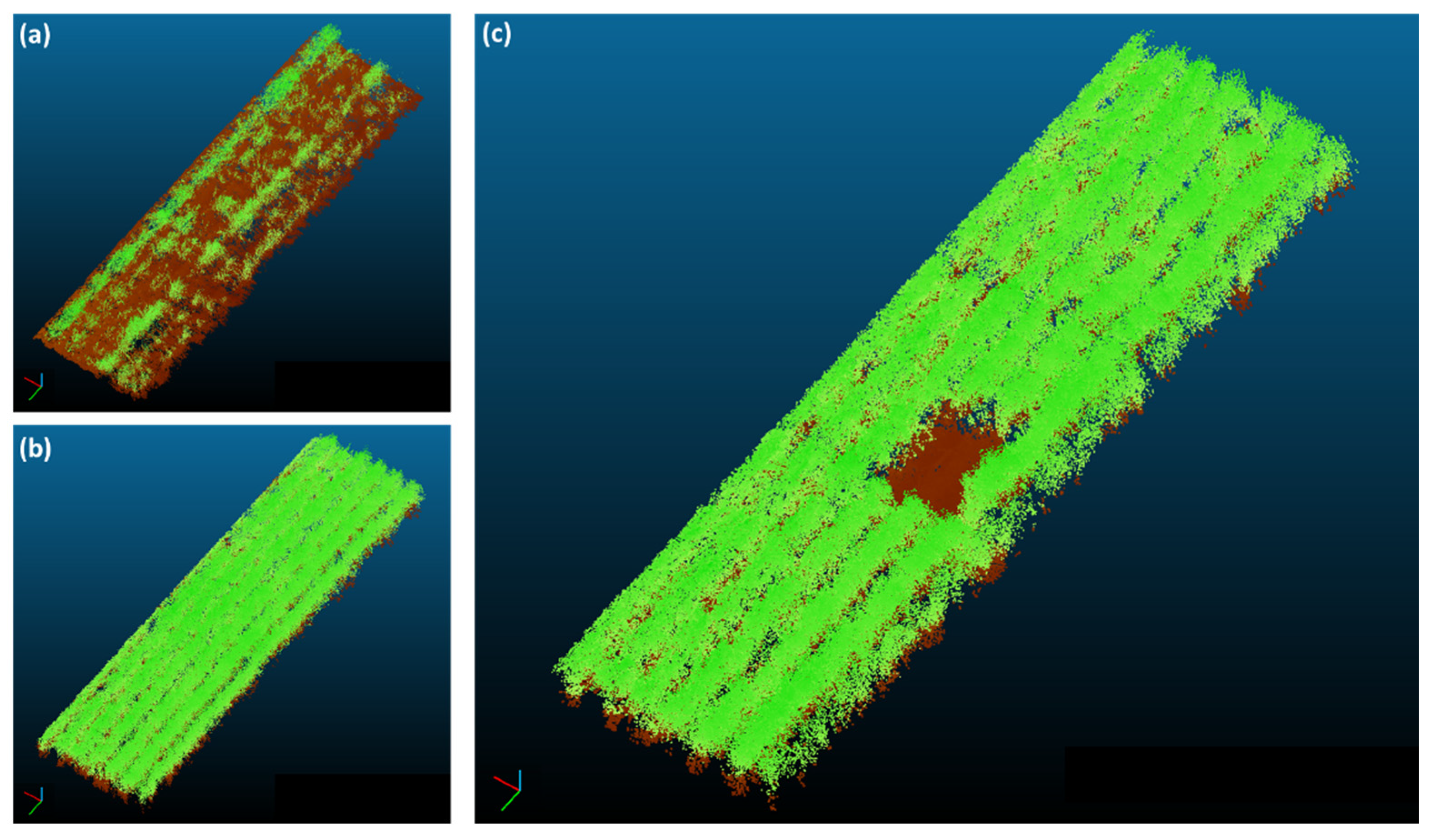
The LiDAR crop scanning resulted in approximately 884 million points across the 64-ha paddock. With a total scanned area of approximately 3 ha (4.5% of the total area) and an average point elimination of 7% of outliers, the ground point density was approximately 28,000 points m−2. Figure 5 illustrates the data processing steps from the raw data to the filtered and classified point cloud into ground and above ground points. Based on a visual inspection, both the filtering and classification steps seem to have worked satisfactorily. In Figure 5, the top figures show the raw point cloud with outlier points mostly in the bottom part of the cloud which were eliminated after filtering (middle figure); note that the point height ranged between −1.5 and 0.7 m before outlier elimination, and after filtering, points were concentrated mostly around the 0 and 0.3 m height levels. Figure 5 also shows that points closer to the ground level were classified as ‘ground’ points (bottom figure). Overall, the final processed point cloud was judged to have represented the crop in sufficient detail to distinguish different levels of crop cover and general development (Figure 6). The actual validation of the digital information generated from the LiDAR is provided below based on the ground truth plant measurement.
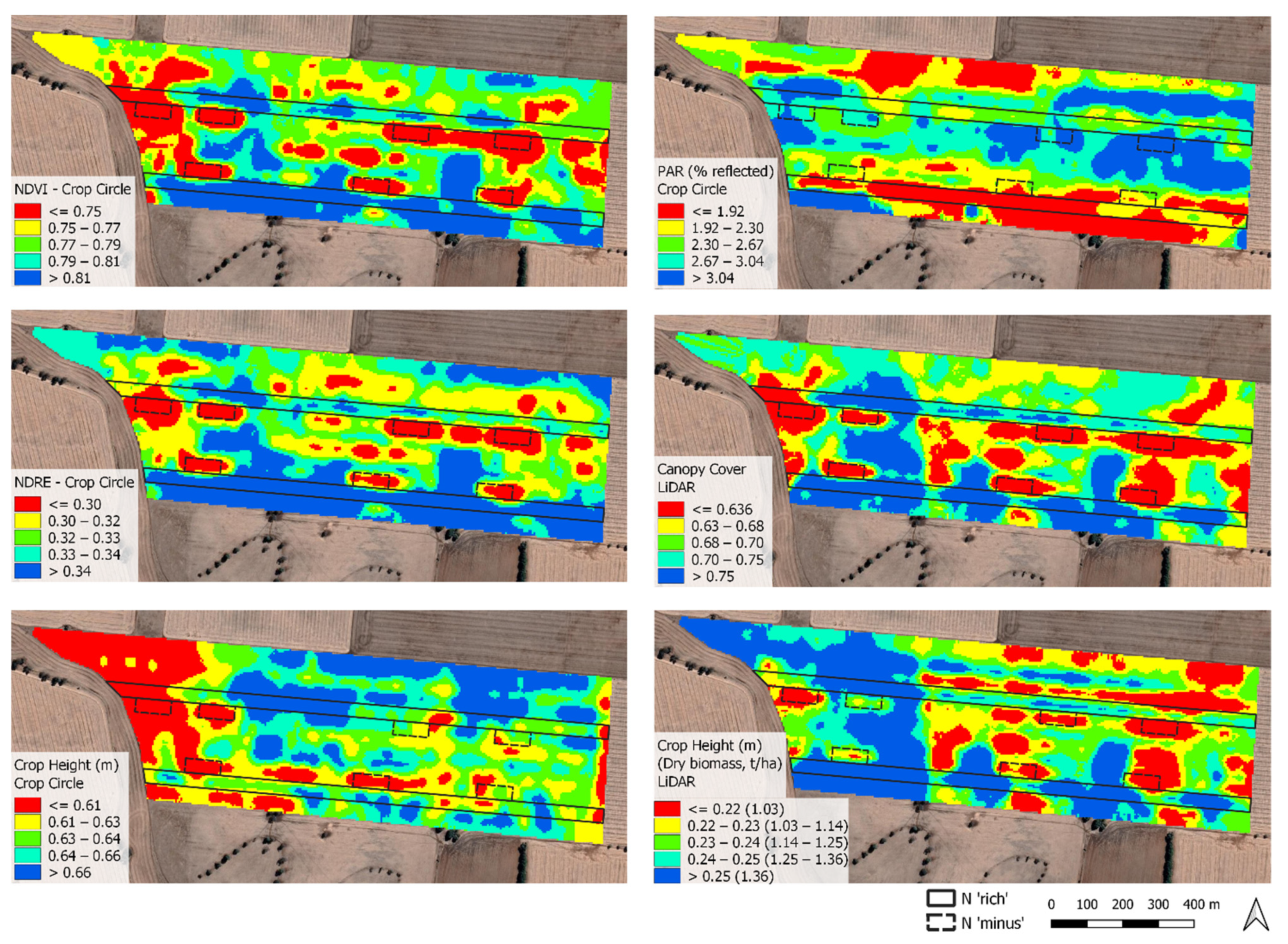
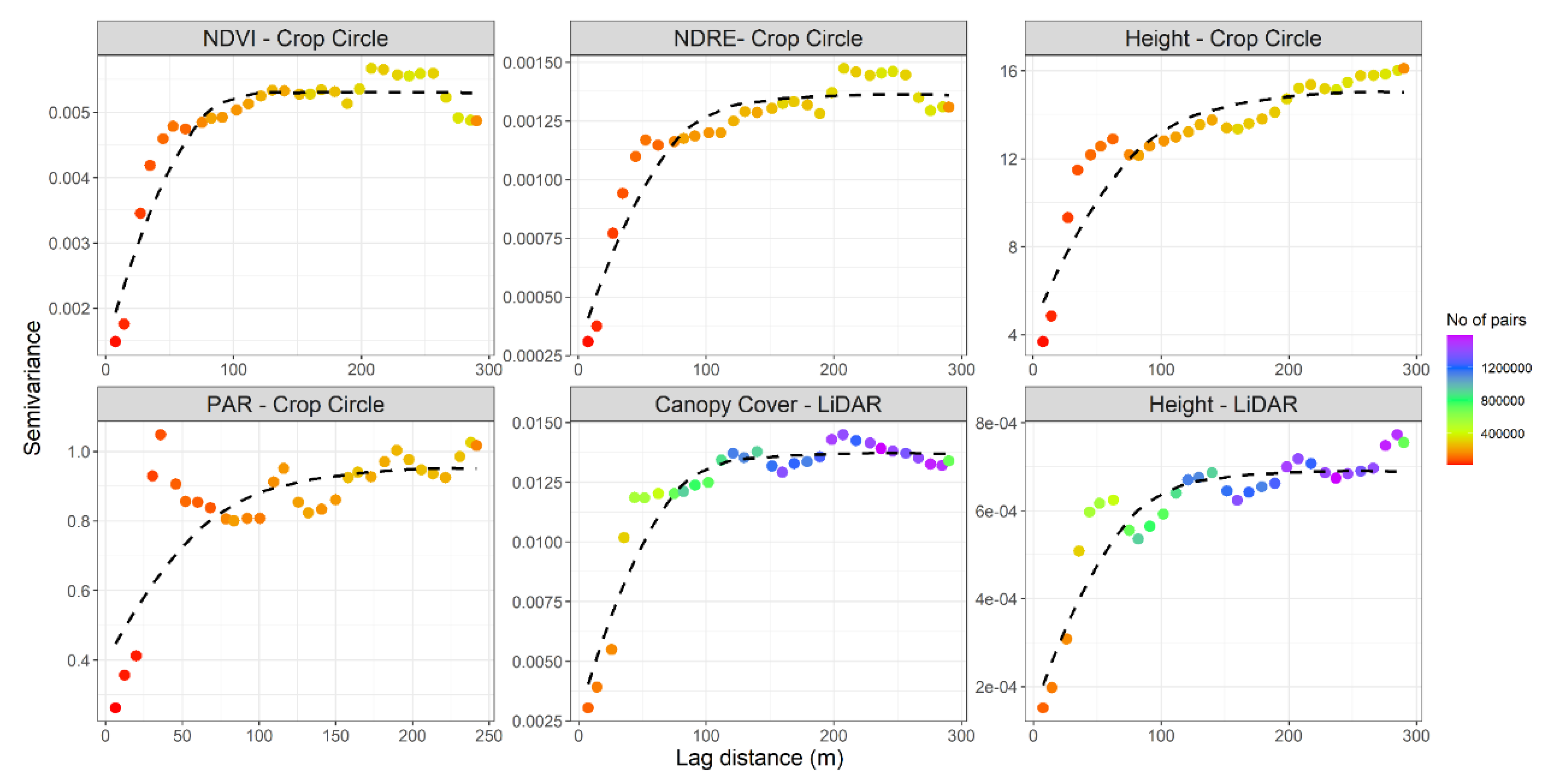
Maps derived from the Crop Circle and LiDAR systems are shown in Figure 7. The global variogram for each sensor variable is presented in Figure 8 for a better understanding of the spatial structure of the data. The variogram analysis shows similar spatial structures across the different variables; note below that most sensed variables were correlated with each other, to varying degrees (Table 2). All variograms had low ‘nugget’ variance with the sill variance being reached between 100 and 150 m; that is, a range of spatial dependence of 100–150 m. Similar to the Crop Circle data, LiDAR-derived parameters showed strong spatial dependence, with resulting maps indicating structured spatial patterns across the field. This indicates that the implemented LiDAR system, from data acquisition through to processing (including the virtual points approach to spatially distribute the LiDAR information; shown in Figure 4), provided adequate data for mapping crop variability and thus, potentially supporting site-specific management. Overall, LiDAR maps had similar general spatial patterns to the NDVI and NDRE maps, with the effect of the N strips being easily identified through these maps. The influence of the different soil types (Figure 1) was somewhat evident on the NDVI, NDRE, LiDAR crop height and LiDAR canopy cover maps; i.e., soil zone 1 generally provided more suitable conditions for crop growth than soil zone 2. Using a calibration between LiDAR crop height and crop biomass (see below), the LiDAR mapping shows an estimated variability in crop biomass between 460 and almost 1900 kg ha−1 across the field, which is critically important for site-specific nutrient management. Crop height and PAR derived from the Crop Circle sensing system had different spatial patterns with N strips less evident through these maps.
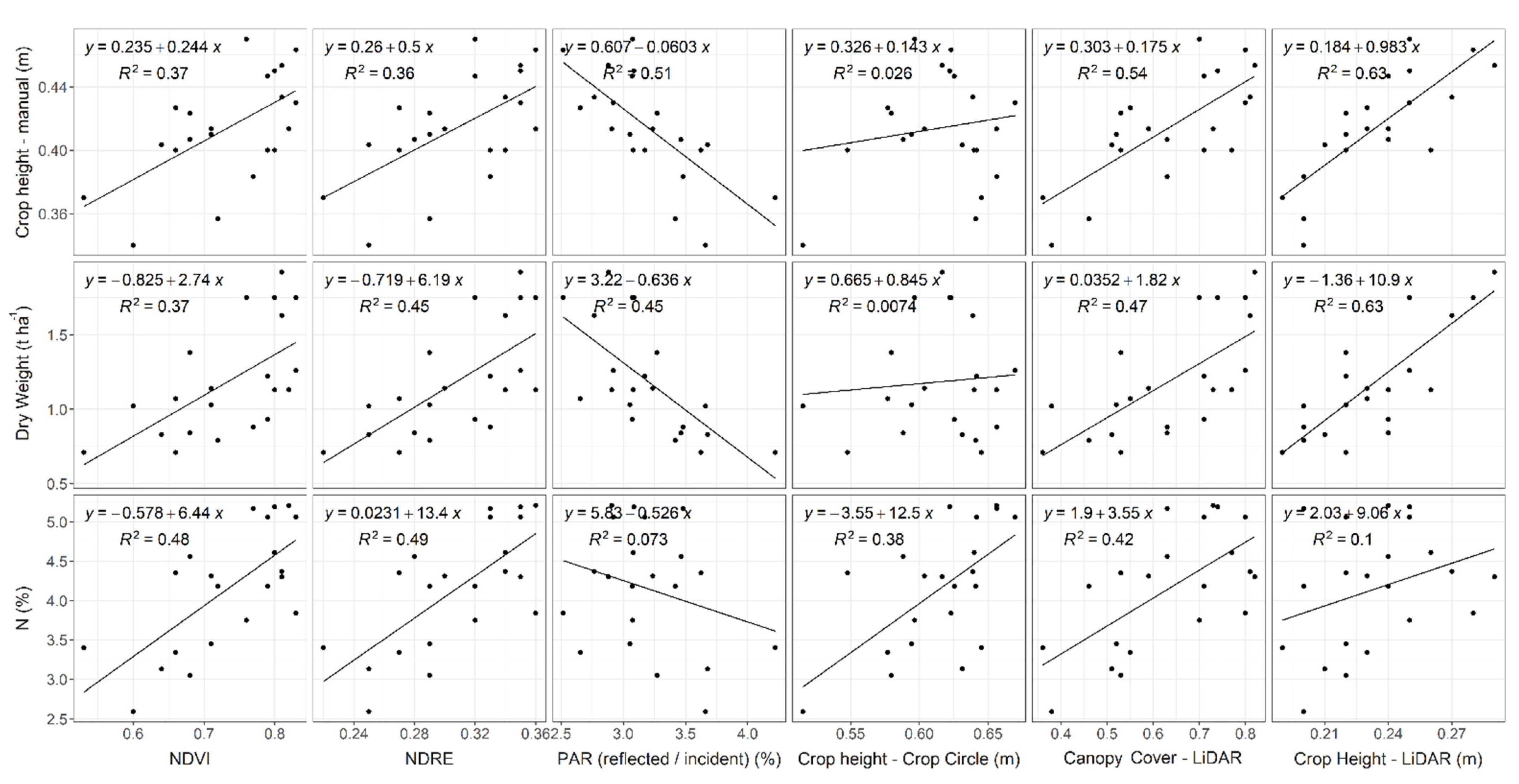
The relationships between sensed and measured crop parameters are shown in Figure 9 and Table 2. Overall, the LiDAR-derived crop height outperformed estimations of biomass from the Crop Circle sensor. As expected, NDVI and NDRE were influenced by both plant N concentration and dry biomass. Of interest, these indices were well correlated with total N uptake calculated as total N per unit area (crop dry weight multiplied by N%), with a coefficient of determination over 0.7 (data not shown). However, as noted above, N management practices underpinned by critical N levels depend on the information of biomass and N concentration independently. LiDAR-derived crop height was well correlated with crop biomass (R2 = 0.63, r = 0.79, root mean squared error (RMSE) = 218 kg ha−1), with no relationship with plant N concentration, which indicated that LiDAR-derived height is a more appropriate surrogate to crop biomass then spectral indices. LiDAR height was also reasonably correlated with manual measures of height, although it should be noted that the LiDAR sensor estimated the average point height of the canopy whereas the manual measures aimed to assess the height of the top of the canopy. LiDAR-derived canopy cover had a similar behaviour to NDVI and NDRE with a moderate relationship with both N concentration and crop biomass; canopy cover was highly correlated with NDRE and NDVI (see also maps in Figure 7).
Crop height derived from the Crop Circle sensor had the weakest relationships with all other sensed and measured variables, including manual crop height; note that crop height estimates were normally greater than manual measurements; also the Crop Circle height map showed little resemblance with all other maps. These initial results are not encouraging for the application of this estimate for either crop phenotyping or nutrient management, but further investigations are encouraged. Variation in the sensor mounting height may have affected the sensor performance as the crop height estimate relies on a constant sensor height to the ground. In addition, the distance measurement provided by the Crop Circle sensor assumes a uniform target reflectance within the sensor field of view (Holland et al. [36]). This constraint likely introduces error into the measured height values when scanning a crop with a heterogeneous canopy. However, the results from the variogram analysis (low nugget) do not suggest there was significant noise in the data. The LiDAR system is not affected by this issue as height is computed based on the difference between canopy and ground height level, with the sensor rotation also being corrected based on the IMU readings. PAR from the Crop Circle Phenom sensor had only a moderate relationship with crop manual height and biomass with little relationship to the N concentration.
4. Discussion
To our knowledge, this is the first report on the use of a LiDAR scanning system for commercial field-scale mapping of a cereal crop; as indicated, previous LiDAR research has overwhelmingly focused on plot scanning, with large-scale applications mostly investigated for horticultural crops. Moreover, most studies on cereal crops have implemented systems based on dedicated phenomics platforms, drones or static tripod-mounted sensors, which may be unsuitable for large scale applications. Contrary to these approaches, the mobile terrestrial system tested in this study can be easily implemented using field machinery (such as a tractor) so that the scanning can occur while other operations take place. Overall, the results in this study indicate the potential for the use of this technology for crop biomass mapping in the context of precision agriculture and site-specific nutrient management. Biomass information can be combined with N% estimates from spectral indices (for example the Canopy Chlorophyll Content Index; CCCI [3]) to allow variable-rate N application mid-season using a ‘N sufficiency’ approach based on N dilution and critical N levels. That is, the N recommendation would aim at a target plant N concentration associated with a target crop biomass (this decision framework will be proposed and demonstrated in the following paper).
The scanning system which included custom sensor supports and data acquisition software performed well under field conditions. Colaço et al. [13] reported the failure of a SICK LMS 200 LiDAR sensor due to high light exposure into the sensor detectors during the vertical scanning of orange trees on a large-scale operation. This was not an issue for the present study as the sensor was positioned for a nadir scanning meaning that sunlight did not hit the sensor detectors directly. However, despite the good results from an operational perspective, the difficulty of handling the large dataset derived from field scanning and the laborious manual steps involved in the processing of the LiDAR point cloud can be regarded as significant impediments for the application of this technology. In particular, the data had to be processed in batches, rather than for the whole field, so that a standard desk computer could cope with both data processing and display. Ideally, an alternative, automated, on-the-go data processing approach is needed for LiDAR to be a viable input to precision agriculture applications such as fertiliser management. In this case, given that the focus was on crop height, it is suggested that this may be possible; for example, by processing small batches of data (e.g., each scan or a few consecutive scans) on the go (i.e., while the data is being collected) and storing only the output parameter of interest.
The correlation between crop biomass and LiDAR-derived crop height obtained in this study (r = 0.79) is generally comparable with results obtained from plot-based phenomics studies, and in some cases even slightly higher. For example, the studies of Walter et al. [21] and Deery et al. [22] show variable results across experiments and sampling dates but the best correlations reported for a Z31 growth stage were around 0.72 for both studies. In this study, the biomass estimate error (RMSE) from the LiDAR canopy height was 218 kg ha−1. If the N dilution effect is ignored and a constant N concentration of 4% is assumed, a biomass error of 218 kg ha−1 equates to approximately 8 kg N ha−1 of N uptake. We believe this to be a reasonable error in the context of the N application. Yet, further investigation around the minimum accuracy required for biomass estimation in the context of N management is encouraged.
Whilst this initial work shows promising results for crop mapping using a LiDAR sensor, further research must continue to develop and evaluate biomass estimations for the successful implementation of this technology at the farm level. There are several questions worthy of further investigation, as follows.
First, LiDAR-derived parameters other than crop height could potentially be used for biomass estimation—either as stand-alone variables or in combination with others. Although crop height is amongst the most common parameters for biomass estimation [17], other parameters extracted from the point cloud should be evaluated. For example, volume parameters based on ‘voxels’—where each point is attributed with a small cubic volume [20] could be explored. Likewise, ‘hull’-based approaches—where outer points are connected to form an enclosed virtual object representing the plant canopy [13] may be useful. Variations on these ideas, such as prism or column voxelization [21,42] could be explored. Walter et al. [21] reported a correlation of 0.86 between ‘LiDAR Projected Volume’ and crop biomass for a Z31 scanning in one of their experiments. However, whilst volume-based indicators may result in better correlations with crop biomass than crop height, it is worth noting that both parameters investigated in the present study (crop height and canopy cover) were chosen for their easy processing across a large dataset and robustness for field conditions. Crop height, as calculated in this study (average height of canopy points minus the average height of ground points) can be regarded, by definition, as relatively resilient to changes in point cloud density, which can be caused by variations in travel speed, for example. In summary, all that is needed for the extraction of this attribute is enough points to represent the average height of the canopy and ground levels; the other volume-based attributes mentioned above are, by definition, directly affected by the point cloud density. This leads to a second question regarding the minimum point cloud density needed for assessing crop height, which might possibly be much less than what was used in this study. A similar suggestion was raised by Hammerle and Hofle [43]. The use of a lower-density point cloud—the opposite of what is normally aimed for in plot phenotyping—should greatly facilitate data processing, also likely allowing a larger area of the crop to be scanned, both of which should contribute to upscaling of the technology for field-scale applications. It is also true that increasing the resolution of field information indiscriminately is not useful for crop management given the limited resolution of field machinery.
Third, the question of scanning configuration and orientation needs examination. For example, some studies used the LiDAR sensor on an angle (not in a nadir position as in this study) which might facilitate the laser penetration into the canopy and onto the ground depending on the plant architecture, row spacing and growth stage [44,45]. All these and other questions could be addressed virtually using computer models [46] and of course, subsequently tested under field conditions.
Finally, it is also worth noting the lack of commercial products suited for the specific conditions of broadacre agricultural field scanning. In contrast to the Crop Circle sensor and other similar sensors, which were developed specifically for the kind of application described here, the LiDAR system had to be customized. Critically, this customization included in-house software development for operating the system and collecting data. Eitel et al. [28] made a similar comment about the need for easy to use commercial products that have been specifically designed for agricultural applications. The fact that LiDAR systems are generally not supplied with simple data acquisition and processing software impedes their rapid adoption in agriculture. Investigation of alternative technologies such as machine vision with RGB imaging for large scale biomass mapping is also encouraged. Of course, such solutions would also need to be implemented in simple and dedicated products to promote their adoption and commercial use.
5. Conclusions
A ground-based mobile LiDAR system was successfully deployed for mapping crop biomass in a commercial broadacre wheat field in South Australia. This was an advance on previous research which has overwhelmingly been confined, in cereal crops, to phenomics applications in small field plots. The crop height map derived here enabled assessment of biomass variability across the field as an input to variable-rate N application underpinned by a N dilution framework—as critical N levels are dependent on crop biomass.
The implemented sensing platform including a LiDAR and inertial measurement unit, along with the proposed data processing steps allowed estimates of crop biomass based on LiDAR-derived crop height to be similar to those obtained in more controlled studies based on field plots and dedicated phenomics sensing platforms. This system greatly outperformed spectral indices and a crop height estimate provided by a commercial active optical multispectral sensor.
To continue to promote LiDAR technology at the field level for farm decision making, we encourage more studies on the continuous development and evaluation of sensor estimates of crop biomass across different field scenarios, the development of automated and on-the-go data processing and, finally, the development of commercial LiDAR systems dedicated for agricultural field operation.
Author Contributions
Conceptualization, all authors; methodology, all authors; formal analysis, A.F.C. and M.S.; writing—original draft preparation, A.F.C.; writing—review and editing, all authors; supervision, R.G.V.B.; project administration, R.G.V.B.; funding acquisition, R.G.V.B. All authors have read and agreed to the published version of the manuscript.
Funding
This work was jointly funded by CSIRO and the Grains Research and Development Corporation (GRDC) as a part of the ‘Future Farm’ project (GRDC Project 9176493) in which the University of Sydney, University of Queensland, Queensland University of Technology and Agriculture Victoria are also collaborators.
Acknowledgments
We are most grateful to Damian Mowat and Michael Pritchard (CSIRO/High Resolution Plant Phenomics Facility) for their excellent technical assistance and input, and to Mark Branson for allowing us to conduct trials on his farm. We are also grateful to David Deery and Everard Edwards (CSIRO) for their helpful comments on an earlier draft of the manuscript.
Conflicts of Interest
The authors declare no conflict of interest. The funders had no role in the design of the study; in the collection, analyses, or interpretation of data; in the writing of the manuscript, or in the decision to publish the results.
References
- Lemaire, G.; Gastal, F. N Uptake and Distribution in Plant Canopies. In Diagnostics of the Nitrogen Status in Crops; Lemaire, G., Ed.; Springer: Berlin/Heidelberg, Germany, 1997; pp. 3–43. [Google Scholar]
- Lemaire, G.; Sinclair, T.; Sadras, V.; Bélanger, G. Allometric approach to crop nutrition and implications for crop diagnosis and phenotyping. A review. Agron. Sustain. Dev. 2019, 39, 1–17. [Google Scholar]
- Fitzgerald, G.; Rodriguez, D.; O’Leary, G. Measuring and predicting canopy nitrogen nutrition in wheat using a spectral index—The canopy chlorophyll content index (CCCI). Field Crop. Res. 2010, 116, 318–324. [Google Scholar] [CrossRef]
- Lemaire, G.; Jeuffroy, M.H.; Gastal, F. Diagnosis tool for plant and crop N status in vegetative stage. Theory and practices for crop N management. Eur. J. Agron. 2008, 28, 614–624. [Google Scholar] [CrossRef]
- Colaço, A.F.; Bramley, R.G.V. Do crop sensors promote improved nitrogen management in grain crops? Field Crop. Res. 2018, 218, 126–140. [Google Scholar] [CrossRef]
- Fitzgerald, G.J. Characterizing vegetation indices derived from active and passive sensors. Int. J. Remote Sens. 2010, 31, 4335–4348. [Google Scholar] [CrossRef]
- Rouse, J.W.; Hass, R.H.; Schell, J.A.; Deering, D.W. Monitoring Vegetation Systems in the Great Plains with ERTS. In Proceedings of the Third Earth Resources Technology Satellite (ERTS) Symposium, Washington, DC, USA, 10–14 December 1973; Volume 351, p. 309. [Google Scholar]
- Tilling, A.K.; O’Leary, G.J.; Ferwerda, J.G.; Jones, S.D.; Fitzgerald, G.J.; Rodriguez, D.; Belford, R. Remote sensing of nitrogen and water stress in wheat. Field Crop. Res. 2007, 104, 77–85. [Google Scholar] [CrossRef]
- Feng, W.; Zhang, H.-Y.; Zhang, Y.-S.; Qi, S.-L.; Heng, Y.-R.; Guo, B.-B.; Ma, D.-Y.; Guo, T.-C. Remote detection of canopy leaf nitrogen concentration in winter wheat by using water resistance vegetation indices from in-situ hyperspectral data. Field Crop. Res. 2016, 198, 238–246. [Google Scholar] [CrossRef]
- Franzen, D.W.; Kitchen, N.R.; Holland, K.H.; Schepers, J.S.; Raun, W.R. Algorithms for in-season nutrient management in cereals. Agron. J. 2016, 108, 1775. [Google Scholar] [CrossRef] [Green Version]
- Colaço, A.F.; Molin, J.P.; Rosell-Polo, J.R.; Escolà, A. Application of light detection and ranging and ultrasonic sensors to high-throughput phenotyping and precision horticulture: Current status and challenges. Hort. Res. 2018, 5, 35. [Google Scholar] [CrossRef] [Green Version]
- Escolà, A.; Rosell-Polo, J.R.; Planas, S.; Gil, E.; Pomar, J.; Camp, F.; Llorens, J.; Solanelles, F. Variable rate sprayer. Part 1—Orchard prototype: Design, implementation and validation. Comput. Electron. Agric. 2013, 95, 122–135. [Google Scholar] [CrossRef] [Green Version]
- Colaço, A.F.; Trevisan, R.G.; Molin, J.P.; Rosell-Polo, J.R.; Escolà, A. A method to obtain orange crop geometry information using a mobile terrestrial laser scanner and 3d modeling. Remote Sens. 2017, 9, 763. [Google Scholar] [CrossRef] [Green Version]
- Colaço, A.F.; Molin, J.P.; Rosell-Polo, J.R.; Escolà, A. Spatial variability in commercial orange groves. Part 1: Canopy volume and height. Precis. Agric. 2019, 20, 788–804. [Google Scholar] [CrossRef] [Green Version]
- Siebers, M.H.; Edwards, E.J.; Jimenez-Berni, J.A.; Thomas, M.; Salim, M.; Walker, R. Fast phenomics in vineyards: Development of grover, the grapevine rover, and LiDAR for assessing grapevine traits in the field. Sensors 2018, 18, 2924. [Google Scholar] [CrossRef] [PubMed] [Green Version]
- Dworak, V.; Selbeck, J.; Ehlert, D. Ranging sensors for vehicle-based measurement of crop stand and orchard parameters: A review. Trans. ASABE 2011, 54, 1497–1510. [Google Scholar] [CrossRef]
- White, J.W.; Andrade-Sanchez, P.; Gore, M.A.; Bronson, K.F.; Coffelt, T.A.; Conley, M.M.; Feldmann, K.A.; French, A.N.; Heun, J.T.; Hunsaker, D.J.; et al. Field-based phenomics for plant genetics research. Field Crop. Res. 2012, 133, 101–112. [Google Scholar] [CrossRef]
- Lin, Y. LiDAR: An important tool for next-generation phenotyping technology of high potential for plant phenomics? Comput. Electron. Agric. 2015, 119, 61–73. [Google Scholar] [CrossRef]
- Yuan, W.; Li, J.; Bhatta, M.; Shi, Y.; Baenziger, P.S.; Ge, Y. Wheat height estimation using LiDAR in comparison to ultrasonic sensor and UAS. Sensors 2018, 18, 3731. [Google Scholar] [CrossRef] [Green Version]
- Jimenez-Berni, J.A.; Deery, D.M.; Rozas-Larraondo, P.; Condon, A.T.G.; Rebetzke, G.J.; James, R.A.; Bovill, W.D.; Furbank, R.T.; Sirault, X.R.R. High throughput determination of plant height, ground cover, and above-ground biomass in wheat with LiDAR. Front. Plant Sci. 2018, 9, 237. [Google Scholar] [CrossRef] [PubMed] [Green Version]
- Walter, J.D.C.; Edwards, J.; McDonald, G.; Kuchel, H. Estimating biomass and canopy height with LiDAR for field crop breeding. Front. Plant Sci. 2019, 10, 1145. [Google Scholar] [CrossRef]
- Deery, D.M.; Rebetzke, G.J.; Jimenez-Berni, J.A.; Condon, A.G.; Smith, D.J.; Bechaz, K.M.; Bovill, W.D. Ground-based lidar improves phenotypic repeatability of above-ground biomass and crop growth rate in wheat. Plant Phenomics 2020, 2020, 1–11. [Google Scholar] [CrossRef]
- Deery, D.; Jimenez-Berni, J.; Jones, H.; Sirault, X.; Furbank, R. Proximal remote sensing buggies and potential applications for field-based phenotyping. Agronomy 2014, 4, 349–379. [Google Scholar] [CrossRef] [Green Version]
- Virlet, N.; Sabermanesh, K.; Sadeghi-Tehran, P.; Hawkesford, M.J. Field Scanalyzer: An automated robotic field phenotyping platform for detailed crop monitoring. Funct. Plant Biol. 2017, 44, 143. [Google Scholar] [CrossRef] [PubMed] [Green Version]
- Tilly, N.; Hoffmeister, D.; Cao, Q.; Huang, S.; Lenz-Wiedemann, V.; Miao, Y.; Bareth, G. Multitemporal crop surface models: Accurate plant height measurement and biomass estimation with terrestrial laser scanning in paddy rice. J. Appl. Remote Sens. 2014, 8, 083671. [Google Scholar] [CrossRef]
- Ehlert, D.; Adamek, R.; Horn, H.J. Laser rangefinder-based measuring of crop biomass under field conditions. Precis. Agric. 2009, 10, 395–408. [Google Scholar] [CrossRef]
- Ehlert, D.; Schmerler, J.; Voelker, U. Variable rate nitrogen fertilisation of winter wheat based on a crop density sensor. Precis. Agric. 2004, 5, 263–273. [Google Scholar] [CrossRef]
- Eitel, J.U.H.; Magney, T.S.; Vierling, L.A.; Brown, T.T.; Huggins, D.R. LiDAR based biomass and crop nitrogen estimates for rapid, non-destructive assessment of wheat nitrogen status. Field Crop. Res. 2014, 159, 21–32. [Google Scholar] [CrossRef]
- Shendryk, Y.; Sofonia, J.; Garrard, R.; Rist, Y.; Skocaj, D.; Thorburn, P. Fine-scale prediction of biomass and leaf nitrogen content in sugarcane using UAV LiDAR and multispectral imaging. Int. J. Appl. Earth Obs. 2020, 92, 102177. [Google Scholar] [CrossRef]
- Bates, J.S.; Montzka, C.; Schmidt, M.; Jonard, F. Estimating canopy density parameters time-series for winter wheat using UAS mounted lidar. Remote Sens. 2021, 13, 710. [Google Scholar] [CrossRef]
- Long, D.S.; McCallum, J.D. Mapping straw yield using on-combine light detection and ranging (lidar). Int. J. Remote Sens. 2013, 34, 6121–6134. [Google Scholar] [CrossRef]
- Eitel, J.U.H.; Magney, T.S.; Vierling, L.A.; Greaves, H.E.; Zheng, G. An automated method to quantify crop height and calibrate satellite-derived biomass using hypertemporal lidar. Remote Sens. Environ. 2016, 187, 414–422. [Google Scholar] [CrossRef] [Green Version]
- Colaço, A.F.; Bramley, R.G.V. A Spatially Distributed On-Farm Experimental Approach for the Development of a Sensor-Based Nitrogen Decision Model. In Proceedings of the 19th Australian Agronomy Conference, Wagga Wagga, NSW, Australia, 25–29 August 2019; The Australian Society of Agronomy: Toowoomba, Australia; pp. 1–4. [Google Scholar]
- Zadoks, J.C.; Chang, T.T.; Konzak, C.F. A decimal growth code for the growth stages of cereals. Weed Res. 1974, 14, 415–421. [Google Scholar] [CrossRef]
- Stanford Artificial Intelligence Laboratory; Robotic Operating System. 2018. Available online: https://www.ros.org (accessed on 8 October 2020).
- Holland, K.H.; Lamb, D.W.; Schepers, J.S. Radiometry of proximal active optical sensors (AOS) for agricultural sensing. IEEE J. Sel. Top. Appl. Earth Obs. Remote Sens. 2012, 5, 1793–1802. [Google Scholar] [CrossRef]
- Cloud Compare v2.10.2 [GPL Software]. 2020. Available online: http://www.cloudcompare.org (accessed on 8 October 2020).
- Zhang, W.; Qi, J.; Wan, P.; Wang, H.; Xie, D.; Wang, X.; Yan, G. An Easy-to-Use Airborne LiDAR Data Filtering Method Based on Cloth Simulation. Remote Sens. 2016, 8, 501. [Google Scholar] [CrossRef]
- QGIS v3.10—QGIS Development Team. QGIS Geographic Information System. Open Source Geospatial Foundation Project. 2020. Available online: http://www.qgis.org. (accessed on 8 October 2020).
- Ratcliff, C.; Gobbett, D.; Bramley, R.G.V. PAT—Precision Agriculture Tools. v3. CSIRO. Software Collections. 2020. Available online: https://0-doi-org.brum.beds.ac.uk/10.25919/5f72d61b0bca9 (accessed on 30 June 2021). [CrossRef]
- Minasny, B.; McBratney, A.B.; Whelan, B.M. VESPER Version 1.62. Australian Centre for Precision Agriculture, McMillan Building A05, the University of Sydney, NSW. 2005. Available online: https://precision-agriculture.sydney.edu.au/resources/software/download-vesper (accessed on 8 October 2020).
- Underwood, J.; Wendel, A.; Schofield, B.; McMurray, L.; Kimber, R. Efficient in-field plant phenomics for row-crops with an autonomous ground vehicle. J. Field Robot. 2017, 34, 1061–1083. [Google Scholar] [CrossRef]
- Hammerle, M.; Hofle, B. Effects of Reduced Terrestrial LiDAR Point Density on High-Resolution Grain Crop Surface Models in Precision Agriculture. Sensors 2014, 14, 24212–24230. [Google Scholar] [CrossRef] [Green Version]
- Gebbers, R.; Ehlert, D.; Adamek, R. Rapid mapping of the leaf area index in agricultural crops. Agron. J. 2011, 103, 1532. [Google Scholar] [CrossRef]
- Ehlert, D.; Heisig, M. Sources of angle-dependent errors in terrestrial laser scanner-based crop stand measurement. Comput. Electron. Agr. 2013, 93, 10–16. [Google Scholar] [CrossRef]
- Méndez, V.; Catalán, H.; Rosell, J.R.; Arnó, J.; Sanz, R.; Tarquis, A. SIMLIDAR—Simulation of LIDAR performance in artificially simulated orchards. Biosyst. Eng. 2012, 111, 72–82. [Google Scholar] [CrossRef] [Green Version]
Figure 1.
Strip design and sampling points overlayed with soil zones in a 64-ha on-farm experiment in Tarlee-SA, 2019.
Figure 1.
Strip design and sampling points overlayed with soil zones in a 64-ha on-farm experiment in Tarlee-SA, 2019.

Figure 2.
Schematic figure of LiDAR and reflectance sensors mounted on an all-terrain vehicle for crop scanning; figure out of scale.
Figure 2.
Schematic figure of LiDAR and reflectance sensors mounted on an all-terrain vehicle for crop scanning; figure out of scale.

Figure 3.
LiDAR and reflectance sensors mounted on an all-terrain vehicle for crop scanning.

Figure 4.
Detail of LiDAR ‘raster’ information (coloured pixel strips) and overlaying virtual points for the extraction of LiDAR information; colour classes are divided by quantiles (i.e., 20th percentiles).
Figure 4.
Detail of LiDAR ‘raster’ information (coloured pixel strips) and overlaying virtual points for the extraction of LiDAR information; colour classes are divided by quantiles (i.e., 20th percentiles).

Figure 5.
Results of point cloud data processing on an exemplar dataset of 2 × 10 m with nadir (left) and side views (right). From top to bottom: (a) raw point cloud, (b) filtered points after outlier elimination, and (c) classification into ground and above ground points. The colour scale is based on the point height value in m. The side histogram bars represent the amount of points per height value.

Figure 6.
Processed LiDAR point cloud showing areas of low (a) and high (b) canopy coverage and detail of a plant sample cut (c).
Figure 6.
Processed LiDAR point cloud showing areas of low (a) and high (b) canopy coverage and detail of a plant sample cut (c).

Figure 7.
Maps derived from Crop Circle and LiDAR sensors in a 64-ha commercial wheat field in South Australia. Colour classes are divided by quantiles (i.e., 20th percentiles). Biomass values (bottom right map, shown in brackets) were converted from LiDAR-derived crop height values using a calibrated model (Figure 9).

Figure 8.
Variograms of each parameter derived from the Crop Circle and LiDAR scanning. NDVI, normalized difference vegetation index; NDRE, normalized difference red-edge index; PAR, photosynthetic active radiation (ratio between reflected and incident radiation).
Figure 8.
Variograms of each parameter derived from the Crop Circle and LiDAR scanning. NDVI, normalized difference vegetation index; NDRE, normalized difference red-edge index; PAR, photosynthetic active radiation (ratio between reflected and incident radiation).

Figure 9.
Relationships between measured and sensed crop parameters.


Table 1.
Fertiliser applied to N-rich and N-minus strips and the field area.
| Treatment | MAP a (15/05/19) Sowing | UAN b (11 June 2019) Two-Leaf Stage | Urea (27 June 2019) Tillering | Urea (2 August 2019) Stem Elongation | Total |
|---|---|---|---|---|---|
| N (kg ha−1) | |||||
| N ‘minus’ | 11.1 | - | - | 42.4 * | 53.5 |
| Field | 11.1 | - | 46 | 35.1 * | 92.2 |
| N ‘rich’ | 11.1 | 84.5 | 46 | 36.5 * | 178.1 |
a Mono-Ammonium Phosphate; b Urea Ammonium Nitrate (liquid); * Average rate from variable rate application.
Table 2.
Coefficient of determination (R2) for all paired combinations of variables.
| N% | DW | Hm | NDRE | NDVI | PAR | Hcc | COVL | HL | |
|---|---|---|---|---|---|---|---|---|---|
| N% | 1.00 | ||||||||
| DW | 0.02 | 1.00 | |||||||
| Hm | 0.04 | 0.56 | 1.00 | ||||||
| NDRE | 0.49 | 0.45 | 0.36 | 1.00 | |||||
| NDVI | 0.48 | 0.37 | 0.37 | 0.97 | 1.00 | ||||
| PAR | 0.07 | 0.45 | 0.51 | 0.58 | 0.60 | 1.00 | |||
| Hcc | 0.38 | 0.01 | 0.03 | 0.26 | 0.28 | 0.03 | 1.00 | ||
| COVL | 0.42 | 0.47 | 0.54 | 0.85 | 0.86 | 0.58 | 0.23 | 1.00 | |
| HL | 0.10 | 0.63 | 0.63 | 0.55 | 0.53 | 0.60 | 0.03 | 0.77 | 1.00 |
N%, plant N concentration; DW, plant dry weight (dry biomass); Hm, crop height measured manually; NDRE, normalized difference red-edge index; NDVI, normalized difference vegetation index; PAR, photosynthetic active radiation (ratio between reflected and incident); Hcc, crop height estimated by the Crop Circle sensor; COVL, canopy cover from the LiDAR sensor; HL, crop height estimated by the LiDAR sensor.
Publisher’s Note: MDPI stays neutral with regard to jurisdictional claims in published maps and institutional affiliations. |
© 2021 by the authors. Licensee MDPI, Basel, Switzerland. This article is an open access article distributed under the terms and conditions of the Creative Commons Attribution (CC BY) license (https://creativecommons.org/licenses/by/4.0/).
Share and Cite
MDPI and ACS Style
Colaço, A.F.; Schaefer, M.; Bramley, R.G.V. Broadacre Mapping of Wheat Biomass Using Ground-Based LiDAR Technology. Remote Sens. 2021, 13, 3218. https://0-doi-org.brum.beds.ac.uk/10.3390/rs13163218
AMA Style
Colaço AF, Schaefer M, Bramley RGV. Broadacre Mapping of Wheat Biomass Using Ground-Based LiDAR Technology. Remote Sensing. 2021; 13(16):3218. https://0-doi-org.brum.beds.ac.uk/10.3390/rs13163218
Chicago/Turabian StyleColaço, André Freitas, Michael Schaefer, and Robert G. V. Bramley. 2021. "Broadacre Mapping of Wheat Biomass Using Ground-Based LiDAR Technology" Remote Sensing 13, no. 16: 3218. https://0-doi-org.brum.beds.ac.uk/10.3390/rs13163218
Note that from the first issue of 2016, this journal uses article numbers instead of page numbers. See further details here.