Article

Using Multisource Satellite Data to Investigate Lake Area, Water Level, and Water Storage Changes of Terminal Lakes in Ungauged Regions

1
College of Surveying and Geo-Informatics, Shandong Jianzhu University, Jinan 250101, China
2
Key Laboratory of Water Cycle and Related Land Surface Processes, Institute of Geographic Sciences and Natural Resources Research, CAS, Beijing 100101, China
3
International College, University of Chinese Academy of Sciences, Beijing 100049, China
*
Author to whom correspondence should be addressed.
They are all Co-first authors.
Remote Sens. 2021, 13(16), 3221; https://0-doi-org.brum.beds.ac.uk/10.3390/rs13163221
Submission received: 7 July 2021 / Revised: 11 August 2021 / Accepted: 11 August 2021 / Published: 13 August 2021
(This article belongs to the Special Issue Remote Sensing of Lake Properties and Dynamics)

Abstract

:
Lake area, water level, and water storage changes of terminal lakes are vital for regional water resource management and for understanding local hydrological processes. Nevertheless, due to the complex geographical conditions, it is difficult to investigate and analyze this change in ungauged regions. This study focuses on the ungauged, semi-arid Gahai Lake, a typical small terminal lake in the Qaidam Basin. In addition to the scant observed data, satellite altimetry is scarce for the excessively large fraction of outlier points. Here, we proposed an effective and simple algorithm for extracting available lake elevation points from CryoSat-2, ICESat-2 and Sentinel-3. Combining with the area data from Landsat, Gaofen (GF), and Ziyuan (ZY) satellites, we built an optimal hypsographic curve (lake area versus water level) based on the existing short-term data. Cross-validation was used to validate whether the curve accurately could predict the lake water level in other periods. In addition, we used multisource high-resolution images including Landsat and digital maps to extract the area data from 1975 to 2020, and we applied the curve to estimate the water level for the corresponding period. Additionally, we adopted the pyramidal frustum model (PFM) and the integral model (IM) to estimate the long-term water storage changes, and analyzed the differences between these two models. We found that there has been an obvious change in the area, water level, and water storage since the beginning of the 21st century, which reflects the impact of climate change and human activities on hydrologic processes in the basin. Importantly, agricultural activities have caused a rapid increase in water storage in the Gahai Lake over the past decade. We collected as much multisource satellite data as possible; thus, we estimated the long-term variations in the area, water level, and water storage of a small terminal lake combining multiple models, which can provide an effective method to monitor lake changes in ungauged basins.

1. Introduction

As a key part of terrestrial water resources, lakes play an important role in runoff regulation, water supply, and the ecological balance of the basin [1,2,3]. The Tibetan Plateau (TP) is characterized by abundant lakes: there are over 1500 lakes with an area of over 1 km2 and a total lake area of more than 40,000 km2 [4]. In other words, the TP is a region with a relatively dense distribution of lakes, and the evolution of lakes in this area and the effects of climate change have attracted significant attention [5,6,7]. Located in the northeast part of the TP, the Qaidam Basin is characterized by many semi-arid and arid inland lakes with a fragile ecological balance. Most of these lakes are in a natural state; thus, the temporal and spatial variations of these lakes can accurately reflect the varying trends in regional climate and hydrology [8]. The dry climate [9], the scarce precipitation [10], and the limited water resources restrict regional economic and social development [11]. Therefore, this study has important theoretical and practical significance for the scientific management of water resources in the basin, the protection of the ecological environment, and the adaptive countermeasures to protect water resources under environmental changes.
Lakes evolve mainly through variations in water level, area, and water storage. Water levels are monitored and recorded via a series of hydrological stations around the lake. However, few stations have been installed in the Qaidam Basin due to the complex topographic conditions and the huge maintenance cost [12]. Recently, with the development of the satellite altimetry products such as TOPEX/POSEIDON [13], Jason-1/2/3 [14], and CryoSat-2 [15], we can obtain long-term water level data for these lakes, which significantly facilitates water level monitoring. However, because of the limitation of instruments and observation conditions, there are some outliers in the data acquired by altimeter satellites regarding lake surface-elevation, and these outliers need to be corrected or eliminated before practical applications.
To solve this problem, two statistical methods are widely used, namely, the mean value method [16] and the Pauta criterion method (denoted the “3σ method”) [17]. The mean value method directly calculates the mean value of the lake surface elevation, and uses it as the final water level of the lake; therefore, the result is greatly affected by outliers. The 3σ criterion only accepts points within three mean distance errors as effective elevation points, and only larger outliers can be eliminated from the calculation. Wen et al. [18] defined spatially continuous points as effective elevation points if they differed from the mean elevation by less than a critical value, and used the 3σ method to eliminate outliers. Benefiting from more strict spatial constraints, the estimated water level is more accurate; however, the altimetry data are not fully utilized. All these methods rely on the mean elevation, based on which they eliminate data outliers. These methods are generally suitable for sufficiently large point sets with small differences in elevation (usually applicable to large lakes). Small point sets have a high proportion of outliers (generally for small lakes); therefore, the elevation often deviates from the expected value, resulting in inaccurate estimates of water level. Therefore, a novel method must be developed to accurately estimate the water level of small lakes.
The area of lakes is mainly monitored by optical remote-sensing satellites. Although Moderate Resolution Imaging Spectroradiometer (MODIS) images [19] and Landsat images [3] differ significantly in temporal and spatial resolution, they are both commonly used. The time resolution of MODIS products is within 1 day, which is suitable for the short-term and frequent monitoring of lake areas [20]. The time resolution of Landsat products is 16 days, which is a long period and is more suitable for monitoring long-term interannual lake areas [21]. The spatial resolutions of the Landsat and MODIS optical images are 30 m and 250 m, respectively. Wang et al. studied the difference in area extraction between Landsat and MODIS [22], and the results show that, for large lakes, the area extracted by MODIS and Landsat products showed a strong linear relationship (R2 = 0.96), whereas that of small lakes showed a weak linear relationship (R2 = 0.33). In other words, the two products yielded almost identical results when monitoring the area of large lakes, but the results are significantly different when monitoring the area of small lakes. Therefore, to summarize, Landsat products are more suitable for the long-term monitoring of the area of small lakes because they provide higher spatial resolution and appropriate time resolution compared with MODIS products.
The change in lake water storage (LWS) cannot be observed directly and is generally estimated using other data. Depending on the data used, the methods applied to estimate LWS changes can be categorized as: (i) based on underwater topographic data [23]; (ii) based on the gravity recovery and climate experiment (GRACE) product [24]; or (iii) based on area and water level data [25]. Method (i) uses a survey ship to map the underwater topography of the lake and establishes a digital elevation model to calculate the LWS change when the water level changes. This method produces highly accurate estimates and can be used to obtain the absolute LWS. However, significant manpower and material resources are required to map the underwater topography of lakes, which can be extremely difficult to carry out in areas such as plateaus and mountainous regions [6]. Method (ii) uses GRACE to calculate the terrestrial water storage, which combines the simulation results of a hydrological model to calculate the water storage of lakes. However, the low spatial resolution (~100,000 km2) limits its application to the estimation of water storage changes in small lakes [26]; thus, it is more suitable for studying global or regional lakes instead of calculating water storage in small lakes. Method (iii) combines data of the area and water level from lakes with mathematical models to estimate the water storage of lakes [27], which has great potential in estimating the change in water storage in small lakes [28]. Common mathematical models include the pyramidal frustum model (PFM) and the integral model (IM) [29]. The former regards the water storage of lakes as the volume of a pyramidal frustum. The latter is more abstract and regards the water storage of lakes as the limit of the integral lake area functions over a certain water level interval. In recent studies, researchers have estimated the water storage of lakes based on both the pyramidal frustum [5,30,31,32] and integral models [33,34], but no studies have used both methods to compare the results.
In addition, this method requires the lake area to be temporally matched to water level (i.e., the time of data acquisition must be the same), but for most lakes, the periods of the area and water level are different [35]. For some periods in a year, only data on the area or water level are available, but not both. Therefore, these periods cannot be used to monitor the long-term evolution of water storage. To solve this problem, we constructed an optimal hypsographic curve of lake area versus water level based on the existing time-matched data pairs (lake area, water level) [36]. As discussed by Håkanson [37], there are many forms of curves, such as linear or polynomial; therefore, how to use existing data to fit the optimal curve and accurately estimate the results for those periods remains to be discussed. Busker et al. [30] applied a regression analysis to the hypsographic curve among 137 lakes in the world and found that the area and water level of most lakes are linearly related. Huang et al. [38] analyzed how the area is related to water level for Bosten Lake and concluded that a cubic polynomial can best describe the hypsographic curve for the lake. These studies show that the hypsographic curves of different lakes may differ. Therefore, they must be analyzed in detail and optimized to ensure that the area or water level of lakes is accurately estimated in periods when some data are missing. Such an approach should ensure more accurate estimations of the long-term evolution of lake water storage.
As a semi-arid terminal lake, Gahai Lake collects the runoff from the surrounding lakes and rivers; thus, it directly reflects the characteristics of the surrounding water resources [39]. In addition, Gahai Lake is extremely sensitive to climate change and human activities [40]. This study used multisource remote-sensing data to estimate and analyze the long-term evolution of the area, water level, and water storage of Gahai Lake. It first proposes an algorithm to extract the water level of the lake based on the physical geography of the lake and other small terminal lakes, following which the rationality of the algorithm is verified. Next, the existing time-matched data pairs are used to construct and optimize a hypsographic curve. The long-term water level of Gahai Lake is then predicted, and the long-term evolution of the area and the water level of Gahai Lake is analyzed. Combining these results with the pyramidal frustum model and the integral model, the long-term evolution of water storage for Gahai Lake was estimated and the difference between the estimated results of the two models was analyzed. Moreover, an attribution analysis of the water storage of Gahai Lake was also carried out based on remote-sensing precipitation data, land-use data, and runoff data. The novelty of this study is to overcome the difficulty of water level extraction in small lakes, and to comprehensively investigate the changes of lake area, water level and water storage in ungauged regions by combining multi-source remote-sensing data and various models. The results of this study provide an important reference for not only acquiring the data of small, natural lakes, but also analyzing the evolution of lake characteristics in data-deficient areas.

2. Study Area

The Gahai Lake (37°05′58″ N–37°10′00″ N, 97°31′05″ E–97°35′47″ E) is in the northeast part of Qaidam Basin and belongs to a typical inland terminal lake on a plateau (see Figure 1). To the north of Gahai Lake is Zongwulong Mountain, and to the south are Nanshan and Yak Mountains. Intermittent rivers are connected to Keluke Lake and Tosu Lake in the west, and rivers are connected to Ke Salt Lake in the east. The lake area has a semi-arid climate, and there is no perennial surface runoff recharge for the lake water, which mainly results from seasonal precipitation and underground diving. During the flood peak, the Bayin River is the only river that provides seasonal recharge runoff. According to the statistics of the Delingha Meteorological Station to the northwest of Gahai Lake, the average annual temperature is 3.0 °C, the average annual precipitation is 126.6 mm, the average annual evaporation is 2242.8 mm, and the solar radiation intensity is 166 kcal/cm2 [41]. Due to its geographical condition, Gahai Lake lacks gauge data, which makes it difficult to obtain water-level observations. A comprehensive understanding of the evolution of the area, water level, and water storage is vital for managing the water resources of the Qaidam Basin and the ecology and hydrology of the lake.

3. Data and Methodology

3.1. Data

3.1.1. Satellite Altimetry Datasets

Scant satellite altimetry data are available for small lakes due to the revisit cycle and track configuration of the altimeter satellite [35]. This study collected three satellite altimetry datasets (CryoSat-2/SARIn, ICESat-2/ATLAS, and Sentinel-3B/SRAL) to extract the Gahai lake water level (Table 1). All data are L2 products and have been corrected by various instruments through geophysical considerations. The data were obtained from the European Space Agency (https://eocat.esa.int/, access date: 10 January 2021), the National Aeronautics, and Space Administration (https://nsidc.org/data/ATL13/versions/3/, access date: 10 January 2021), and the Copernicus Open Access Hub (https://scihub.copernicus.eu/, access date: 10 January 2021). We adjusted the geodetic height of the elevation points extracted from all three datasets based on the WGS-84 reference ellipsoid. The average bias of the overlapping part among these datasets was calculated to correct the elevations [34]. In the present study, the average biases of CryoSat-2/ICESat and CryoSat-2/Sentinel-3 elevations were 0.045 m and 0.397 m, respectively.

3.1.2. Satellite Images and Digital Map

In our study, we used satellite images and digital maps to obtain the long-term lake area series and build the hypsographic curve. Different datasets were adopted for different applications (Table 1).
We applied the Landsat ETM/OIL, Gaofen (GF) and Ziyuan (ZY) series satellite images (obtained from the China Centre for Resources Satellite Data and Application) to build the hypsographic curve because these datasets match the altimetry data in time. Based on previous research [34], satellite images that differed by less than three days from the altimetry data were chosen to construct a hypsographic curve.
As for the relatively long-term lake area series, we used the Landsat TM/ETM/OIL data derived from Geospatial Data Cloud (http://www.gscloud.cn/, access date: 18 January 2021) and the United States Geological Survey (https://earthexplorer.usgs.gov/, access date: 20 January 2021), and corrected them with systematic radiometric and geometric corrections. In addition, images were selected from a relatively stable period of water volume in September, based on a previous study in the plateau lakes [42]. We also used a 1:100,000 scale digital map to extract the lake area in 1975.

3.1.3. Hydro-Climatic Data and Cropland Maps

In this study, we attributed the LWS change to climate change or agricultural activity using hydro-climatic data (i.e., precipitation data and runoff data) and cropland maps. The precipitation data were obtained from the IMERG V06 product of the global precipitation measurement (GPM) mission (https://pmm/nasa/gov/GPM, access date: 05 March 2021). IMERG V06 is the third-level GPM product which was released in April 2019 and provides global precipitation data with a spatial–temporal resolution of 0.1° and 30 min. Previous studies showed that the GPM performs better than the tropical rainfall measuring mission (TRMM) data on the TP [43]. The annual runoff data were recorded by the Delingha Hydrological Station in the upper reaches of the Gahai Lake (Figure 1). The runoff comes from the Bayin River and is used to irrigate cropland. The return water of cropland irrigation flows into Gahai, which will change the LWS. However, there are no available data about the return water of cropland irrigation. Therefore, we collected cropland area data to analyze the influence on LWS change [44], which was obtained from the MODIS MCD12Q1 product. MCD12Q1 is a third-class product of land cover type and includes five different land cover classification schemes with a spatial resolution of 500 m (https://lpdaac.usgs.gov/products/mcd12q1v006/ access date 06 March 2021) [45].

3.2. Methodology

3.2.1. Extraction of the Lake Area

Figure 2a shows the procedure used to extract the lake area. We first preprocessed all the satellite images we collected, which included radiometric calibration and atmospheric correction. The GF and ZY images were the L1 products without geometric correction; therefore, we conducted the correction by using the Landsat as the benchmark. In addition, some Landsat/ETM images were striped, and we had to de-stripe them [46]. We discarded images with cloud cover greater than 30%. This proportion is higher than in previous studies [47,48]. There were fewer images (matching satellite altimetry data) available for this study; therefore, we had to use cloud-covered images whenever possible. Then, the water surface information was extracted by the normalized difference water index (NDWI) Equation (1) [49]:
NDWI = Band green Band NIR Band green + Band NIR
where Bandgreen is the green band reflectivity, and BandNIR is the near-infrared band reflectivity.
After calculating and obtaining NDWI images, the threshold for water extraction from the Gahai Lake region was determined by manual visual interpretation to be 0.3 from April to June, 0.2 from July to September, and 0.1 from October to March. Manual visual interpretation is very accurate, but it takes time and effort. We time-filtered the images, which reduced the data-processing complexity. After the water body was extracted, it was imported into ArcGIS to eliminate non-lake-water data. Then, the null values due to cloud coverage were removed. When clouds covered both water and land, we determined the water boundary based on the images of adjacent periods. The surface area of the lake was calculated by using the projection of WGS 1984 UTM Zone 47N. Finally, the time series of the lake area is obtained by using the above method.

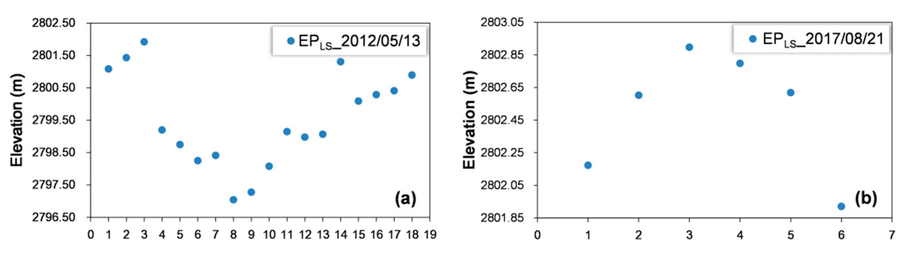
3.2.2. Extraction of the Lake Water Level

Figure 2b shows the extraction of the lake water level and the screening methods. First, the elevation points of the lake were extracted. This study combined three sets of satellite altimetry data. Although the data formats and observation standards differ, the observation principles are basically the same [50,51,52]:
E = alt range + c ,
where E is the distance from the lake surface to the WGS-84 reference ellipsoid, which is called the lake water level in this paper; “alt” is the distance from the satellite to the WGS-84 reference ellipsoid; “range” is the distance from the satellite to the lake surface; and c is the corrections.
In addition, this study used an L2 product. The water level of the lake was calculated; therefore, the corresponding fields of lake water level could be read directly. In addition, to screen the elevation points of the lake, we extracted the longitude, latitude, and collection time of the elevation points. Table 2 shows the corresponding fields of the above data derived from three products.
After determining the fields to be read, the elevation points of the lake surface (EPLS) were obtained by filtering the lake boundary during the dry period, as shown in Figure 3a,b (Sentinel-3, 12 April 2020 period data). The altimeter satellite is mostly based on radar or laser altimeter measurements of the surface; therefore, the data quality is affected by various combinations of factors, such as clouds, rainfall, sand, and lake-surface reflections [35], resulting in scattered elevation points for the lake surface, not all of which are valid, as shown in Figure 3c. This study thus proposes a mean-independent algorithm based on two reasonable assumptions: (1) Gahai Lake is a typical terminal lake, so the water of the lake does not flow out, the lake surface is relatively stable, and the elevation basically remains the same in all places; and (2) the elevation data for the lake surface are normally distributed, which means that the majority of elevation points are correct, and there are only a few abnormal points. Table 3 illustrates the proposed algorithm.
The lake water level for each period was calculated by using the proposed algorithm to process the multisource satellite altimetry data. The number of EPLS and EEPLS in each issue was counted, and the effective rate (ER = EEPLS/EPLS × 100%) was calculated to compare the lake water levels from different periods. Moreover, data with ER and EPLS numbers below a certain threshold were excluded (see Section 4.1.3) from the final results.

3.2.3. Estimation of the Lake Water Storage Changes

Figure 2c outlines the process for estimating lake water storage. After extracting data of the area and water level, those with similar collection dates were selected to form data pairs to establish a hypsographic curve. Linear, exponential, quadratic, and cubic polynomial curves were selected to fit the existing time-matched pairs, and the coefficient of determination (R2) and the root mean square error (RMSE) were used to evaluate how much the curves match the existing data [53].
After establishing the optimized hypsographic curve, the missing water level was predicted from a long time series of area, utilizing water level pairs, which could be used with the PFM to estimate the long-term variations in water storage:
Δ LWS = 1 3 A t + A t + 1 + A t A t + 1 E t + 1 E t
where ∆LWS is the change in lake water storage from time t to time t + 1, At and Et are the area and water level at time t, and At+1 and Et+1 are the lake area and water level at time t + 1.
In addition, the inverse function of E (A) was calculated to obtain A(E), and the IM (4) could be used to estimate the change in water storage of the lake.
Δ LWS = E t E t + 1 A E d E ,
where Et is the water level at t, Et+1 is the water level at t + 1, and A(E) is the inverse function of the hypsographic curve E(A).
It is worth mentioning that in Equations (3) and (4), moment t + 1 is adjacent to moment t; therefore, the two models could estimate the change in water storage only between adjacent moments.

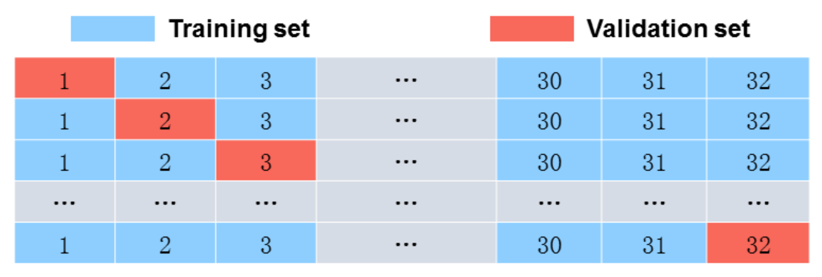
3.2.4. Verification of the Predicted Hypsographic Curve

As discussed in Section 3.2.3, the best fit hypsographic curve to the available data could be selected based on the evaluation index R2 and the RMSE. However, the accuracy of the estimates produced by the curve for data-deficient periods needed to be verified to ensure the long-term water level and water storage of the lake. This paper used cross-validation to verify the accuracy of the hypsographic curve [54]. The basic idea of cross-validation was to divide the original data into a training set and a validation set, and then the training set was used to construct the function to produce the curve. Few time-matched data pairs were available for Gahai Lake; therefore, all the data could be used to validate the function for the hypsographic curve [55]. Leave-one-out cross-validation, which is more applicable to small sample sets, was used in this study [56]. Thirty-two time-matched data pairs were split into 32 sub-samples. Thirty-one sub-samples were used to construct the curve E(A) of water level versus area, and the remaining sub-sample was used to verify the accuracy of the curve. The cross-validation was repeated 32 times because each (area, water level) data pair was used in one validation. Eventually, the absolute error and mean absolute error of the 32 validations served to evaluate the accuracy of the curve. Figure 4 shows the leave-one-out cross-validation configuration.

4. Results and Analysis

4.1. Extraction of the Area and Water Level for Gahai Lake

The extraction results of lake areas and water levels in this study are presented in three sections. Section 4.1.1 compares the lake area extracted from two types of optical images to prove the necessity of using Landsat to extract small lake areas. Section 4.1.2 shows the transit tracks of other altimetry satellites in Gahai, which reveal the scarcity of altimetry data in this region. Section 4.1.3 describes the specific results of the proposed algorithm for extracting lake level and the parameter setting process for eliminating outliers.

4.1.1. Comparison of Gahai Lake Area Extracted from Landsat and MODIS

As shown in Figure 5, the lake area extracted from Landsat and MODIS products over the same periods varied significantly. From 2003 to 2019, the annual lake area extracted by MODIS was 4.47–9.09% larger than that extracted by Landsat, with an average of 6.64%, and the difference became narrow with an increasing lake area (see the green solid line). This result is consistent with that of a previous study [22,57], in which the relative difference in lake area extracted by the two products was closely related to the scale of the lake.
For large lakes, although the lake boundaries extracted by the MODIS and Landsat products did not overlap and the calculated lake areas were different, the dissimilarity was almost negligible compared with the large lake area. In this case, the products could be combined or interchanged in practice [32]. For small lakes, the low spatial resolution of MODIS means that the boundaries of small lakes are difficult to distinguish from surrounding features, forming mixed images; thus, a large uncertainty remained in the extracted lake boundary. In addition, the large difference in spatial resolution between the two products meant that the extracted lake boundaries may have differed by over 200 m, resulting in different calculated areas. The Landsat products provide better spatial resolution, but the time resolution is limited, so they are more suitable for monitoring annual variation in the lake area.

4.1.2. Satellite Altimetry Data for the Area of Gahai Lake

Apart from the three altimetry satellite data in this study, the transits of other altimeter satellites over Gahai Lake can be obtained from the Aviso-CNES data center (https://www.aviso.altimetry.fr/en/data/tools/pass-locator.html, access date: 26 January 2021) (see Figure 6a). Only two tracks transit over Gahai Lake, namely, Jason2_LRO (adjusted from July 2017 to July 2018) and EnviSat_new (after adjusting its orbit in November 2010). Jason2_LRO passed over Gahai Lake three times (orbital numbers cycle501/pass129, cycle524/pass057, and cycle529/pass074, dated 25 July 2017, 6 March 2018, and 25 April 2018, respectively). The observation points (from Jason2_GDR data provided by AVISO) are sparse, and only one point lay in Gahai Lake (see Figure 6b), with a value of 2885.741 m (reference WGS84 ellipsoid), which differed significantly from the other data presented herein. EnviSat_new passed by Gahai Lake only once, and the result was similar to that of Jason2_LRO. In addition, the transits over Gahai Lake by ICESat satellites were also counted (https://nsidc.org/data/GLAH14/versions/34, access date: 27 January 2021), but the results were not recorded. To summarize, except for the altimeter satellite data used in this study, there is little altimeter satellite coverage for the Gahai Lake. This may be the reason why some public datasets (e.g., Hydroweb [58], DAHITI [59], and G-REALM [60]) lack records of the water levels of Gahai Lake.

4.1.3. Extraction of Water Level of Gahai Lake

To extract the initial water level of Gahai Lake and form a time series, the proposed water-level extraction algorithm was used to calculate the data from three altimeter satellites that passed over Gahai Lake (see Figure 7a). The apparent deviation of water level from the data acquired on adjacent dates (see red solid circles) may result from an error in the original lake-elevation point. To further analyze this phenomenon, the number of lake elevation points (N_EPLS), the number of effective lake-elevation points (N_EEPLS), and the percentage of effective lake-elevation points (RE) were collected and compared for all periods of deviation in the water level, as indicated in Table 4. For the 14 periods when the lake water level deviated, there were fewer than 40% of the effective elevation points on the lake surface over 12 periods, which indicates that the original lake-elevation points were widely dispersed (see Figure 8a). There were two periods in which RE > 40%, but few initial lake-elevation points (see Figure 8b). These results suggest that the original lake-elevation points may not be reliable. Therefore, the ER and EPLS in 3.2.2 were set to 40% and 8, respectively, to eliminate these possible anomalous water levels from the time series of lake water levels. In the end, the water level of Gahai Lake was obtained, as shown in Figure 7.

4.2. Hypsographic Curves for Gahai Lake

Given the water level and corresponding area, four hypsographic curves were fitted for Gahai Lake, as shown in Figure 9.
The determination coefficients R2 for the four curves are 0.742, 0.742, 0.766, and 0.802, and the RMSEs are 0.175 m, 0.175 m, 0.167 m, and 0.153 m, respectively. The cubic polynomial curve had the highest coefficient of determination (0.802) and the lowest RMSE (0.153 m), which meant that this curve fitted the data the best. However, when the lake area exceeded 38,730 km2 (see Figure 9d), the water level tended to decrease. Considering the geographical condition of Gahai Lake, there is no situation when if the area increases, the water level decreases. In other words, the hypsographic curve of Gahai Lake increases monotonically. The cubic polynomial curve was excluded because it did not meet this criterion. For the other three curves, the quadratic polynomial curve provided the highest coefficient of determination (0.766) and the lowest RMSE (0.167 m); therefore, this curve was chosen as the optimized hypsographic curve for Gahai Lake:
E A = 0.028 A 2 + 2.307 A + 2754.901 .
The hypsographic curve could not be established given a small range of lake levels because of the inevitable observation errors and limits caused by the data acquisition dates of lake area and water level. There was almost no obvious relationship (neither linear nor nonlinear) between lake area and water level. In other words, the proposed method has difficulty monitoring lakes with small changes in water level (especially when the variation in water level is less than 1 m), which is consistent with the description by Xu et al. [61]. Conversely, lakes with less variation in water level are not the focus of attention.

4.3. Variations in the Area, Water Level and Water Storage of Gahai Lake

4.3.1. Variations in the Area of Gahai Lake

Figure 10 shows the interannual variations in the area of Gahai Lake. From 1975 to 2020, the lake area fluctuated within the range of 28.37–38.57 km2, showing a slightly increasing trend of 0.14 km2/y, and the lake area increased by 20.17% in 45 years. The whole period can be divided into two sub-periods based on the short-term variations in the lake area. In the first sub-period (1975–1999), the lake area contracted: the lake area fluctuated between 32.10 and 28.44 km2 and decreased slightly by 0.15 km2/y. From 1975 to 1987, the lake area decreased at a rate of 0.29 km2/y for a total of 3.53 km2. It entered a short period of expansion, during which the lake area increased by 1.69 km2 at a rate of 0.34 km2/y. The lake again entered a period of decreasing area in 1992, when it shrank at a rate of 0.26 km2/y until reaching a minimum area of 28.44 km2 in 1999. In the second sub-period (2000–2020), the lake expanded by 9.74 km2 at a rate of 0.49 km2/y. During this period, the lake area expanded from 2001 to 2013 for 12 consecutive years. It increased by 6.71 km2, which was equal to 23.65% of the lake area in 2001, at an increasing rate of 0.56 km2/y. From 2013 to 2016, the lake area contracted slightly by 0.28 km2 at a rate of 0.09 km2/y. In 2016, the lake entered a period of rapid increase, which had never happened over the past 45 years. By 2020, the lake area had increased by 3.78 km2, with an increasing rate of 0.94 km2/y, which significantly exceeded the rates (increasing or decreasing) of all other periods.
To summarize, during the first sub-period (1975–1999), the lake area was decreasing slightly. During the second sub-period (2000–2020), the lake area increased at a relatively high rate, especially in recent years. The high increasing rate in the lake area (up to threefold greater than the previous period) distinguishes the later period from the previous one.
Figure 11 shows the spatial variations in the lake area. During the first sub-period, the lake area only varied slightly at the boundary, with relatively larger variations in the north and southeast regions. During the second sub-period, the lake area changed significantly compared with the first sub-period, with large expansions in the north, south, and southeast parts of the lake, but there is only little variation in the northeast part of the lake. Optical images and a digital elevation model of the lake area show that the northeast part of the lake is dominated by a cliff, so very little variation in this area can be seen unless the water level increases significantly. In short, due to the steep slope in the northeast part of the lake, the lake area in this region remains unchanged despite the fluctuation of the water level, whereas the slopes in other parts of the lake are relatively small and therefore are more prone to significant variations in lake area.

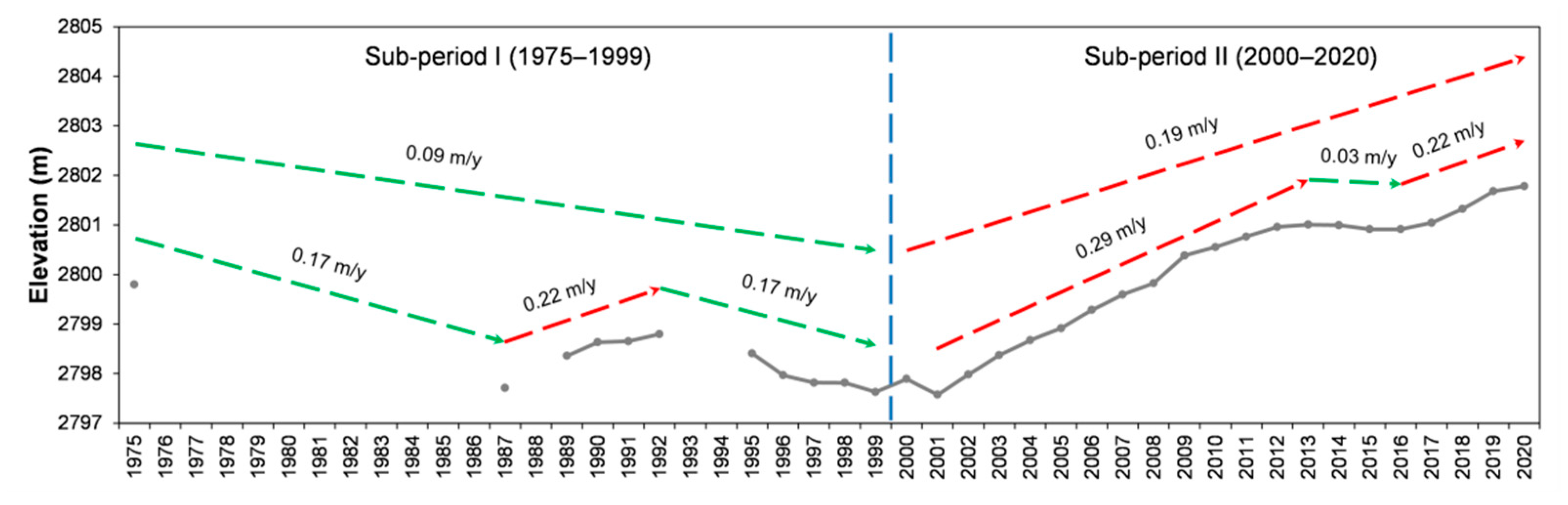
4.3.2. Variations in the Water Level of Gahai Lake

Based on the variations in lake area from 1975 to 2020 in Section 4.3.1, a quadratic polynomial was adopted as the optimum curve to describe the water level of the lake over this period. Figure 12 shows the interannual variation in the water level of Gahai Lake.
From 1975 to 2020, the water level fluctuated between 2797.58 m and 2801.79 m, showing a slight upward trend of 0.04 m/y on average. Similarly, the whole period can be divided into two sub-periods based on short-term variations in water level. During the first sub-period (1975–1999), the water level decreased from 2799.80 m to 2797.63 m, at a rate of 0.09 m/y. From 1975 to 1987, the water level dropped by 2.09 m, at a decreasing rate of 0.17 m/y. From 1987 to 1992, the water level increased by 1.08 m at a rate of 0.22 m/y. From 1992 to 1999, the water level again declined at a rate of 0.17 m/y to reach a minimum of 2797.63 m in 1999.
During the second sub-period (2000–2020), the water level increased by 3.89 m at an average rate of 0.19 m/y. From 2001 to 2013, the water level grew monotonically at 0.29 m/y, with a total increase of 3.43 m, which accounted for 88.18% of the total increase in the second sub-period. The water level saw a relatively rapid increase during these 12 years. From 2013 to 2016, the water level remained almost stable, with only a slight decrease of 0.09 m over these three years (0.03 m/y). From 2016 to 2020, the water level rose at 0.22 m/y for a total increase of 0.87 m, which was similar to the growth in other periods, whereas the lake area in the same period increased rapidly compared with that in other periods. This shows that even within the same period, variations in the lake area and the water level may be different.
Figure 13 shows how lake area and water level vary over different periods. From 2016 to 2020, the increasing rates in the area were 2.76 times and 1.68 times greater than those from 1987 to 1992 and from 2001 to 2013, respectively. The analogous comparison for water level gives factors of 1.00 and 0.76, respectively. These results indicate that the significant increase in area from 2016 to 2020 resulted from only a small increase in water level. Thus, the area and water level are only single indicators of variations in lake water resources, and any analysis of lake properties based solely on an area or on water level is incomplete. In this particular case, different indicators may lead to completely different conclusions when the lake has a high water level or large area. Therefore, it is estimated that the variations in water storage directly influence the water resources of the lake.

4.3.3. Variations in Water Storage of Gahai Lake

Given the data on lake area and water level from 1975 to 2020, the pyramidal frustum model and integral model were adopted to estimate the variations in water storage of the lake during this period. Figure 14 shows the change in water storage estimated by the two models (blue and red curves) and the difference between the two models (gray histogram). The results of the pyramidal frustum model and the integral model show that over the 45 years, water storage increased by 68.79 × 10⁶ m3 and 82.33 × 10⁶ m3, which give rates of 1.53 × 10⁶ m3/y and 1.83 × 10⁶ m3/y, respectively. Compared with the result gained from the integral model, water storage saw a less significant increase over 45 years in the pyramidal frustum model. With respect to the water storage level in 1975 (arbitrarily set to zero), the pyramidal frustum model estimated that the water storage first decreased to a minimum of −67.15 × 10⁶ m3 in 2001, and then rose to a maximum of 68.79 × 10⁶ m3 in 2020. The analogous numbers for the integral model were −93.30 and 82.33 × 10⁶ m3, respectively. To summarize, the water-storage trends estimated by the two models were similar, but the specific values differed.
This difference may be explained by the fact that the two models are based on different principles for estimating variations in water storage. The pyramidal frustum model regards the variation in water storage as the volume of a regular prism, whereas the actual lake basin has an irregular shape, which leads to greater uncertainty in the resulting estimation. The integral model regards the variation in water storage as the limit of the integral of the lake-area function over a certain water level interval, which is theoretically more rigorous than the pyramidal frustum model, but it is limited by the accuracy of the hypsographic curve. Given the lack of in situ measurement data on water storage, it is impossible to objectively assess the results of these models. The mean value of the two results was used as the final changes in lake water storage to balance the contributions of the two models, as shown in Figure 15.
Over the period 1975–2020, water storage in Gahai Lake increased by approximately 75.56 × 10⁶ m3, at an increasing rate of 1.68 × 10⁶ m3/y. The whole period was again divided into two sub-periods, in the first of which (1975–1999) water storage varied more drastically, decreasing at an average of 3.26 × 10⁶ m3/y. During the period 1975–1987, water storage fell by 75.38 × 10⁶ m3 (−6.28 × 10⁶ m3/y). In the following five years, water storage increased by 38.72 × 10⁶ m3 (+7.74 × 10⁶ m3/y). From 1992 to 1999, water storage again dropped by 41.68 × 10⁶ m3 (−5.95 × 10⁶ m3/y).
The second sub-period (2000–2020) saw a steady increase in water storage. It increased by 1.45 × 10⁶ m3 (+7.23 × 10⁶ m3/y). From 2001 to 2013, water storage increased for 12 consecutive years, with a total increase of 1.25 × 10⁶ m3 (+10.46 × 10⁶ m 3/y). The water storage in 2008 was the same as in 1975. From 2013 to 2016, the water storage changed slightly, decreasing by 3.52 × 10⁶ m3 (−1.17 × 10⁶ m3/y). During the period 2016–2020, water storage rose by 33.82 × 10⁶ m3 (+8.45 × 10⁶ m3/y), which was slower than that from 2001 to 2013, but similar to the growth rate from 1987 to 1992. These results differ from those for the area and water level of the lake during the same period, which again confirms the conclusion drawn in Section 4.3.2.

5. Discussion

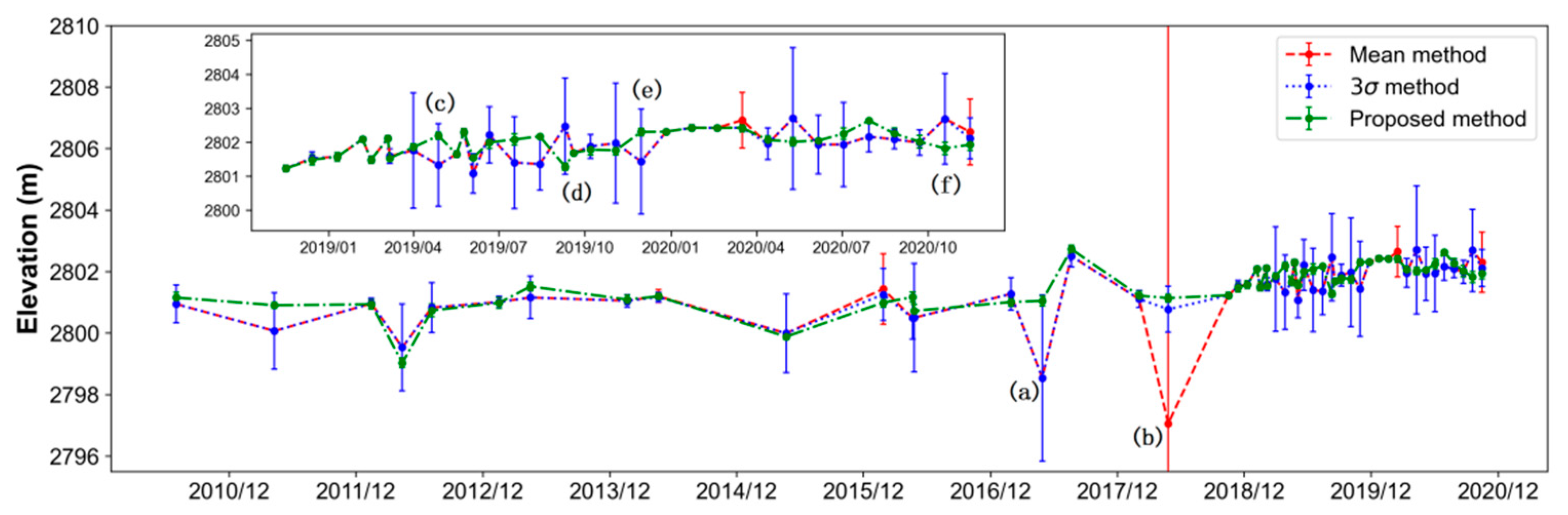
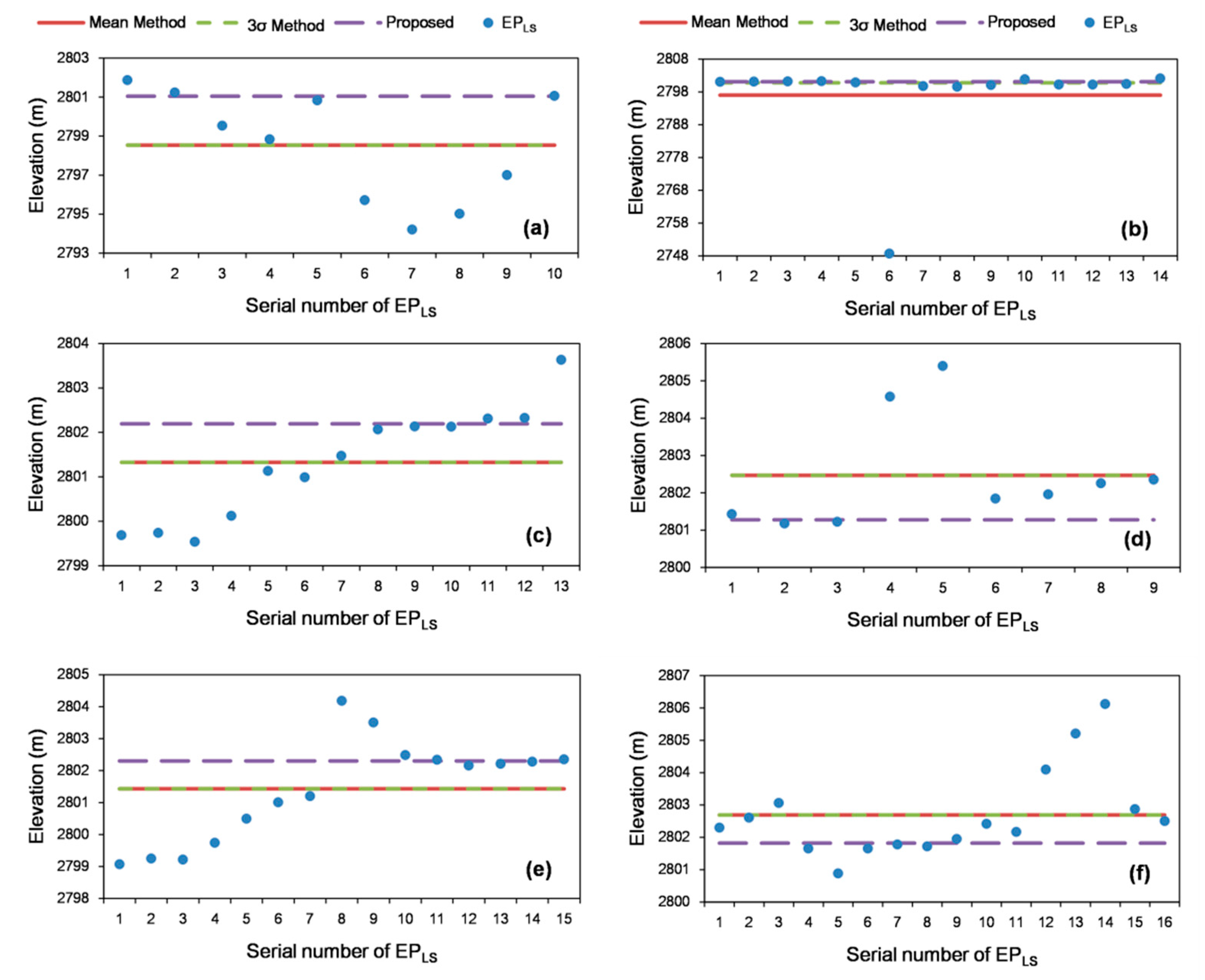
5.1. Rationalization for the Extraction of Water Level of the Lake

Figure 16 shows the water levels of lakes extracted using the mean method, the 3σ method, and the proposed algorithm. The water levels for each period are given by the mean and standard deviation of the set of lake elevation points run by the given method. The water level based on the point set processed by the proposed method had the smallest standard deviation (0.12 m); the mean method and the 3σ method produced standard deviations of 0.97 m and 0.69 m, respectively, which were significantly greater than that of the proposed method. The overall water level of the lake was generally consistent among the three methods, but large differences did exist on specific dates. The six most controversial water-level points were selected to analyze this difference (see Figure 17).
The results extracted by the mean method and the 3σ method were almost the same (red dashed line and green dashed line), but were significantly affected by outliers. When outliers strongly differed from other elevation points, the extraction results of the mean method deviated from the expected value (see Figure 17b). The 3σ method can eliminate the most egregious outliers, although it has difficulty eliminating minor ones (i.e., deviations of 1–5 m; see Figure 17a,c–f). The results of the 3σ method were the same as those of the mean method, which indicates that the outliers were not eliminated, but rather counted in the calculation of the water level. In addition, the 3σ method and the mean method were difficult to apply to small lakes. Large lakes often have a sufficient number of lake elevation points; therefore, the 3σ method can easily eliminate the most prominent outliers using the mean value as a reference, and the mean method can rely on sufficient points to offset the outliers. However, for small lakes such as Gahai Lake, only a small number of lake elevation points are available because of the small lake area and the configuration of the orbits of altimeter satellites. This small number of lake elevation points leads to more randomly distributed outliers due to the influence of cloud cover, the reflection of the land–water boundary [35], and other factors (see Figure 17a,b,d,f). Given the small number of lake elevation points, taking the mean cannot offset these outliers. The 3σ method is also unreliable in this case because the mean value deviates from the expected value. Although the threshold of this method can be adjusted to σ or 2σ, selecting the threshold can be very complicated because of the different values of the outlying lake elevation points.
Based on the two assumptions of the proposed method, the largest set of elevation points in a certain elevation range (the fluctuation of water level in Gahai Lake was relatively stable in a single measurement; thus, the range of elevation was selected as ±0.3 m) was considered as the effective set of elevation points of the lake. The observation did not contain outliers because outlier points are relatively independent and randomly distributed, and therefore are rarely clustered within a certain range of elevation. The proposed method is thus more suitable for extracting the water level of small lakes.

5.2. Validation of the Hypsographic Curve

To justify the water level and water storage of lakes estimated by the quadratic polynomial curve, the accuracy of the hypsographic curve was explored by using the leave-one-out cross-validation method in Section 3.2.4
Figure 18 shows the results of the leave-one-out cross-validation of various hypsographic curves. The x-axis shows the area from the time-matched data pairs used for testing, and the y-axis shows the value of absolute error in water level (for ease of analysis). The results are divided into four sections based on the trend of the absolute error of the curve for a given area. In the first section (34.60–35.78 km2), the linear curve (blue solid line) and exponential curve (red dashed line) produce the smallest mean absolute error (0.066 m), followed by the quadratic polynomial curve (0.077 m), and the cubic polynomial curve (0.092 m). In the second section (35.78–36.49 km2), the cubic polynomial curve gives the smallest mean absolute error (0.076 m), followed by the linear and exponential curves (0.114 m) and then the quadratic polynomial curve (0.123 m). In the third section (36.49–37.02 km2), both the linear and exponential curves give mean absolute errors of 0.188 m, and the other two curves give 0.193 m. In the fourth section (37.02–39.55 km2), the cubic polynomial curve gives the smallest mean absolute error (0.176 m), followed by the quadratic polynomial curve (0.189 m), the linear curve (0.197 m), and the exponential curve (0.197 m). In addition, over the entire range of lake-area values (34.60–39.55 km2), the smallest mean absolute error was produced by the cubic polynomial curve (0.146 m), followed by the quadratic polynomial curve (0.157 m), the linear curve (0.158 m), and the exponential curve (0.158 m).
To summarize, the cubic polynomial curve produced the most accurate estimate of area or water level, followed by the quadratic polynomial curve, the exponential curve, and the linear curve. However, the cubic polynomial curve did not match the geography condition of Gahai Lake; therefore, the quadratic polynomial curve was used to estimate the area or water level of the lake in periods devoid of data.

5.3. Discussion of Variations in Water Storage of Gahai Lake

Figure 19 shows the annual water storage in Gahai Lake from 2001 to 2020 and as a function of annual precipitation at the lake, annual runoff volume, and annual variation in cropland relative to 2001. Figure 19a shows that the annual precipitation fluctuated significantly over the years, with a slight overall increase, whereas the annual water storage of the lake increased monotonically over the same period. The two trends show different patterns. The correlation coefficient between the two datasets was R = 0.15 and the significance level was p > 0.1, which indicates that no correlation existed between the two sets (see Figure 19b). Similar results were obtained for annual variation in runoff volume (see Figure 19c), which also showed no correlation with water storage (R = 0.24, p > 0.1; see Figure 19d). Moreover, the annual variation in cropland in the upper lake region and the annual variation in lake water storage both exhibited a long period of monotonic increase (see Figure 19e); thus, the two are strongly correlated (R = 0.76, p < 0.01; see Figure 19f).
Over the past 20 years, precipitation in the lake and runoff from the Bayin River basin have had little effect on the variations in water storage in the lake; therefore, the cropland area appears to be the main factor contributing to variations in the water storage of the lake. This effect is indirect because a variation in the cropland area will lead to a variation in irrigation volume. Given that heavy irrigation is applied to the area, a variation in cropland area will produce a proportional variation in the amount of receding irrigation water that flows into the lake as subsurface and surface runoff, which then affects the water storage in the lake. In recent years, in particular, the water storage has increased at a higher rate than previous years, reflecting the rapid increase in cropland area and the concomitant irrigation withdrawal in upstream areas, which leads to a serious waste of local agricultural water. Therefore, more scientific irrigation methods should be adopted to ensure the efficient and appropriate use of agricultural water.

6. Conclusions

The combination of multisource data proves to be a feasible way to detect variations in small lakes at low and middle latitudes. This study estimated variations in the area, water level, and water storage of the Gahai Lake from 1975 to 2020 and analyzed the related trends and the physical mechanisms that give rise to these trends. The results show that the area and water level of Gahai Lake have increased over the past 45 years, but in recent years, the trends of the two indicators are significantly different. This not only reflects the topographic characteristics of the Gahai Lake basin, but also indicates that it is difficult to accurately determine the variations in lakes based on lake area or water level alone. Instead, water storage has proven to be the most direct and accurate indicator.
The water level of relatively small lakes such as the Gahai Lake is difficult to be accurately determined because it offers few elevation points and a high proportion of outliers. To overcome this problem, this study proposes an algorithm to extract the effective elevation points of the lake without relying on their mean value, and it is shown that this algorithm can accurately extract the water level of the lake. In addition, the altimeter-satellite revisit time left some periods with few or no data; therefore, the existing time-matched data pairs had to be used to fill in these gaps. Four different functions were applied to the existing data and they were tested to find out which one provides the best estimate of water level versus area in the periods with little or no data. These trials show that a quadratic polynomial method can best estimate the hypsographic curve for Gahai Lake. Water level, as a function of area, reflects the shape of the lake basin to some extent, and this function may differ for different types of lakes. Therefore, it is recommended that the function used to estimate water level versus area should be thoroughly investigated before using it to estimate variations in water storage in lakes to ensure its optimality.
Two models were used to estimate the water storage changes of Gahai Lake, and the differences in the results were discussed. The results show that the water storage trends of Gahai Lake estimated by the two models were similar, but there were large differences in the values, which may be due to different principles of the two models. The pyramidal frustum model was difficult to fit to the actual lake basin shape; thus, the reliability of the results was low. The integral model is theoretically more rigorous, but it was limited by the accuracy of the hypsographic curve. No in situ measurement data were available for verification; therefore, the mean value of the two results was used as the final changes in lake water storage to balance the contributions of the two models. Finally, we believe that analyzing the results of different models and fully considering the contributions of all results is an effective way to estimate the changes in lake water storage in ungauged regions.
Hypsographic curves (lake area versus water level) are indispensable for predicting lake areas or water levels in some periods and for estimating variations in water storage in lakes by applying prismatic or integral models. However, due to the launch time and orbit configuration of optical remote-sensing satellites and altimeter satellites, the time-matched (lake area, water level) data pairs are temporally insufficient. The problem is expected to be overcome in the future when NASA launches surface water and ocean topography (SWOT) tasks in 2022 (https://swot.jpl.nasa.gov/, access date: 15 April 2021), which will carry sensors that can capture both the water level and area of lakes, and obtain data pairs with almost perfect temporal correlation, thereby greatly improving the accuracy by which water level versus area may be determined [62]. This will greatly improve the accuracy of estimated variations in water storage in lakes. Therefore, it will be possible to develop accurate remote-sensing monitoring of variations in water storage in small lakes such as the Gahai Lake in the near future. However, the long time-series data of variations in the area, water level, and water storage will still rely on imperfect data provided by the previous missions (e.g., Landsat, CryoSat) for some time. Moreover, the joint application of conventional data and SWOT data, and their inter-validation, may be an issue worth investigating in the future.
The analysis of water storage changes in the Gahai Lake indicates that a key contributing factor to these variations is the irrigation withdrawal from the upper reaches of the Gahai Lake over the past 20 years. The expanding irrigation of this cropland area and the concomitant rise in irrigation runoff appear to be the main contributor to the increase in water storage in Gahai Lake. This phenomenon reveals the inefficient use of agricultural water that results from crude heavy irrigation. Therefore, it is suggested that local authorities should improve the irrigation methods used on cropland to ensure the efficient and appropriate use of agricultural water.

Author Contributions

Conceptualization, C.Z., A.L. and G.Y.; methodology, C.Z. and G.Y.; formal analysis, C.Z.; visualization, C.Z. and G.Y.; validation, W.Z. and S.Q.; writing—original draft preparation, C.Z.; writing—review and editing, A.L., W.Z., G.Y. and S.Q.; supervision, A.L., W.Z. and G.Y.; project administration and funding acquisition, A.L. All authors have read and agreed to the published version of the manuscript.

Funding

This research was funded the Important Science & Technology Specific Projects of Qinghai Province (2019-SF-A4-1), the National Natural Science Foundation of Qinghai Province (2019-ZJ-7020) and the National Natural Science Foundation of China (41671026).

Acknowledgments

We would like to thank the editors and anonymous reviewers for their constructive comments and suggestions. Thanks also go to the teams at NASA, ESA and Copernicus who have made their datasets available and use for free.

Conflicts of Interest

The authors declare no conflict of interest.

References

  1. Liu, B.; Wang, Y.; Xia, J.; Quan, J.; Wang, J. Optimal water resources operation for rivers-connected lake under uncertainty. J. Hydrol. 2021, 595, 125863. [Google Scholar] [CrossRef]
  2. Zhu, W.; Yan, J.; Jia, S. Monitoring recent fluctuations of the southern Pool of Lake Chad using multiple remote sensing data: Implications for water balance analysis. Remote Sens. 2017, 9, 1032. [Google Scholar] [CrossRef] [Green Version]
  3. Che, X.; Feng, M.; Sun, Q.; Sexton, J.O.; Channan, S.; Liu, J. The Decrease in Lake Numbers and Areas in Central Asia Investigated Using a Landsat-Derived Water Dataset. Remote Sens. 2021, 13, 1032. [Google Scholar] [CrossRef]
  4. Song, C.; Huang, B.; Ke, L.; Richards, K.S. Remote sensing of alpine lake water environment changes on the Tibetan Plateau and surroundings: A review. ISPRS J. Photogramm. Remote Sens. 2014, 92, 26–37. [Google Scholar] [CrossRef]
  5. Qiao, B.; Zhu, L.; Yang, R. Temporal-spatial differences in lake water storage changes and their links to climate change throughout the Tibetan Plateau. Remote Sens. Environ. 2019, 222, 232–243. [Google Scholar] [CrossRef]
  6. Qiao, B.; Zhu, L.; Wang, J.; Ju, J.; Ma, Q.; Huang, L.; Chen, H.; Liu, C.; Xu, T. Estimation of lake water storage and changes based on bathymetric data and altimetry data and the association with climate change in the central Tibetan Plateau. J. Hydrol. 2019, 578, 124052. [Google Scholar] [CrossRef]
  7. Zhang, G.; Chen, W.; Li, G.; Yang, W.; Yi, S.; Luo, W. Lake water and glacier mass gains in the northwestern Tibetan Plateau observed from multi-sensor remote sensing data: Implication of an enhanced hydrological cycle. Remote Sens. Environ. 2020, 237, 111554. [Google Scholar] [CrossRef]
  8. Jiao, J.J.; Zhang, X.; Liu, Y.; Kuang, X. Increased Water Storage in the Qaidam Basin, the North Tibet Plateau from GRACE Gravity Data. PLoS ONE 2015, 10, e0141442. [Google Scholar] [CrossRef] [Green Version]
  9. Jiao, K.; Gao, J.; Liu, Z. Precipitation Drives the NDVI Distribution on the Tibetan Plateau While High Warming Rates May Intensify Its Ecological Droughts. Remote Sens. 2021, 13, 1305. [Google Scholar] [CrossRef]
  10. Lv, A.; Zhou, L. A Rainfall Model Based on a Geographically Weighted Regression Algorithm for Rainfall Estimations over the Arid Qaidam Basin in China. Remote Sens. 2016, 8, 311. [Google Scholar] [CrossRef] [Green Version]
  11. Zhao, L.; Wang, X.; Ma, Y.; Li, S.; Wang, L. Investigation and assessment of ecological water resources in the salt marsh area of a salt lake: A case study of West Taijinar Lake in the Qaidam Basin, China. PLoS ONE 2021, 16, e0245993. [Google Scholar]
  12. Qi, S.; Lv, A. Applicability analysis of multiple precipitation products in the Qaidam Basin, Northwestern China. Environ. Sci. Pollut. Res. Int. 2021, 1–17. [Google Scholar] [CrossRef]
  13. Birkett, C.M. The contribution of TOPEX/POSEIDON to the global monitoring of climatically sensitive lakes. J. Geophys. Res. 1995, 100, 25179. [Google Scholar] [CrossRef]
  14. Li, S.; Chen, J.; Xiang, J.; Pan, Y.; Huang, Z.; Wu, Y. Water level changes of Hulun Lake in Inner Mongolia derived from Jason satellite data. J. Vis. Commun. Image Represent. 2019, 58, 565–575. [Google Scholar] [CrossRef]
  15. Jiang, L.; Nielsen, K.; Andersen, O.B.; Bauer-Gottwein, P. Monitoring recent lake level variations on the Tibetan Plateau using CryoSat-2 SARIn mode data. J. Hydrol. 2017, 544, 109–124. [Google Scholar] [CrossRef] [Green Version]
  16. Xu, X.; Yuan, L.; Jiang, Z.; Chen, C.; Cheng, S. Lake level changes determined by Cryosat-2 altimetry data and water-induced loading deformation around Lake Qinghai. Adv. Space Res. 2020, 66, 2568–2582. [Google Scholar] [CrossRef]
  17. Liao, J.; Liao, J.; Shen, G.; Zhao, Y.; Zhao, Y. Dataset of Global Lake Level Changes Using Multi-altimeter Data (2002-2016). J. Glob. Chang. Data Discov. 2018, 2, 295–302. [Google Scholar] [CrossRef]
  18. Wen, J.; Zhao, H.; Jiang, Y.; Chen, D.; Ji, G. Research on the quality screening method for satellite altimetry data—Take Jason-3 data and Hongze Lake as an example. South North Water Transf. Water Sci. Technol. 2018, 16, 194–200+208. [Google Scholar] [CrossRef]
  19. Feng, L.; Hu, C.; Chen, X.; Cai, X.; Tian, L.; Gan, W. Assessment of inundation changes of Poyang Lake using MODIS observations between 2000 and 2010. Remote Sens. Environ. 2012, 121, 80–92. [Google Scholar] [CrossRef]
  20. McCullough, I.M.; Loftin, C.S.; Sader, S.A. High-frequency remote monitoring of large lakes with MODIS 500m imagery. Remote Sens. Environ. 2012, 124, 234–241. [Google Scholar] [CrossRef]
  21. Pekel, J.F.; Cottam, A.; Gorelick, N.; Belward, A.S. High-resolution mapping of global surface water and its long-term changes. Nature 2016, 540, 418–422. [Google Scholar] [CrossRef]
  22. Wang, J.; Sheng, Y.; Tong, T.S.D. Monitoring decadal lake dynamics across the Yangtze Basin downstream of Three Gorges Dam. Remote Sens. Environ. 2014, 152, 251–269. [Google Scholar] [CrossRef]
  23. Zhang, B.; Wu, Y.; Zhu, L.; Wang, J.; Li, J.; Chen, D. Estimation and trend detection of water storage at Nam Co Lake, central Tibetan Plateau. J. Hydrol. 2011, 405, 161–170. [Google Scholar] [CrossRef]
  24. Seyoum, W.M. Characterizing water storage trends and regional climate influence using GRACE observation and satellite altimetry data in the Upper Blue Nile River Basin. J. Hydrol. 2018, 566, 274–284. [Google Scholar] [CrossRef]
  25. Schwatke, C.; Dettmering, D.; Seitz, F. Volume Variations of Small Inland Water Bodies from a Combination of Satellite Altimetry and Optical Imagery. Remote Sens. 2020, 12, 1606. [Google Scholar] [CrossRef]
  26. Wang, L.; Kaban, M.K.; Thomas, M.; Chen, C.; Ma, X. The Challenge of Spatial Resolutions for GRACE-Based Estimates Volume Changes of Larger Man-Made Lake: The Case of China’s Three Gorges Reservoir in the Yangtze River. Remote Sens. 2019, 11, 99. [Google Scholar] [CrossRef] [Green Version]
  27. Liu, Y.; Yue, H. Estimating the fluctuation of Lake Hulun, China, during 1975-2015 from satellite altimetry data. Environ. Monit. Assess. 2017, 189, 630. [Google Scholar] [CrossRef] [PubMed]
  28. Baup, F.; Frappart, F.; Maubant, J. Combining high-resolution satellite images and altimetry to estimate the volume of small lakes. Hydrol. Earth Syst. Sci. 2014, 18, 2007–2020. [Google Scholar] [CrossRef] [Green Version]
  29. Abileah, R.; Vignudelli, S.; Scozzari, A. A completely remote sensing approach to monitoring reservoirs water volume. Int. Water Technol. J. 2011, 1, 59–72. [Google Scholar]
  30. Busker, T.; de Roo, A.; Gelati, E.; Schwatke, C.; Adamovic, M.; Bisselink, B.; Pekel, J.-F.; Cottam, A. A global lake and reservoir volume analysis using a surface water dataset and satellite altimetry. Hydrol. Earth Syst. Sci. 2019, 23, 669–690. [Google Scholar] [CrossRef] [Green Version]
  31. Chen, T.; Song, C.; Ke, L.; Wang, J.; Liu, K.; Wu, Q. Estimating seasonal water budgets in global lakes by using multi-source remote sensing measurements. J. Hydrol. 2021, 593, 125781. [Google Scholar] [CrossRef]
  32. Xu, Y.; Li, J.; Wang, J.; Chen, J.; Liu, Y.; Ni, S.; Zhang, Z.; Ke, C. Assessing water storage changes of Lake Poyang from multi-mission satellite data and hydrological models. J. Hydrol. 2020, 590, 125229. [Google Scholar] [CrossRef]
  33. Yao, F.; Wang, J.; Yang, K.; Wang, C.; Walter, B.A.; Crétaux, J.-F. Lake storage variation on the endorheic Tibetan Plateau and its attribution to climate change since the new millennium. Environ. Res. Lett. 2018, 13, 064011. [Google Scholar] [CrossRef]
  34. Lin, Y.; Li, X.; Zhang, T.; Chao, N.; Yu, J.; Cai, J.; Sneeuw, N. Water Volume Variations Estimation and Analysis Using Multisource Satellite Data: A Case Study of Lake Victoria. Remote Sens. 2020, 12, 3052. [Google Scholar] [CrossRef]
  35. Dettmering, D.; Ellenbeck, L.; Scherer, D.; Schwatke, C.; Niemann, C. Potential and Limitations of Satellite Altimetry Constellations for Monitoring Surface Water Storage Changes—A Case Study in the Mississippi Basin. Remote Sens. 2020, 12, 3320. [Google Scholar] [CrossRef]
  36. Yao, F.; Wang, J.; Wang, C.; Crétaux, J.-F. Constructing long-term high-frequency time series of global lake and reservoir areas using Landsat imagery. Remote Sens. Environ. 2019, 232, 111210. [Google Scholar] [CrossRef]
  37. Håkanson, L. On Lake Form, Lake Volume and Lake Hypsographic Survey. Geogr. Annaler. Ser. A Phys. Geogr. 1977, 59, 1–30. [Google Scholar] [CrossRef]
  38. Huang, J.; Tao, H.; Wang, Y.; Bai, y. Analysis on relationship between water level and water area of lake based on MODIS image. Trans. Chin. Soc. Agric. Eng. 2012, 28, 140–146. [Google Scholar] [CrossRef]
  39. Wang, J.; Yang, S.; Liu, H.; Wang, P.; Lou, H.; Gong, T. Simulation of Lake Water Volume in Ungauged Terminal Lake Basin Based on Multi-Source Remote Sensing. Remote Sens. 2021, 13, 697. [Google Scholar] [CrossRef]
  40. Chaudhari, S.; Felfelani, F.; Shin, S.; Pokhrel, Y. Climate and anthropogenic contributions to the desiccation of the second largest saline lake in the twentieth century. J. Hydrol. 2018, 560, 342–353. [Google Scholar] [CrossRef]
  41. Gou, Z.; Liu, F. Gahai Lake, Qinghai-Tibet Plateau(Delingha), China. J. Glob. Chang. Data Discov. 2018, 2, 456–457. [Google Scholar] [CrossRef]
  42. Zhang, G.; Li, J.; Zheng, G. Lake-area mapping in the Tibetan Plateau: An evaluation of data and methods. Int. J. Remote Sens. 2016, 38, 742–772. [Google Scholar] [CrossRef]
  43. Xu, R.; Tian, F.; Yang, L.; Hu, H.; Lu, H.; Hou, A. Ground validation of GPM IMERG and TRMM 3B42V7 rainfall products over southern Tibetan Plateau based on a high-density rain gauge network. J. Geophys. Res. Atmos. 2017, 122, 910–924. [Google Scholar] [CrossRef]
  44. Jurík, Ľ.; Halászová, K.; Pokrývková, J.; Rehák, Š. Irrigation of Arable Land in Slovakia: History and Perspective. In Water Resources in Slovakia: Part I: Assessment and Development; Negm, A.M., Zeleňáková, M., Eds.; Springer International Publishing: Cham, Switzerland, 2019; pp. 81–96. [Google Scholar]
  45. Liang, D.; Zuo, Y.; Huang, L.; Zhao, J.; Teng, L.; Yang, F. Evaluation of the Consistency of MODIS Land Cover Product (MCD12Q1) Based on Chinese 30 m GlobeLand30 Datasets: A Case Study in Anhui Province, China. ISPRS Int. J. Geo-Inf. 2015, 4, 2519–2541. [Google Scholar] [CrossRef] [Green Version]
  46. Chen, J.; Zhu, X.; Vogelmann, J.E.; Gao, F.; Jin, S. A simple and effective method for filling gaps in Landsat ETM+ SLC-off images. Remote Sens. Environ. 2011, 115, 1053–1064. [Google Scholar] [CrossRef]
  47. Mahajan, S.; Martinez, J. Water, water, but not everywhere: Analysis of shrinking water bodies using open access satellite data. Int. J. Sustain. Dev. World Ecol. 2020, 28, 326–338. [Google Scholar] [CrossRef]
  48. Gu, Z.; Zhang, Y.; Fan, H. Mapping inter- and intra-annual dynamics in water surface area of the Tonle Sap Lake with Landsat time-series and water level data. J. Hydrol. 2021, 601, 126644. [Google Scholar] [CrossRef]
  49. Gao, B.-C. NDWI—A normalized difference water index for remote sensing of vegetation liquid water from space. Remote Sens. Environ. 1996, 58, 257–266. [Google Scholar] [CrossRef]
  50. Nielsen, K.; Stenseng, L.; Andersen, O.B.; Villadsen, H.; Knudsen, P. Validation of CryoSat-2 SAR mode based lake levels. Remote Sens. Environ. 2015, 171, 162–170. [Google Scholar] [CrossRef] [Green Version]
  51. Markus, T.; Neumann, T.; Martino, A.; Abdalati, W.; Brunt, K.; Csatho, B.; Farrell, S.; Fricker, H.; Gardner, A.; Harding, D.; et al. The Ice, Cloud, and land Elevation Satellite-2 (ICESat-2): Science requirements, concept, and implementation. Remote Sens. Environ. 2017, 190, 260–273. [Google Scholar] [CrossRef]
  52. Donlon, C.; Berruti, B.; Buongiorno, A.; Ferreira, M.H.; Féménias, P.; Frerick, J.; Goryl, P.; Klein, U.; Laur, H.; Mavrocordatos, C.; et al. The Global Monitoring for Environment and Security (GMES) Sentinel-3 mission. Remote Sens. Environ. 2012, 120, 37–57. [Google Scholar] [CrossRef]
  53. Li, Y.; Gao, H.; Zhao, G.; Tseng, K.-H. A high-resolution bathymetry dataset for global reservoirs using multi-source satellite imagery and altimetry. Remote Sens. Environ. 2020, 244, 111831. [Google Scholar] [CrossRef]
  54. Shao, J. Linear Model Selection by Cross-validation. J. Am. Stat. Assoc. 1993, 88, 486–494. [Google Scholar] [CrossRef]
  55. Hawkins, D.M.; Basak, S.C.; Mills, D. Assessing model fit by cross-validation. J. Chem. Inf. Comput. Sci. 2003, 43, 579–586. [Google Scholar] [CrossRef] [PubMed]
  56. Vehtari, A.; Gelman, A.; Gabry, J. Practical Bayesian model evaluation using leave-one-out cross-validation and WAIC. Stat. Comput. 2016, 27, 1413–1432. [Google Scholar] [CrossRef] [Green Version]
  57. Chipman, J. A Multisensor Approach to Satellite Monitoring of Trends in Lake Area, Water Level, and Volume. Remote Sens. 2019, 11, 158. [Google Scholar] [CrossRef] [Green Version]
  58. Crétaux, J.F.; Arsen, A.; Calmant, S.; Kouraev, A.; Vuglinski, V.; Bergé-Nguyen, M.; Gennero, M.C.; Nino, F.; Abarca Del Rio, R.; Cazenave, A.; et al. SOLS: A lake database to monitor in the Near Real Time water level and storage variations from remote sensing data. Adv. Space Res. 2011, 47, 1497–1507. [Google Scholar] [CrossRef]
  59. Schwatke, C.; Dettmering, D.; Bosch, W.; Seitz, F. DAHITI—An innovative approach for estimating water level time series over inland waters using multi-mission satellite altimetry. Hydrol. Earth Syst. Sci. 2015, 19, 4345–4364. [Google Scholar] [CrossRef] [Green Version]
  60. Birkett, C.; Reynolds, C.; Beckley, B.; Doorn, B. From research to operations: The USDA global reservoir and lake monitor. In Coastal Altimetry; Springer: Berlin/Heidelberg, Germany, 2011; pp. 19–50. [Google Scholar]
  61. Xu, N.; Ma, Y.; Zhang, W.; Wang, X.H.; Yang, F.; Su, D. Monitoring Annual Changes of Lake Water Levels and Volumes over 1984–2018 Using Landsat Imagery and ICESat-2 Data. Remote Sens. 2020, 12, 4004. [Google Scholar] [CrossRef]
  62. Biancamaria, S.; Lettenmaier, D.P.; Pavelsky, T.M. The SWOT mission and its capabilities for land hydrology. Surv. Geophys. 2016, 37, 307–337. [Google Scholar] [CrossRef] [Green Version]
Figure 1. Location of the Gahai Lake within the Qaidam Basin.
Remotesensing 13 03221 g001
Figure 2. Content and method on (a) extraction of the lake area, (b) extraction of the lake water level, and (c) estimation of the lake water storage (LWS) change.
Remotesensing 13 03221 g002
Figure 3. The (a) horizontal and (b) vertical distribution of the elevation points of the lake surface (EPLS); and the (c) horizontal and (d) vertical distribution of the effective elevation point (EEPLS) and outliers.
Remotesensing 13 03221 g003
Figure 4. Configuration of leave-one-out cross-validation.
Remotesensing 13 03221 g004
Figure 5. Comparison of lake area extracted from Landsat and MODIS products over the same periods.
Remotesensing 13 03221 g005
Figure 6. (a) Transit tracks of altimeter satellites (Jason 1/2/3/TP, Jason2_LRO, EnviSat_new, GeoSat, Saral/ERS1/2/EnviSat, and Jason 1/2_IO) over the Gahai Lake area. (b) The elevation points of Gahai Lake collected by the Jason2_LRO satellite.
Remotesensing 13 03221 g006
Figure 7. (a) Initial water level and (b) water level extracted by the algorithm of Gahai Lake.
Remotesensing 13 03221 g007
Figure 8. Distribution of elevation points on the lake surface on (a) 13 May 2012 and (b) 21 August 2017.
Remotesensing 13 03221 g008
Figure 9. Gahai Lake water level plotted versus lake area: (a) linear curve, (b) exponential curve, (c) quadratic curve and (d) cubic curve.
Remotesensing 13 03221 g009
Figure 10. Interannual variation of the area of Gahai Lake.
Remotesensing 13 03221 g010
Figure 11. Spatial variations of Gahai Lake.
Remotesensing 13 03221 g011
Figure 12. Interannual variation in the water level of Gahai Lake.
Remotesensing 13 03221 g012
Figure 13. Rates of change in the area and water level of Gahai Lake over different periods.
Remotesensing 13 03221 g013
Figure 14. Annual variations in water storage of the lake estimated by the two models.
Remotesensing 13 03221 g014
Figure 15. Final changes in the water storage of Gahai Lake.
Remotesensing 13 03221 g015
Figure 16. Water levels of Gahai Lake extracted by different methods on (a) 29 May 2017, (b) 27 May 2018, (c) 28 April 2019, (d)10 September 2019, (e) 30 November 2019, and (f) 19 October 2020.
Remotesensing 13 03221 g016
Figure 17. Results extracted by the proposed algorithm and the two other algorithms on (a) 29 May 2017, (b) 27 May 2018, (c) 28 April 2019, (d)10 September 2019, (e) 30 November 2019, and (f) 19 October 2020. The red and green dashed lines denote the results extracted by the mean method and by the 3σ method, respectively.
Remotesensing 13 03221 g017
Figure 18. Validation of the accuracy of different hypsographic curves.
Remotesensing 13 03221 g018
Figure 19. The left column shows variations in water storage plotted along with (a) variation in precipitation, (c) variation in runoff volume, and (e) variation in cropland cover relative to 2001. The right column shows the water storage as a function of (b) variation in precipitation, (d) runoff volume, and (f) cropland area relative to 2001.
Remotesensing 13 03221 g019
Table 1. Remote-sensing images and satellite altimetry data.
ApplicationDataTime SpanResolution
Spatial Resolution (m)Temporal Resolution (Day)
To build the hypsographic curveLandsat ETM/OIL
GF/ZY
2010–20203016
2/6
CryoSat-2
ICESat-2
Sentinel-3B
-30
91
27
To analyze annual lake area variationLandsat TM/ETM/OIL1987–20203016
Digital map1975--
Table 2. Fields of satellite altimetry data used in this study.
DataLongitudeLatitudeCollection Time E = alt range + c
CryoSat-2Lon_poca_20_kuLat_poca_20_kuTime_20_kuHeight_1_20_ku
ICESat-2Sseg_mean_lonSseg_mean_latSseg_mean_timeHt_water_surf
Sentinel-3Lon_cor_20_kuLat_cor_20_kuTime_20_kuSea_ice_sea_surf_20_ku
Table 3. Algorithm to extract elevation points.
Algorithm to Extract Elevation Points
Begin
(1) Enter the EPLS {p1, p2, pi} for the lake elevation point of a certain period.
(2) Take point p1 as the benchmark; if the other elevation points pi satisfy p1 − 0.3 < pi < p1 + 0.3 (units of m), put point pi into container List-1. Loop through all elevation points to get all containers (List-1, List-2, …, List-i) and the stored point set.
(3) Count the length of the containers. The set of points in the longest container is the effective elevation point (EEPLS) set. If two or more containers have the same length, find the standard deviation of the point set for each container and take the point set with the smallest standard deviation as the effective elevation point set for the lake.
(4) Calculate the average by EEPLS and output the final water level of the lake.
End
Table 4. Elevation of lake surface during the period over which the water level deviated.
PeriodN_EPLSN_EEPLSERPeriodN_EPLSN_EEPLSER
2012/05/1318.005.0027.78%2019/04/2813.005.0038.46%
2015/05/2310.003.0030.00%2019/06/044.002.0050.005%
2016/05/2520.007.0035.00%2019/08/1412.004.0033.33%
2017/05/2910.003.0030.00%2019/09/109.003.0033.33%
2017/08/216.004.0066.67%2019/11/0318.007.0038.89%
2018/05/2714.005.0035.71%2020/06/0612.004.0033.33%
2019/04/0115.005.0033.33%2020/10/1916.006.0037.50%
Publisher’s Note: MDPI stays neutral with regard to jurisdictional claims in published maps and institutional affiliations.

