
Using Sentinel-2 for Simplifying Soil Sampling and Mapping: Two Case Studies in Umbria, Italy


1
Institute of BioEconomy (IBE), National Research Council (CNR), 10-50019 Firenze, Italy
2
Department of Agricultural, Food, and Environmental Sciences, University of Perugia, 74-06121 Perugia, Italy
3
Research Institute on Terrestrial Ecosystems (IRET-CNR), 50019 Sesto Fiorentino, Italy
*
Author to whom correspondence should be addressed.
Remote Sens. 2021, 13(17), 3379; https://0-doi-org.brum.beds.ac.uk/10.3390/rs13173379
Submission received: 25 June 2021
/
Revised: 13 August 2021
/
Accepted: 21 August 2021
/
Published: 26 August 2021
(This article belongs to the Special Issue Remote Sensing of Soil Properties)
Abstract
:Soil-sample collection and strategy are costly and time-consuming endeavors, mainly when the goal is in-field variation mapping that usually requires dense sampling. This study developed and tested a streamlined soil mapping methodology, applicable at the field scale, based on an unsupervised classification of Sentinel-2 (S2) data supporting the definition of reduced soil-sampling schemes. The study occurred in two agricultural fields of 20 hectares each near Deruta, Umbria, Italy. S2 images were acquired for the two bare fields. After a band selection based on bibliography, PCA (Principal Component Analysis) and cluster analysis were used to identify points of two reduced-sample schemes. The data obtained by these samplings were used in linear regressions with principal components of the selected S2 bands to produce maps for clay and organic matter (OM). Resultant maps were assessed by analyzing residuals with a conventional soil sampling of 30 soil samples for each field to quantify their accuracy level. Although of limited extent and with a specific focus, the low average errors (Clay ± 2.71%, OM ± 0.16%) we obtained using only three soil samples suggest a wider potential for this methodology. The proposed approach, integrating S2 data and traditional soil-sampling methods could considerably reduce soil-sampling time and costs in ordinary and precision agriculture applications.
Keywords:
soil mapping; remote sensing; GIS; precision agriculture; soil sampling; clay; organic matter; Sentinel-2
1. Introduction
Soil has a crucial influence on agricultural crop growth. Understanding the spatial variation of soil attributes can guarantee significant benefits in all crop management strategies and support the definition of variable fertilizer application for most nutrients within the modern Precision Agriculture (PA) processes [1,2,3,4]. In agricultural fields, soil properties often show relevant spatial variations [5] due to several factors, e.g., parent material, geomorphology, previous use, and management. This fact should imply the need to evaluate the soil variability before sampling through a careful survey of the surface morphology and by digging mini-pits and auger holes to assess the type and the thickness of the soil horizons. Following this approach, the in-field variation mapping is typically expensive and time consuming, requiring a very dense sampling (generally about one sample per hectare) [2,6,7].
Recently, the application of modern technologies, such as sensors for detecting electrical conductivity [8,9], determined an essential reduction in sampling time but only a partial decrease in execution costs. Thus, soil-mapping techniques are still tricky to access for most farms, often characterized by narrow profit margins per hectare.
Remote sensing (RS) has been widely used, mainly at a regional scale, to support soil mapping due to the low costs, rapid data acquisition, and high spatial and temporal resolution data availability. Thanks to the recent launch of many new earth observation satellites, a wide range of RS data with variable temporal, spatial, spectral, and radiometric resolution is available for free or at low costs. In particular, the launch of Sentinel-2 by the European Space Agency determined a significant step forward in earth observation thanks to the distribution of free multispectral, high spatial and temporal resolution data very useful for multiple applications [10,11,12,13].
RS and soil data analysis techniques are strongly dependent on the dimensionality (i.e., number of spectral variables) of the soil spectral data. Bare-soil images captured by satellites and aerial platforms can be analyzed by traditional approaches, including band ratios, discriminant analysis, and classification. Hyperspectral data were used to derive very accurate soil spectra [14], potentially useful to perform a supervised classification of satellite or UAV-derived hyperspectral data. However, the high complexity of the soil reflectance phenomenon prevents an adequate prediction of soil properties using these methods. A step forward has been the application of regression analysis, including multiple regression analysis (MLR), principal component regression (PCR), and partial least-squares (PLS) regression, to relate soil properties to reflectance data or spectral indices. Although it is based on an empirical approach and has shown many limitations, this remains the most applied method even for hyperspectral soil reflectance data. With this approach, the complex dynamics of light incidence on soil properties can be ignored [15]. The visible and near-infrared (NIR) regions of the electromagnetic spectrum are the most used in such analyses due to their close relationships with some soil properties. However, the mid-infrared and the thermal-infrared regions have been used as well. Various research studies have focused on studying such correlations and developing linear regression models comparing satellite bands with soil textural properties and OM content (Table 1). Such research has demonstrated RS’s great potential in supporting soil mapping using medium and medium-high resolution images combined with regression analysis.
Some studies explored the possibility of using spatial predictors, including RS data, for soil-sampling optimization. In this regard, the geostatistical variogram technique is a common technique when spatial-dense-information ancillary data (e.g., aerial photographs, elevation, RS spectral information) are available and related to the variable of interest. The variograms of these data can indicate the likely scale of variation in the soil of the variable of interest; this information can be used to determine how many cores of soil should be taken and where to densify (in high variability areas) or reduce (in low variability areas) sampling [2]. Even though this technique is beneficial for optimizing the sampling scheme, in any case, it requires a high number of soil samples. Other studies used RS information to guide soil sampling. Yuzugullu et al. [5] obtained accuracies greater than 90% in the spatial prediction of soil zones and topsoil properties, such as pH, soil organic matter (SOM), and clay content, in agricultural fields using random forest algorithms. Wang et al. [28] showed how RS spectral information, previous crop yields, and digital elevation models could be successfully combined with a super-grid method for soil-sampling reduction in OM mapping. Castaldi et al. [29] applied multivariate statistical modeling on multispectral (S2) and hyperspectral (EnMAP) data for identifying sampling locations for Soil Organic Carbon (SOC) mapping. In this study, EnMAP data provided lower SOC variability and lower prediction accuracy compared to S2.
However, RS applications to optimize and reduce sample location at the field scale and produce soil maps are still not common, particularly using S2 data. Moreover, the available methodologies are generally based on the collection of many samples for soil characterization. In this context, our research aimed at defining and testing a low-cost and easy-to-implement soil mapping methodology, applicable at field scale, to support the definition of reduced soil-sampling schemes. For this purpose, we used S2 data and considered two essential soil attributes that strongly affect plant nutrient availability (clay and OM content). The idea behind this study is that S2 data combined with a strongly reduced soil-sampling scheme and linear regressions could produce reliable soil maps useful for ordinary or PA practices.
2. Materials and Methods
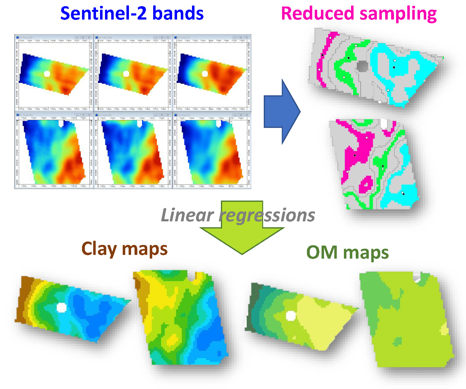
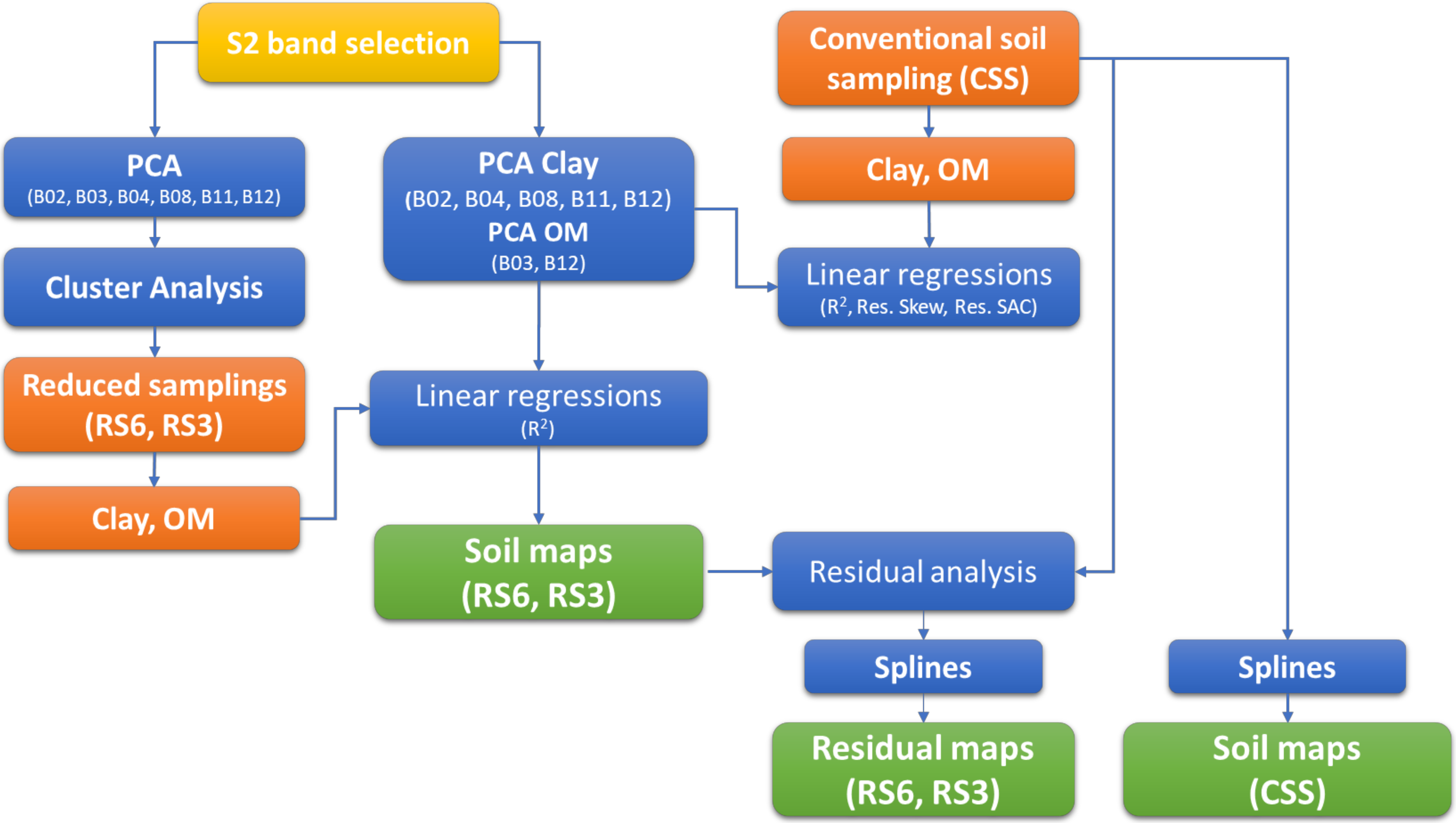
The general methodological workflow of the research is shown in Figure 1. After a preliminary S2 band selection based on the available bibliography, a Principal Components Analysis (PCA) was performed to reduce multicollinearity between all selected S2 bands. A subsequent cluster analysis was aimed to identify the sampling points for two reduced sampling schemes. The data from samples collected according to the reduced scheme were used in linear regressions with PCs of selected clay and OM bands to produce maps for the soil parameters under investigation. The reliability of these maps was assessed by comparing them with the analytical data acquired with a conventional soil sampling (CSS). An additional linear regression between the first Principal Components (PCs) and the clay and OM data obtained from the CSS was developed to understand and assess the relationships between the selected S2 bands and the soil properties of the fields under investigation.
2.1. Study Area
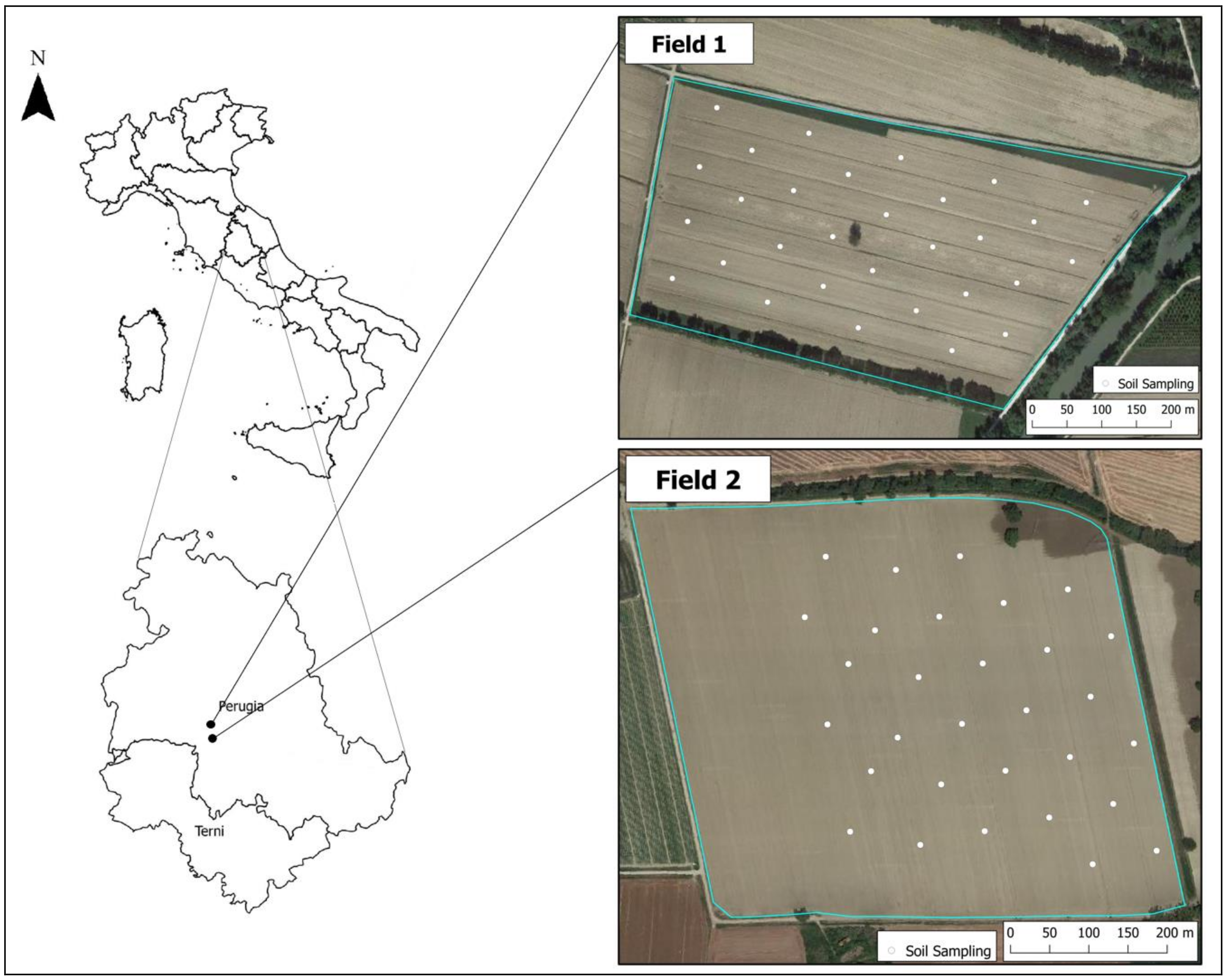
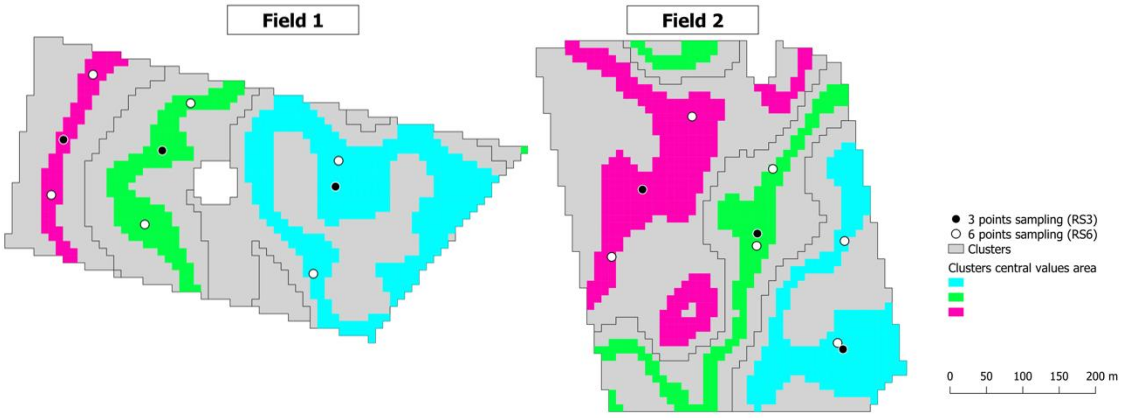
The experiments were carried out in two different plain fields, each about 20 ha wide, owned by the FIA, “Fondazione per l’Istruzione Agraria,” located in Tiber valley, near Deruta, Umbria, Italy (Figure 2). The study area is characterized by a Mediterranean climate, with a dry season from May to September and a cold and rainy season from October–November to March–April. According to the USDA soil taxonomy [30], the soils of the area, derived from fluvial and lacustrine sediments, are classified as Fluventic Haplustept. The study areas have no topographic gradient and are characterized by a soil textural gradient mainly related to their proximity to the Tiber stream at the east of both fields. Field 1 shows a more regular gradient than Field 2, characterized by a more evident local variability.
2.2. Identification of the Sampling Locations
All level 2A Sentinel-2 images with no cloud cover, timed close to the soil-sampling dates, were collected for the two study areas. The images, georeferenced according to WGS84-UTM32, were downloaded from The Copernicus Open-Access Hub. They were visually analyzed in false colors and compared, calculating the average NDVI to identify the most representative dates on which the two fields had the lowest vegetation percentage. Finally, the images of 28 September 2018 (Field 1) and 20 November 2019 (Field 2) were selected for the subsequent analysis.
Considering the scientific evidence reported in Table 1, we selected the S2 bands according to the evidence pointed out by Nanni and Demattê [17] for Landsat TM since they appeared the most adaptable to our case studies. In this vein, S2 bands included in the analysis were B02, B04, B08, B11, and B12 for clay and B03 and B12 for OM. A bilinear resampling to 10 meters was performed in SAGA GIS (version 7.5.0) [31] on the two S2 20-m resolution bands (B11, B12) to uniform the bands’ spatial resolution.
A K-means cluster analysis was carried out in SAGA GIS to identify natural groupings in the data and spatially identify the reduced soil-sample schemes’ optimal configuration for each field. To this aim, in the same software, a Principal Component Analysis (PCA) based on the variance-covariance matrix method was performed for each field to reduce the multicollinearity between input bands. In this step, all S2 selected bands (B02, B03, B04, B08, B11, and B12) were included for each field. The optimal number of clusters was found following the elbow method by analyzing the average cluster variance obtained by increasing their number [32,33,34]. The cluster’s center value +/– 2% was used to identify the most representative area of the cluster spatially. The final sampling location was defined manually, trying to locate two samples per cluster spaced apart within the said area or only one sample in the central part of the same area. Thus, two reduced soil-sampling schemes were defined for each field using two or one samples per cluster.
2.3. Soil Sampling
For comparison purposes, besides the said reduced sampling schemes, a conventional soil sampling (CSS) composed of 30 samples for each field was performed according to a regular georeferenced grid (Figure 2). Soil sampling was performed on 14 November 2018 for Field 1 and 17 December 2019 for Field 2. Each sample was composed of 3 bulks collected by an auger (0–40 cm) at about 5 meters from the reference sampling location. The samples were dried for three days in the oven at 30 °C and used for the physical–chemical analyses. After that, the samples were ground and passed through a 2-mm sieve after drying. Specifically, the soil samples were analyzed for their texture by the pipette method [35] and organic matter (OM) content by Walkley–Black method [36]. Using the USDA methodology, a textural characterization was performed on all soil samples from both fields [37]. Boxplots for clay and OM were plotted to compare data distributions of the three sampling schemes.
2.4. Linear Regression Analysis
Before proceeding to linear regression analysis, a PCA for each field and soil parameter was carried out in SAGA GIS, including the selected S2 bands. Only the first PC for all the four combinations was included in the subsequent regression steps, considering the very high explained cumulative variance of such components.
The output of the two reduced soil-sampling schemes was modeled through a Linear Regression Analysis (LRA), including the first PC for OM and clay contents, to assess their relationships and calculate linear equations applicable for generating maps of these two parameters. An additional LRA was performed between the first PCs and the CSS outputs to compare and assess the relationships between the S2 bands and clay and OM and possibly confirm the evidence reported in the bibliography. In this case, PCs were sampled by calculating the average value within a 20-m radius from the soil-sampling points using the “raster statistics for polygons” tool of SAGA GIS. A supplementary analysis was developed in R software to verify the base assumptions of LRA (heteroscedasticity, normal distribution of residuals, and Moran’s spatial autocorrelation of residuals).
All inferential statistical analysis, LRA, R2, and residual analysis were performed using the statistics software R [38] (Version 4.0.3) with the “agricolae” [39] (Version 1.3.3) and “DHARMa” (Version 0.3.3.0) [40] packages. The inferential statistical analysis in this study was conducted separately for the two fields, considering them as independent experiments.
To assess the reliability of clay and OM maps derived from the LRA of reduced sampling schemes, they were compared with the CSS visually and quantitatively through a residual analysis. In the former, maps produced using only a few samples and predictors from S2 and a map generated with conventional sampling and mapping methods (splines) are visually compared. For the latter, clay and OM maps derived from the reduced sampling schemes were sampled by calculating the average value within a 20-m radius from the soil-sample points of the conventional scheme. In this step, the “raster statistics for polygons” tool of SAGA GIS was used. The residuals calculated for clay and OM in this step were also spatialized in SAGA GIS using the spline method to understand their variability across the fields. In this step, the “Multilevel b-spline interpolation” tool was used.
3. Results
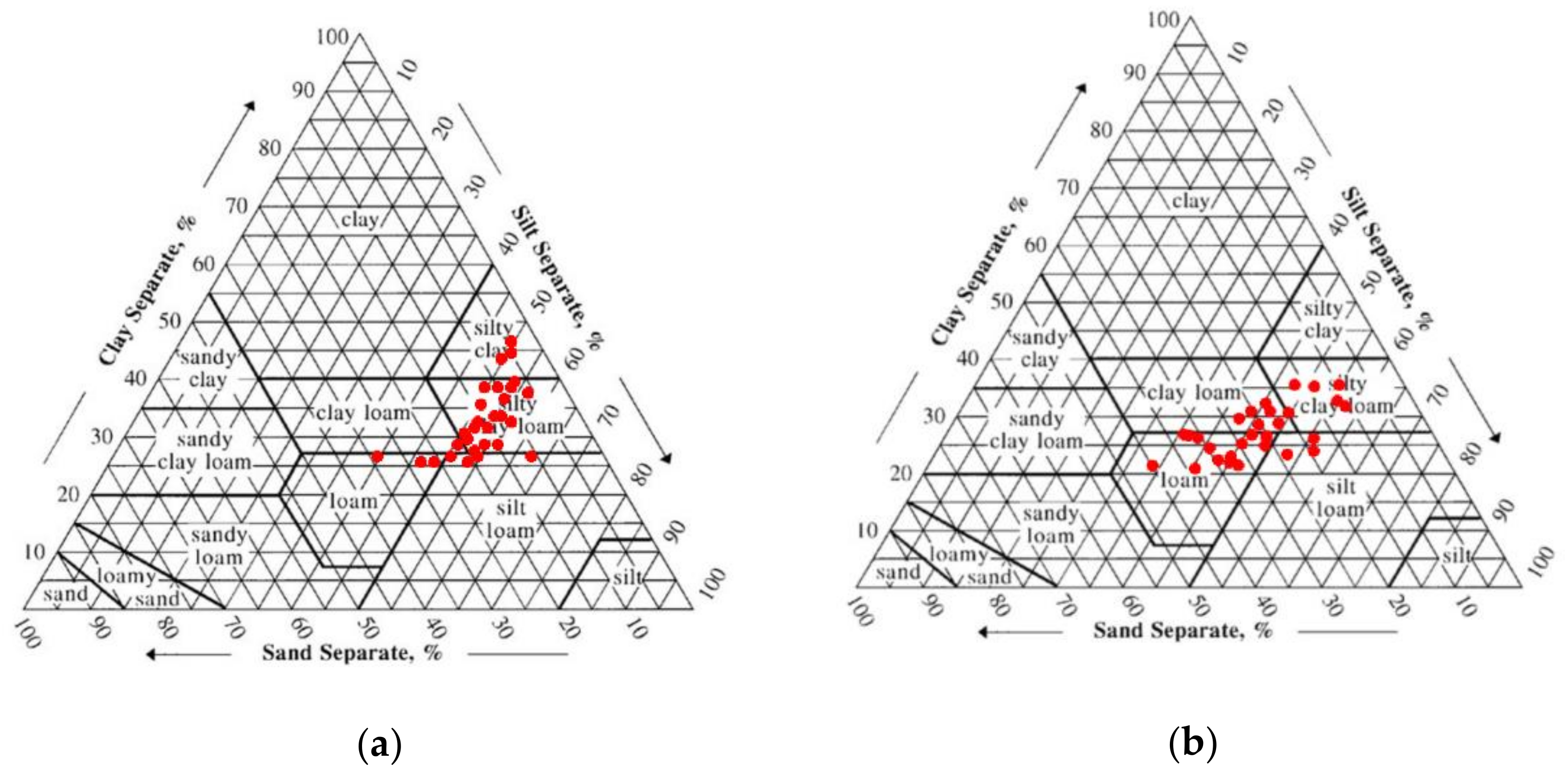
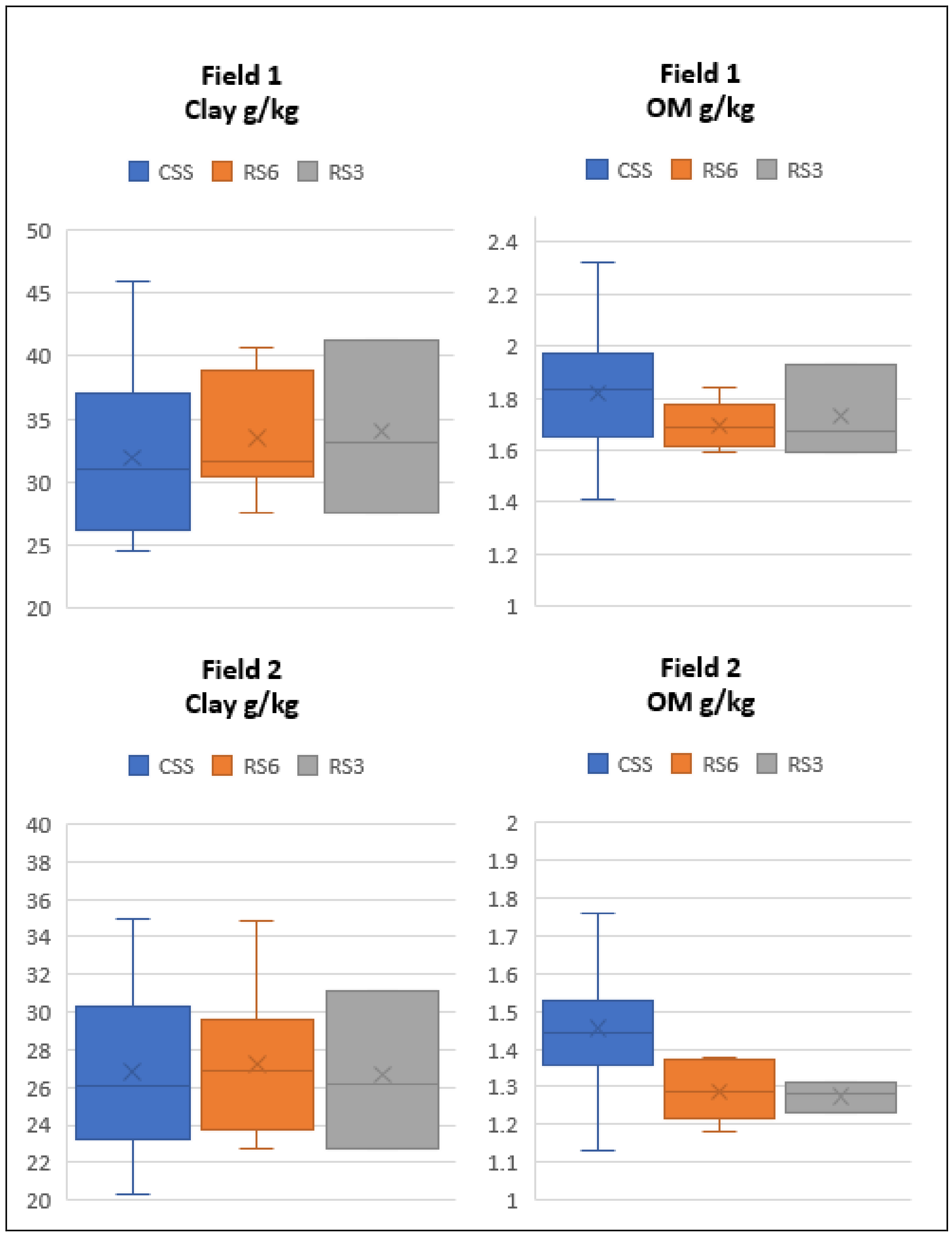
According to the USDA soil textural classification [37], the samples collected in Field 1 fall mainly in the silty-clay-loam texture class, whereas those collected in Field 2 are distributed in three different textural classes: loam, clay-loam, and silty-clay-loam (Figure 3). Regarding the clay content, for Field 1, we found a minimum value of 24.6% and a maximum of 46%, with a range of 21.4%. For Field 2, we found a minimum of 20.3% and a maximum of 35%, with a range of 14.7%. The OM content showed a minimum value of 1.41% and a maximum of 2.32% with a range of 0.91% for Field 1 and a minimum of 1.10% and a maximum of 2.19% with a range of 1.09% for Field 2. The boxplots of clay and Organic matter (OM) data from the three sampling methods show how the reduced sampling schemes capture the actual soil variability in the two fields (Figure 4).
Three clusters were identified using the elbow method for both fields as the optimal number of clusters. The central areas of these clusters were used to locate the soil samples of the reduced sampling schemes, which, considering the number of clusters, was composed of six (RS6) and three samples (RS3) for each field (Figure 5).
PCA results of the selected S2 bands (B02, B03, B04, B08, B11, and B12) for both fields and soil parameters are reported in Table 2 (clay content) and Table 3 (OM content). The first PCs, in all cases, account for the vast majority of the information contained in the S2 bands (some representative S2 bands are shown in Figure S1).
Outputs of LRAs, including the first PCs and reduced schemes samples (RS6 and RS3), are shown in Table 4. R-squared values for clay indicate for Field 1, and both RS6 and RS3 indicate a good fitting of the linear models (R2 for RS6: 0.88**, R2 for RS3: 0.99**). In the same field, the models of OM show a medium-high correlation of the predictor using RS6 (0.74**), whereas for RS3, even though it shows a higher correlation (0.96), it results are less significant. For Field 2, the linear models were less effective for clay and OM both for RS6 and RS3. Only for clay and RS6 does the model shows a medium correlation (R2 = 0.67*).
LRA outputs for the CSS are shown in Table 5. R-squared values indicate for Field 1 a high correlation of the predictors with clay content (0.85) and a medium-high correlation with OM content (0.65). Medium-low correlations were found in Field 2 both for clay (0.31) and OM (0.32) contents. The tests on the residuals highlighted only a partial skewness for OM in Field 2 and a slight spatial autocorrelation for clay in Field 1.
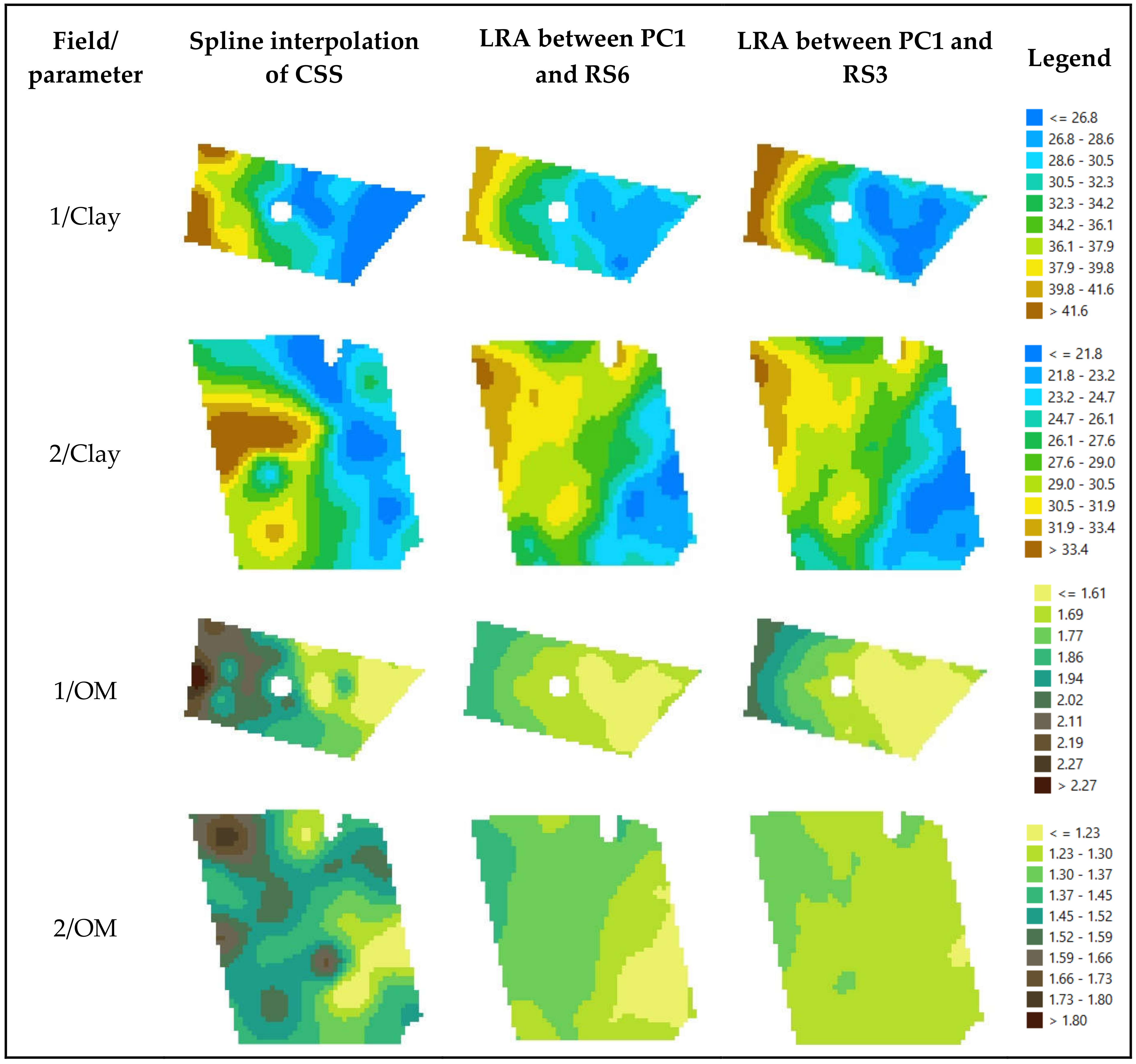
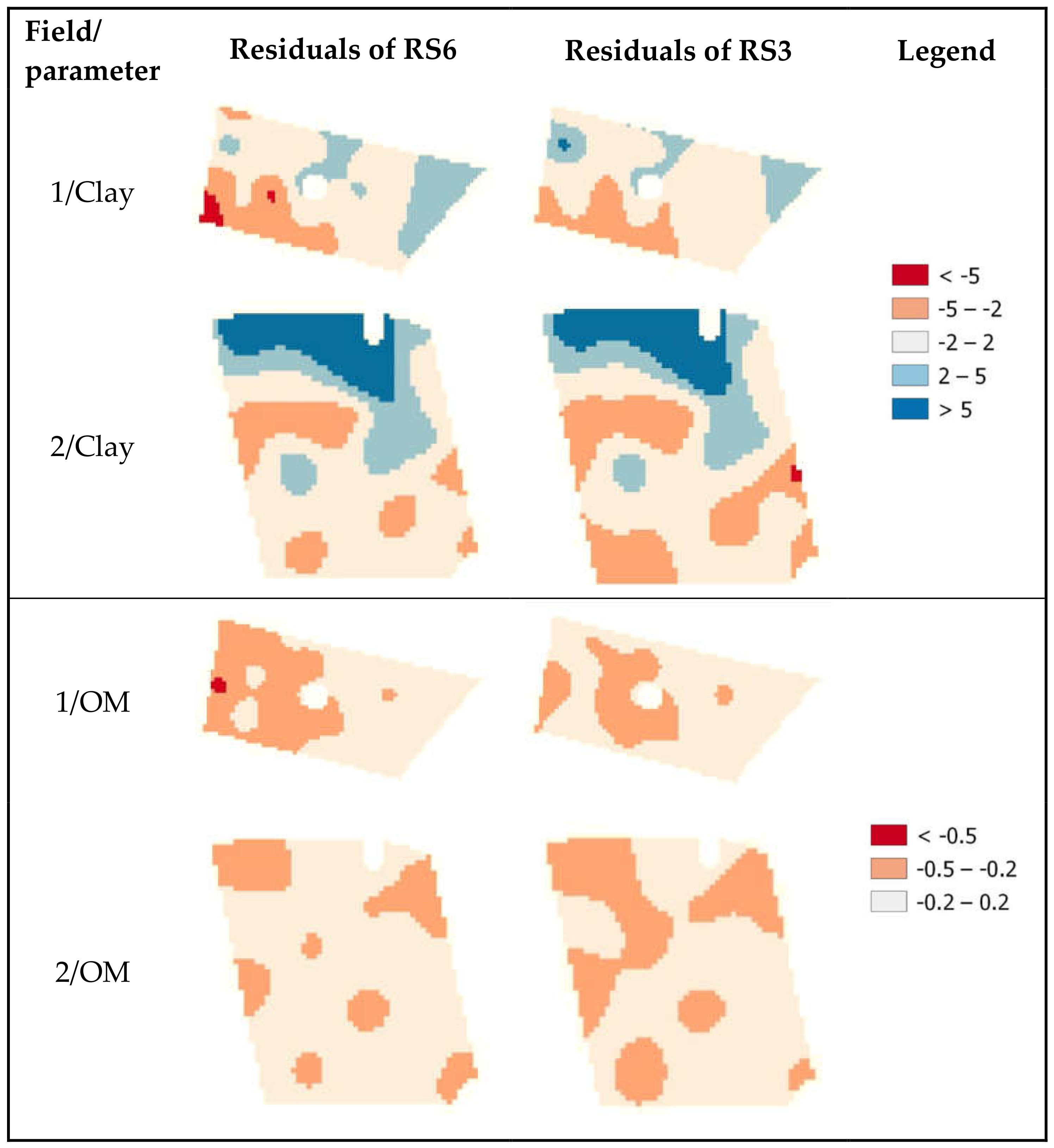
Clay and OM maps from LRA on RS6 and RS3 were visually compared with the map obtained from CSS using spline interpolation (Figure 6). Correlation and statistics of residuals between RS6 and RS3 maps and the correspondent, measured CSS values support a quantitative assessment of results (Table 6). The distribution of residuals is shown in the Supplementary Material (Figure S2 and Figure S3). Maps of these residuals obtained using spline interpolation show the spatial variability of the residuals (Figure 7).
4. Discussion
Our study investigated a methodology for quantitative characterization of clay and OM at the field scale based on remotely sensed data by Sentinel 2 and reduced soil sampling. Our results confirmed the evidence widely reported in the literature on a regional scale about the ability of optical remote sensing to support the soil texture and OM gradients estimation. We obtained comparable results of previous studies, highlighting a correlation between the visible and infrared bands with the soil OM content [16,17,19,23,24,25]. At the same time, results obtained for clay confirmed the evidence reported in previous relevant studies [16,17,27].
The proposed methodology is low cost and mainly based on unsupervised classification of RS data. Compared to other cited approaches to optimize soil sampling [2,5,28,29], it is more straightforward and easy to implement even within modern, web-based decision-support systems supporting precision agriculture [13]. The unsupervised classification of S2 data, based on K-means cluster analysis, represents a key methodological step. In this regard, we applied the widely used Elbow method to identify the optimal cluster number. Other approaches, possibly more effective in detecting representative spatial clusters, could be applied and tested in this step (e.g., average silhouette [41], gap statistic [42]). Moreover, other more advanced clustering methods, able to consider spatial relationships among pixels, even object based and including textural information with higher resolution images [43,44], could be tested for this purpose.
The correlations of linear models were considerably more significant in Field 1 than in Field 2 (Table 4). The high R2 values highlighted an encouraging performance of RS techniques in identifying the general gradient of the field. Indeed, R2 values were higher in the regression with the conventional sampling scheme since there was no detection of the local variability of the gradient in the reduced sampling. On the other hand, the small number of samples decreased the significance level (p-value). The method’s validity lay in the basic assumption that the predictors used were significantly related to the respective soil parameters, as demonstrated in the conventional sampling-scheme regression (Table 5) and reported in the literature.
The soil sampling highlighted a regular increasing clay and OM content trend in the former, moving from west to east. Differently, for the latter, the sampling showed a more irregular gradient both for the OM and for clay contents, with a spatial trend characterized by local variations of these parameters but with a visible base gradient given by increasing quantities of clay moving from east to west and increasing quantities of OM from southeast to northwest. The more significant local variability occurring for Field 2 than for Field 1 was attributed to its topographic position. Indeed, Field 2 is located very close to the Tiber river, and it is conceivable that the fluvial dynamics over time have influenced the characteristics of the soil, particularly its texture. This fact may explain the low correlation with remote sensing data, which were able to identify only the primary spatial trend (Figure 6) of the soil gradient, losing the information linked to local variations. However, concerning Field 1, despite the high correlation between clay content and the relative PC, the latter did not explain the whole variability across the field, as highlighted by the slight spatial autocorrelation between the residuals (Moran’s I Test < 0.05) (Table 5). In the case of Field 2, on the other hand, although the absence of spatial autocorrelation between the residuals (Moran’s I Test > 0.05) (Table 5), the low correlation between the soil parameters and the respective PCs suggested the presence of a good portion of variability not explained by the predictors.
As reported by the textural analysis (Figure 3), the samples are placed in a narrow range of the USDA textural triangle for both fields. Most of the samples from Field 1 are placed within the silty-clay-loam textural class, whereas the samples from Field 2 are mainly distributed in three classes (loam, clay loam, and silty-clay-loam). The analysis of textural classes and the soil parameters’ variation range showed that the gradient, although existing, was not so marked in Field 2, partly explaining the difficulty of remote sensing to identify it. This evidence is confirmed by boxplots of data from the different sampling methods (Figure 4). The reduced sampling schemes captured most of the variability of clay in both fields and of OM in Field 1 (RS3 performed better than RS6 in this case); differently, in Field 2, the reduced samplings did not express the (lower) variability of OM correctly.
For Field 1, the clay and OM maps, deriving from the reduced sampling, provided visually similar results compared with those obtained with the spline interpolation of the conventional sampling (Figure 6). The textural and OM gradients, increasing from east to west, are well represented in these maps. Figure 7 shows spatially the differences between the maps derived from the reduced samplings and remote sensing information and the maps derived from conventional sampling. In this regard, maps of Field 1 showed only slight differences, with most of the area characterized by differences of +/−2 % for clay (+/−5% maximum) and +/−0.2 % for OM (+/− 0.5% maximum). For Field 2, the differences were more marked, especially for the clay content, with peaks of more than −5% difference in the northern part of the field. The maps also showed the difficulty of remote sensing identifying the sharp, local variations characterizing the second field, with the maps taking on a “patchy” appearance.
As shown in Table 6, even using only three samples provided helpful information with results comparable to the six-point sampling. Compared to the conventional sampling, the normalized average error obtained from the RS3 maps is between 1.70% and 2.72% for clay and between 0.16% and 0.17% of OM. Moreover, for Field 1, almost 90% of the area of the RS3 maps show an estimation error between -3.50% and +3.36% for clay and between −0.32% and +0.08% for OM. For Field 2, the RS3 maps show a higher error, but they appear still usable for agronomic purposes, with 50% of the area characterized by an error between −2.09% and 2.86% for clay -0.22% and -0.11% for the OM.
5. Conclusions
Soil is one of the most significant factors for crop growth and yield, and its knowledge provides benefits for farm management. Soil-map making generally requires a very dense field sampling or more advanced and relatively expensive techniques. This research generally confirmed the state-of-the-art evidence of soil parameters detection by optical remote sensing. Moreover, the results demonstrated how remote sensing, even if approximately, can identify the general gradient trend of soil properties, such as clay and OM contents, in agricultural fields. Even though other additional experiments are necessary, results suggest that, using the proposed procedure based on Sentinel 2 data, it is possible to define a reduced sampling scheme useful for speeding-up on-field soil sampling operations. S2 data may help characterize a given soil gradient even using a few soil samples and differentiate the crops’ operations within a precision agriculture process.
Supplementary Materials
The following are available online at https://0-www-mdpi-com.brum.beds.ac.uk/article/10.3390/rs13173379/s1, Figure S1: Representative Sentinel 2 bands for the two fields under investigation; Figure S2: Distribution of residuals calculated for Field 1 (OM: Organic Matter, RS6: six samples, RS3: three samples); Figure S3: Distribution of residuals calculated for Field 2 (OM: Organic Matter, RS6: six samples, RS3: three samples).
Author Contributions
Conceptualization, F.S.S. and M.V.; methodology F.S.S., M.V., A.A. and A.L.; investigation, F.S.S.; data curation, F.S.S. and A.L.; writing—original draft preparation, F.S.S. and M.V.; writing—review and editing, M.V., F.S.S., A.A. and A.L.; visualization, F.S.S.; supervision, M.V. and A.A.; project administration, M.V.; All authors have read and agreed to the published version of the manuscript.
Funding
This research was developed within the framework of the project “RTK 2.0—Prototipizzazione di una rete RTK e di applicazioni tecnologiche innovative per l’automazione dei processi colturali e la gestione delle informazioni per l’agricoltura di precisione”—RDP 2014–2020 of Umbria—Meas. 16.1—App. 84250020256.
Institutional Review Board Statement
Not applicable.
Informed Consent Statement
Not applicable.
Data Availability Statement
Data are available, upon any reasonable request, from the authors.
Acknowledgments
The authors wish to thank Mauro Brunetti of the “Fondazione per l’Istruzione Agraria” farm and Daniele Luchetti of the FIELDLAB of the Department of Agricultural, Food, and Environmental Sciences, University of Perugia, for their constructive and valuable support during the experimental stages of the research.
Conflicts of Interest
The authors declare no conflict of interest.
References
- Flanders, D.; Hall-Beyer, M.; Pereverzoff, J. Preliminary evaluation of eCognition object-based software for cut block delineation and feature extraction. Can. J. Remote Sens. 2003, 29, 441–452. [Google Scholar] [CrossRef]
- Kerry, R.; Oliver, M.A.; Frogbrook, Z.L. Geostatistical Applications for Precision Agriculture; Springer: Dordrecht, The Netherlands, 2010; pp. 35–63. [Google Scholar] [CrossRef]
- Vizzari, M.; Santaga, F.; Benincasa, P. Sentinel 2-Based Nitrogen VRT Fertilization in Wheat: Comparison between Traditional and Simple Precision Practices. Agronomy 2019, 9, 278. [Google Scholar] [CrossRef] [Green Version]
- Messina, G.; Peña, J.M.; Vizzari, M.; Modica, G. A Comparison of UAV and Satellites Multispectral Imagery in Monitoring Onion Crop. An Application in the ‘Cipolla Rossa di Tropea’ (Italy). Remote Sens. 2020, 12, 3424. [Google Scholar] [CrossRef]
- Yuzugullu, O.; Lorenz, F.; Fröhlich, P.; Liebisch, F. Understanding Fields by Remote Sensing: Soil Zoning and Property Mapping. Remote Sens. 2020, 12, 1116. [Google Scholar] [CrossRef] [Green Version]
- Clay, D.E.; Carlson, C.G. Precision Soil Sampling. In iGrow Corn: Best Management Practices; Clay, D.E., Carlson, C.G., Clay, S.A., Byamukama, E., Eds.; South Dakota State University: Brookings, SD, USA, 2016. [Google Scholar]
- Wollenhaupt, N.C.; Wolkowski, R.P. Grid Soil Sampling. Better Crop. 1994, 78, 6–8. [Google Scholar]
- Corwin, D.L.; Lesch, S.M.; Oster, J.D.; Kaffka, S.R. Monitoring management-induced spatio-temporal changes in soil quality through soil sampling directed by apparent electrical conductivity. Geoderma 2006, 131, 369–387. [Google Scholar] [CrossRef]
- Messina, G.; Praticò, S.; Badagliacca, G.; Di Fazio, S.; Monti, M.; Modica, G. Monitoring Onion Crop “Cipolla Rossa di Tropea Calabria IGP” Growth and Yield Response to Varying Nitrogen Fertilizer Application Rates Using UAV Imagery. Drones 2021, 5, 61. [Google Scholar] [CrossRef]
- Oza, S.R.; Panigrahy, S.; Parihar, J.S. Concurrent use of active and passive microwave remote sensing data for monitoring of rice crop. Int. J. Appl. Earth Obs. Geoinf. 2008, 10, 296–304. [Google Scholar] [CrossRef]
- Zheng, Q.; Huang, W.; Cui, X.; Shi, Y.; Liu, L. New Spectral Index for Detecting Wheat Yellow Rust Using Sentinel-2 Multispectral Imagery. Sensors 2018, 18, 868. [Google Scholar] [CrossRef] [Green Version]
- Louis, J.; Debaecker, V.; Pflug, B.; Main-Knorn, M.; Bieniarz, J.; Mueller-Wilm, U.; Cadau, E.; Gascon, F. Sentinel-2 SEN2COR: L2A Processor for Users, Proceedings of the Living Planet Symposium 2016, Prague, Czech Republic, 9–13 May 2016; European Space Agency: Paris, France, 2016; pp. 1–8. [Google Scholar]
- Santaga, F.S.; Benincasa, P.; Toscano, P.; Antognelli, S.; Ranieri, E.; Vizzari, M. Simplified and Advanced Sentinel-2-Based Precision Nitrogen Management of Wheat. Agronomy 2021, 11, 1156. [Google Scholar] [CrossRef]
- Ben-Dor, E.; Banin, A. Near-Infrared Analysis as a Rapid Method to Simultaneously Evaluate Several Soil Properties 94. Soil Sci. Soc. Am. J. 1995, 59, 364–372. [Google Scholar] [CrossRef]
- Ge, Y.; Thomasson, J.A.; Sui, R. Remote Sensing of Soil Properties in Precision Agriculture: A Review. Front. Earth Sci. 2011, 5, 229–238. [Google Scholar] [CrossRef]
- Ahmed, Z.; Iqbal, J. Evaluation of Landsat TM5 multispectral data for automated mapping of surface soil texture and organic matter in GIS. Eur. J. Remote Sens. 2014, 47, 557–573. [Google Scholar] [CrossRef] [Green Version]
- Nanni, M.R.; Demattê, J.A.M. Spectral Reflectance Methodology in Comparison to Traditional Soil Analysis. Soil Sci. Soc. Am. J. 2006, 70, 393. [Google Scholar] [CrossRef]
- Gholizadeh, A.; Daniel, Ž.; Saberioon, M. Remote Sensing of Environment Soil organic carbon and texture retrieving and mapping using proximal, airborne and Sentinel-2 spectral imaging. Remote Sens. Environ. 2018, 218, 89–103. [Google Scholar] [CrossRef]
- Daniel, K.W.; Tripathi, N.K.; Honda, K.; Apisit, E. Analysis of vnir (400–1100nm) spectral signatures for estimation of soil organic matter in tropical soils of thailand. Int. J. Remote Sens. 2004, 25, 83–91. [Google Scholar] [CrossRef]
- Hummel, J.W.; Sudduth, K.A.; Hollinger, S.E. Soil moisture and organic matter prediction of surface and subsurface soils using an NIR soil sensor. Comput. Electron. Agric. 2001, 32, 149–165. [Google Scholar] [CrossRef]
- Masserschmidt, I.; Cuelbas, C.J.; Poppi, R.J.; De Andrade, J.C.; De Abreu, C.A.; Davanzo, C.U. Determination of organic matter in soils by FTIR/diffuse reflectance and multivariate calibration. J. Chemom. 1999, 13, 265–273. [Google Scholar] [CrossRef]
- McCarty, G.W.; Reeves, J.B. Comparison of near infrared and mid infrared diffuse reflectance spectroscopy for field-scale measurement of soil fertility parameters. Soil Sci. 2006, 171, 94–102. [Google Scholar] [CrossRef] [Green Version]
- Palacios-Orueta, A.; Ustin, S.L. Remote sensing of soil properties in the Santa Monica Mountains I. Spectral analysis. Remote Sens. Environ. 1998, 65, 170–183. [Google Scholar] [CrossRef]
- Shibusawa, S.; Anom, S.W.; Sato, S.; Sasao, A.; Hirako, S. Soil mapping using the realtime soil spectrophotometer. Precis. Agric. 2001, 1, 497–508. [Google Scholar]
- Stamatiadis, S.; Christofides, C.; Tsadilas, C.; Samaras, V.; Schepers, J.S.; Francis, D. Ground-sensor soil reflectance as related to soil properties and crop response in a cotton field. Precis. Agric. 2005, 6, 399–411. [Google Scholar] [CrossRef]
- Xue, J.; Su, B. Significant remote sensing vegetation indices: A review of developments and applications. J. Sens. 2017, 2017. [Google Scholar] [CrossRef] [Green Version]
- Barnes, E.M.; Baker, M.G. Multispectral data for mapping soil texture: Possibilities and limitations. Appl. Eng. Agric. 2000, 16, 731–741. [Google Scholar] [CrossRef]
- Wang, Y.; Jiang, L.; Qi, Q.; Liu, Y.; Wang, J. Remote Sensing-Guided Sampling Design with Both Good Spatial Coverage and Feature Space Coverage for Accurate Farm Field-Level Soil Mapping. Remote Sens. 2019, 11, 1946. [Google Scholar] [CrossRef] [Green Version]
- Castaldi, F.; Chabrillat, S.; Wesemael, B. van Sampling Strategies for Soil Property Mapping Using Multispectral Sentinel-2 and Hyperspectral EnMAP Satellite Data. Remote Sens. 2019, 11, 309. [Google Scholar] [CrossRef] [Green Version]
- Soil Survey Staff. Keys to Soil Taxonomy, 12th ed.; USDA-Natural Resources Conservation Service: Washington, DC, USA, 2014.
- Conrad, O.; Bechtel, B.; Bock, M.; Dietrich, H.; Fischer, E.; Gerlitz, L.; Wehberg, J.; Wichmann, V.; Böhner, J. System for Automated Geoscientific Analyses (SAGA) v. 2.1.4. Geosci. Model Dev. 2015, 8, 1991–2007. [Google Scholar] [CrossRef] [Green Version]
- Kodinariya, T.M.; Makwana, P.R. Review on determining number of Cluster in K-Means Clustering. Int. J. Adv. Res. Comput. Sci. Manag. Stud. 2013, 1, 2321–7782. [Google Scholar]
- Purnima, B.; Arvind, K. EBK-Means: A Clustering Technique based on Elbow Method and K-Means in WSN. Int. J. Comput. Appl. 2014, 105, 17–24. [Google Scholar]
- Liu, F.; Deng, Y. Determine the number of unknown targets in Open World based on Elbow method. IEEE Trans. Fuzzy Syst. 2020, 6706, 1. [Google Scholar] [CrossRef]
- Day, P.R. Particle Fractionation and Particle-Size Analysis. In Methods of Soil Analysis, Part 1: Physical and Mineralogical Properties, Including Statistics of Measurement and Sampling; Black, C.A., Ed.; American Society of Agronomy: Madison, WI, USA, 1965; pp. 545–567. ISBN 9780891182030. [Google Scholar]
- Soltner, D. Le Bases de la Production Vegetale, 16th ed.; Tecniques, Collection Sciences et Agricoles: Angers, France, 1988. [Google Scholar]
- United States Department of Agriculture; Natural Resources Conservation Service. Soil Taxonomy: A Basic System of Soil Classification for Making and Interpreting Soil Surveys; US Department of Agriculture: Washington, DC, USA, 1975.
- RC Team. R: A Language and Environment for Statistical Computing; R Foundation for Statistical Computing: Vienna, Austria, 2016; Volume 2, pp. 1–12. ISBN 3-900051-070. [Google Scholar]
- De Mendiburu, F. Statistical Procedures for Agricultural Research. Package ‘Agricolae’; Comprehensive R Archive Network; Institute for Statistics and Mathematics: Vienna, Austria, 2013; Available online: http://cran.r-project.org/web/packages/agricolae/agricolae.pdf (accessed on 23 August 2017).
- Hartig, F. Package ‘DHARMa’. 2018. Available online: http://florianhartig.github.io/DHARMa/ (accessed on 10 July 2017).
- Rousseeuw, P.J. Silhouettes: A graphical aid to the interpretation and validation of cluster analysis. J. Comput. Appl. Math. 1987, 20. [Google Scholar] [CrossRef] [Green Version]
- Tibshirani, R.; Walther, G.; Hastie, T. Estimating the number of clusters in a data set via the gap statistic. J. R. Stat. Soc. Ser. B Stat. Methodol. 2001, 63. [Google Scholar] [CrossRef]
- Tassi, A.; Vizzari, M. Object-Oriented LULC Classification in Google Earth Engine Combining SNIC, GLCM, and Machine Learning Algorithms. Remote Sens. 2020, 12, 3776. [Google Scholar] [CrossRef]
- Blaschke, T.; Lang, S.; Lorup, E.; Strobl, J.; Zeil, P. Object-oriented image processing in an integrated GIS/remote sensing environment and perspectives for environmental applications. Environ. Inf. Plan. Politics Public 2000, 2, 555–570. [Google Scholar]
Figure 1.
Methodological workflow of the research.

Figure 2.
The geographical location of the study areas and sample locations of the conventional soil-sampling (CSS) scheme.
Figure 2.
The geographical location of the study areas and sample locations of the conventional soil-sampling (CSS) scheme.

Figure 3.
Soil texture distributions of the samples collected in Field 1 (a) and Field 2 (b).

Figure 4.
Boxplots of clay and organic matter (OM) data from the three sampling methods (CSS: Conventional Soil Sampling; RS6: six samples; RS3: three samples).
Figure 4.
Boxplots of clay and organic matter (OM) data from the three sampling methods (CSS: Conventional Soil Sampling; RS6: six samples; RS3: three samples).

Figure 5.
Cluster, central values areas, and reduced soil-sampling schemes composed of three samples (black points) and six samples (white points) for Field 1 and 2.
Figure 5.
Cluster, central values areas, and reduced soil-sampling schemes composed of three samples (black points) and six samples (white points) for Field 1 and 2.

Figure 6.
Comparison between maps obtained from spline interpolation of the measured clay and OM values of CSS (Conventional Sampling Scheme) and LRA of the two reduced sampling schemes (RS6: six samples, RS3: three samples).
Figure 6.
Comparison between maps obtained from spline interpolation of the measured clay and OM values of CSS (Conventional Sampling Scheme) and LRA of the two reduced sampling schemes (RS6: six samples, RS3: three samples).

Figure 7.
Maps obtained from spline interpolation of the residuals calculated between Clay and OM maps from the two reduced sampling schemes (RS6: six samples, RS3: three samples) and measured CSS values (Conventional Sampling Scheme).
Figure 7.
Maps obtained from spline interpolation of the residuals calculated between Clay and OM maps from the two reduced sampling schemes (RS6: six samples, RS3: three samples) and measured CSS values (Conventional Sampling Scheme).


Table 1.
Relationships between soil properties and satellite data found in literature. The OM section was developed starting from Ahmed & Iqbal [16].
Table 1.
Relationships between soil properties and satellite data found in literature. The OM section was developed starting from Ahmed & Iqbal [16].
| Soil Property | Satellite | Spectral Region, Index or Regression Formula | Spectral Range (nm) | R2 | Pearson Index | Reference |
|---|---|---|---|---|---|---|
| OM | Landsat TM | 2.24 − 0.021 × (TM1) − 0.0165 × (TM6) + 0.0087 × (TM7) | 0.54 | [16] | ||
| TM1 | 450–520 | −0.701 | ||||
| TM6 | 10,400–12,500 | −0.494 | ||||
| TM7 | 2080–2350 | −0.500 | ||||
| 7.084 − 0.109 (TM7) − 0.102 (TM2) | 0.51 | [17] | ||||
| Sentinel 2 | BI = √((red × red) + (green × green))/2 | [18] | ||||
| BI2 = √((red × red) + (green × green) + (nir × nir))/3 | ||||||
| GNDVI = (NIR-green)/(NIR + green) | ||||||
| B4 (red) | 665 | |||||
| B5 (red-edge) | 705 | |||||
| SATVI = ((B11- B4)/(B11 + B4 + 0.5)) × (1 + 0.5)-B12/2 | ||||||
| B11 | 1565–1655 | |||||
| B12 | 2100–2280 | |||||
| SPOT (Satellite Probatoire d’Observation de la Terre) | VIS–NIR | 400–1190 | 0.59 | [19] | ||
| NIR | 1603–2598 | 0.79 | [20] | |||
| MIR | 2500–25,000 | 0.98 | [21] | |||
| NIR | 1000–2500 | 0.92 | [22] | |||
| UV–VIS–NIR | 200–2500 | 0.53 | [23] | |||
| VIS–NIR | 400–2400 | 0.65 | [24] | |||
| VIS | 400–680 | 0.68 | [25] | |||
| MSAVI2 = (2 × nir+1-√((2 × nir+1)2 − 8 × (nir-red)))/2 | [26] | |||||
| CLAY | Landsat TM | TM4 (nir) | 760–900 | 0.709 | [16] | |
| −5.24 + 1.35 × (TM4) − 0.32 × (TM6) | 0.51 | |||||
| TM3 (red) | 630–690 | −0.473 | [27] | |||
| TM4 (nir) | 760–900 | −0.494 | ||||
| TM5 | 1550–1750 | −0.524 | ||||
| TM7 | 2080–2350 | −0.568 | ||||
| 27.03 − 1.260(TM1) + 0.363(TM3) − 0.301(TM4) + 0.305(TM5) − 0.848 (TM7) | 0.67 | [17] | ||||
| Sentinel 2 | MSAVI | [18] | ||||
| MSAVI2 = (2 × nir + 1 − √((2 × nir + 1)2 − 8 × (nir-red)))/2 | ||||||
| SAVI= ((1 + L) × (nir − red))/(nir + red + L) L = 0.5 | ||||||
| B7 (nir) | 783 | |||||
| V = nir/red | ||||||
| SAND | Landsat TM | TM3 (red) | 630–690 | 0.462 | [27] | |
| TM4 (nir) | 760–900 | 0.493 | ||||
| TM5 | 1550–1750 | 0.526 | ||||
| TM7 | 2080–2350 | 0.572 | ||||
| 13.54 + 0.934(TM1) − 0.228(TM5) + 0.663(TM7) | 0.52 | [17] | ||||
| SILT | Landsat TM | B4 (nir) | 760–900 | 0.714 | [16] | |
| 86.78 +1.26 × (TM4) − 1.91 × (TM6) | 0.72 | |||||
| TM6 | 10,400–12,500 | −0.571 | ||||
| TM3 (red) | 630–690 | −0.426 | [27] | |||
| TM4 (nir) | 760–900 | −0.466 | ||||
| TM5 | 1550–1750 | −0.502 | ||||
| TM7 | 2080–2350 | −0.547 |
Table 2.
Principal components (PC), cumulative variance, and contribution to each component from the selected S2 bands for clay.
Table 2.
Principal components (PC), cumulative variance, and contribution to each component from the selected S2 bands for clay.
| Field | PC | Cumulative Variance | B02 | B04 | B08 | B11 | B12 |
|---|---|---|---|---|---|---|---|
| 1 | 1 | 99.47 | 5% | 37% | 14% | 35% | 9% |
| 2 | 99.93 | 11% | 16% | 20% | 1% | 52% | |
| 3 | 99.94 | 14% | 18% | 5% | 42% | 20% | |
| 4 | 99.98 | 31% | 4% | 47% | 7% | 10% | |
| 5 | 100 | 39% | 25% | 14% | 14% | 9% | |
| 2 | 1 | 98.93 | 6% | 26% | 1% | 27% | 41% |
| 2 | 99.72 | 17% | 40% | 2% | 0% | 41% | |
| 3 | 99.9 | 22% | 7% | 51% | 14% | 5% | |
| 4 | 99.94 | 31% | 27% | 3% | 33% | 6% | |
| 5 | 100 | 24% | 0% | 43% | 26% | 7% |
Table 3.
Principal components (PC), cumulative variance, and contribution to each component from the selected S2 bands for OM (Organic Matter).
Table 3.
Principal components (PC), cumulative variance, and contribution to each component from the selected S2 bands for OM (Organic Matter).
| Field | PC | Cumulative Variance | B3 | B12 |
|---|---|---|---|---|
| 1 | 1 | 99.45 | 16% | 84% |
| 2 | 100 | 84% | 16% | |
| 2 | 1 | 99.43 | 31% | 69% |
| 2 | 100 | 69% | 31% |
Table 4.
Linear Regression Analysis outputs for reduced sampling schemes (RS6: six samples, RS3: three samples).
Table 4.
Linear Regression Analysis outputs for reduced sampling schemes (RS6: six samples, RS3: three samples).
| Attributes and Field | Sampling Scheme | Linear Regression Equation | R2 | p-Value | Residuals Standard Error | Residuals |
|---|---|---|---|---|---|---|
| Clay Field 1 | RS6 | 69.059722 + 0.006234 × clay_PC1 | 0.88 | <0.01 | 1.927 | −0.597; 1.672; −1.183; −1.494; −1.040; 2.642. |
| RS3 | 79.033123 + 0.007860 × clay_PC1 | 0.99 | <0.01 | 0.077 | 0.026; −0.063; −0.037. | |
| Clay Field 2 | RS6 | 61.553787 + 0.012154 × clay_PC1 | 0.67 | <0.05 | 2.719 | −0.338; 1.074; −1.505; −0.396; 4.132; −2.967. |
| RS3 | 62.591025 + 0.012745 × clay_PC1 | 0.96 | 0.13 | 1.197 | 0.396; −0.972; 0.576. | |
| OM Field 1 | RS6 | 2.287063 − 0.000165 × om_PC1 | 0.74 | < 0.05 | 0.055 | 0.049; −0.055; −0.051; 0.063; −0.017; 0.011. |
| RS3 | 2.783529 − 0.000292 × om_PC1 | 0.96 | 0.13 | 0.050 | 0.017; −0.041; 0.024. | |
| OM Field 2 | RS6 | 1.806841 − 0.000332 × om_PC1 | 0.49 | 0.12 | 0.063 | 0.008; −0.042; 0.015; 0.072; −0.087; 0.034. |
| RS3 | 1.504280 − 0.000148 × om_PC1 | 0.47 | 0.52 | 0.041 | −0.014; 0.034; −0.019. |
Table 5.
Output parameters from linear regressions between selected PCs and soil clay and OM of CSS (Conventional Sampling Scheme). * Significance at the p < 0.01 level of probability. ** p < 0.05 means the existence of spatial autocorrelation between the residuals.
Table 5.
Output parameters from linear regressions between selected PCs and soil clay and OM of CSS (Conventional Sampling Scheme). * Significance at the p < 0.01 level of probability. ** p < 0.05 means the existence of spatial autocorrelation between the residuals.
| Attributes | Field | Linear Regression Equation | R2 * | Residuals Skewness | Residuals Moran’s I Test (p-Value) ** |
|---|---|---|---|---|---|
| Clay | 1 | 80.02 + 0.00807 × clay_PC1 | 0.85 | 0.01 | <0.05 |
| 2 | 52.693993 + 0.009253 × clay_PC1 | 0.36 | −0.51 | >0.05 | |
| OM | 1 | 3.267 − 0.0003844 × om_PC1 | 0.65 | 0.01 | >0.05 |
| 2 | 2.278136 − 0.000554 × om_PC1 | 0.40 | 0.20 | >0.05 |
Table 6.
Statistics of residuals calculated between clay and OM maps from the two reduced sampling schemes (RS6: six samples, RS3: three samples) and measured values of CSS (Conventional Sampling Scheme).
Table 6.
Statistics of residuals calculated between clay and OM maps from the two reduced sampling schemes (RS6: six samples, RS3: three samples) and measured values of CSS (Conventional Sampling Scheme).
| Field 1 | Field 2 | |||||||
|---|---|---|---|---|---|---|---|---|
| Clay | Organic Matter | Clay | Organic Matter | |||||
| 6 samples | 3 samples | 6 samples | 3 samples | 6 samples | 3 samples | 6 samples | 3 samples | |
| Normalized average error | 1.95 | 1.70 | 0.19 | 0.16 | 2.65 | 2.72 | 0.14 | 0.17 |
| st.dev | 2.390 | 2.046 | 0.150 | 0.116 | 3.314 | 3.374 | 0.092 | 0.107 |
| average | −0.05 | 0.11 | −0.15 | −0.14 | 1.09 | 0.51 | −0.14 | −0.16 |
| min | −6.03 | −4.94 | −0.54 | −0.41 | −4.42 | −5.44 | −0.40 | −0.46 |
| max | 4.15 | 5.27 | 0.20 | 0.17 | 9.46 | 8.96 | 0.11 | 0.14 |
| RMSE | 2.66 | 2.35 | 0.23 | 0.19 | 3.70 | 3.67 | 0.18 | 0.20 |
Publisher’s Note: MDPI stays neutral with regard to jurisdictional claims in published maps and institutional affiliations. |
© 2021 by the authors. Licensee MDPI, Basel, Switzerland. This article is an open access article distributed under the terms and conditions of the Creative Commons Attribution (CC BY) license (https://creativecommons.org/licenses/by/4.0/).
Share and Cite
MDPI and ACS Style
Santaga, F.S.; Agnelli, A.; Leccese, A.; Vizzari, M. Using Sentinel-2 for Simplifying Soil Sampling and Mapping: Two Case Studies in Umbria, Italy. Remote Sens. 2021, 13, 3379. https://0-doi-org.brum.beds.ac.uk/10.3390/rs13173379
AMA Style
Santaga FS, Agnelli A, Leccese A, Vizzari M. Using Sentinel-2 for Simplifying Soil Sampling and Mapping: Two Case Studies in Umbria, Italy. Remote Sensing. 2021; 13(17):3379. https://0-doi-org.brum.beds.ac.uk/10.3390/rs13173379
Chicago/Turabian StyleSantaga, Francesco Saverio, Alberto Agnelli, Angelo Leccese, and Marco Vizzari. 2021. "Using Sentinel-2 for Simplifying Soil Sampling and Mapping: Two Case Studies in Umbria, Italy" Remote Sensing 13, no. 17: 3379. https://0-doi-org.brum.beds.ac.uk/10.3390/rs13173379
Note that from the first issue of 2016, this journal uses article numbers instead of page numbers. See further details here.