NaturaSat—A Software Tool for Identification, Monitoring and Evaluation of Habitats by Remote Sensing Techniques

Abstract

The NaturaSat software integrates various image processing techniques together with vegetation data, into one multipurpose tool that is designed for performing facilities for all requirements of habitat exploration, all in one place. It provides direct access to multispectral Sentinel-2 data provided by the European Space Agency. It supports using these data with various vegetation databases, in a user-friendly environment, for, e.g., vegetation scientists, fieldwork experts, and nature conservationists. The presented study introduces the NaturaSat software, describes new powerful tools, such as the semi-automatic and automatic segmentation methods, and natural numerical networks, together with validated examples comparing field surveys and software outputs. The software is robust enough for field work researchers and stakeholders to accurately extract target units’ borders, even on the habitat level. The deep learning algorithm, developed for habitat classification within the NaturaSat software, can also be used in various research tasks or in nature conservation practices, such as identifying ecosystem services and conservation value. The exact maps of the habitats obtained within the project can improve many further vegetation and landscape ecology studies.

1. Introduction

Remote sensing has become one of the essential methods used to effectively and directly acquire information on the Earth’s surface [1,2]. Together with standardized plots and regular in situ measurements, remote sensing is a powerful monitoring engine [3,4], playing an irreplaceable role in acquiring data and fulfilling its potential as an essential tool for evaluating and implementing environmental policy [1]. In a changing world, with increasing pressure on natural resources, land-cover maps and monitoring have reached substantial importance for area planning and resource management [5].

Competent planning and decision making in biodiversity and ecosystem conservation, restoration, and sustainable development are urgently needed. Remote sensing data and ecological models can play a crucial role in supporting this need and safeguarding natural assets [2]. The robustness and complexity of the obtained data in remote sensing indicate their multi-source, multi-scale, high-dimensional, and dynamic-state characteristics. The existing techniques and methods are limited to solve many problems that are a big data challenge, such as difficulty processing and analyzing data in a reasonable time, identifying the correct data to achieve the given task, finding a meaningful structure, etc. [6].

Remote sensing is one of the most important tools in ecology and conservation, for the effective monitoring of ecosystems in space and time [7]. Satellite remote sensing of ecosystem functions could offer many opportunities to advance ecology and conservation, including testing emerging theories and unveiling the processes shaping the impacts of anthropogenic threats on biodiversity more rapidly [8]. Using satellite images for monitoring habitats and biotic dynamics has been highlighted in various categories of research activities. There is enormous potential, due to the recent developments of various technologies (either hardware or software). Since the maintenance of biodiversity, based on conserving semi-natural and natural habitats, is one of the targets of the European 2020 Biodiversity Strategy [3], developing reliable methods and tools, substituting time-consuming expert knowledge and field work, is urgent. There are, of course, many challenges in such methodologies, including mapping ecotone transitions between vegetation types or the low resolution of the used satellite images. Remote-sensed habitat monitoring can indicate core areas, important for key species and biodiversity patterns, and transitional zones, important for ecosystem processes [9]. Digital mapping techniques provide accurate maps that can also be used in climate models, to assess the sensitivity and feedback to future climate change [10]. Mapping the landscape-level heterogeneity of the microclimate advances our ability to study how organisms respond to climate variation, which has important implications for understanding climate-change impacts on biodiversity and ecosystems [11]. The accurate and rapid extraction from the image of vegetation cover information enables the monitoring of vegetation changes in a timely manner, which is of great significance for protecting biodiversity, maintaining social stability, and promoting economic development [12]. Land-cover mapping requires a typology or classification by which the more-or-less continuous variations in element composition are sorted into discrete units [5], typically defined as habitats or plant communities (the syntaxa sensu Braun-Blanquet approach [13]). The syntaxonomical approach is widely used among vegetation scientists and ecologists. It provides a hierarchical system of vegetation units, defined by species composition and the structure of all the vegetation layers, and can be directly linked to EUNIS [14] or Natura 2000 habitats classifications. Assessing the scale of habitats or communities is a huge challenge, due to their complicated character and the co-occurrence of dominant species in various habitats [15]. Based on vegetation variability, differences in species composition that arise from a different environment and competition strategy between individual species can be further structured, due to variation in the vegetation phenology. It is a commonly used indicator, signaling vegetation responses to global changes [16]. There are individual inconsistencies when comparing field expert-based approaches, despite using the same mapping systems, materials, and methods. The differences are usually larger at lower hierarchical levels in the mapping systems and increase strongly with system complexity [5].

There is still a need to look for a more common concept that is widely applicable to the most habitat types. The existing phytosociological databases could serve as a great source of high-quality ground-based data, and their interconnection with remotely sensed data will open new possibilities. Borre et al. [17] emphasized this need in a review regarding the opportunities for remote sensing. These can be simplified into the following three main data requirements on habitats: habitat distribution, change detection, and habitat quality. There are different approaches for fulfilling the requirements; however, remote sensing and the phytosociological approach still act as isolated data sources.

The developed NaturaSat software aims to integrate image-processing knowledge and various techniques together with vegetation science, into one multipurpose tool that is designed for performing facilities for all the requirements of habitat exploration in one place. It provides direct access to multispectral Sentinel-2 data, provided by the European Space Agency. It supports the use of these data with various vegetation databases, in a user-friendly environment, for, e.g., vegetation scientists, fieldwork experts, and nature conservationists.

2. Materials and Methods

The NaturaSat software is implemented in C++. Application is developed for Windows operating system based on a 64-bit platform. For the graphical user interface, a Qt widget toolkit (in version 6.0.3 licensed under the LGPL v3 and GPL v3 open source license) is used. The software consists of different modules, which represent various tools that can be activated or inactivated in provided distributions.

Designed existing modules could be summarized as follows:

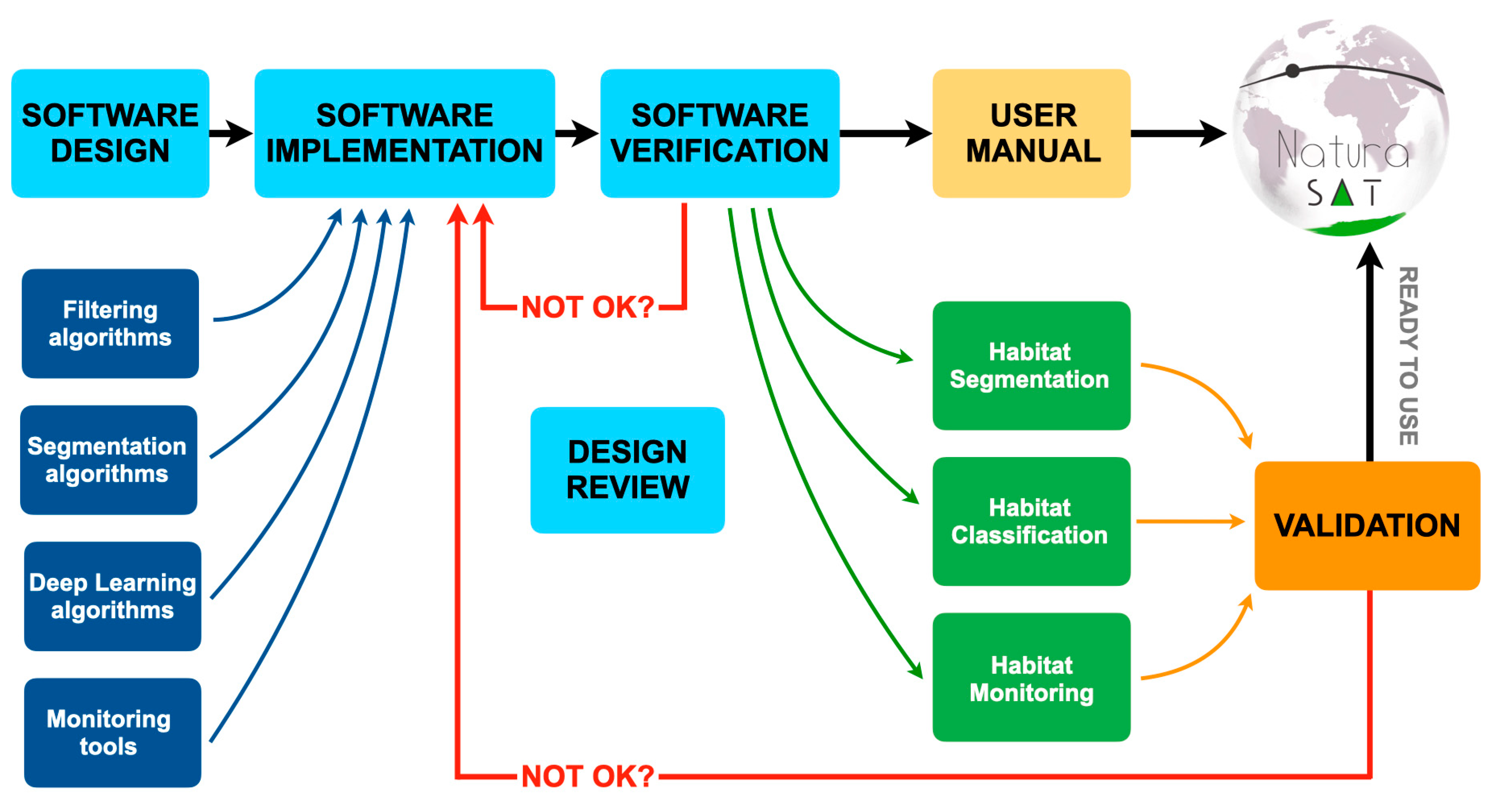
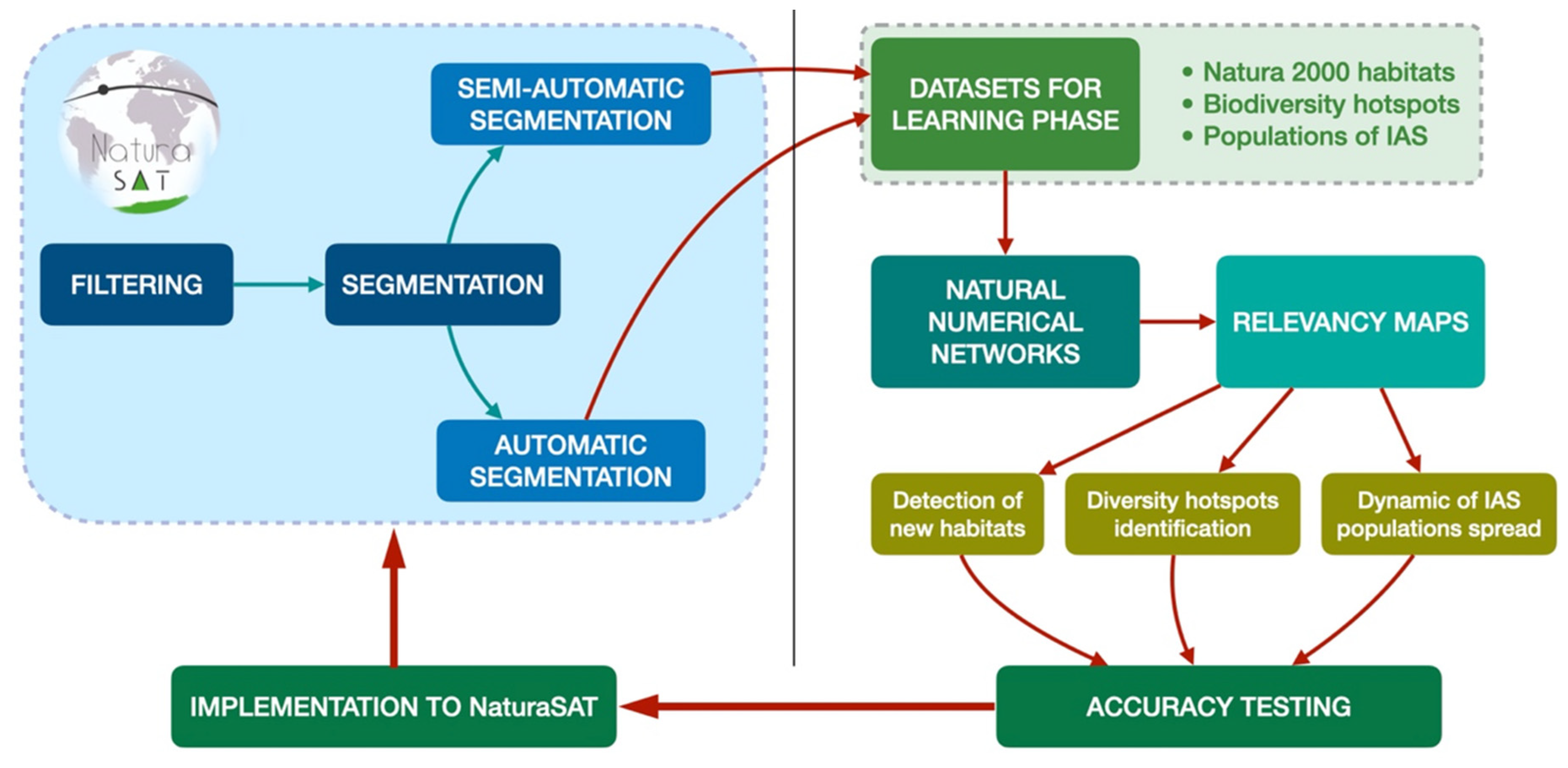
• Image filtering tool provides filtering methods based on linear, nonlinear and curvature based diffusion.
• The semi-automatic segmentation tool provides the semi-automatic segmentation of selected habitats in various types of images (satellite, airborne, UAV).
• Automatic segmentation tool provides automatic segmentation of selected habitats in various types of images (satellite, airborne, UAV).
• The monitoring tool provides methods for measuring habitat quality and habitat area.

Intensive cooperation between botany field scientists, mathematicians, and software developers has been ongoing during software development. The flowchart of development phases is illustrated in Figure 1. New methods for classification based on deep learning were developed and tested [18] and will be implemented into the software in the near future, as the “classification tool” that performs the classification of selected habitats and creates relevancy maps for chosen habitats. Together with the previously developed tools, we will also present and discuss the classification. In this section, we briefly introduce remotely sensed data sources used in the software (Section 2.1), implemented mathematical models (Section 2.2, Section 2.3 and Section 2.4), and the methodology of field data sampling and verification (Section 2.5). In the Results section, we describe verification accuracy and introduce some practical examples of software applications.

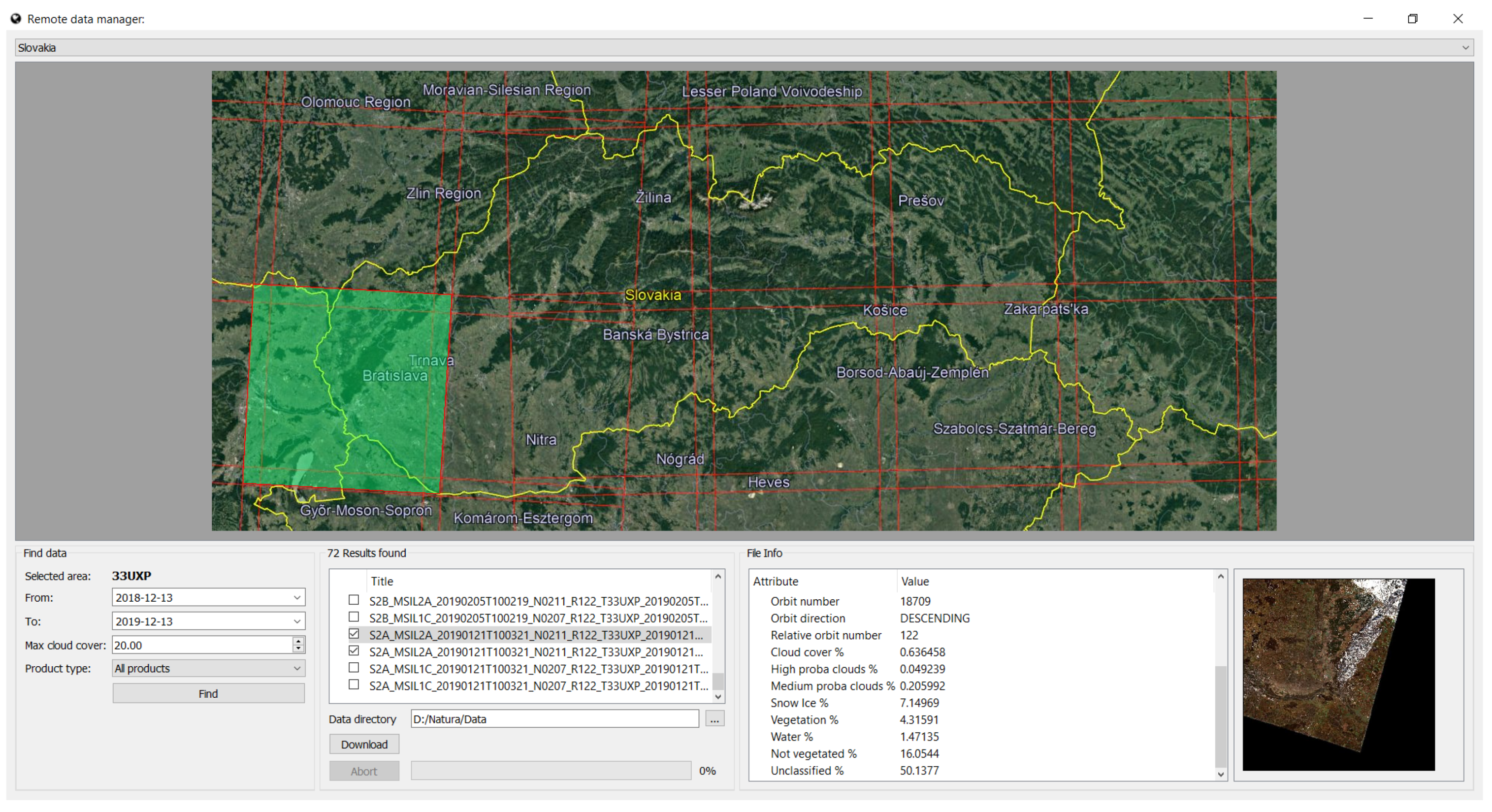
2.1. Remotely Sensed Data Used in the NaturaSat Software

The NaturaSat software works with multispectral data from the Sentinel-2 satellite, UAV, and airborne imagery and with every georeferenced picture format.

For the purpose of dynamic habitat monitoring, we implemented a functionality (remote download module) that allows a user to download Sentinel-2 data directly from our dedicated NaturaSat application. To access Sentinel-2 (both level-1C and level-2A/2Ap) data repositories, we use OpenSearch API on the Copernicus Open Access Hub.

The content of the request query link depends on user input in the user application interface. Since the NaturaSat project tasks are currently performed on data from the area of Slovakia, we divided this area according to the predefined Sentinel-2 tiling grid. The tiling grid contains approximately 56,500 tiles worldwide with defined code names, and 11 of them belong to the area of Slovakia (see Figure 2 top section). We use the code names for the identification of the user-selected area. Each tile represents an area of 100 × 100 km² in ortho-images in UTM/WGS84 projection.

A user can select one of the available tiles covering Slovakia and two dates defining a scope of data-sensing dates in the application interface. Since our segmentation algorithms are designed for optical data of sufficient quality, the user is able to select maximal cloud coverage (in %) and product type (all products, level-2A/2Ap or level-1C). After the user’s selection of all parameters, an API request is constructed. This request is sent to Copernicus Open Access Hub API, which returns the result as an XML file, including the list of nodes of every product stored in the data hub archive that fulfills the search query. An XML file is parsed, and results are shown to the user in the form of a list of product filenames. When one of the files is selected by the user, the extended information about the product is shown, e.g., percent coverage of clouds, snow, water, etc. The returned XML result file contains a preview image request url for every file. This url is used to show a quick preview of data to allow the user to see the quality of the image before downloading. The user can choose a destination directory to store the downloaded files. When the user clicks on the download button, all files with checked checkbox controls are downloaded to this directory. The remote download module (see Figure 2) works as a separate component of the NaturaSat application and does not block any other module during the download process. This allows the user to download multiple files while working with other application components. When the downloading process is finished, the user obtains information about the successful finalization of the process. Consequently, the user can load the downloaded data to the NaturaSat application for further processing.

2.2. Habitat Distribution

For assessing habitat distribution, two different approaches are commonly used—object-based and pixel-based approaches—and NaturaSat software supports both. The object-based approach is represented by segmentation methods where exact habitat boundaries are found semi-automatically by expert or automatically, starting from the georeferenced phytosociological relevé.

The main idea of our segmentation method is the usage of the suitable velocity vector field, utilizing smoothed image information, which drives the evolving curve automatically to the boundaries of segmented habitat. The vector field is constructed by using the pre-smoothed image intensity gradient as an edge indicator. Its magnitude is an input of the scalar edge detector function. Then the (negative) gradient of the edge detector function is projected to the curve normal, and the overall curve motion is regularized by using the local curvature of the evolving curve [19,20].

The NaturaSat software uses semi-automatic and automatic satellite image segmentation methods based on evolving planar curves [21,22]. Both methods represent efficient and robust segmentation tools when an “initial estimate” of the desired area is available. This is the case in Natura 2000 habitat segmentation, where the point-wise estimate of habitat occurrence is available in vegetation databases [23,24]. Thus, developed software tools allow focusing the Sentinel-2 image to the selected habitat occurrence data point, e.g., phytosociological relevé, or to the user-defined area, and then allow the user to perform semi-automatic or automatic segmentation by evolving the initial curve, either in the form of a straight line (semi-automatic segmentation) or in the form of a small circle (automatic segmentation).

The final mathematical model is given by the corresponding nonlinear intrinsic partial differential equation, which is discretized and solved numerically by the flowing finite volume method [25,26].

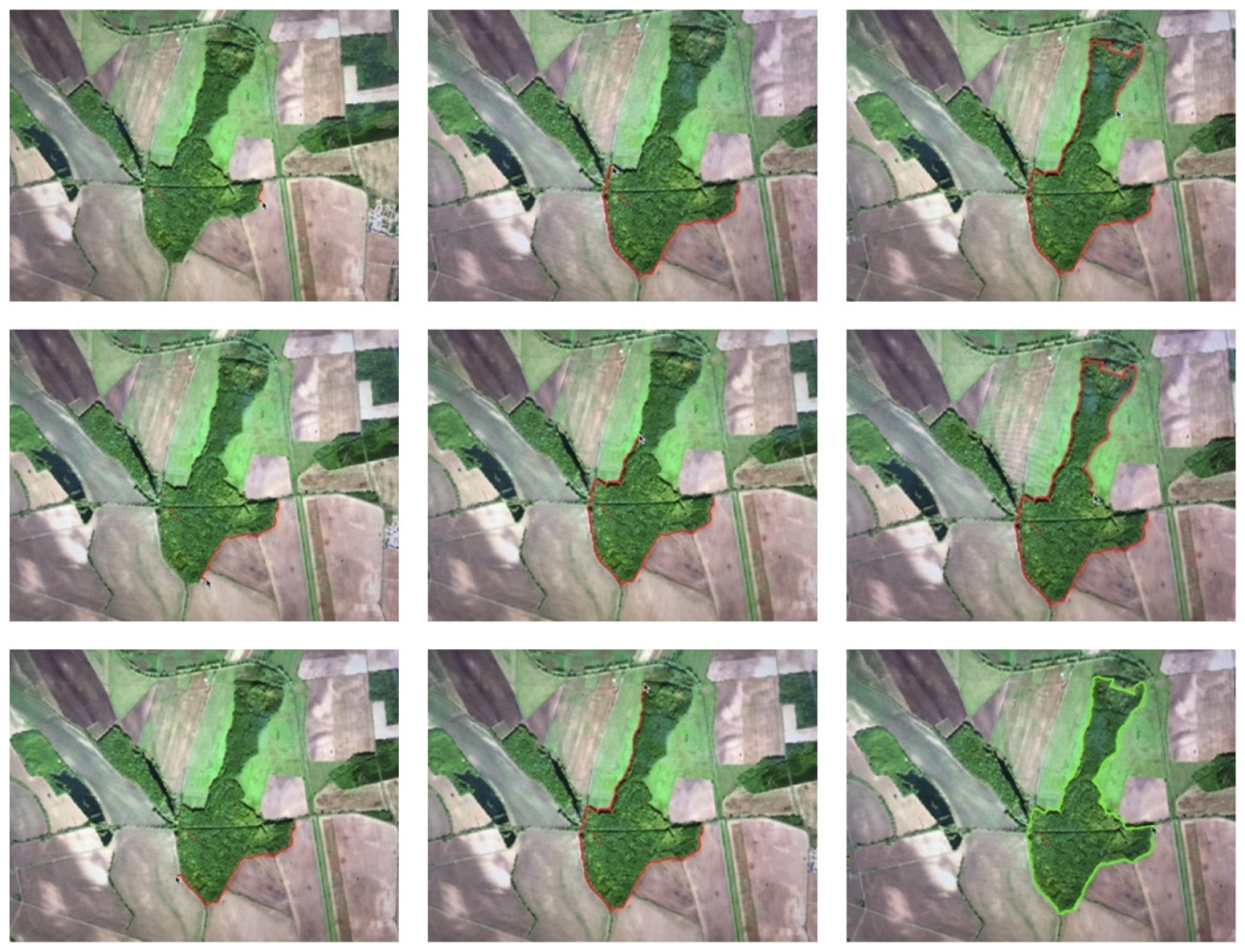
2.2.1. Semi-Automatic Segmentation

In the case of the semi-automatic segmentation, the user clicks the mouse at some correctly chosen point on the habitat boundary and drags the mouse along the expected habitat boundary—the algorithm always connects the first clicked point with the last mouse position, constructs the initial curve between them and in real-time adjusts this line to the habitat border by using the numerical scheme [21,27]. When the user is satisfied with the detected borderline, they click the mouse again, and that portion of segmentation is finished. Then the user can iterate this process to improve the boundary curve, as is illustrated in Figure 3 and Figure 4 and video in Supplementary Material Video S1.

2.2.2. Automatic Segmentation

This software tool is based on a mathematical model and its implementation of the time evolution of closed planar curves in the Lagrangian formulation. A detailed description of the mathematical model, numerical implementation, and numerical experiments showing the behavior of the developed method are presented by Mikula et al. [22]. The automatic segmentation could start from the user-defined initial curve (Figure 5, see also Supplementary Material Video S2) or from the phytosociological relevé representing the current habitat or plant community.

2.3. Habitat Classification and Relevancy Maps

The pixel-based approach is represented by relevancy maps based on a new deep learning method called natural numerical network (the method is presented in Mikula et al. [18]). The vector of computed values in all optical bands (mean, maximal, minimal, standard deviation) creates pixel characteristics that are used by the natural numerical network to classify the pixel within a habitat with certain relevancy (for details [18]). The method produces a so-called relevancy map in which the greyscale intensity of every pixel represents habitat occurrence relevancy. This approach allows habitats to be detected in degraded conditions (medium or low relevancy should show habitats with fewer diagnostic species). It is also sensitive to transitional habitat types that have high relevancy values for two different habitats. The case study presented here is based on training dataset containing 30 segmented areas of 91E0 habitat, 29 areas of 91F0, 32 areas of 91G0 and 34 areas of 9110 habitats. The Sentinel-2 data from 9 September 2018, covering Western Slovakia, were used for learning phase and computation of relevancy maps.

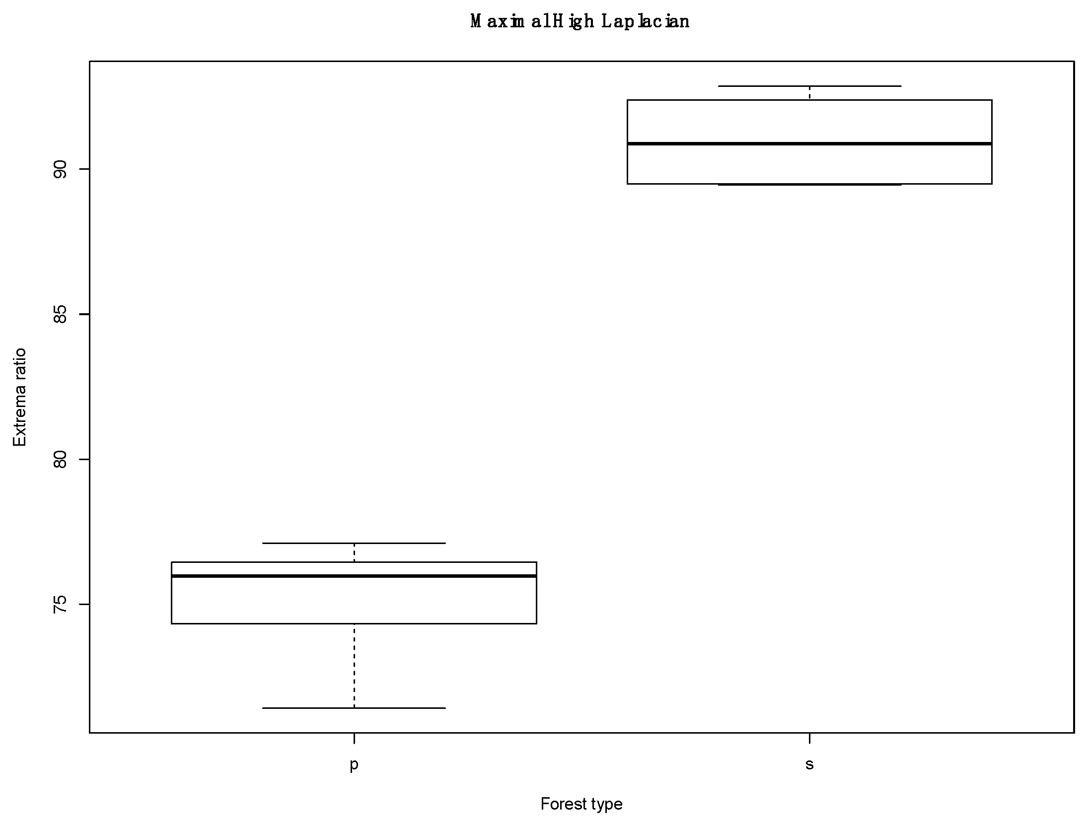
2.4. Distinguishing between Natural and Managed Habitats

In the case of forest habitats, there are some specific situations where the same tree species forms priority Natura 2000 habitats (e.g., Populus sp. in 91E0 habitat), but are also found as plantations. A new criterion, the relative high Laplacian (RHL), was developed and implemented into NaturaSat software to detect structural differences between such forests. Relative high Laplacian is given by the number of pixels where the Laplace operator, applied to image intensity, is high. In our case, we compute discrete Laplacian as the standard finite difference numerical approximation of the sum of second derivatives of image intensity values in the pixel.

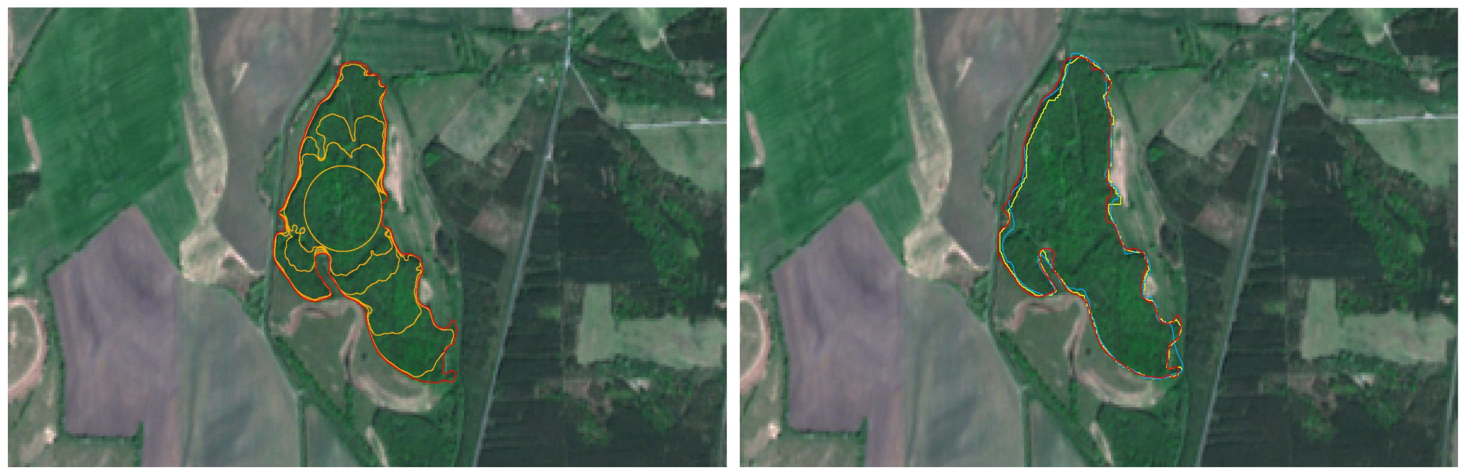
2.5. Testing and Validation of Image Segmentation

Two Natura 2000 habitats and plots (areas) suitable for testing and tuning parameters of semi-automatic and automatic segmentation algorithms were selected, as follows: “91F0 Riparian mixed forests of Quercus robur, Ulmus laevis, and Ulmus minor, Fraxinus angustifolia or Fraxinus excelsior along the great rivers” and “4070 * Bushes with Pinus mugo and Rhododendron hirsutum (Mugo-Rhododendretum hirsuti)” sampled in the field during vegetation seasons 2018–2019. Also, various Sentinel-2 optical band combinations at various dates were explored in order to find whether selected habitats are distinguishable in the Sentinel-2 optical data. The results of semi-automatic and automatic segmentations were compared visually and quantitatively with the GPS tracks obtained in the field.

For this quantitative comparison of two curves, we use the classical (maximal) Hausdorff distance and the so-called mean Hausdorff distance, which are general tools for computing the distance of curves, surfaces, and even more complicated geometrical continuous or discrete objects [21,22].

2.6. Habitat Monitoring

Our Natura 2000 habitat-monitoring approaches are based on semi-automatic and automatic segmentation algorithms used to monitor habitat quality and area evolution, respectively. The dynamic habitat quality monitoring used the Sentinel-2 image characteristics—values in all optical bands (mean, maximal, minimal, standard deviation) together with normalized difference vegetation index (NDVI) and RHL indexes.

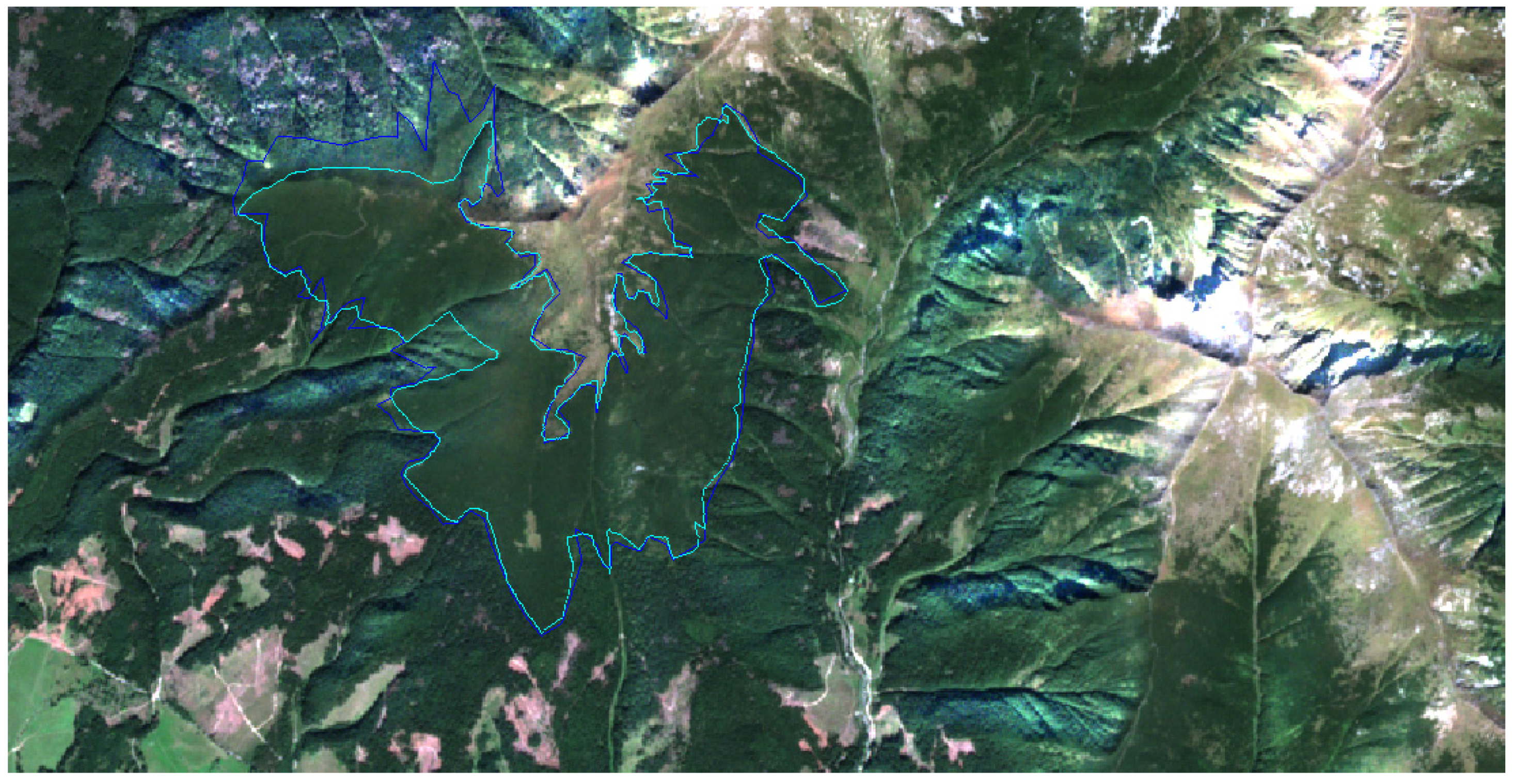
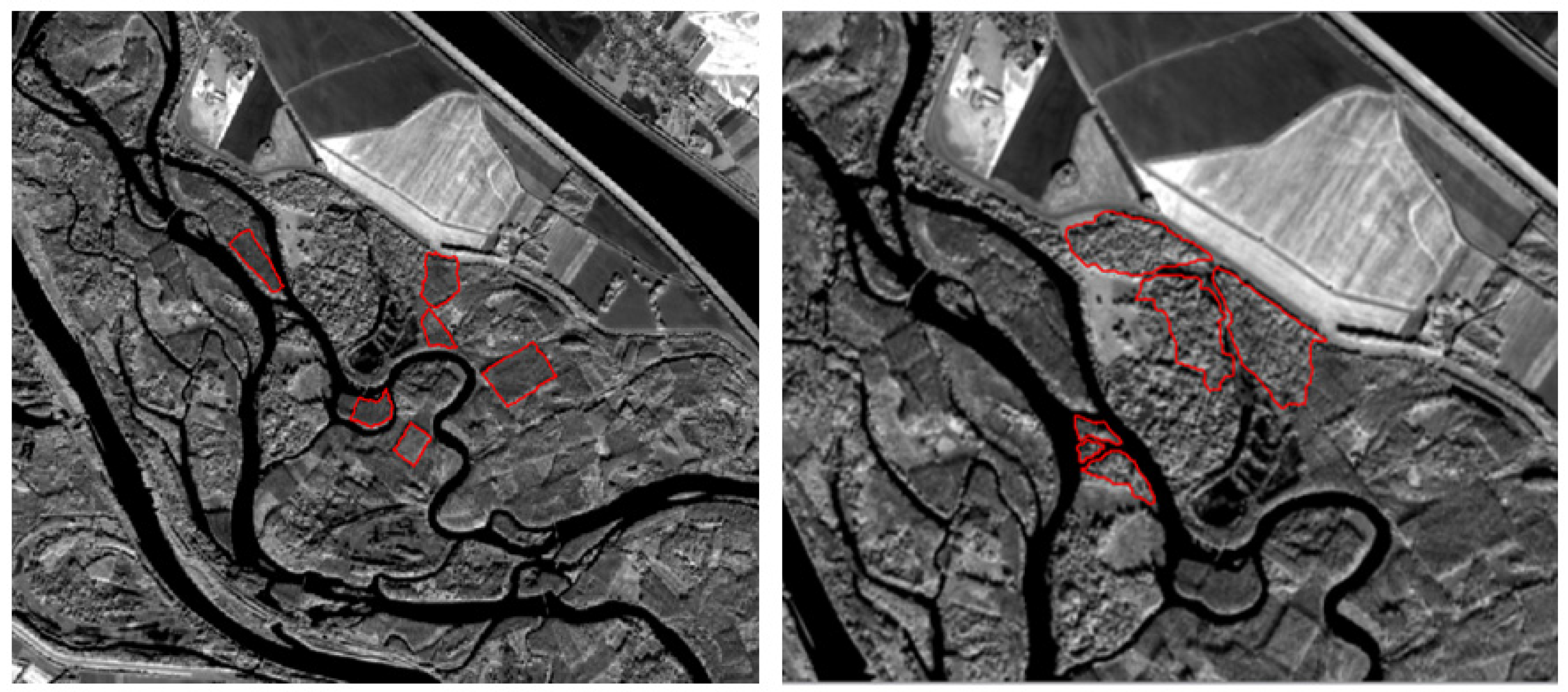
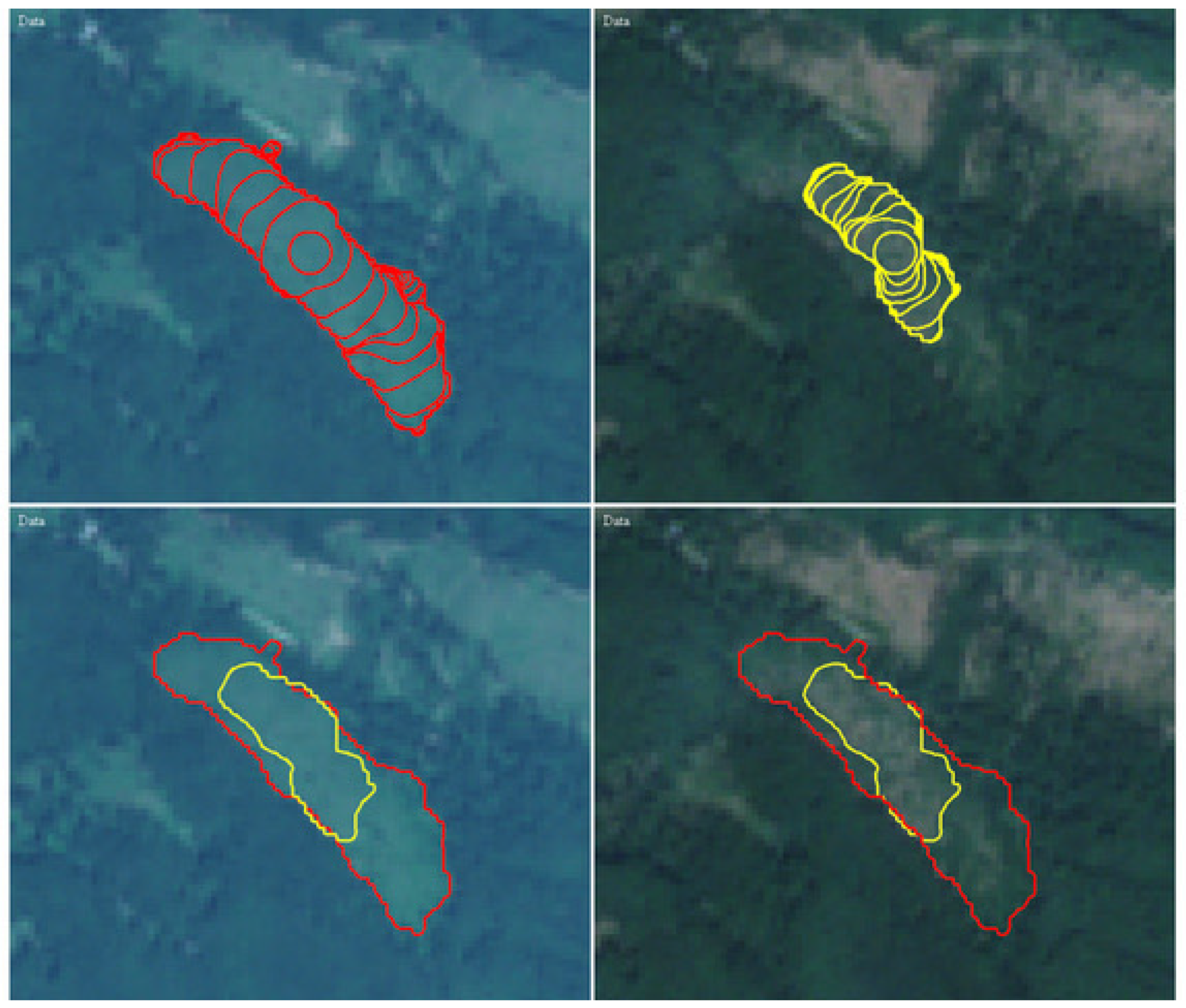
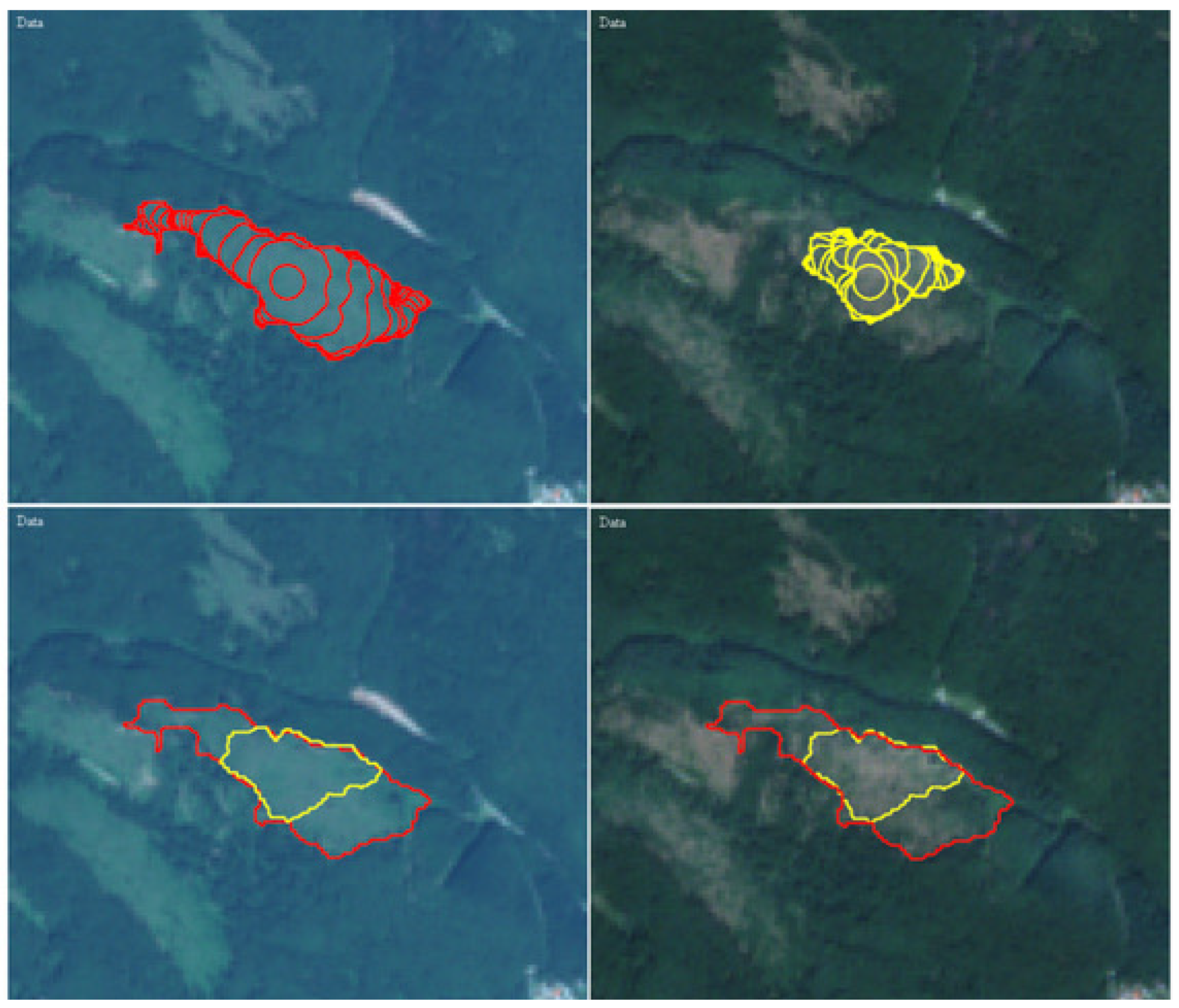
2.6.1. Spatio-Temporal Change Monitoring

The method developed for dynamic area change monitoring in Sentinel-2 dynamic data is based on the automatic segmentation method provided in different time periods. The segmentation model parameters were tuned to get the best possible area segmentation in the original data. Then we used the same model parameters for the segmentation in the updated data to get a segmentation of the area of the same habitat in the updated data. These two segmentations were quantitatively compared by means of Hausdorff distance, perimeter, area, and isoperimetric ratio (shape index) values.

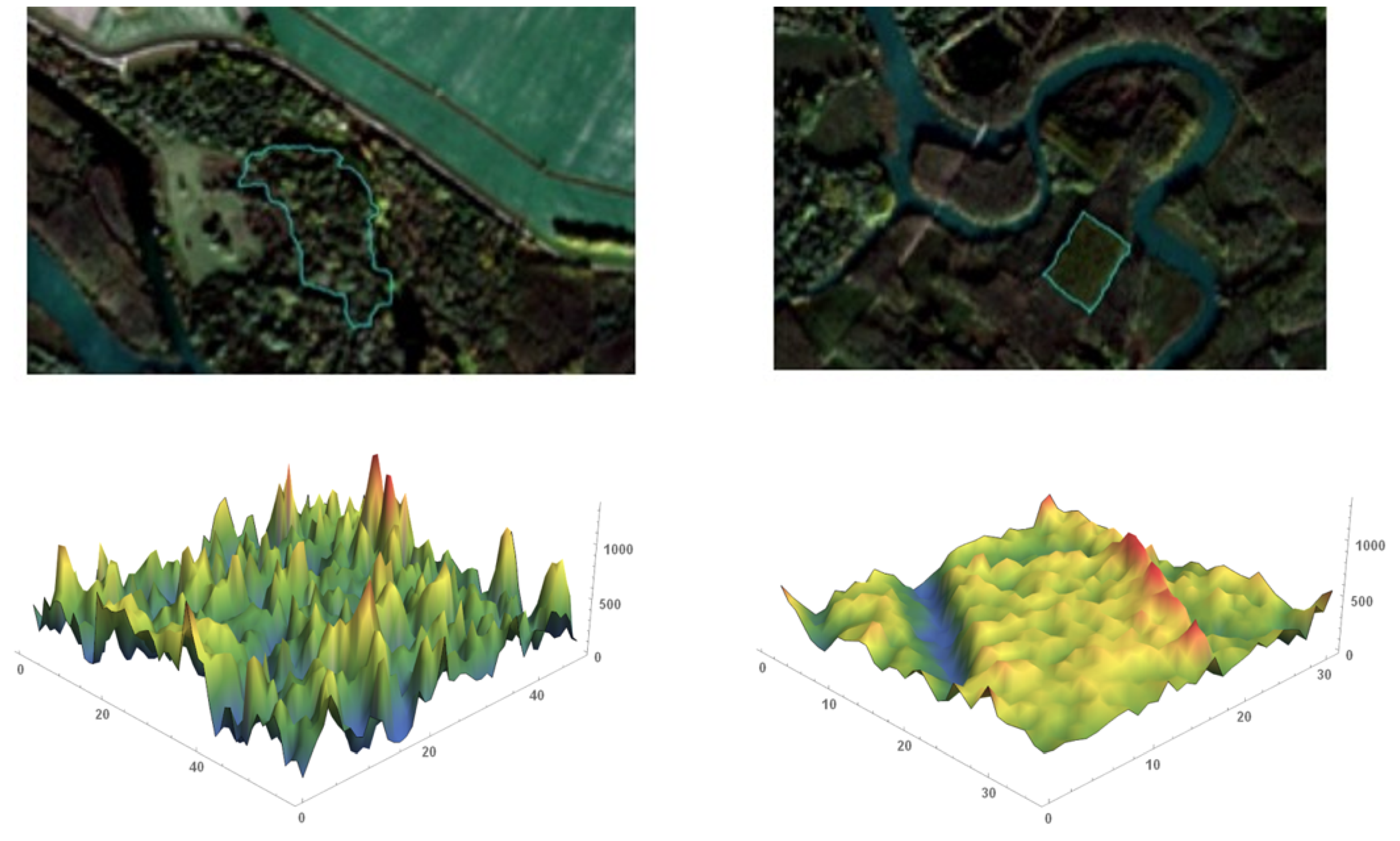
2.6.2. Habitat Quality Monitoring

The quality monitoring of habitats within NaturaSat software is based on comparing optical band values (mean, maximal, minimal, standard deviation, and NDVI) inside the same segmented area on different dates. During vegetation season 2019, localities with recent on-going changes were explored. Mountain spruce forests affected by bark beetle outbreak or clear-cuts were semi-automatically segmented. Grassland habitats affected by succession were segmented as well. The optical band characteristics were computed using NaturaSat software in the original data from 2016 and in the updated data from 2019. These two datasets were compared by paired t-tests (in R-software implementation, [28]) to verify the significance of observed changes.

3. Results

3.1. Habitat Distribution

The “91F0 Riparian mixed forests of Quercus robur, Ulmus laevis, and Ulmus minor, Fraxinus angustifolia or Fraxinus excelsior along the great rivers” habitat was selected due to its highest importance at both the Slovak and European level. It is a Natura 2000 priority habitat, and is endangered according to the red list of European habitats [29]. Despite this fact, riparian forests are often intensively managed by clear-cuts and replaced by monodominant stands of alien tree species (e.g., Canadian poplars). The riparian forests are among the most fragmented forest habitats in Slovakia, which were widespread in the alluvia of lowland rivers from the Neolithic era to the 12th century.

Forest areas with simple, as well as complicated, area shapes, with diverse borders, were chosen, which were thus suitable for testing the ability and performance of the developed segmentation methods. The forest fragments were surrounded by crop fields, meadows, river branches, roads, and different forest types. Some of the chosen riparian forests have a strict border, and some of them contain natural shrub edge (ecotone) zones. During the vegetation season 2018, twenty-four of the most important localities of riparian forests in Western Slovakia were visited by botanists, and their boundaries were tracked in the field with a GPS device. In the case of problems in the field, mainly due to flooded parts of forests where it was impossible to walk the entire border, some GPS tracks were corrected in the Google Earth Pro software. Afterwards, all these areas were semi-automatically or automatically segmented, and the mean and maximal Hausdorff distances of the GPS tracks and segmentations are given in

Table 1. The list of 91F0 riparian mixed forests localities with the mean and maximal Hausdorff distances of semi-automatically segmented and GPS-tracked boundaries.

Habitat	Locality Code	Mean Hausdorff Distance	Maximal Hausdorff Distance
91F0	bogdalickyvrch1	8.3785	25.1905
91F0	bogdalickyvrch2	7.5773	27.8022
91F0	bogdalickyvrch3	6.7352	35.5152
91F0	bogdalickyvrch4	7.1754	36.9335
91F0	brestovany1	8.8597	28.5780
91F0	brestovany2	14.2629	83.2185
91F0	brestovany3	7.7355	24.6512
91F0	brestovany4	8.9412	26.6053
91F0	dedovejamy1	9.9970	86.1185
91F0	dedovejamy2	11.7609	53.6198
91F0	dedovejamy3	14.0657	57.6020
91F0	dedovejamy4	10.5434	39.9949
91F0	feldskyles	11.3289	60.6908
91F0	feldskyles2	14.0136	44.1078
91F0	suchohrad	5.4751	18.2485
91F0	suchohradsever	6.3606	25.7611
91F0	suchohradTP	20.4569	172.1070
91F0	suchohradzahradzou	14.9159	40.0650
91F0	vysokaprimorave	14.6520	56.1716
91F0	vysokaprimorave2	19.5480	213.7380
91F0	vysokaprimorave3	19.7037	95.0065
91F0	vysokaprimorave4	11.9635	62.0790
91F0	zavod1	12.8527	37.4885
91F0	zavod2	8.3211	39.3252
91F0	Average	11.4844	57.9424

.

As we can observe from Table 1, the mean Hausdorff distance is, on average, 11.48 m, which is very close to the pixel resolution (10 m) of the Sentinel-2 data. This means that by using the developed semi-automatic segmentation method, we can detect 91F0 * habitat borders as accurately as the image resolution allows. The maximal Hausdorff distance is, on average, about 58 m, which represents 5–6 pixels. The highest differences are found in the areas with “ecotone zones”, where tree-dominated riparian forests are connected to surrounding meadows or fields by shrub-dominated zones. During the field GPS tracking, these zones were usually excluded from habitat areas, while, by segmentation, we included them due to a similarity in the forest and “ecotone zone” colors.

The automatic segmentation of selected localities of the 91F0 habitat was consequently compared with the semi-automatic segmentation and GPS tracks. The results are presented in Figure 5 and

Table 2. Examples of 91F0 habitat localities with the mean and maximal Hausdorff distances of automatically and semi-automatically segmented curves and automatically segmented curves and GPS-tracked boundaries.

		Automatic Versus Semi-Automatic		Automatic Versus GPS Track
Habitat	Locality Code	Mean Hausdorff Distance (m)	Max. Hausdorff Distance (m)	Mean Hausdorff Distance (m)	Max. Hausdorff Distance (m)
91F0	suchohradzahradzou	6.8	27.2	12.4	39.2
91F0	moravskyjan	10.7	63.9	10.8	50.4
91F0	vysokaprimorave4	8.5	51.9	11.7	49.9

. Two types of segmentation methods gave results with a mean Hausdorff distance less than the pixel resolution of the Sentinel-2 data, which means that automatic segmentation can effectively substitute semi-automatic segmentation, especially in areas that are densely covered by phytosociological relevés, which could serve as segmentation starting points.

The sites that are dominated by Pinus mugo represent habitats of European importance. Pinus mugo is generally considered to be a heliophilous pioneer species, but it is often found in extreme sites, to which it has been relegated by other competitors. This species creates a conspicuous krummholz zone, above the tree line, in the Central European mountains. In the past, it was affected by shepherds who eliminated the vegetation to expand pastures.

The boundaries of bushes with Pinus mugo were tracked in the field by the GPS device, during the vegetation season 2018, in various mountain ranges in Slovakia—Malá Fatra Mts, Západné Tatry Mts, Nízke Tatry Mts, Chočské vrchy Mts and Oravské Beskydy Mts. The habitat usually forms large areas with diversified shapes, discontinued by avalanche gullies, small mountain creeks, or glacially formed moraines. This fact implies that the field mapping of habitat borders in rugged high-altitude terrain is very complicated and time consuming. Using the satellite image segmentation methods is thus a very promising and efficient way of monitoring this habitat. Samples of localities in the Western Tatra mountain range, with borders given by the GPS tracking and segmentation, is shown in Figure 6. In

Table 3. The list of 4070 * bushes with Pinus mugo localities with the mean and maximal Hausdorff distances of semi-automatically segmented and GPS-tracked area boundaries.

Habitat	Locality Code	Mean Hausdorff Distance	Max. Hausdorff Distance
4070	choc20	19.1041	170.9960
4070	NT4	13.2219	83.2163
4070	NT5	14.3449	70.0201
4070	NT6	11.3362	51.2578
4070	NT8	14.7244	49.7035
4070	NT10	28.3386	336.1420
4070	orava13	10.6748	52.9471
4070	orava14	16.8741	116.0220
4070	ZT16	8.9677	86.7985
4070	ZT18	44.7946	413.2960
4070	MF1	3.6621	21.7807
4070	MF2	8.2804	88.0855
4070	MF3	11.3811	131.1500
4070	MF4	5.7333	20.6663
4070	MF5	15.3571	81.2460
4070	MF6	8.1688	59.4718
4070	MF7	6.7400	53.6128
4070	MF8	8.6118	79.3601
4070	Average	13.9064	109.2096

, we report the quantitative comparison of the GPS tracks and segmentation results.

As we can observe in Table 3, the average mean Hausdorff distance of the GPS tracked and semi-automatically segmented curves of bushes with Pinus mugo areas is 13.9 m, which is close to the Sentinel-2 optical data pixel resolution (10 m). The maximal Hausdorff distances are bigger than those observed for the riparian forests (see Table 1). Bushes with Pinus mugo grow in large areas, connected with the mountain spruce forests. Some extreme values of the maximal Hausdorff distance, for the localities ZT18 and NT10, are caused by the “ecotone zones”. The semi-automatic segmentation and GPS track curves of such localities are shown in Figure 6. The “ecotone zones” between the sites that are dominated by Pinus mugo and mountain spruce forests, often represent wide areas near the timberline that represent a transition in life form dominance, based on macro-climatic conditions. Timberline is a zone that is naturally very diverse, depending on the geological bedrock, relief type, exposition, wind conditions, and other factors reflecting all environmental conditions. Such transition zones are usually hard to classify, even subjectively by expert knowledge. Nevertheless, we see strong potential for the identification of the 4070 * habitat, by using the segmentation of the Sentinel-2 optical data. It allows a necessary simplification that helps determine the sharp edges in the images and avoid a subjective bias.

3.2. Distinguishing between Natural and Managed Habitats

For testing the possibility of distinguishing between 91E0 floodplain forests and poplar plantations, relative high Laplacian was calculated for six segmented polygons of 91E0 floodplain forests and six polygons of plantations (Figure 7). The values of the relative high Laplacian were compared (t-test, R-software) and visualized for model localities (Figure 8) and for the whole dataset, using a boxplot (Figure 9).

3.3. Habitat Classification and Relevancy Maps

For a demonstration of a relevancy map, the Sentinel-2 data for Western Slovakia, with the grid tile code 33UXP, and sampling date 10.9.2018, were selected. The relevancy map was computed for the 91F0 habitat, and compared with semi-automatic and automatic segmentation and the position of the phytosociological relevés representing this habitat. The relevancy maps from two different locations are depicted on the right side in Figure 10. White (bright) colors represent areas with a high relevancy of habitat classification and, on the contrary, the black (dark) color represent areas with low or zero relevancy. All the segmented habitat areas were identified by the relevancy map, as well as the locations of phytosociological relevés.

3.4. Habitat Monitoring

3.4.1. Dynamic Area Change Monitoring

For the testing and application of the dynamic monitoring method, grasslands (6510 habitat) in the Malé Karpaty-protected landscape area (PLA) from July 2015 (so-called original data) and August 2019 (called updated data), where significant changes occurred due to succession (Figure 11 and Figure 12), were chosen. We used automatic segmentation, as described in the Methods section. In

Table 4. Characteristics of the final segmentation curves from Figure 11 final segmented areas, showing their difference in area, perimeter, isoperimetric ratio and classical (HD) and mean (MHD) Hausdorff distances of two segmentation curves.

	2015	2019	Differences
Area [m2]	79,068.1	30,668.1	48,400.0
Perimeter [m]	1682.53	882.65	799.88
Isoperimetric ratio	0.350982	0.494664	0.143682
HD [m]			186.67
MHD [m]			61.61

and

Table 5. Characteristics of the final segmentation curves from Figure 12 final segmented areas showing their difference in area, perimeter, isoperimetric ratio and classical (HD) and mean (MHD) Hausdorff distances of two segmentation curves.

	2015	2019	Differences
Area [m2]	94,188.9	42,565.2	51,623.7
Perimeter [m]	1978.64	1021.37	957.27
Isoperimetric ratio	0.302327	0.512739	0.210412
HD [m]			230.83
MHD [m]			74.79

, we report the characteristics of the final segmentation curves in the original and updated data, showing their significant differences. We also report the Hausdorff distances of the final segmentation curves. We observe that the comparison of the final segmentation curves, from the original and updated data, enables us to indicate the abrupt changes in the habitat area and perimeter, and thus this can serve as a feasible monitoring tool for the habitat state change.

3.4.2. Habitat Quality Monitoring

Two sets of optical band characteristics, computed using the NaturaSat software (the first in the original data from 2016 and the second in the updated data from 2019), for segmented areas, were compared by paired t-tests (in R-software implementation). Significant changes were observed in the number of optical band characteristics. A list of the standard deviation values of image intensity, marking their significance in the case of a bark-beetle outbreak, clear-cut, and succession, is presented in

Table 6. A list of band characteristics used for the description of qualitative habitat changes. Characteristics that changed significantly between original and updated data are marked by an X mark.

Band Characteristic	Bark Beetle Outbreak	Clear-Cut	Succession
	Significance
B02-Blue_Std	X	.	.
B03-Green_Std	.	X	.
B04-Red_Std	.	.	.
B05-Vegetation classification_Std	.	.	.
B06-Vegetation classification_Std	X	X	.
B07-Vegetation classification_Std	.	.	.
B08-Near infrared_Std	X	.	X
B09-Water vapour_Std	.	.	X
B8A-Vegetation classification_Std	.	.	.

. The selected optical band characteristics reflect the significantly qualitative changes of habitats in the segmented regions. The simplest was the detection of clear-cuts, followed by the bark-beetle outbreaks.

4. Discussion

Our powerful unique software, NaturaSat, serves as the primary tool for implementing new approaches into habitat mapping and monitoring [21,22,27]. This tool integrates the knowledge of botany field scientists, mathematicians, and software developers, focusing on habitat use and nature conservancy, with the Natura 2000 network as one of the most important tools at the European level (habitats directive 92/43/EEC) [30,31]. Since direct human impact, together with climate warming, has profound consequences on biodiversity at local to global scales [32], there is an urgent need to identify and monitor spatio-temporal distribution, and the condition of habitats and important species populations, continuously. These challenges are reflected in many recent studies, from various habitats—peatlands [10,33]; wetlands [34]; hay meadows [35]. The Natura 2000 habitat [36,37,38,39] classifications, based on satellite data, were used mostly for large-scale vegetation mapping on the higher hierarchical level within individual habitat types. Habitats in the sense of Natura 2000 classification are complex vegetation units, consisting of different vegetation layers, and are defined by their species composition; thus, their correct recognition is challenging. The identification of some Natura 2000 habitats was possible when aerial photographs were used [39]. On the contrary, many remote sensing images (aerial or satellite) of the target vegetation types can have certain disadvantages, because of their potentially high cost, long cycles, and low resolution [12]. Therefore, proper resolution, at the highest possible level, is needed, depending on the intended goals.

Zlinszky et al. [39] tested airborne laser scanning as a source for mapping the conservation status of habitats and developing an automated method that calculates the Natura 2000 conservation status at a 0.5 m raster resolution. The surface texture (roughness), describing the vertical distribution of points within a neighborhood (related to vegetation canopy structure [34]), together with the digital terrain model, and its openness rasters [36], were calculated as a measure of the terrain texture, to enhance the linear features, sharpen the edges, and locate the minima and maxima in the terrain. Feilhauer et al. [37] found out that multispectral data may allow the combined mapping of discrete habitats and their local variability. These examples demonstrate the potential of remote sensing data in habitat exploration. Connecting these data to vegetation databases is a necessary subsequent step that was achieved by our approach.

The fact that updated satellite data are more accessible than aerial photos, and they are available for all parts of Europe and the world, makes our approach more applicable. However, using aerial photographs or UAV images is also possible within the NaturaSat software. Satellite images are sampled every five days, so there is a possibility to create a time series and monitor the habitats continuously.

Our aim was to create universal tools for such analyses, where various types of remote sensing data can be used, and a powerful deep learning method—natural numerical networks—can, after the learning phase, classify any target habitat, plant community, or phenomena, including invasive species spreading or biodiversity hotspots, and process the results as a relevancy map. The well-known metrics of species richness, diversity, and abundance are usually associated with habitat quality [40], and these are implemented in the NaturaSat software, together with the new RHL metric. By applying new methods of computation RHL within the images downloaded into the NaturaSat software, we can identify the potential conservation status of the target area.

The future dynamic development of the software will be based on the inclusion of new data for training datasets, verification in the field, and subsequent implementation of trained networks and segmentation databases into the software, as illustrated in Figure 13.

5. Conclusions

The NaturaSat software implements new powerful tools, such as the semi-automatic and automatic segmentation methods [21,22], and natural numerical networks. It is robust enough for vegetation scientists and nature conservationists to accurately extract target units’ borders, even at the habitat level. The automatic segmentation method involves minimal user intervention after parameter tuning, to achieve the desired accuracy. The Sentinel-2 optical bands’ resolution is suitable for exploring the forest and grassland habitats, with an accuracy close to the pixel resolution. Only the scarce small-scale habitats, with an area smaller than 100–200 square meters, cannot be detected; however, it is scale dependent, and thus, if there are UAV- or air-borne images used in the software, the limits are rapidly pushed. The semi-automatic segmentation can often be more accurate than GPS tracking by the fieldwork experts, since there is no influence of rugged relief and subjective bias on ecotone areas. The phenology affects and—at the same time—helps to distinguish between similar habitats (e.g., spring or autumnal aspect in the case of broadleaved forests). The deep learning algorithm that was developed for habitat classification within the NaturaSat software, can also be used in various botanical research tasks or in nature conservation practices, such as the identification of ecosystem services and conservation value [40]. The exact maps of the habitats obtained within the project can improve many further vegetation and landscape ecology studies. The NaturaSAT software is recently in the testing phase, and is available for academic users and nature conservationists worldwide, for non-commercial use only. For non-commercial software usage, do not hesitate to get in touch with the authors at [email protected] or [email protected].

References

1. Liu, P. A survey of remote-sensing big data. Front. Environ. Sci. 2015, 3, 45. [Google Scholar] [CrossRef] [Green Version]
2. Randin, C.F.; Ashcroft, M.B.; Bolliger, J.; Cavender-Bares, J.; Coops, N.C.; Dullinger, S.; Dirnböck, T.; Eckert, S.; Ellis, E.; Fernández, N.; et al. Monitoring biodiversity in the Anthropocene using remote sensing in species distribution models. Remote Sens. Environ. 2020, 239, 111626. [Google Scholar] [CrossRef]
3. Corbane, C.; Lang, S.; Pipkins, K.; Alleaume, S.; Deshayes, M.; García Millán, V.E.; Strasser, T.; Vanden Borre, J.; Toon, S.; Michael, F. Remote sensing for mapping natural habitats and their conservation status—New opportunities and challenges. Int. J. Appl. Earth Obs. Geoinf. 2015, 37, 7–16. [Google Scholar] [CrossRef]
4. Lausch, A.; Heurich, M.; Magdon, P.; Rocchini, D.; Schulz, K.; Bumberger, J.; King, D.J. A Range of Earth Observation Techniques for Assessing Plant Diversity. In Remote Sensing of Plant Biodiversity; Cavender-Bares, J., Gamon, J.A., Townsend, P.A., Eds.; Springer: Berlin/Heidelberg, Germany, 2020; Volume 13, pp. 309–348. [Google Scholar]
5. Ullerud, H.A.; Bryn, A.; Halvorsen, R.; Hemsing, L.Ø. Consistency in land-cover mapping: Influence of field workers, spatial scale and classification system. Appl. Veg. Sci. 2018, 21, 278–288. [Google Scholar] [CrossRef] [Green Version]
6. Chi, M.; Plaza, A.; Benediktsson, J.A.; Sun, Z.; Shen, J.; Zhu, Y. Big Data for Remote Sensing: Challenges and Opportunities. Proc. IEEE 2016, 104, 2207–2219. [Google Scholar] [CrossRef]
7. Rocchini, D.; Luque, S.; Pettorelli, N.; Bastin, L.; Doktor, D.; Faedi, N.; Feilhauer, H.; Féret, J.-B.; Foody, G.M.; Gavish, Y.; et al. Measuring β-diversity by remote sensing: A challenge for biodiversity monitoring. Methods Ecol. Evol. 2018, 9, 1787–1798. [Google Scholar] [CrossRef] [Green Version]
8. Pettorelli, N.; Bühne, H.S.T.; Tulloch, A.; Dubois, G.; Macinnis-Ng, C.; Queirós, A.M.; Keith, D.A.; Wegmann, M.; Schrodt, F.; Stellmes, M.; et al. Satellite remote sensing of ecosystem functions: Opportunities, challenges and way forward. Remote Sens. Ecol. Conserv. 2018, 2, 2056–3485. [Google Scholar] [CrossRef]
9. De Klerk, H.M.; Burgess, N.D.; Visser, V. Probabilistic description of vegetation ecotones using remote sensing. Ecol. Inform. 2018, 46, 125–132. [Google Scholar] [CrossRef]
10. Minasny, B.; Berglund, Ö.; Connolly, J.; Hedley, C.; De Vries, F.; Gimona, A.; Kempen, B.; Kidd, D.; Lilja, H.; Malone, B.; et al. Digital mapping of peatlands—A critical review. Earth-Sci. Rev. 2019, 196, 102870. [Google Scholar] [CrossRef]
11. Zellweger, F.; De Frenne, P.; Lenoir, J.; Rocchini, D.; Coomes, D. Advances in Microclimate Ecology Arising from Remote Sensing. Trends Ecol. Evol. 2019, 34, 327–341. [Google Scholar] [CrossRef] [Green Version]
12. Zhang, X.; Zhang, F.; Qi, Y.; Deng, L.; Wang, X.; Yang, S. New research methods for vegetation information extraction based on visible light remote sensing images from an unmanned aerial vehicle (UAV). Int. J. Appl. Earth Obs. Geoinf. 2019, 78, 215–226. [Google Scholar] [CrossRef]
13. Braun-Blanquet, J. Pflanzensoziologie: Grundzüge der Vegetationskunde, 3rd ed.; Springer: Wien, Austria, 1964; p. 865. [Google Scholar]
14. Chytrý, M.; Tichý, L.; Hennekens, S.M.; Knollová, I.; Janssen, J.A.M.; Rodwell, J.S.; Peterka, T.; Marcenò, C.; Landucci, F.; Danihelka, J.; et al. EUNIS Habitat Classification: Expert system, characteristic species combinations and distribution maps of European habitats. Appl. Veg. Sci. 2020, 23, 648–675. [Google Scholar] [CrossRef]
15. Landucci, F.; Tichý, L.; Šumberová, K.; Chytrý, M. Formalized classification of species-poor vegetation: A proposal of a consistent protocol for aquatic vegetation. J. Veg. Sci. 2015, 26, 791–803. [Google Scholar] [CrossRef]
16. Zhu, Y.; Zhang, Y.; Zu, J.; Wang, Z.; Huang, K.; Cong, N.; Tang, Z. Effects of data temporal resolution on phenology extractions from the alpine grasslands of the Tibetan Plateau. Ecol. Indic. 2019, 104, 365–377. [Google Scholar] [CrossRef]
17. Vanden Borre, J.; Paelinckx, D.; Mücher, C.A.; Kooistra, L.; Haest, B.; De Blust, G.; Schmidt, A.M. Integrating remote sensing in Natura 2000 habitat monitoring: Prospects on the way forward. J. Nat. Conserv. 2011, 19, 116–125. [Google Scholar] [CrossRef]
18. Mikula, K.; Kollár, M.; Ožvat, A.A.; Ambroz, M.; Čahojová, L.; Jarolímek, I.; Šibík, J.; Šibíková, M. Natural Numerical Networks for Natura 2000 habitats exploration by satellite data. Appl. Math. Model. 2021. submitted. Available online: https://arxiv.org/abs/2108.04327 (accessed on 19 August 2021).
19. Caselles, V.; Kimmel, R.; Sapiro, G. Geodesic active contours. Int. J. Comput. Vis. 1997, 22, 61–79. [Google Scholar] [CrossRef]
20. Kichenassamy, S.; Kumar, A.; Olver, P.; Tannenbaum, A.; Yezzi, A. Conformal curvature flows: From phase transition to active vision. Arch. Ration. Mech. Anal. 1996, 134, 275–301. [Google Scholar] [CrossRef] [Green Version]
21. Mikula, K.; Urbán, J.; Kollár, M.; Ambroz, M.; Jarolímek, I.; Šibík, J.; Šibíková, M. Semi-automatic segmentation of natura 2000 habitats in sentinel-2 satellite images by evolving open curves. Discret. Contin. Dyn. Syst. Ser. S 2021, 14, 1033–1046. [Google Scholar] [CrossRef] [Green Version]
22. Mikula, K.; Urbán, J.; Kollár, M.; Ambroz, M.; Jarolímek, I.; Šibík, J.; Šibíková, M. An automated segmentation of NATURA 2000 habitats from Sentinel-2 optical data. Discret. Contin. Dyn. Syst. Ser. S 2021, 14, 1017–1032. [Google Scholar] [CrossRef]
23. Šibík, J. Slovak Vegetation Database. In Vegetation Databases for the 21st Century; Dengler, J., Oldeland, J., Jansen, F., Chytrý, M., Ewald, J., Finckh, M., Glöckler, F., Lopez-Gonzalez, G., Peet, R.K., Schaminée, J.H.J., Eds.; Biodiversity & Ecology: Hamburg, Germany, 2012; Volume 4, p. 429. [Google Scholar]
24. Chytrý, M.; Hennekens, S.M.; Jiménez-Alfaro, B.; Knollová, I.; Dengler, J.; Jansen, F.; Landucci, F.; Schaminée, J.H.J.; Aćić, S.; Agrillo, E.; et al. European Vegetation Archive (EVA): An integrated database of European vegetation plots. Appl. Veg. Sci. 2016, 19, 173–180. [Google Scholar] [CrossRef] [Green Version]
25. Mikula, K.; Ševčovič, D. Evolution of plane curves driven by a nonlinear function of curvature and anisotropy. SIAM J. Appl. Math. 2001, 61, 1473–1501. [Google Scholar]
26. Mikula, K.; Ševčovič, D.; Balažovjech, M. A simple, fast and stabilized flowing finite volume method for solving general curve evolution equations. Commun. Comput. Phys. 2010, 7, 195–211. [Google Scholar] [CrossRef]
27. Ambroz, M.; Kollár, M.; Mikula, K. Semi-implicit scheme for semi-automatic segmentation in Naturasat software. In Proceedings of the 21th Conference on Scientific Computing, Vysoké Tatry-Podbanské, Slovakia, 10–15 September 2020; pp. 171–180. [Google Scholar]
28. R Core Team. R: A Language and Environment for Statistical Computing; R Foundation for Statistical Computing: Vienna, Austria, 2013. [Google Scholar]
29. Janssen, J.A.M.; Rodwell, J.S.; Criado, M.G.; Gubbay, S.; Haynes, T.; Nieto, A.; Sanders, N.; Landucci, F.; Loidi, J.; Ssymank, A.; et al. European Red List of Habitats, Part 2, Terrestrial and Freshwater Habitats; European Union: Luxembourg, 2016; p. 44. [Google Scholar]
30. Margules, C.R.; Pressey, R.L. Systematic conservation planning. Nature 2000, 405, 243–253. [Google Scholar] [CrossRef] [PubMed]
31. Weber, N.; Christophersen, T. The influence of non-governmental organisations on the creation of Natura 2000 during the European Policy process. For. Policy Econ. 2002, 4, 1–12. [Google Scholar] [CrossRef]
32. Pereira, H.M.; Leadley, P.W.; Proença, V.; Alkemade, R.; Scharlemann, J.P.W.; Fernandez-Manjarrés, J.F.; Araújo, M.B.; Balvanera, P.; Biggs, R.; Cheung, W.W.L.; et al. Scenarios for Global Biodiversity in the 21st Century. Science 2010, 330, 1496–1501. [Google Scholar] [CrossRef] [PubMed] [Green Version]
33. Rudiyanto; Minasny, B.; Setiawan, B.I.; Saptomo, S.K.; McBratney, A.B. Open digital mapping as a cost-effective method for mapping peat thickness and assessing the carbon stock of tropical peatlands. Geoderma 2018, 313, 25–40. [Google Scholar] [CrossRef]
34. Zlinszky, A.; Mücke, W.; Lehner, H.; Briese, C.; Pfeifer, N. Categorizing Wetland Vegetation by Airborne Laser Scanning on Lake Balaton and Kis-Balaton, Hungary. Remote Sens. 2012, 4, 1617–1650. [Google Scholar] [CrossRef] [Green Version]
35. Besnard, A.G.; Davranche, A.; Maugenest, S.; Bouzillé, J.B.; Vian, A.; Secondi, J. Vegetation maps based on remote sensing are informative predictors of habitat selection of grassland birds across a wetness gradient. Ecol. Indic. 2015, 58, 47–54. [Google Scholar] [CrossRef] [Green Version]
36. Doneus, M. Openness as Visualization Technique for Interpretative Mapping of Airborne Lidar Derived Digital Terrain Models. Remote Sens. 2013, 5, 6427–6442. [Google Scholar] [CrossRef] [Green Version]
37. Feilhauer, H.; Dahlke, C.; Doktor, D.; Lausch, A.; Schmidtlein, S.; Schulz, G.; Stenzel, S. Mapping the local variability of Natura 2000 habitats with remote sensing. Appl. Veg. Sci. 2014, 17, 765–779. [Google Scholar] [CrossRef]
38. Zlinszky, A.; Deák, B.; Kania, A.; Schroiff, A.; Pfeifer, N. Natura 2000 Habitat Quality mapping in a Pannonic salt steppe from full-waveform Airborne Laser Scanning. In Proceedings of the International Workshop on Remote Sensing and GIS for Monitoring of Habitat Quality, Vienna, Austria, 24–25 September 2014; pp. 130–134. [Google Scholar]
39. Zlinszky, A.; Deák, B.; Kania, A.; Schroiff, A.; Pfeifer, N. Mapping Natura 2000 Habitat Conservation Status in a Pannonic Salt Steppe with Airborne Laser Scanning. Remote Sens. 2015, 7, 2991–3019. [Google Scholar] [CrossRef] [Green Version]
40. Capmourteres, V.; Anand, M. “Conservation value”: A review of the concept and its quantification. Ecosphere 2016, 7, e01476. [Google Scholar] [CrossRef]
Figure 1. The diagram of development and functionalities of the NaturaSat software.
Remotesensing 13 03381 g001
Figure 2. User interface of the remote download module containing requested files with detailed information and preview image.
Remotesensing 13 03381 g002
Figure 3. An example of the semi-automatic segmentation showing consecutive building of the segmentation curve, the intermediate steps (from top left down to the bottom right) are in red, the final result is in green on bottom right.
Remotesensing 13 03381 g003
Figure 4. Semi-automatic segmentation of a part of the halophytic vegetation area on UAV data.
Remotesensing 13 03381 g004
Figure 5. Example of the automatic segmentation applied to the riparian forest Natura 2000 habitat in Záhorie PLA. Left: the evolution of the segmentation curve from the initial circle (around phytosociological relevé) to the final state. Right: the final automatic segmentation (red) together with the result of the semi-automatic segmentation (yellow) and the GPS track (light-blue).
Remotesensing 13 03381 g005
Figure 6. The locality with the highest maximal Hausdorff distance between semi-automatically segmented and GPS-tracked curves among sites with Pinus mugo (ZT 18). On the north-west habitat border, we can observe the “ecotone zone” that was included during field tracking (blue) and excluded by using of the semi-automatic segmentation (light-blue).
Remotesensing 13 03381 g006
Figure 7. Segments of poplar plantations (left) and Natura 2000 habitat 91E0 floodplain forests (right) in the area of Danube inland delta.
Remotesensing 13 03381 g007
Figure 8. Variability of the image intensity values inside natural forest area is high (left), which is expressed in high values of RHL, while in the plantation, (right) the image intensity is smoother, which is expressed in low values of RHL.
Remotesensing 13 03381 g008
Figure 9. Comparison of relative high Laplacian value for plantations (p) and 91E0 habitats (s). Boxplot graph represents median value (black line), first and third quartile (box), maximum and minimum (whiskers).
Remotesensing 13 03381 g009
Figure 10. Relevancy maps for the 91F0 habitat compared with segmentation curves (yellow), and phytosociological relevés location (red points). The values 0–1 represent a measure of relevancy of habitat occurrence from the highest (1) to lowest (0) probability. All pictures are standardly north oriented on upper side of the figure. The Sentinel-2 data from 9 September 2018, covering Western Slovakia, were used for learning phase and computation of relevancy maps.
Remotesensing 13 03381 g010
Figure 11. The example of grassland habitat segmentation. The top left image shows segmentation (red) in the original data from 2015. The top right image shows segmentation (yellow) in the updated data from 2019, where succession is visible. The bottom row compares visually the final segmented areas illustrated on both original and updated data.
Remotesensing 13 03381 g011
Figure 12. The second example of the grassland habitat segmentation. The top left image shows segmentation (red) in the original data from 2015. The top right image shows segmentation (yellow) in the updated data from 2019. The bottom row compares the final segmented areas before and after successional changes.
Remotesensing 13 03381 g012
Figure 13. A scheme showing workflow of dynamic development and using of NaturaSat software.
Remotesensing 13 03381 g013