Article

Remote Sensing of Pasture Degradation in the Highlands of the Kyrgyz Republic: Finer-Scale Analysis Reveals Complicating Factors

by
Monika A. Tomaszewska
1 and
Geoffrey M. Henebry
1,2,*
1
Center for Global Change and Earth Observations, Michigan State University, East Lansing, MI 48823, USA
2
Department of Geography, Environment, and Spatial Sciences, Michigan State University, East Lansing, MI 48824, USA
*
Author to whom correspondence should be addressed.
Remote Sens. 2021, 13(17), 3449; https://0-doi-org.brum.beds.ac.uk/10.3390/rs13173449
Submission received: 1 July 2021 / Revised: 24 August 2021 / Accepted: 26 August 2021 / Published: 31 August 2021
(This article belongs to the Special Issue Land Degradation Assessment with Earth Observation)

Abstract

:
Degradation in the highland pastures of the Kyrgyz Republic, a small country in Central Asia, has been reported in several studies relying on coarse spatial resolution imagery, primarily MODIS. We used the results of land surface phenology modeling at higher spatial resolution to characterize spatial and temporal patterns of phenometrics indicative of the seasonal peak in herbaceous vegetation. In particular, we explored whether proximity to villages was associated with substantial decreases in the seasonal peak values. We found that terrain features—elevation and aspect—modulated the strength of the influence of village proximity on the phenometrics. Moreover, using contrasting hotter/drier and cooler/wetter years, we discovered that the growing season weather can interact with aspect to attenuate the negative influences of dry conditions on seasonal peak values. As these multiple contingent and interactive factors that shape the land surface phenology of the highland pastures may be blurred and obscured in coarser spatial resolution imagery, we discuss some limitations with prior and recent studies of pasture degradation.

1. Introduction

The Kyrgyz Republic (Kyrgyzstan) is a small, highly mountainous nation of ~6.5 million in 2019, where more than 60% live in rural areas and where agropastoralism is the predominant land use [1]. Degradation of pasture resources in highly mountainous Kyrgyz Republic has been both widely reported [2,3,4,5,6,7,8] and disputed [9,10]. Many studies have attempted to detect land degradation in Central Asia by using remote sensing products based on finer temporal but coarser spatial resolution imagery [4,7,8,11,12,13,14,15,16]. While the finer temporal resolution products are better able to obtain clear views of the land surface, coarser spatial resolution products blend together heterogeneous surfaces. This blending or mixing is of particular concern in mountainous terrain, where differential insolation regimes arising from the interaction of aspect and slope generates microclimates that can accommodate distinct vegetation communities exhibiting different phenologies [3,17,18,19].
Untangling the differential influences of climate and human activity is complicated by coarser spatial resolution [7,14,20]. Pastoralism in Kyrgyzstan is characterized by transhumance, the seasonal movement of livestock to fresh pastures, and vertical transhumance in particular, where the herds are moved from low-elevation winter pastures near villages through transitional pastures in spring (and again in fall) to higher elevation summer pastures distant from settlements. This combination of spatial heterogeneity, terrain effects, and seasonality of pasture use presents challenges for detecting pasture degradation from coarser resolution remote sensing imagery. A further complication is presented by the high interannual variation in weather arising from the land-locked location of the country, its relatively high elevation, and regional climate change [12,21,22,23,24].
Here, we explore the pasture degradation question across rural Kyrgyz Republic using phenological metrics (phenometrics) derived from finer spatial resolution, but less frequent imagery (Landsat 30 m) linked to more frequent, but coarser spatial resolution products (MODIS 1 km) across 17 years (2001–2017). The phenometrics that we use here indicate the first seasonal peak in NDVI and the amount of thermal time (measured as accumulated growing degree-days calculated from land surface temperature time series) required to reach that peak NDVI. These phenometrics can be calculated for each pixel in each year for which there are sufficient, high-quality data and for which the joint time series exhibit sufficient seasonality to enable the modeling of the land surface phenology (LSP). Pasture degradation can be evaluated with phenometrics in a variety of ways, including trends, variation, extremes, and abrupt spatial and/or temporal shifts [12,20,25,26]. However, we are interested here in three questions about patterns that can complicate interpretation of patterns and trends: (1) What are the spatial patterns of the phenometrics as a function of distance from village center? (2) How do these patterns change as a function of elevation? and (3) How do these patterns change as a function of aspect?
Although we focus on the patterns of the temporal mean phenometrics during the study period, we also examine the patterns during two years with contrasting weather: hotter, drier 2007 versus cooler, wetter 2009. This study leverages the findings from prior studies [25,26] using the same approach to modeling land surface phenology and advances our understanding of the spatio-temporal dynamics of vegetation in the socio-ecological landscapes of montane Central Asia, specifically in the Kyrgyz Republic.

2. Materials and Methods
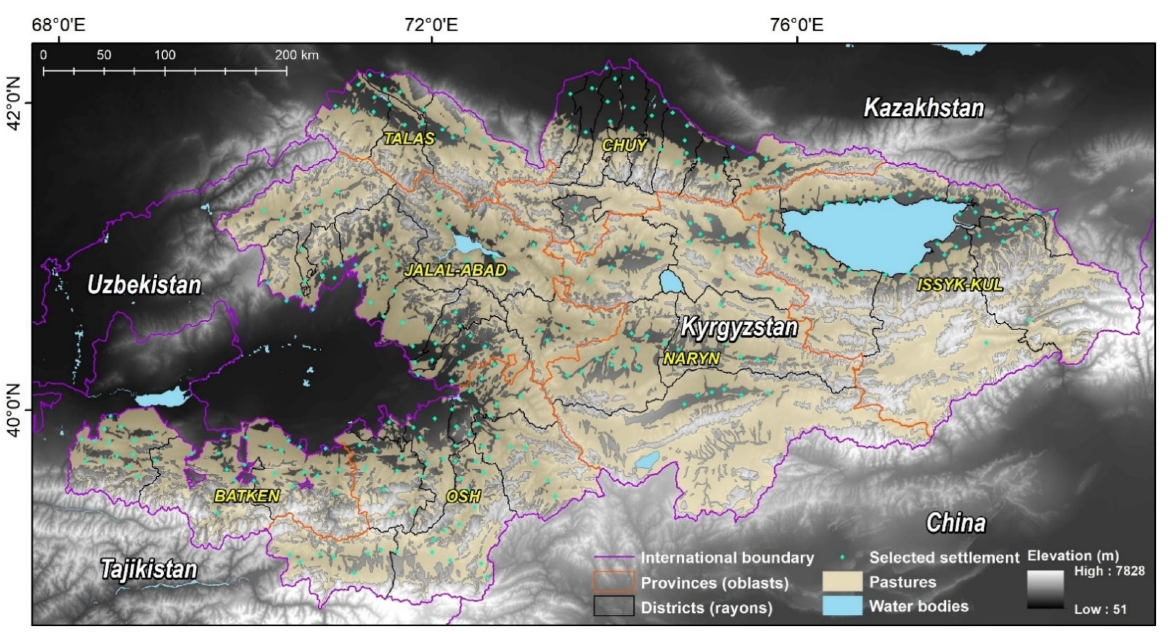
2.1. Study Area

The study area focuses on pasture lands within the territory of the Kyrgyz Republic that neighbors Uzbekistan (west), Kazakhstan (north), China (east and southeast), and Tajikistan (southwest) (Figure 1). The total area of the country is shy of 200,000 km2 (96% in land), and the 2019 population was about 6.5 million, according to the World Bank (https://data.worldbank.org/country/kyrgyz-republic; accessed on 20 June 2021). It is a highly mountainous country, where more than 56% of the territory lies above 2500 m and where the mountain ranges of the Tien Shan, Pamir, and Alatau cover more than 90% of the total land area [27]. Pastoral rangelands constitute 87% [1] of the agricultural lands in the Kyrgyz Republic. Less than 10% of the land is used for crops, while forests cover only about 5%. Our study period extends from 2001 through 2017. The Kyrgyz Republic is divided into seven provinces (oblasts)—Talas, Chuy (including the capital city, Bishkek), and Issyk-Kul in the northern part as well as Jalal-Abad, Naryn, Osh, and Batken in the southern part—and 40 districts (rayons).

2.2. Geospatial Data

The land surface phenology metrics (or phenometrics) and terrain information used for this study were supplied from our previous work [25], where a detailed description of data, its processing, and phenometrics calculation methodology can be found. We provide an overview here.
To calculate LSP metrics, we used two products: MODIS land surface temperature (LST) and Landsat surface reflectance NDVI.
We downloaded two tiles (h23v04 and h23v05) of 8-day MODIS Terra and MODIS Aqua Land Surface Temperature (MOD11A2/MYD11A2 V006) products at 1 km spatial resolution [31] from 2001 (MODIS/Terra) and from 2002 (MODIS/Aqua) up to the end of 2017. We merged tiles, removed poor quality pixels, converted units from Kelvin to °C, and reprojected data to Albers Conic Equal Area at 30 m spatial resolution using bilinear resampling.
The surface reflectance NDVI dataset from Landsat Collection 1 Tier 1 Level-1 Precision and Terrain (L1TP) of Landsat 5 Thematic Mapper (TM), Landsat 7 Enhanced Thematic Mapper Plus (ETM+), and Landsat 8 Operational Land Imager (OLI) was acquired for years 2001 to the end of 2017 from the USGS Earth Resources Observation and Science (EROS) Center Science Processing Architecture (ESPA) On-Demand Interface (https://espa.cr.usgs.gov/). We downloaded 13,285 images across 33 unique tiles (WRS-2 Paths 147–155 and Rows 30–33) which were already projected into Albers Conic Equal Area. We masked poor-quality pixels and applied an inter-calibration equation to adjust Landsat 5 TM surface NDVI and Landsat 7 ETM+ surface NDVI to the surface Landsat 8 OLI NDVI, which on average was shown to have higher values (cf., Table 3 in [32], Surface NDVI from OLI = 0.0235 + 0.9723 ETM+). Because of the small differences between the Landsat 5 TM and Landsat 7 ETM+ data [33,34], we used the same equation for both datasets.
For the analyses conducted in this study, we additionally used three other geospatial datasets: (1) digital elevation model, (2) pasture land-use mask, and (3) point coverage of settlements. We downloaded 133 tiles of SRTMGL1, the NASA Shuttle Radar Topography Mission Global 1 arc second (~30 m) V003 elevation product [30] from USGS Earth Explorer (https://earthexplorer.usgs.gov/). Tiles were merged and reprojected into the Albers Conic Equal Area at 30 m spatial resolution using bilinear resampling. We then generated aspect and slope layers. For this study, we masked out pixels from all layers where slope was greater than 30 degrees. Additionally, we created sets of three terrain layers where we left only pixels on the contrasting aspects (northern: NW-N-NE-E, southern: SE-S-SW-W) at four elevation ranges: 1800–2400 m, 2400–2900 m, 2900–3400 m, and 3400–4000 m, and elevation−aspect interactions.
The pasture land-use class (122,405 km2) was obtained from a Soviet-era land use map that was updated in 2008 using Landsat 7 ETM+ and MODIS datasets for the CACILM project [28,29]. We used those data to mask out non-pasture pixels in the terrain and LSP layers to focus only on the pasture land-use pixels.
The settlement point layer was also obtained from the CACILM project where the dataset was collected and consolidated by ECONET WWF Project [35] national teams. Over Kyrgyzstan, the layer has 703 points representing detailed administration levels, including small villages. We conducted a quality check on this dataset and eliminated points that were clearly mislocated, yielding 617 point locations (Table 1) for analysis.

2.3. Methods

2.3.1. Land Surface Phenology

We used a downward-arching convex quadratic (CxQ) function to characterize LSP [36,37,38]. The model uses a vegetation index—here the NDVI from a Landsat surface reflectance time-series—as proxy for active green vegetation, and thermal time—here accumulated growing degree-days (AGDD) from MODIS LST—as proxy for insolation.
To obtain AGDD, we first transformed two diurnal and nocturnal observations from the MODIS on Terra and on Aqua into a mean LST using the following Equation (1):
mean LSTt = [max(LSTtTERRA1030, LSTtAQUA1330) + min(LSTtTERRA2230, LSTtAQUA0130)]/2
where LSTtTERRA1030 is the LST for period t at the Terra daytime overpass, LSTtAQUA1330 is the LSTt at the Aqua daytime overpass, LSTtTERRA2230 is the LSTt at the Terra nighttime overpass, and LSTtAQUA0130 is the LSTt at the Aqua nighttime overpass.
We filled gaps that resulted from missing or filtering excluded pixels using the Seasonally Decomposed Missing Value Imputation method [39], replaced all negative values with 0 °C, and calculated growing degree-days GDD (2) at compositing period t as the maximum of mean LST and Tbase, where Tbase was set to 0 °C [37,40].
GDDt = max(mean LSTt − Tbase, 0)
For each year, we produced 46 GDD composites that were multiplied by 8 to account for the 8-day MODIS product composite period and accumulated each year into time series of AGDD (3), with an annual reset in January to 0 °C:
AGDDt = AGDDt-1 + (GDDt × 8)
Prior the CxQ LSP model fitting, it was necessary to further clean and filter NDVI and AGDD datasets to reduce noise and spurious data. Therefore, we filtered out observations with NDVI < 0.1 and AGDD < 100 to avoid non-vegetated or snow-covered pixels. To account for cloud contamination that may have slipped through the masking process, we looked for unusual abrupt dips in the NDVI time-series. We first calculated the simple average of NDVI observations on either side of the focal observation. We then calculated the percentage difference between the average NDVI and the focal observation and excluded observations that were ≥15% than the average of the two neighboring observations [25,26]. Having NDVI and AGDD datasets prepared for each pixel and each year (from 2001 to 2017), we applied the CxQ LSP model shown in (4):
NDVI = α + β × AGDD + γ × AGDD2
Using the fitted coefficients (4) for the intercept (α), slope (β), and quadratic (γ) parameters, we calculated two LSP phenometrics: Peak Height [PH=α − (β2/4 × γ)], which is the maximum modeled NDVI; and Thermal Time to Peak [TTP = −β/2 × γ], which is the quantity of AGDD required to reach PH and corresponds to the duration of green-up phase. To control CxQ LSP model fitting performance, we used a suite of six quality criteria: (i) the fitted quadratic parameter coefficient was less than zero (γ < 0); (ii) TTP greater than the AGDD at the first observation; (iii) adjusted R2 greater than 0.7; (iv) Root Mean Square Difference (RMSD) less than 0.08; (v) at least seven observations in the time series to be fit, where at least three observations were distributed before and at least three after the PH; and (vi) the PH less than or equal to 1.0.
If any criterion was not fulfilled during the fitting process, then the last observation in the time series was removed and the model fitting procedure was rerun over the reduced time series. We repeated this fitting procedure until either the fitted model passed all criteria or the length of the time series was fewer than seven observations. In the latter case, the model fit for that pixel was labeled as failed and no phenometrics were calculated for that pixel.
Next, for each pixel where model fit was successful and phenometrics were obtained, we calculated the mean values of PH and TTP across 17 years. We also highlighted PH and TTP from the years 2007 and 2009, which were drier and wetter weather conditions, respectively. As mentioned in Section 2.2, we used the pasture land-use layer to mask data.

2.3.2. Settlement Ring Buffer Analyses

From the settlement point coverage, we randomly selected (ArcMap Software 10.6.0.8321, Random Generator Type: default ACM599, seed:0) points with the spatial constraint of 10 km from each other, which resulted in 293 focal points for analysis (Table 1).
Then, we created 10 ring buffers around each settlement focal point from 500 m to 5000 m distance in 500 m intervals (0–500 m, 500–1000 m, 1000–1500 m, 1500–2000 m, 2000–2500 m, 2500–3000 m, 3000–3500 m, 3500–4000 m, 4000–4500, and 4500–5000 m). The spatial constraint of 10 km ensured that the ring buffers would not intersect. Finally, we prepared nine datasets (raster stacks) at four elevation classes—(1) 1800–2400 m, (2) 2400–2900 m, (3) 2900–3400 m, and (4) 3400–4000 m—yielding 36 in total, as follows:
  • Elevation classes {1–4}, all aspects, slopes < 30°, PHmean, TTPmean;
  • Elevation classes {1–4}, all aspects, slopes < 30°, PH2007, TTP2007;
  • Elevation classes {1–4}, all aspects, slopes < 30°, PH2009, TTP2009;
  • Elevation classes {1–4}, northern aspects, slopes < 30°, PHmean, TTPmean;
  • Elevation classes {1–4}, northern aspects, slopes < 30°, PH2007, TTP2007;
  • Elevation classes {1–4}, northern aspects, slopes < 30°, PH2009, TTP2009;
  • Elevation classes {1–4}, southern aspects, slopes < 30°, PHmean, TTPmean;
  • Elevation classes {1–4}, southern aspects, slopes < 30°, PH2007, TTP2007;
  • Elevation classes {1–4}, southern aspects, slopes < 30°, PH2009, TTP2009.
Once these data were prepared, we extracted pixels from each set of settlement point ring buffers across all 36 datasets. During the extraction process, we ensured that only those pixels whose center point was within the ring buffer polygon were included so the same pixel would not spill into the neighboring ring buffers. Because of the prior pixel filtering by pasture land-use map, elevation classes, slope threshold value, and the fact that LSP CxQ modeling did not always succeed (i.e., no phenometrics calculated), the number of extracted pixels varied within each ring buffer for each dataset, and in some instances, there were no pixels to extract due to the multiple filtering steps. When there were extracted pixels, we calculated the mean values for each ring buffer, which were used for the complementary analyses of the influence of elevation, aspect, growing season weather, and distance from village on the two phenometrics.

3. Results

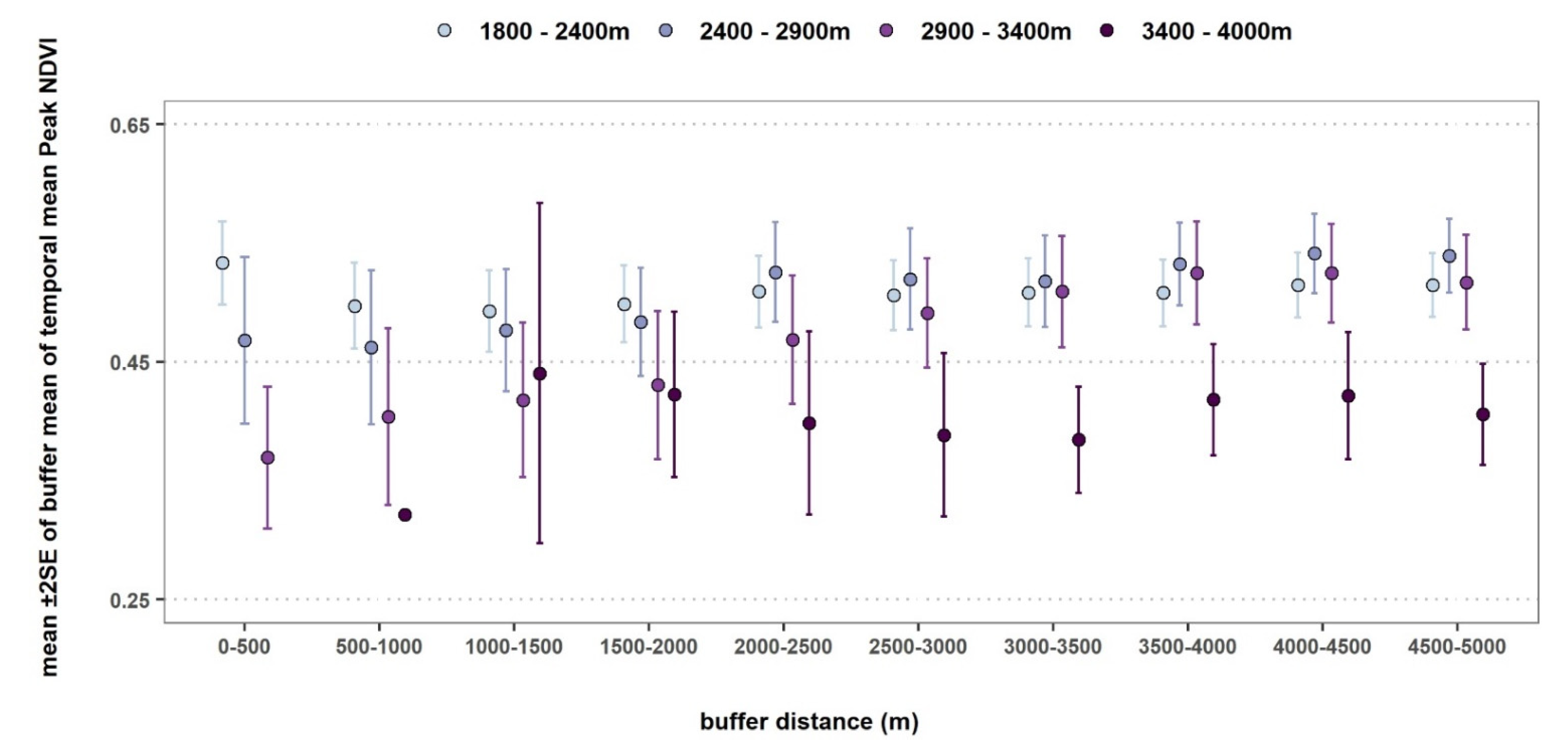
3.1. Buffer Mean Values of the Peak NDVI as a Function of Distance and Elevation

Figure 2 displays the spatial mean ±2SE values of the fitted NDVI Peak Height within each ring buffer calculated from the mean PH values across all years. Not surprisingly, there is considerable variation, but some patterns are evident. First, the PH decreased with increasing elevation. Second, the variation in the PH increased with elevation. Third, PH increased with distance from villages at 2400–2900 m and 2900–3400 m.

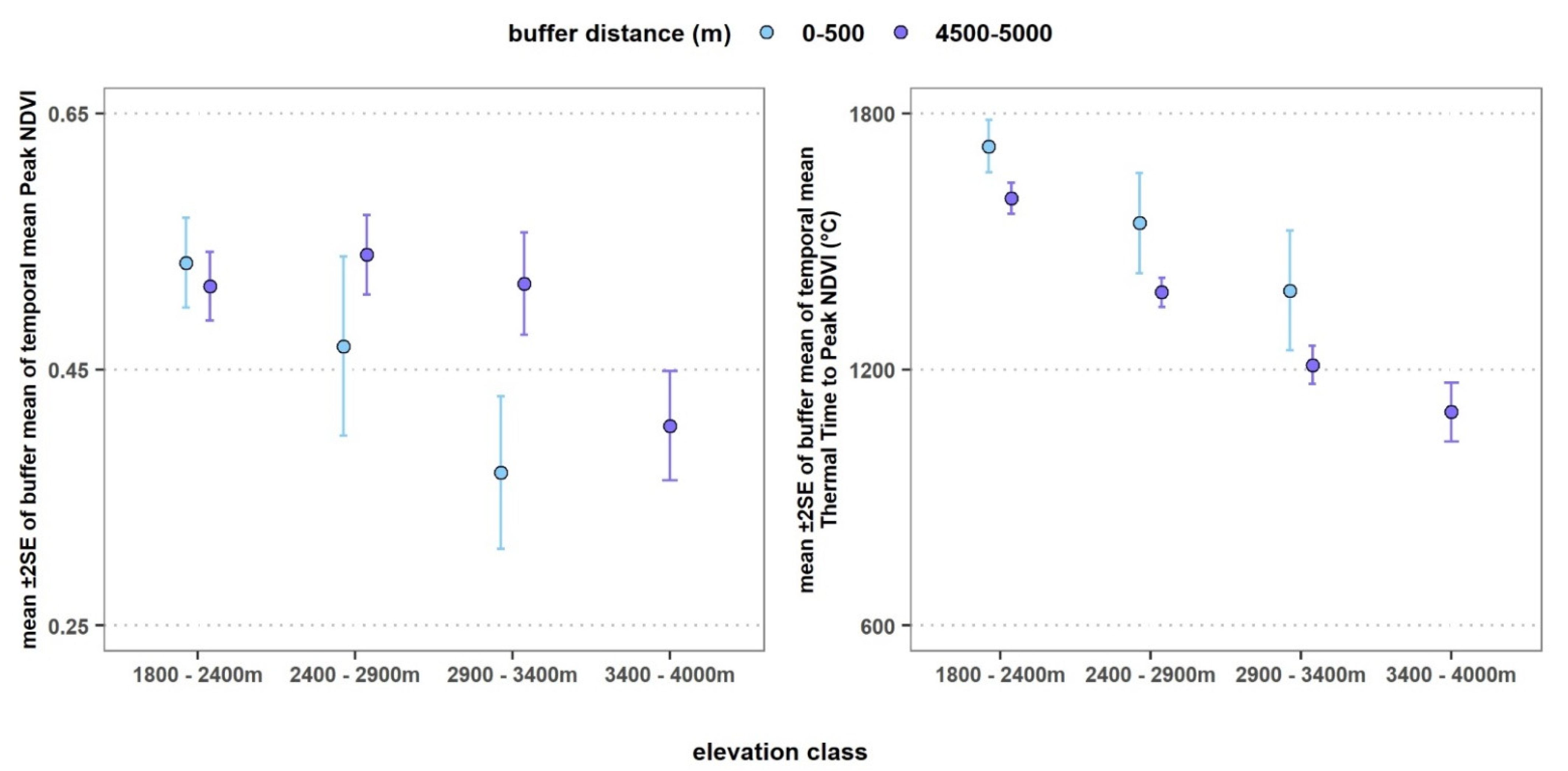
3.2. Contrasting Mean Values of Phenometrics Nearby and Far from Villages

Figure 3 subsets the distributions to focus on either end of the spatial series: the 0–500 m ring buffer captured those pasture areas closest to villages and the 4500–5000 m ring buffer captured pastures that were far from the focal village and not intruding on the ring buffer of another village. For PH (Figure 3, left panel), there was no difference in the lowest elevation class (1800–2400 m), but the differences between PH values nearby and far from villages were strong at both 2400–2900 m and 2900–3400 m, where the PH values in the distant ring buffer were higher than in the nearby ring buffer. However, the distributions of the mean PH values were significantly different between the 0–500 m and 4500–5000 m buffers only at the 2900–3400 m elevation range, according to the Kolmogorov–Smirnov two-sample test with the Dunn-Šidák correction for post-hoc multiple comparisons [41]. Note that in the highest elevation class (3400–4000 m), there were no pasture areas in the ring buffer nearest (0–500 m) to villages. It is also evident that the variation of PH in the nearby ring buffer appeared larger at higher elevations relative to that in the lowest elevation class, but this difference may result from fewer samples at high elevations.
The Thermal Time to Peak phenometric (Figure 3, right panel) decreased with elevation, as expected, and the distant TTP ring buffer means were consistently—but not significantly—lower than the nearby values.

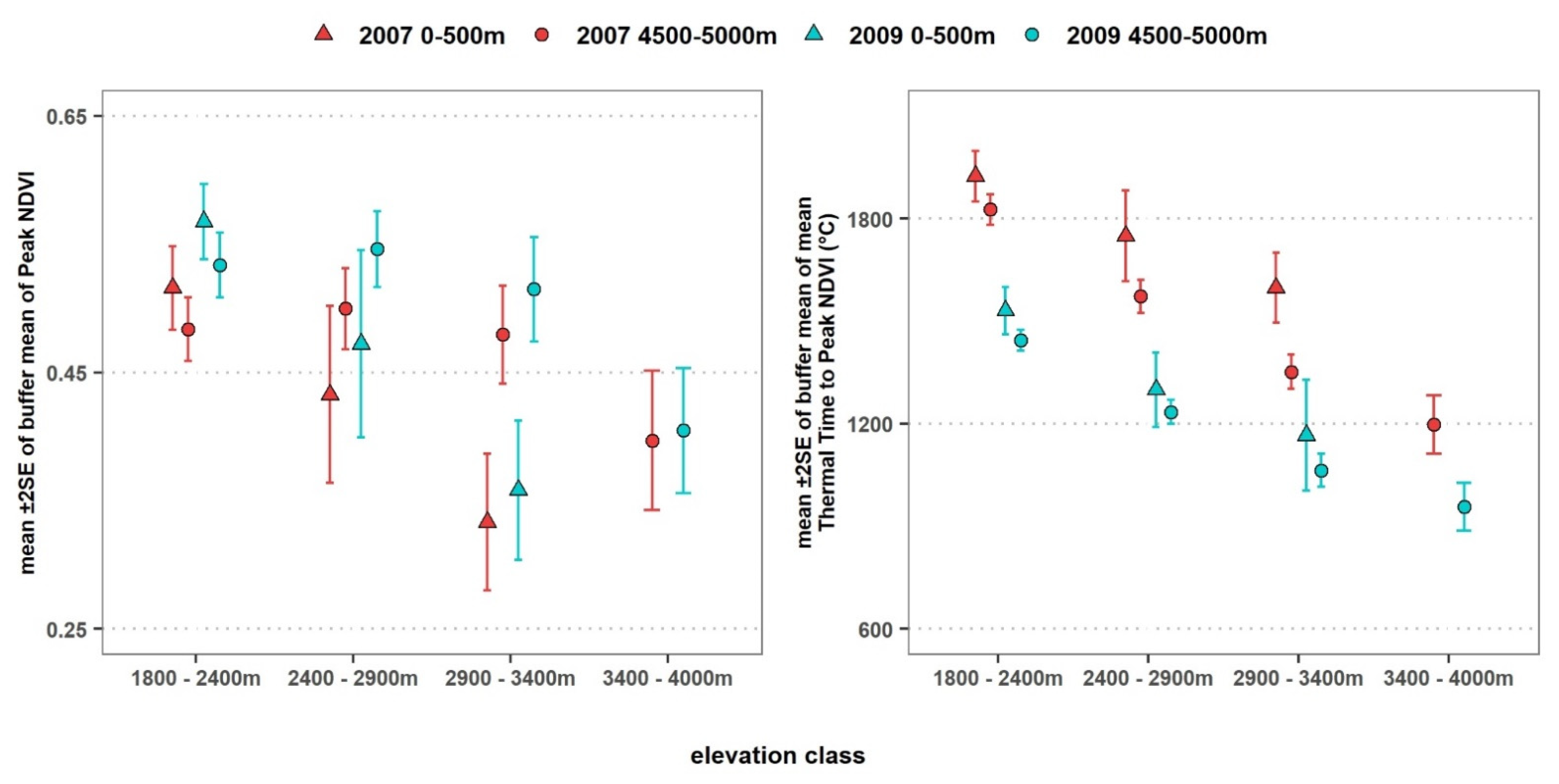
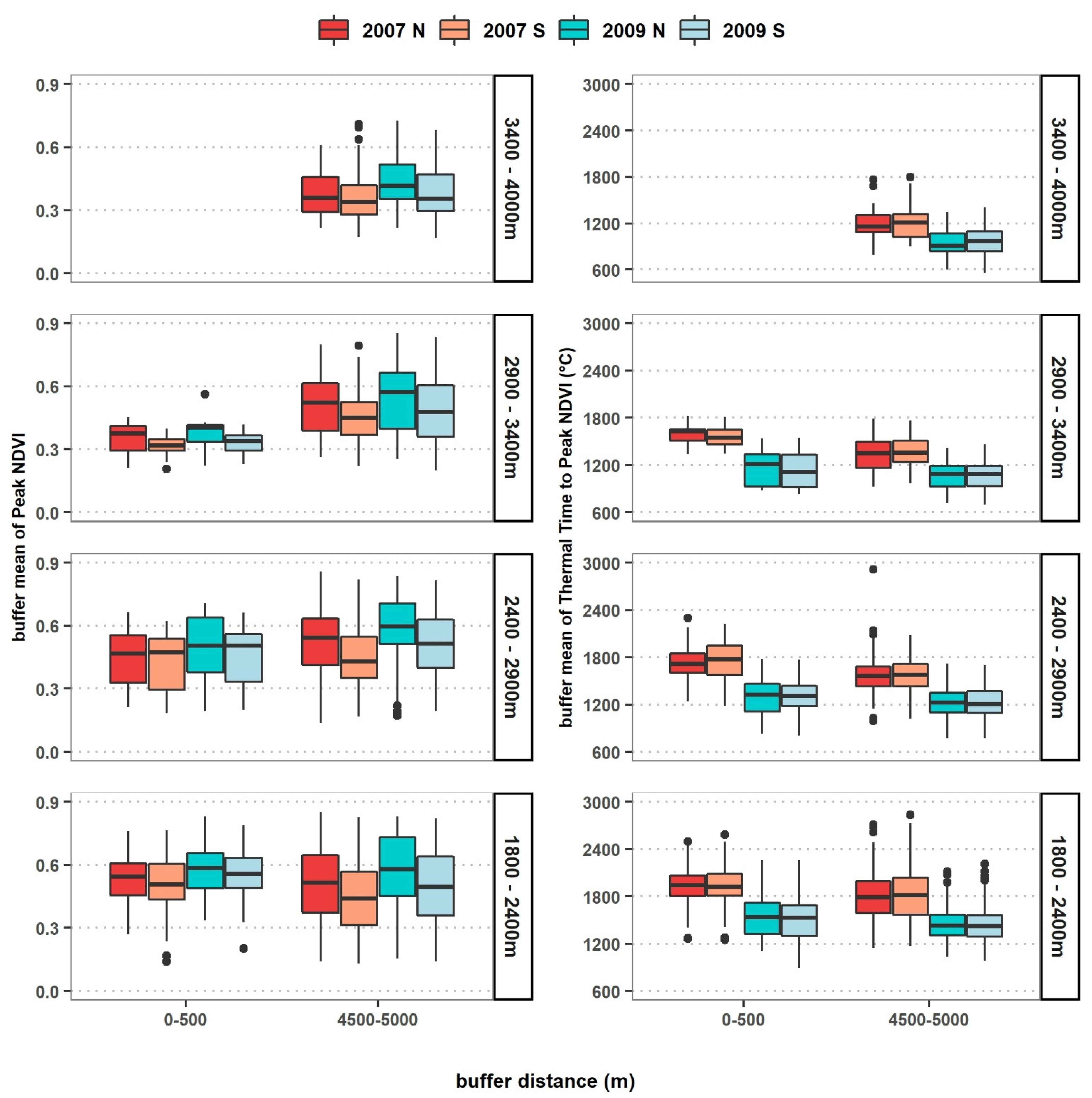
3.3. Influence of Weather on Phenometrics

Figure 4 shows the PH (left) and TTP (right) means for the ring buffers nearby versus far from the villages. For PH, the contrast between years and distance from villages was significant only for the 2900–3400 m elevation class (Figure 4, left). At the lowest elevation class, the nearby ring buffer means were not significantly different, but the distant means were. TTP was clearly lower during 2009, the wetter year, at all elevations, and lower at higher elevations, as expected. Evaluation by the Kolmogorov-Smirnov two-sample test (with the Dunn-Šidák correction) confirms what Figure 4 (right panel) shows: the TTP distributions were significantly different between 2007 and 2009 at every elevation class, but the difference between 0–500 m and 4500–5000 m ring buffer distributions was significant only at the 2900–3400 m elevation class and only in the drier year of 2007.

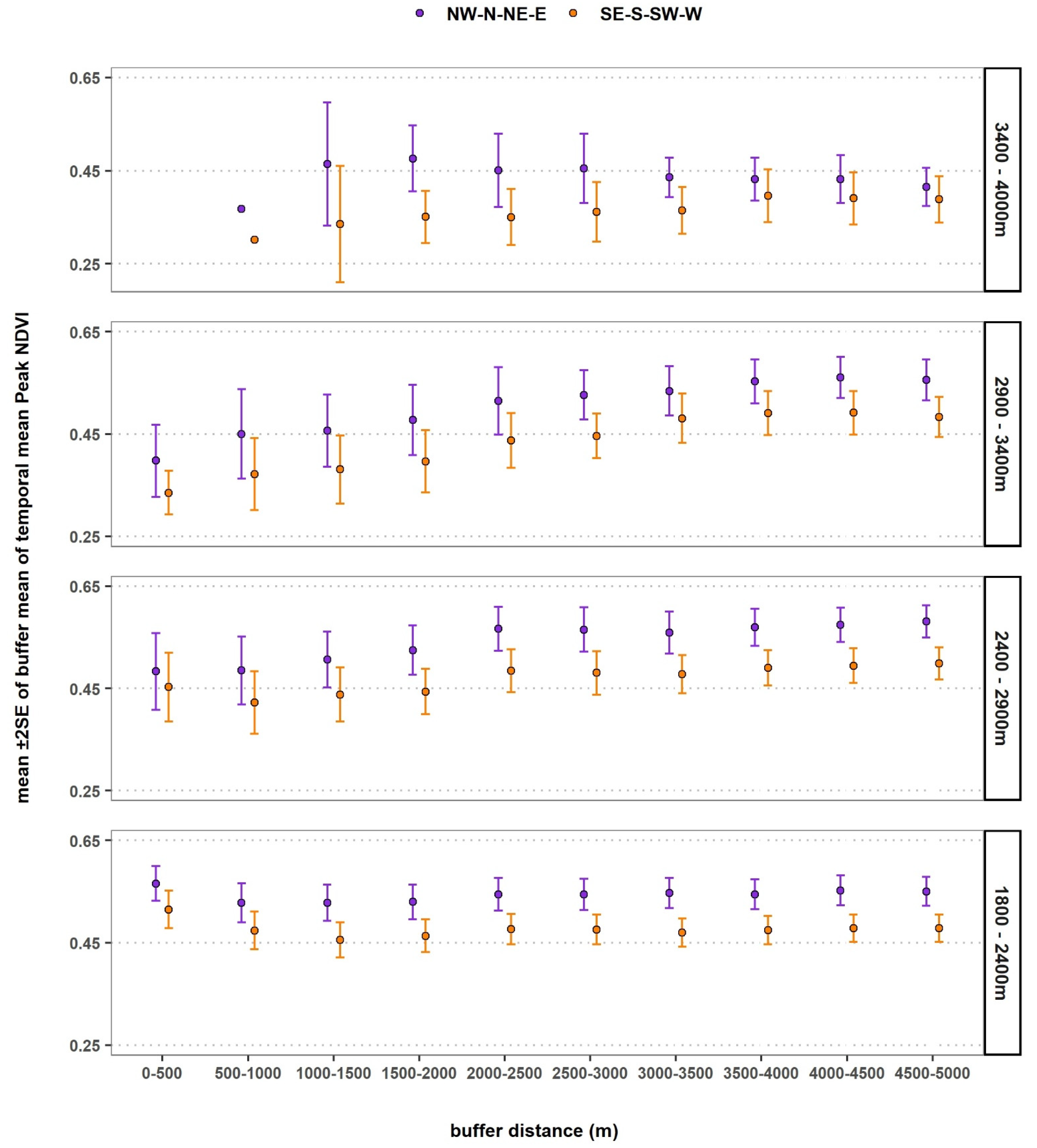
3.4. Influence of Aspect on Phenometrics

We tested for differences in the distributions of buffer means as a function of aspect (NW-N-NE-E vs. SE-S-SW-W) by distance from settlement point and elevation class using the Kolmogorov-Smirnov two-sample test with the Dunn-Šidák correction for post-hoc multiple comparisons. Northerly aspects consistently showed higher Peak Height means than in southerly aspects, but these differences were not statistically different at every distance or elevation class (Figure 5). In the lowest elevation class (1800–2400 m), the effect of aspect on PH was significant starting at the 2500–3000 m ring buffer; in the 2400–2900 m elevation class, the difference in PH between aspects appeared significant 500 m closer to the settlement point (i.e., at the 2000–2500 m ring buffer). In the two higher elevation classes, the aspect differences were not significant, but the variation about the means appears lower in the more distant ring buffers.

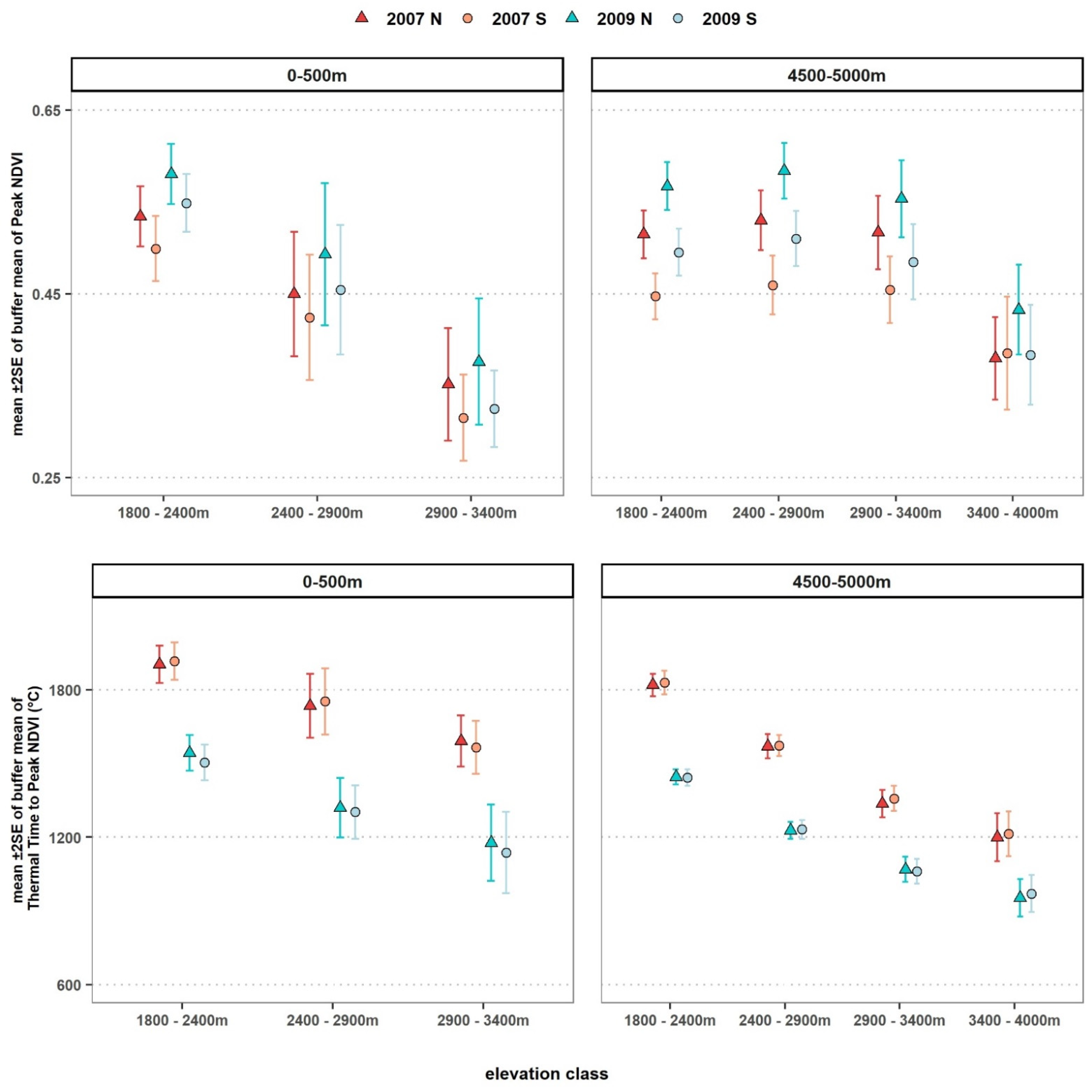
3.5. Interaction of Weather, Aspect, and Distance on Phenometrics

Figure 6 shows the distributions of phenometrics for northerly and southerly aspect slopes from pasture areas nearby (0–500 m) and far from (4500–5000 m) villages in the drier year of 2007 and the wetter year of 2009. The Kolmogorov-Smirnov two-sample test with the Dunn-Šidák correction reveals four patterns of interest in the Peak Height distributions: (1) the aspect effect on PH is significant at the two lower elevation classes only far from villages; (2) at the far ring buffer at each elevation class between 1800 m and 3400 m, the distributions of PH means from southerly aspects in the drier year of 2007 are significantly different from the northerly aspect PH means in the wetter year of 2009; (3) at each distance and elevation, distributions of PH means are not significantly different by year for the same aspect, i.e., the distributions of southerly (or northerly) aspect PH means are not different between years; and (4) the distributions of northerly aspect PH means in the drier year of 2007 are not significantly different from the southerly aspect PH means in the wetter year of 2009. This last pattern is clearer in Figure 7 (top panels) and illustrates how the northerly aspect slopes moderate the impact of dry years on pasture LSP.
The patterns in the TTP distributions were not surprising (Figure 6, right): (1) decreasing TTP with increasing elevation; (2) lower TTP values in the cooler, wetter year of 2009; and (3) no apparent aspect effect in the TTP buffer mean distributions. The bottom panels in Figure 7 show more clearly how strongly the TTP mean distributions diverge between years.

4. Discussion

The results of these linked analyses address the questions posed earlier. The Peak Height phenometric tends to increase in pasture areas as distance from the village increases. One interpretation of this pattern is the pasture areas near villages tend to be degraded. Winter pastures are closer to villages than either summer or transitional pastures and have been shown to exhibit significant differences in biogeochemistry and vegetation composition [5]. However, this general pattern can be modulated by the terrain, both elevation and aspect. Of the four elevation classes, significantly larger PH differences were seen between nearby and distant buffer rings in the 2900–3400 m elevation class (Figure 3, left). TTP decreased with elevation class but showed no clear difference between nearby and distant values (Figure 3, right), due in part to the much coarser spatial resolution of the LST data.
For the same reason, there was no clear influence of aspect on TTP (Figure 6, right panels; Figure 7, bottom panels). In contrast, the influence of aspect on PH was strongest in the lower elevation classes (Figure 5, bottom panels). When distant from a settlement, the PH on a northern aspect slope during a dry year appeared very similar to the PH on a southern aspect slope during a wet year (Figure 7, top right). However, in pasture areas closest to settlements, this aspect influence vanishes (Figure 7, top left).
The advantages of our study are several. First, we integrated long time series of two independent remote sensing products through a simple biometeorological model of land surface phenology that responds to the progress of growing season temperature rather than to the mere passing of days [37,38]. Second, the CxQ model has been shown to capture the initial seasonal peak well in grassland LSP [25,37,38]. Third, the finer spatial resolution of our analysis captured the influence of terrain features on vegetation growth and development as captured by the phenometrics [25].
Four limitations of our study are key. First, even the 30 m Landsat data can miss important landscape features influencing LSP [42]. Second, the 1 km spatial resolution of the MODIS LST product is coarser than would be optimal for use in rugged terrain. However, there are no effective alternatives at this point. Third, the CxQ model captures the initial seasonal peak but not necessarily the post-peak decay, particularly if there is heavy grazing post-peak [25]. This limitation is not as serious as it may first appear: we expect clear evidence of pasture degradation to appear only after several years of overgrazing, particularly if coupled with a severe drought. Fourth, while the pasture land-use mask was critical for omitting non-pastoral land-uses, there is substantial uncertainty associated with its development and accuracy. We have no accuracy assessment associated with it, and we expect that commission error is more likely than omission error, which would have the effect of increasing variance and decreasing the significance of the patterns. Finally, a key caveat for interpretation of these results should be noted: the 5 km extent of analysis was not meant to capture the summer pastures associated with villages. Summer pastures can be 10–50 km or more from a given village, and the spatial allocation and arrangement of summer pastures can be quite complicated.
Given our findings, to what extent do they raise questions about previous remote sensing studies on widespread degradation of pasture resources? The relationship between the scale of observation and the scale of the phenomenon of interest is crucial to the understanding and interpretability of the remote sensing data [43]. It is clear from these results that terrain effects can be obscured by coarser spatial resolution data, yet there is another scale to consider as well. Prior studies have demonstrated significant effects of climate oscillation modes on LSP in Central Asia [12,44,45]. However, more recent work at higher spatial resolution was not able to discern a significant influence from climate modes because the influence on LSP was overridden by local landscape structure [26].
Another facet of the degradation monitoring problem relates to the impact of spatial heterogeneity on the characterization of LSP. An important empirical study [46] explored how spatial heterogeneity in the land surface phenology observed at finer spatial resolution influences the timing of phenophase detection when observed at coarser spatial resolution. They found, when the land cover was homogeneous, that greater than 60% of Landsat 8 OLI 30 m pixels exhibiting start of season (SOS) detections were within 1 day of the SOS detection within a VIIRS pixel of 500 m spatial resolution. In contrast, less than 20% of the 30 m SOS detections were within 1 day if the land cover within the 500 m pixel was heterogeneous. They further reported that the SOS detection timing at the coarser spatial resolution was controlled by the timing when roughly 30% of the 30 m pixels within the 500 m pixel transitioned to SOS [46]. Thus, phenophase detections at coarser spatial resolutions are biased toward the earlier components in the vegetated land surface if the target landscape exhibits spatial heterogeneity. The study shows that the scaling effect on LSP is not resolvable with simple averaging. The mountain pastures of the Kyrgyz Republic and elsewhere in Central Asia exhibit a higher spatial heterogeneity than the croplands of central Iowa examined in [46]. Using a nonstandard MODIS product at 250 m spatial resolution, a study of pasture degradation in western Kyrgyz Republic found that pastures with a higher abundance of non-palatable vegetation exhibited later timing of peak NDVI during dry years in sub-alpine and mountain steppe ecozones but negligible impact in normal years [8]. The study is notable in that it included an extensive field component and demonstrated that higher NDVI values can accompany pasture degradation.
Several prior studies that have used MODIS data to detect trends in browning or greening in Kyrgyzstan and elsewhere in montane Central Asia may have been biased towards detecting browning trends and interpreting them as evidence of degradation due to using Collection 5 (C5) of the MODIS products. The differences between C5 and Collection 6 (C6 aka V006) are pronounced due to the loss of sensitivity of the red channel in the Terra MODIS [47,48]. Trend comparisons between the two collections have shown that significant negative trends in C5 were no longer significant in C6, and many nonsignificant trends in C5 appeared now as significant positive trends in C6 [49,50]. Two earlier studies [4,14] finding degradation in Kyrgyz pastures clearly used C5 products. Another study finding degradation [8] used data that was unlikely to have included the C6 corrections. A recent study [7] does not state which collection was used, but as the analysis period extended only until 2014, it is likely that it used C5 instead of C6 as well. The key point here is that as remote sensing products undergo upgrades that significantly change observed patterns, it is important to revisit those studies relying on earlier product versions to re-evaluate their findings in light of the new information.
A further concern is the use of simple linear slopes to detect significant trends. Applying ordinary least squares regression to a time series to fit a slope and declare the slope to be the trend has serious limitations from a statistical standpoint [51,52]. Positive autocorrelation reduces residual variance and inflates significance, increasing the risk of a Type I inferential error. Alternatives exist, such as the nonparametric Seasonal Kendall trend test, but it is not resistant to strong interannual autocorrelation. Fitting time series with autoregressive models has not been common in remote sensing studies.
Our findings suggest potential degradation in pasture areas as indicated by lower PHs closer to villages, but our analysis cannot rule out functional degradation arising from an increase in the coverage of nonpalatable species that can enhance NDVI without providing accessible forage [8,13,19]. Furthermore, what constitutes degradation in a particular socio-ecological system is frequently more subjective and culture-bound than is typically acknowledged [13,53,54,55].

5. Conclusions

We analyzed the landscape patterns of phenometrics based on fitted parameter coefficients of the land surface phenology model applied to 17 years of Landsat and MODIS seasonal time series across the montane pastures of the Kyrgyz Republic. We found that the Peak Height of NDVI generally decreased closer to villages, but the patterns were modulated—sometimes strongly—by elevation, aspect, and growing season weather. These findings raise questions about reports of pasture degradation based on coarser spatial resolution image time series. Our goal here was not to differentiate the relative contributions of these factors, because they are not susceptible to linear “unmixing”. Rather, we sought to recognize their potential influence on the mixed signal observed at coarser spatial resolutions and to urge caution in interpreting, for instance, declines in NDVI trends with pasture degradation and increases with pasture remediation. The situation is more complicated. Due to the spatial heterogeneous distribution of pastures and pasture usage in mountainous landscapes, contextual information should be used to interpret remotely sensed patterns and trends in an appropriately nuanced manner.

Author Contributions

Conceptualization, G.M.H. and M.A.T.; methodology, G.M.H. and M.A.T.; software, M.A.T.; resources, G.M.H.; data curation, M.A.T.; writing—original draft preparation, G.M.H. and M.A.T.; writing—review, editing, and revision, G.M.H. and M.A.T.; visualization, M.A.T.; supervision, G.M.H.; project administration, G.M.H.; funding acquisition, G.M.H. Both authors have read and agreed to the published version of the manuscript.

Funding

This research was funded by the NASA LCLUC program, grant number 80NSSC20K0411. The APC was funded by the same grant.

Data Availability Statement

Part of the data used in this work were supplied from our previous work [25] and can be found in the NASA Land Use/Land Cover project repository: https://lcluc.umd.edu/metadatafiles/LCLUC-2015-PI-Henebry/RSE/, accessed on 20 June 2021. The remaining data presented in this study are available on request from the corresponding author ([email protected]).

Acknowledgments

We appreciate the assistance and data sharing from Kamilya Kelgenbaeva. We also appreciate discussions with Munavar Zhumanova about pasture degradation. We would like to thank all reviewers and editors for their time and effort to improve the clarity, precision, and relevance of this publication.

Conflicts of Interest

The authors declare no conflict of interest.

References

  1. FAOStats: Statistics page of the Food and Agriculture Organization (FAO). Available online: http://www.fao.org/faostat/en/#data/RL (accessed on 20 June 2021).
  2. Akimaliev, D.A.; Zaurov, D.E.; Eisenman, S.W. The geography, climate and vegetation of Kyrgyzstan. In Medicinal Plants of Central Asia: Uzbekistan and Kyrgyzstan; Springer: New York, NY, USA, 2013; pp. 1–4. [Google Scholar]
  3. Borchardt, P.; Schickhoff, U.; Scheitweiler, S.; Kulikov, M. Mountain pastures and grasslands in the SW Tien Shan, Kyrgyzstan—Floristic patterns, environmental gradients, phytogeography, and grazing impact. J. Mt. Sci. 2011, 8, 363–373. [Google Scholar] [CrossRef]
  4. Dubovyk, O.; Landmann, T.; Dietz, A.; Menz, G. Quantifying the impacts of environmental factors on vegetation dynamics over climatic and management gradients of Central Asia. Remote Sens. 2016, 8, 600. [Google Scholar] [CrossRef] [Green Version]
  5. Hoppe, F.; Kyzy, T.Z.; Usupbaev, A.; Schickhoff, U. Rangeland degradation assessment in Kyrgyzstan: Vegetation and soils as indicators of grazing pressure in Naryn Oblast. J. Mt. Sci. 2016, 13, 1567–1583. [Google Scholar] [CrossRef]
  6. Kulikov, M.; Schickhoff, U.; Borchardt, P. Spatial and seasonal dynamics of soil loss ratio in mountain rangelands of south-western Kyrgyzstan. J. Mt. Sci. 2016, 13, 316–329. [Google Scholar] [CrossRef]
  7. Wang, Y.; Yue, H.; Peng, Q.; He, C.; Hong, S.; Bryan, B.A. Recent responses of grassland net primary productivity to climatic and anthropogenic factors in Kyrgyzstan. Land Degrad. Dev. 2020, 31, 2490–2506. [Google Scholar] [CrossRef]
  8. Zhumanova, M.; Mönnig, C.; Hergarten, C.; Darr, D.; Wrage-Mönnig, N. Assessment of vegetation degradation in mountainous pastures of the Western Tien-Shan, Kyrgyzstan, using eMODIS NDVI. Ecol. Indic. 2018, 95, 527–543. [Google Scholar] [CrossRef]
  9. Kerven, C.; Steimann, B.; Dear, C.; Ashley, L. Researching the future of pastoralism in Central Asia’s mountains: Examining development orthodoxies. Mt. Res. Dev. 2012, 32, 368–377. [Google Scholar] [CrossRef] [Green Version]
  10. Robinson, S. Land degradation in Central Asia: Evidence, Perception and Policy. In The End of Desertification? Behnke, R., Mortimore, M., Eds.; Springer: Heidelberg, Germany, 2016; pp. 451–490. [Google Scholar] [CrossRef]
  11. de Beurs, K.M.; Henebry, G.; Owsley, B.C.; Sokolik, I. Using multiple remote sensing perspectives to identify and attribute land surface dynamics in Central Asia 2001–2013. Remote Sens. Environ. 2015, 170, 48–61. [Google Scholar] [CrossRef]
  12. de Beurs, K.M.; Henebry, G.; Owsley, B.C.; Sokolik, I.N. Large scale climate oscillation impacts on temperature, precipitation and land surface phenology in Central Asia. Environ. Res. Lett. 2018, 13, 065018. [Google Scholar] [CrossRef]
  13. Eddy, I.M.; Gergel, S.E.; Coops, N.C.; Henebry, G.; Levine, J.; Zerriffi, H.; Shibkov, E. Integrating remote sensing and local ecological knowledge to monitor rangeland dynamics. Ecol. Indic. 2017, 82, 106–116. [Google Scholar] [CrossRef]
  14. Kulikov, M.; Schickhoff, U. Vegetation and climate interaction patterns in Kyrgyzstan: Spatial discretization based on time series analysis. Erdkunde 2017, 71, 143–165. [Google Scholar] [CrossRef]
  15. Xu, H.-J.; Wang, X.-P.; Zhang, X.-X. Decreased vegetation growth in response to summer drought in Central Asia from 2000 to 2012. Int. J. Appl. Earth Obs. Geoinf. 2016, 52, 390–402. [Google Scholar] [CrossRef]
  16. Xu, H.-J.; Wang, X.-P.; Yang, T.-B. Trend shifts in satellite-derived vegetation growth in Central Eurasia, 1982–2013. Sci. Total Environ. 2017, 579, 1658–1674. [Google Scholar] [CrossRef] [PubMed]
  17. Imanberdieva, N. Flora and plant formations distributed in At-Bashy Valleys–Internal Tien Shan in Kyrgyzstan and interactions with climate. In Climate Change Impacts on High-Altitude Ecosystems; Öztürk, M., Hakeem, K.R., Faridah-Hanum, I., Efe, R., Eds.; Springer: New York, NY, USA, 2015; pp. 569–590. ISBN 9783319128597. [Google Scholar]
  18. Nowak, A.; Świerszcz, S.; Nowak, S.; Nobis, M. Classification of tall-forb vegetation in the Pamir-Alai and western Tian Shan Mountains (Tajikistan and Kyrgyzstan, Middle Asia). Veg. Classif. Surv. 2020, 1, 191–217. [Google Scholar] [CrossRef]
  19. Zhumanova, M.; Wrage-Mönnig, N.; Jurasinski, G. Long-term vegetation change in the Western Tien-Shan Mountain pastures, Central Asia, driven by a combination of changing precipitation patterns and grazing pressure. Sci. Total Environ. 2021, 781, 146720. [Google Scholar] [CrossRef] [PubMed]
  20. de Beurs, K.M.; Wright, C.K.; Henebry, G. Dual scale trend analysis for evaluating climatic and anthropogenic effects on the vegetated land surface in Russia and Kazakhstan. Environ. Res. Lett. 2009, 4, 045012. [Google Scholar] [CrossRef]
  21. Groisman, P.; Bulygina, O.; Henebry, G.; Speranskaya, N.; Shiklomanov, A.; Chen, Y.; Tchebakova, N.; Parfenova, E.; Tilinina, N.; Zolina, O.; et al. Dryland belt of Northern Eurasia: Contemporary environmental changes and their consequences. Environ. Res. Lett. 2018, 13, 115008. [Google Scholar] [CrossRef]
  22. Li, Z.; Chen, Y.; Li, W.; Deng, H.; Fang, G. Potential impacts of climate change on vegetation dynamics in Central Asia. J. Geophys. Res. Atmos. 2015, 120, 12345–12356. [Google Scholar] [CrossRef]
  23. Tomaszewska, M.A.; Henebry, G. Changing snow seasonality in the highlands of Kyrgyzstan. Environ. Res. Lett. 2018, 13, 065006. [Google Scholar] [CrossRef]
  24. Xenarios, S.; Gafurov, A.; Schmidt-Vogt, D.; Sehring, J.; Manandhar, S.; Hergarten, C.; Shigaeva, J.; Foggin, M. Climate change and adaptation of mountain societies in Central Asia: Uncertainties, knowledge gaps, and data constraints. Reg. Environ. Chang. 2019, 19, 1339–1352. [Google Scholar] [CrossRef]
  25. Tomaszewska, M.A.; Nguyen, L.H.; Henebry, G. Land surface phenology in the highland pastures of montane Central Asia: Interactions with snow cover seasonality and terrain characteristics. Remote Sens. Environ. 2020, 240, 111675. [Google Scholar] [CrossRef]
  26. Tomaszewska, M.A.; Henebry, G.M. How much variation in land surface phenology can climate oscillation modes explain at the scale of mountain pastures in Kyrgyzstan? Int. J. Appl. Earth Obs. Geoinf. 2020, 87, 102053. [Google Scholar] [CrossRef]
  27. Azykova, E.K. Geographyical and landscape characteristics of mountain territories. In Mountains of Kyrgyzstan; Aidaraliev, A.A., Ed.; Technology: Bishkek, Kyrgyzstan, 2002. [Google Scholar]
  28. Asian Development Bank. Central Asia Atlas of Natural Resource; Central Asian Countries Initiative for Land Management and Asian Development Bank: Manila, Philippines, 2010. [Google Scholar]
  29. Asian Development Bank. Central Asian Countries Initiative for Land Management (CACILM) Multicountry Partnership Framework Support Project. Available online: https://www.adb.org/projects/38464-012/main (accessed on 20 June 2021).
  30. NASA JPL. NASA Shuttle Radar Topography Mission Global 1 Arc Second. 2013. Available online: https://lpdaac.usgs.gov/products/srtmgl1v003/ (accessed on 20 June 2021). [CrossRef]
  31. Wan, Z.; Hook, S.; Hulley, G. MOD11A2 MODIS/Terra Land Surface Temperature/Emissivity 8-Day L3 Global 1 km SIN Grid V006; NASA EOSDIS Land Processes DAAC: Sioux Falls, SD, USA, 2015. [Google Scholar]
  32. Roy, D.; Kovalskyy, V.; Zhang, H.; Vermote, E.; Yan, L.; Kumar, S.S.; Egorov, A. Characterization of Landsat-7 to Landsat-8 reflective wavelength and normalized difference vegetation index continuity. Remote Sens. Environ. 2016, 185, 57–70. [Google Scholar] [CrossRef] [Green Version]
  33. Fisher, J.I.; Mustard, J.F.; Vadeboncoeur, M. Green leaf phenology at Landsat resolution: Scaling from the field to the satellite. Remote Sens. Environ. 2006, 100, 265–279. [Google Scholar] [CrossRef]
  34. Melaas, E.; Friedl, M.A.; Zhu, Z. Detecting interannual variation in deciduous broadleaf forest phenology using Landsat TM/ETM+ data. Remote Sens. Environ. 2013, 132, 176–185. [Google Scholar] [CrossRef]
  35. Pereladova, O.; Krever, V.; Shestakov, A. ECONET—Web for Life; Central Asia: Moscow, Russia, 2006. [Google Scholar]
  36. de Beurs, K.M.; Henebry, G. Land surface phenology, climatic variation, and institutional change: Analyzing agricultural land cover change in Kazakhstan. Remote Sens. Environ. 2004, 89, 497–509. [Google Scholar] [CrossRef]
  37. Henebry, G.M.; de Beurs, K.M. Remote sensing of land surface phenology: A prospectus. In Phenology: An Integrative Environmental Science; Schwartz, M.D., Ed.; Springer Netherlands: Dordrecht, The Netherlands, 2013; Volume 9789400769, pp. 385–411. ISBN 9789400769250. [Google Scholar]
  38. de Beurs, K.M.; Henebry, G.M. Spatio-temporal statistical methods for modelling land surface phenology. In Phenological Research: Methods for Environmental and Climate Change Analysis; Hudson, I.L., Keatley, M.R., Eds.; Springer: Dordrecht, The Netherlands, 2010; pp. 177–208. ISBN 978-90-481-3334-5. [Google Scholar]
  39. Moritz, S.; Bartz-Beielstein, T. imputeTS: Time Series Missing Value Imputation in R. R J. 2017, 9, 207. [Google Scholar] [CrossRef] [Green Version]
  40. Goodin, D.G.; Henebry, G. A technique for monitoring ecological disturbance in tallgrass prairie using seasonal NDVI trajectories and a discriminant function mixture model. Remote Sens. Environ. 1997, 61, 270–278. [Google Scholar] [CrossRef]
  41. Šidák, Z. Rectangular confidence regions for the means of multivariate normal distributions. J. Am. Stat. Assoc. 1967, 62, 626–633. [Google Scholar] [CrossRef]
  42. Cheng, Y.; Vrieling, A.; Fava, F.; Meroni, M.; Marshall, M.; Gachoki, S. Phenology of short vegetation cycles in a Kenyan rangeland from PlanetScope and Sentinel-2. Remote Sens. Environ. 2020, 248, 112004. [Google Scholar] [CrossRef]
  43. Strahler, A.H.; Woodcock, C.E.; Smith, J.A. On the nature of models in remote sensing. Remote Sens. Environ. 1986, 20, 121–139. [Google Scholar] [CrossRef]
  44. de Beurs, K.M.; Henebry, G. Northern annular mode effects on the land surface phenologies of Northern Eurasia. J. Clim. 2008, 21, 4257–4279. [Google Scholar] [CrossRef]
  45. Wright, C.K.; de Beurs, K.M.; Henebry, G. Land surface anomalies preceding the 2010 Russian heat wave and a link to the North Atlantic oscillation. Environ. Res. Lett. 2014, 9, 124015. [Google Scholar] [CrossRef]
  46. Zhang, X.; Wang, J.; Gao, F.; Liu, Y.; Schaaf, C.; Friedl, M.; Yu, Y.; Jayavelu, S.; Gray, J.; Liu, L.; et al. Exploration of scaling effects on coarse resolution land surface phenology. Remote Sens. Environ. 2017, 190, 318–330. [Google Scholar] [CrossRef] [Green Version]
  47. Wang, D.; Morton, D.; Masek, J.; Wu, A.; Nagol, J.; Xiong, X.; Levy, R.; Vermote, E.; Wolfe, R. Impact of sensor degradation on the MODIS NDVI time series. Remote Sens. Environ. 2012, 119, 55–61. [Google Scholar] [CrossRef] [Green Version]
  48. Lyapustin, A.; Wang, Y.; Xiong, X.; Meister, G.; Platnick, S.; Levy, R.; Franz, B.; Korkin, S.; Hilker, T.; Tucker, J.; et al. Scientific impact of MODIS C5 calibration degradation and C6+ improvements. Atmos. Meas. Tech. 2014, 7, 4353–4365. [Google Scholar] [CrossRef] [Green Version]
  49. Zhang, Y.; Song, C.; Band, L.E.; Sun, G.; Li, J. Reanalysis of global terrestrial vegetation trends from MODIS products: Browning or greening? Remote Sens. Environ. 2017, 191, 145–155. [Google Scholar] [CrossRef] [Green Version]
  50. Heck, E.; de Beurs, K.M.; Owsley, B.C.; Henebry, G.M. Evaluation of the MODIS collections 5 and 6 for change analysis of vegetation and land surface temperature dynamics in North and South America. ISPRS J. Photogramm. Remote Sens. 2019, 156, 121–134. [Google Scholar] [CrossRef]
  51. de Beurs, K.; Henebry, G. Trend analysis of the Pathfinder AVHRR Land (PAL) NDVI data for the deserts of Central Asia. IEEE Geosci. Remote Sens. Lett. 2004, 1, 282–286. [Google Scholar] [CrossRef]
  52. de Beurs, K.M.; Henebry, G. A statistical framework for the analysis of long image time series. Int. J. Remote Sens. 2005, 26, 1551–1573. [Google Scholar] [CrossRef]
  53. Levine, J.; Isaeva, A.; Eddy, I.; Foggin, M.; Gergel, S.; Hagerman, S.; Zerriffi, H. A cognitive approach to the post-Soviet Central Asian pasture puzzle: New data from Kyrgyzstan. Reg. Environ. Chang. 2017, 17, 941–947. [Google Scholar] [CrossRef]
  54. Levine, J.; Isaeva, A.; Zerriffi, H.; Eddy, I.M.S.; Foggin, M.; Gergel, S.E.; Hagerman, S.M. Testing for consensus on Kyrgyz rangelands: Local perceptions in Naryn oblast. Ecol. Soc. 2019, 24, 36. [Google Scholar] [CrossRef]
  55. Liechti, K. The meanings of pasture in resource degradation negotiations: Evidence from post-socialist rural Kyrgyzstan. Mt. Res. Dev. 2012, 32, 304–312. [Google Scholar] [CrossRef] [Green Version]
Figure 1. Pasture land use area (light tan) and selected settlement points (blue-green) in the Kyrgyz Republic (from [28,29]) draped over the SRTM 30 m DEM [30] (Projected coordinate system: Albers Conic Equal Area). Province (oblast) names appear in yellow.
Remotesensing 13 03449 g001
Figure 2. Elevational gradients in modeled peak NDVI: mean ±2SE of the ten ring buffer mean values calculated from the temporal mean Peak Height. Sequential color scheme starting from left represents four classes of elevation: 1800–2400 m, 2400–2900 m, 2900–3400 m, and 3400–4000 m.
Remotesensing 13 03449 g002
Figure 3. Contrasting values from pasture areas nearby and far from villages: mean ±2SE of the two (0–500 m in light blue, 4500–5000 m in purple) buffer mean values of temporal mean Peak Height (left) and mean Thermal Time to Peak (right) for the four elevation classes.
Remotesensing 13 03449 g003
Figure 4. Differences in phenometric values (Peak Height at left, and Thermal Time to Peak at right) arising from distance and weather: mean ±2SE of the two ring buffer (0–500 m as a triangle, 4500–5000 m as a circle) means of 2007 (in red) and 2009 (in dark cyan) for the four elevation classes.
Remotesensing 13 03449 g004
Figure 5. Contrasting values from pasture aspect: mean ±2SE of the ten ring buffer mean values of temporal mean Peak Height at two contrasting aspects (northern aspects in dark purple; southern aspects in dark orange) for the four elevation classes.
Remotesensing 13 03449 g005
Figure 6. Interaction of weather, aspect, and distance: distributions of the phenometrics (Peak Height (left) and Thermal Time to Peak (right) from two nearby (0–500 m) and distant (4500–5000 m) ring buffer mean values calculated from the hotter, drier year of 2007 (northern aspects [N] in red, southern aspects [S] in orange) and the cooler, wetter year of 2009 (northern aspects [N] in a dark cyan, southern aspects [S] in a light blue)) at the four elevation classes.
Remotesensing 13 03449 g006
Figure 7. Differences in phenometric values (Peak Height on top and Thermal Time to Peak at bottom) arising from contrasts in weather and aspect: mean ±2SE of the two ring buffers at 0–500 m (left) and 4500–5000 m (right) from villages for hotter, drier 2007 (northern aspects [N] in a red triangle, southern aspects [S] in an orange circle) and cooler, wetter 2009 (northern aspects [N] in a dark cyan triangle, southern aspects [S] in a light blue circle) for the four elevation classes.
Remotesensing 13 03449 g007
Table 1. Number of settlement points after dataset revision and filtering per province (oblast).
Province (Oblast)Total PointsPoints after 10 km Filter
Batken6336
Chuy6733
Issyk-Kul10045
Jalal-Abad11358
Naryn9644
Osh13756
Talas4121
TOTAL617293
Publisher’s Note: MDPI stays neutral with regard to jurisdictional claims in published maps and institutional affiliations.

