
Semi-Supervised Convolutional Long Short-Term Memory Neural Networks for Time Series Land Cover Classification


1
School of Geosciences and Info-Physics, Central South University, Changsha 410083, China
2
State Key Laboratory of Resources and Environment Information System, Institute of Geographical Science and Natural Resources, Chinese Academy of Sciences, Beijing 100101, China
*
Author to whom correspondence should be addressed.
Remote Sens. 2021, 13(17), 3504; https://0-doi-org.brum.beds.ac.uk/10.3390/rs13173504
Submission received: 10 July 2021
/
Revised: 30 August 2021
/
Accepted: 30 August 2021
/
Published: 3 September 2021
(This article belongs to the Section Earth Observation Data)
Abstract
:Time series images with temporal features are beneficial to improve the classification accuracy. For abstract temporal and spatial contextual information, deep neural networks have become an effective method. However, there is usually a lack of sufficient samples in network training: one is the loss of images or the discontinuous distribution of time series data because of the inevitable cloud cover, and the other is the lack of known labeled data. In this paper, we proposed a Semi-supervised convolutional Long Short-Term Memory neural network (SemiLSTM) for time series remote sensing images, which was validated on three data sets with different time distributions. It achieves an accurate and automated land cover classification via a small number of labeled samples and a large number of unlabeled samples. Besides, it is a robust classification algorithm for time series optical images with cloud coverage, which reduces the requirements for cloudless remote sensing images and can be widely used in areas that are often obscured by clouds, such as subtropical areas. In conclusion, this method makes full advantage of spectral-spatial-temporal characteristics under the condition of limited training samples, especially expanding time context information to enhance classification accuracy.
1. Introduction
Remote sensing image classification is widely used in various areas of research and application, such as change detection, geography national condition monitoring, and global ecological environment changes [1,2,3,4,5,6]. With the growing development of remote sensing technology, the types and quantities of remotely sensed data have soared. It has become easier to access multi-source and multi-temporal Earth Observation (EO) data. The increasing demand for products encourages an increasing number of scholars to research a novel approach aimed at improving the accuracy of classification and meeting a wide range of information requirements and applications.
The current classification methods are mainly based on the classification tasks of singe-phase image. It can be roughly divided into unsupervised, supervised, and semi-supervised classification methods. Unsupervised classification algorithms cluster elements by similar attributes without any prior knowledge, like K-means and ISODATA [7]. But they are hard to interpret and are time consuming for high dimension or enormous volume of data [8]. On the contrary, supervised classification algorithms identify other unknown categories of pixels by learning prior human intervention (e.g., Decision Trees, DT [9]; Random Forests, RF [10]; Support Vector Machines, SVM [11]; and Artificial Neural Networks, ANN [12]). For these, selecting a representative and abundant training samples is crucial. However, the training samples are artificially selected through limited experience and knowledge whether it is field exploration or reference data. There is no guarantee that the selected classification samples have a valid representation of corresponding land cover classes. Therefore, semi-supervised learning from the field of data mining applies to various classifiers, like transductive SVM [13], the self-learning method [14,15], and the graph-based method [16]. It mines the inherent structural features of object types in unlabeled samples to correct fitting classifiers that may be caused by the poor representation of labeled samples. The semi-supervised classification methods can improve the problem of poor representative known samples and limited effective training samples in practice.
With the development of satellite technologies, the accumulation of multi-source and historical remote sensing images enables more abundant information to be exploited, not limited to a single-phase image. It turns out that inclusion of time and multi-angle ancillary data can improve the accuracy of the classification [17]. As a result, time series satellite data has been widely used in classification and other fields. Different features in time context are conducive to accurately distinguish various ground objects. For example, the time series NDVI was used to mine phenological features, which can significantly improve the classification accuracy [18].
With the heavy attention on deep learning, numerous studies have investigated that the deep neural networks can effectively and automatically extract abstract feature representations from temporal data. In particular, Recurrent Neural Networks (RNNs) have been widely employed in time series analysis and applications owing to their outstanding performance in complex temporal correlations. When an image is divided into sequence data by row, LSTM can implement a high-precision classification result [19]. Then, LSTM was used to model temporal vegetation and identify various crops in [20]. They also proved that the LSTM-based classifier performed better than other methods (the classical RNN and the SVM baseline). In addition, Convolutional Neural Networks (CNNs) have achieved a high accuracy of semantic segmentation and classification in remote sensing imagery due to the spatial autocorrelation [21,22]. On this basis, some trainable network variants were proposed which combines the strengths of both convolutional and recurrent neural network components. Convolutional LSTM network (ConvLSTM) was first proposed to the spatiotemporal sequence precipitation nowcasting [23]. After that, a Recurrent Convolutional Neural Network (ReCNN) was utilized for change detection in biphasic multispectral images [24].
However, deep neural networks usually require the quantity and quality of training samples, which undoubtedly increases the workload and computation [25]. On the one hand, the selection of training samples is a major challenge. In terms of the problem of sample representation in the above-mentioned supervised classification, people default that the selected samples have a good representation for individual category because of the subjective judgment. It is not conductive to the further development of image classification methods, because the unsatisfactory classification results are always attributed to the inapplicability of the algorithm or the parameter selection. On the other hand, the features of ground objects that change over time are more complex. It is common for many types of changes to occur simultaneously in the same area during the monitoring period, especially in a long time period. The change types can be roughly divided into two types. One is that the properties of the target objects change. For example, in urban construction, the original cultivated land or unused land may gradually become construction land. The other is a “pseudo-change” in which the properties of the target object remain unchanged. This change is usually the natural growth change of plants, like wheat. The image spectral reflectance of wheat is different during the phenological period of emergence, heading, flowering, and maturity. In order to ensure the classification accuracy of time series images with various types of changes, more adequate prior knowledge is needed for training. But in fact, it is easier to get a label at a certain moment instead of multiple or all labels. If a large amount of training labels is required, there will be a lot of labor costs.
Besides, for optical remote sensing images, it is difficult to avoid cloud, snow, and shadow coverage. Even though historical satellite images are easy to seek, there are still missing images or discontinuous time series data because of these noisy observations. This problem will affect accuracy of target recognition and classification, so a sort of preprocessing will be employed in advance, such as cloud and cloud shadow detection [26] or fitting the multi-temporal curve to the missing data problem [27,28].
In order to address these problems mentioned above, we propose a SemiLSTM for time series land cover classification. The major contributions of this work are as follows: (i) It achieves an excellent classification via a small group of labeled samples in time series data; (ii) it is a robust classification model for time series optical remote sensing data with the influence of noise (especially clouds and shadows), which decreases the requirements for time series images without clouds and can be widely used in areas that are often obscured by clouds, such as subtropical areas; (iii) it makes full use of spectral-spatial-temporal characteristics, especially expanding the time context information to enhance classification accuracy.
In previous work, we have experimented with recurrent networks on time series data with similar time resolution, and achieved promising results [29]. Based on this, we revised a more reasonable training mode and conducted experiments on three data sets with different time distributions.
The remainder of this paper is organized as follows: Section 2 describes the architecture and working principle of our proposed SemiLSTM method, and other classifiers for comparison. Then, the experimental data sets, experimental setup, and results are presented in Section 3 and Section 4. Section 5 discusses the length of temporal context, the appropriate number of labeled training samples and the robustness for time series land cover classification with different cloud coverage. The final Section 6 concludes the paper.
2. Methodology
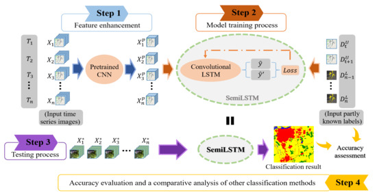
In this study, we designed a SemiLSTM for classification of long time series images. It uses a small number of labeled samples and a large number of unlabeled samples to extract the spectral, spatial, and temporal information. Figure 1 reveals the basic framework of the proposed SemiLSTM method, which can be decomposed into two parts: the pretrained model and the semi-supervised spatiotemporal modeling. In the following, we first describe how to use a trained CNN model on all images to enhance spatial features. Then, we detail how the convolutional LSTM models spatiotemporal context information and implements the semi-supervised training process.
2.1. The Pretrained Model
For remote sensing images with low and medium spatial resolution, the phenomenons of the same object with different spectrums and the same spectrum of different objects bring difficulties to image recognition and interpretation. Numerous studies have shown that CNNs have good capabilities of spatial expression, and previous works in remote sensing fields [30,31,32] have demonstrated that pretrained CNNs have good transferability for remote sensing image classification. Therefore, we exploit the Residual Network (ResNet) [33] that has been trained in a large natural image database—ImageNet [34] as a pretrained model to process remote sensing images. In this way, it can generalize specific spatial feature representations from complex satellite images, and does not require a large amount of remote sensing data to train from scratch.
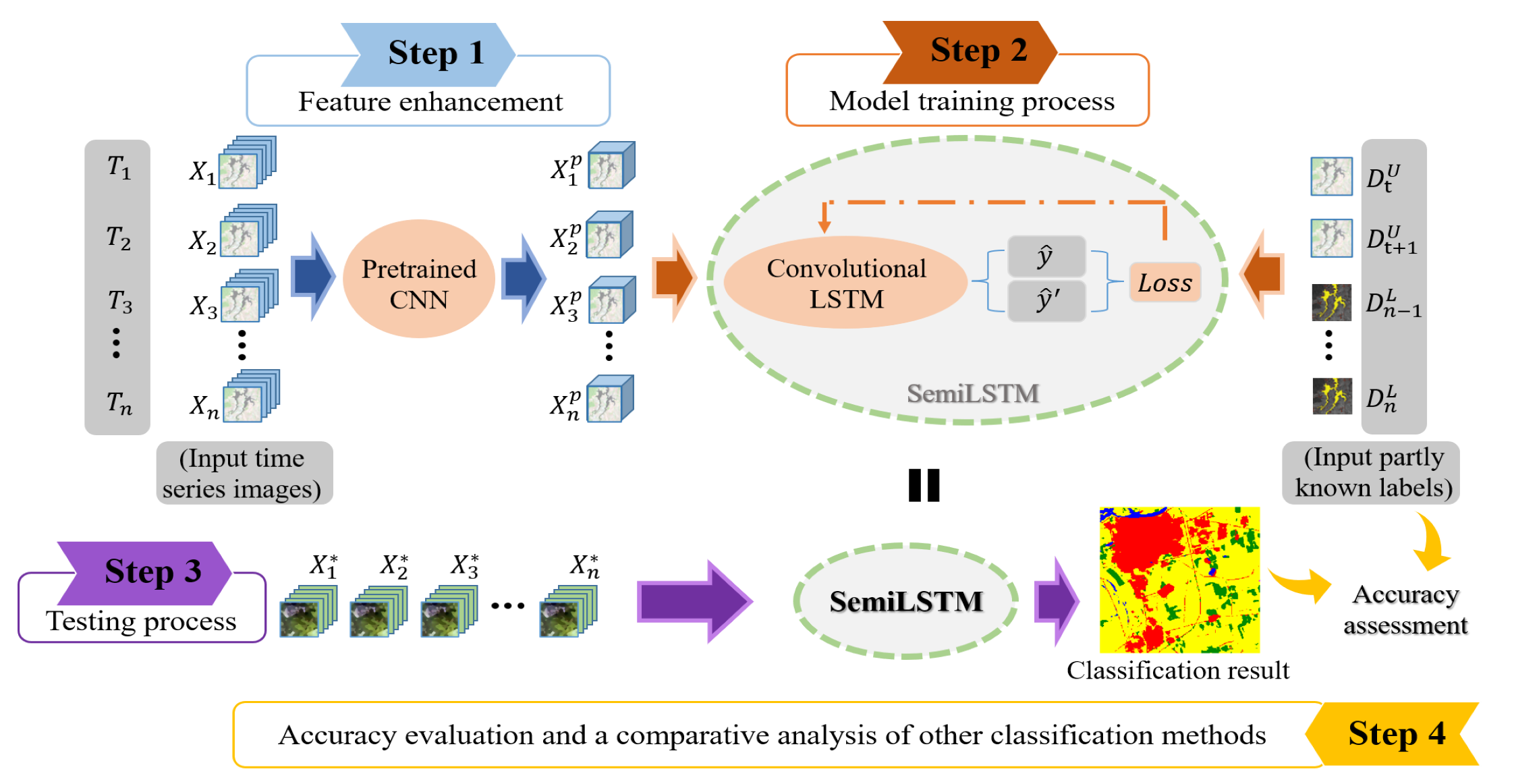
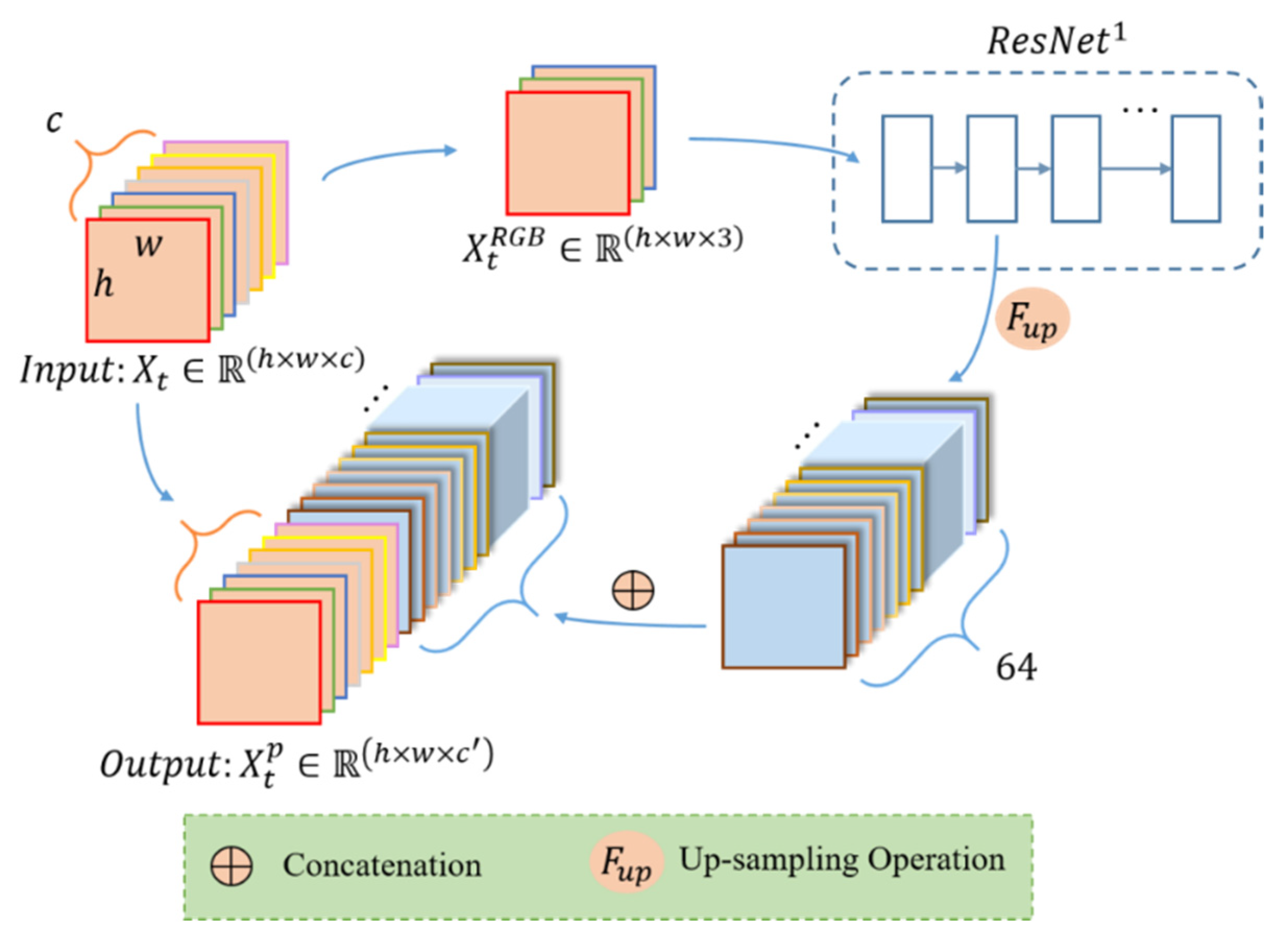
In the part 1, the initial input is a multispectral image , , from time series data set, and the output is an image with enhanced spatial feature representations , (), as shown in Figure 2. Since the ResNet was trained from natural images with red, green, and blue channels, the data we input to the ResNet pretrained model are the RGB image from original multispectral image. When input to the trained ResNet model, we choose the feature map after the first convolutional layer (expressed as ) to enhance the spatial features of details like textures and edges. Because for our low- and middle-resolution remote sensing images, the deeper convolution layer, the more spatial and texture features will be lost. With the processing of the deep convolutional network, the image’s resolution is getting smaller and smaller [35,36]. Thus, the original height h and width w are reduced, and the number of channels is increased to 64 after the size of convolution kernel. Then, the extracted feature map from is upsampled by bilinear interpolation to restore the same h and was the original image. At this time, the enhanced spatial information has been received. To further retain the multispectral information, the feature map after upsampling operation is concatenated with the original multispectral image. In the end, we get a new time series data after the pretrained model.
2.2. The Semi-Supervised Convolutional LSTM
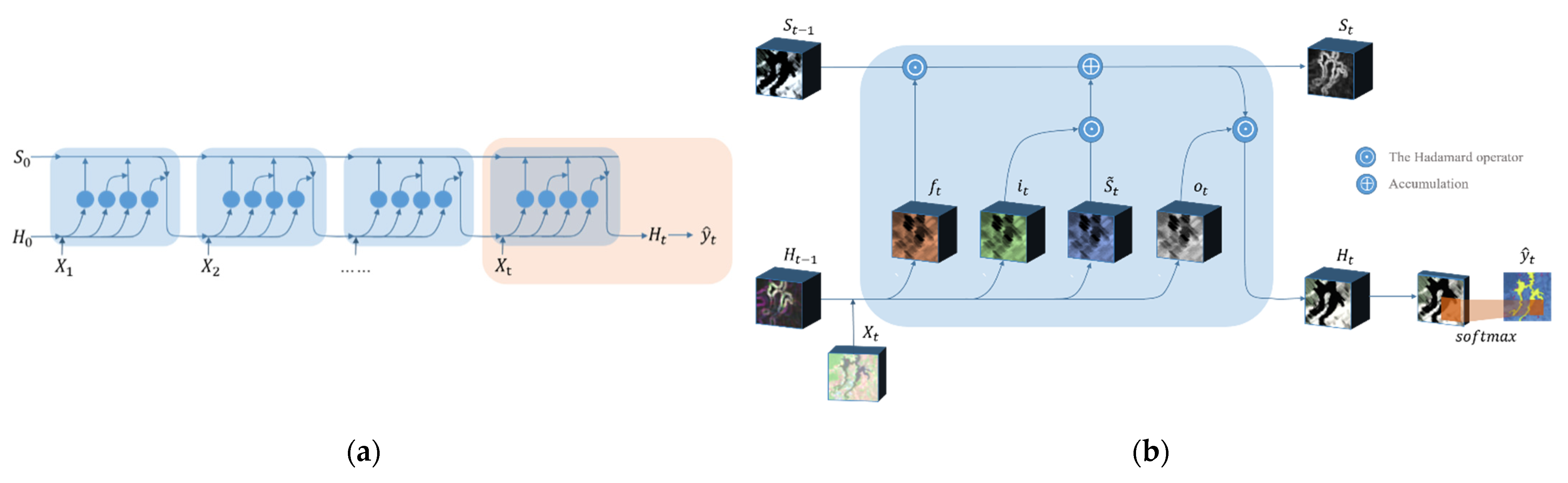
LSTM has been proven to have the ability to preserve long-term and short-term memory, it can effectively solve vanishing and exploding gradient problems of simple recurrent neural network for long sequence training data [19,37,38]. Due to the fully connected network structure, LSTM needs to convert three-dimensional images into vectors for pixel-level training when processing time series imagery. At this time, the spatial relationship between pixels and adjacent pixels is also lost. Owing to the capability of the convolution operations to process spatial information, some scholars have proposed variant LSTM networks with convolution structures [23,24]. Thus, when processing time series data, the spatial characteristics of images are preserved. This is conducive to processing remote sensing images with complex and diverse characteristics. For the training process of traditional deep learning networks, most of them rely on plentiful prior knowledge and sample selection. In the practical application of remote sensing data, it not only increases the workload of labeling samples, but also increases the difficulty of seeking suitable training samples in the limited remote sensing database. Therefore, we proposed a semi-supervised LSTM network with convolutional structures to deal with the land cover classification of long time series remote sensing images. Next, the training process of this network is described in detail.
After the pretrained model, a new set of time series data is constructed from the feature-enhanced images. In order to improve the computational efficiency and training effect of the temporal model, it is divided into numerous time series subdata sets with the same time series length (t), as shown in Figure 2, like In Figure 3a, we take the sequence subdata set as an example. The self-looping structure based on recurrent neural network can be regarded as a connection with multitudinous neural units. The weights among hidden layers are shared, which makes the network have memory capabilities. There are three gate mechanisms (input gate , forget gate , and output gate that jointly control the memory of long-term and short-term knowledge of neural units. As an input is fed, a current memory cell state can be obtained by the following equation, which gathers the current input and the previous hidden state .
where represents the hyperbolic tangent function. is the weight matrix from input to memory cell. denotes the hidden-memory coefficient matrix. is a bias coefficient and the symbol “” denotes the convolution operator with 3 × 3 pixels.
As each datum is input in sequence, the long-term memory will be accumulated and updated from both , which is controlled by the input gate , and the past memory cell state which controlled by the forget gate . The two gates and respectively control how much relevant information is added from and how much irrelevant prior information is omitted from . They can be expressed by the following formulas:
where represents the sigmoid function. , , , and denote the weight matrices from input data to input gate and forget gate, and from hidden state to input gate and forget gate, respectively. and are bias coefficients, and “”denotes a Hadamard product. Correspondingly, the memory cell state is updated by
Subsequently, is further controlled by the output gate and propagates to the final hidden output . is designed to determine how much memory content is output at the current moment t. The output gate and the short-term memory can be expressed as follows:
Owing to the convolutional operations between input-to-state and state-to-state transitions, as shown in Figure 3b. Compared with the traditional LSTM, it can better preserve spatial information and reduce the redundancy of spatial data in the process of temporal context information modeling. Due to the many-to-one network form, each sequence input has only one output, i.e., the sequence subdata set outputs the latest state . After that, enters a convolutional layer with a kernel size of 3 × 3 and a convolution stride of 1 pixel for decoding, which converts the high-dimensional features into the categories. Then, it is mapped to [0, 1] through the SoftMax function to obtain the predicted probability value . For our time series imagery classification task in Part 2, each image in time series subdata sets is sequentially passed to the convolutional LSTM encoder, and finally the prediction of is output.
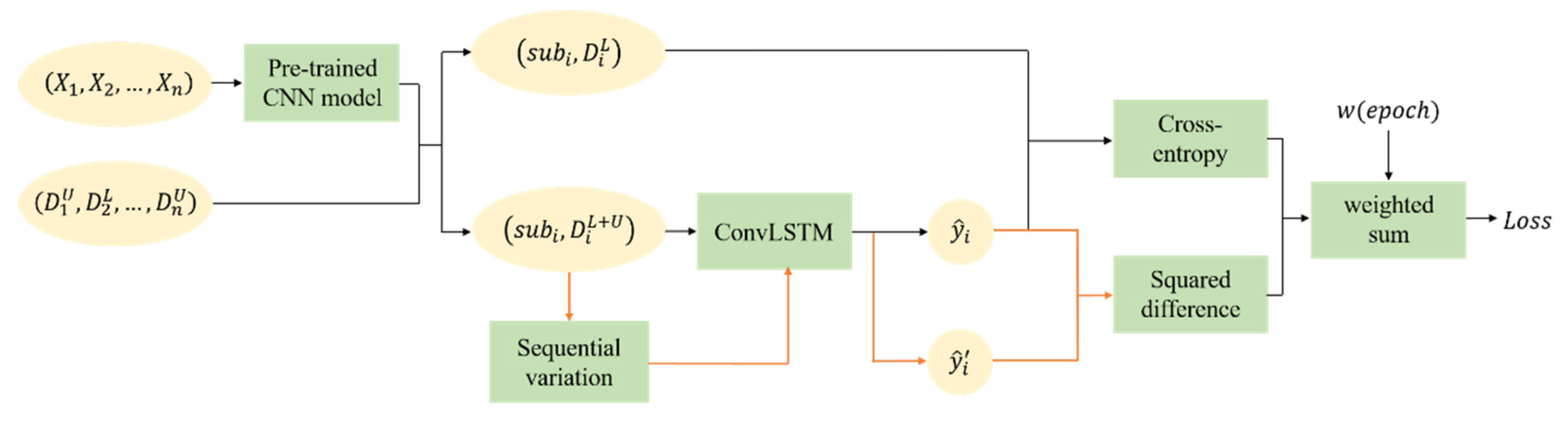
For traditional training process of networks, the loss function is defined as the standard cross-entropy which is calculated by the predicted label and respective reference label from ground truth data . This is essentially a supervised classification that needs large enough labels for training. Actually, the corresponding reference labels are mixtures with labeled and unlabeled data for the classification task of long time series remote sensing data, rather than known labels for every image. Thus, semi-supervised learning inspired by -model [39] is utilized. The structure of semi-supervised learning and the calculation of loss function is shown in Figure 4, and the pseudocode of training process in Algorithm 1. The function consists of supervised and unsupervised loss components. One is the standard cross-entropy between models’ predictions and reference labels , evaluated for known labels only. Because of the class imbalance, the tunable focusing parameter and the balance factor are used to balance the imbalanced proportion of positive and negative samples [40]. The other is evaluated for all inputs with labeled and unlabeled data. After the random sequential variation, the same time series input data produce two different predicted vectors from hidden layers, and . Then the mean square difference between these two values is made which can be seen as an error in classification. Besides, the latter is scaled by the loss weighting function related to the number of training times to merge the two loss items. The initial value of is set to , i.e., the loss value of the unsupervised part is not calculated. Through new inputs and continuous iterative calculations, the value of ramps up. It is very important that the unsupervised loss component must be promoted slowly enough, otherwise the network could easily fall into a degenerate solution and fail to achieve a meaningful classification effect. Finally, the optimizer is utilized to minimize the combined loss value to complete the optimization of the model parameters. It should be noted that one-hot encoding [41] is a smart way to demote ground truth values of different categories for multi-classes tasks.
| Algorithm 1. The training pseudocode of SemiLSTM. | |
| Require:, the time series subdata sets with the same time length (t) after pre-trained model ), for example, === ; | |
| Require: is the label corresponding to the last phase of , where unlabeled samples are represented as (C is the number of classes), and labeled samples are represented as ; | |
| Require:, the unsupervised weight ramp-up function; | |
| Require:, the convolutional LSTM with trainable parameters ; | |
| Require:, the time series input with random sequential variation function; | |
| Require:, the balance factor, is a constant vector whose length is the number of categories C; | |
| Require:, the tunable focusing parameter, is a constant. | |
| for epoch in [1, num_epochs] do: | |
| for i in [1, ] do: | |
| ▪Predictions for original sequential input | |
| ▪Again, with random sequential variation | |
| ▪Unsupervised loss component | |
| ▪Supervised loss component | |
| update using, e.g., | ▪Update network parameters |
|
end for end for | |
| return , | |
3. Study Areas and Data Sets
In our experiments, we used three sets of time series optical remote sensing data to verify the proposed method. The details are described as follows.
3.1. Jiamusi
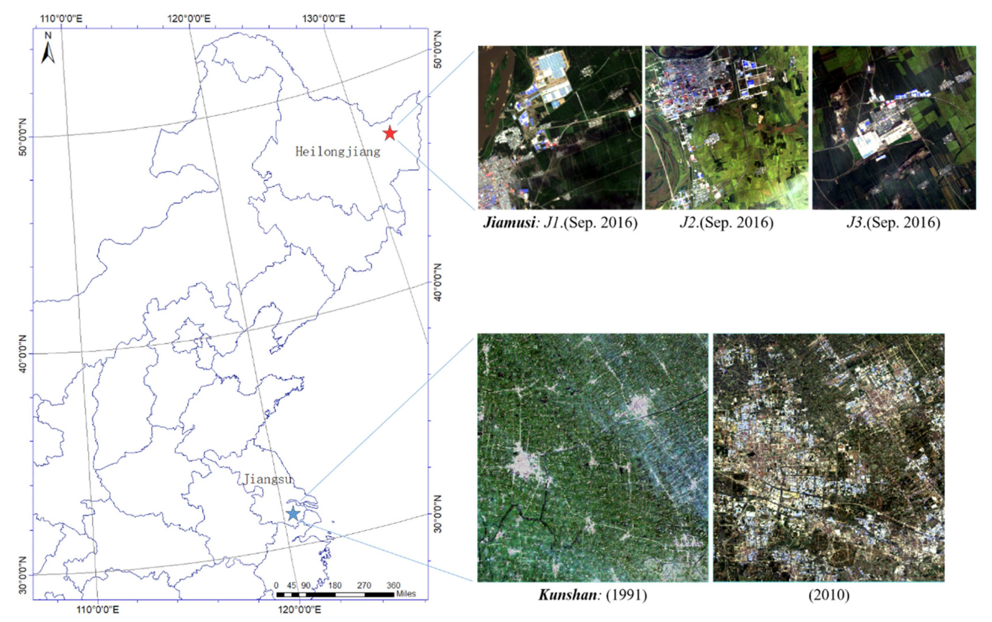
This data set was acquired by the Landsat 8/OLI sensor with a coordinate range of 45°42′′–48°31′N, 129°22′–129°42′E in Heilongjiang Province, China. Here, we only adopted seven bands with 30 m spatial resolution (B1–B7). There are three typical areas (J1/J2/J3) mainly based on urban expansion and natural phenology of various crops from 2015 to 2016. Each area covers 256 × 256 pixels of about 60 km2, as shown in Figure 5 (where marked by the red star). Due to a 16-day revisit cycle and free resources of satellite, there are a total of 26 available images with cloud-free or low cloud coverage, with an average of 1 to 2 images per month.
Besides, it covers six categories according to the actual situation, involving cultivated land, forest (including unused land), construction (incorporated buildings and roads), water, cloud, and shadow. Figure 6b illustrates the ground truth information of the last images (J1/J2/J3). The distribution of the categories is imbalanced due to human activities. The proportion of each category is 65.20%, 9.38%, 22.29%, and 3.13% respectively. Clouds and shadows are easy to appear in summer, usually from June to August, and their coverage varies. In the past two years, forests and water have basically remained unchanged, whereas cultivated lands and constructions have completely undergone different changes. With the increase in time, the building area has an obvious growth trend. In time series images with monthly intervals, cultivated land may first be converted to bare land, and then converted to construction land. Due to the natural growth of crops, cultivated land has obvious seasonal change rules, and has different spectral reflectance values in different seasons. It is conceivable that varying degrees and regular changes will increase the difficulty and accuracy of identifying land cover.
In the time series data, the image of each time corresponds to a label, but the known label is randomly distributed. Some known labels correspond to the real class values, whereas other unknown labels are 0. In training process, we further cropped images into many blocks with a size of 32 × 32 pixels as shown in Figure 6a. Among them, the blue boxes represent the training samples, and the orange boxes represent the testing samples. The distribution of the training and testing sets is random (i.e., J1, J2, and J3 have different sample distributions), but the sample ratio is still 1:3.
3.2. Kunshan
This data set is acquired by the Landsat 5 and 7 sensors from 31°15′–31°32′N, 120°54′–121°12′E, namely Kunshan city of China. Only six bands are used here: B1–B5 and B7 from two satellites with same 30 m spatial resolution and wavelength range. This area covers 1005 × 937 pixels about 848 km2 in Figure 5, marked by the blue star. It mainly shows urban expansion from 1991 to 2010 with a total of 20 images, where one image per year.
This time series data with annual intervals should be composed of annual cloudless images as much as possible. Compared with the monthly interval Jiamusi data set, it does not consider the coverage of clouds and shadows. It covers four types of labeled values, containing cultivated land, forest, construction, and water. Figure 6c shows the label information in 1991 and 2010, and the gray boxes represent only a small part of the large-scale data set. In the past 20 years, there had been a significant urban expansion phenomenon. The area of construction land had increased from 18.61% to 34.37%, while the area of cultivated land had decreased from 66.26% to 43.42%. In 2010, the coverage of forests and water were 7.40% and 14.81%, and both showed the same growth trend, with an increase of 3.93% and 3.15% respectively.
Similarly, in training process, the known labeled data are randomly distributed. In time series data with land changes, there may be only two phases with ground-truth labels. After cropping numerous image blocks (32 pixels × 32 pixels), we randomly selected the training and testing data with the same ratio (3:1).
3.3. Munich
This data set can be downloaded on GitHub [20]. It consists of cropped image blocks with a size of 48 × 48 pixels, derived from the 102 km × 42 km Sentinel 2 image in the north of Munich, Germany. In our experiments, we only used part of the available images in 2016 with a time length of 30 due to the limited computational space. There are four 10 m (B2, B3, B4, B8), six 20 m (B5, B6, B7, B8A, B11, B12), and three 60 m (B1, B9, B10) bands. At the time of input, the 20 m and 60 m bands were bilinear interpolated to 10 m ground sampling distance.
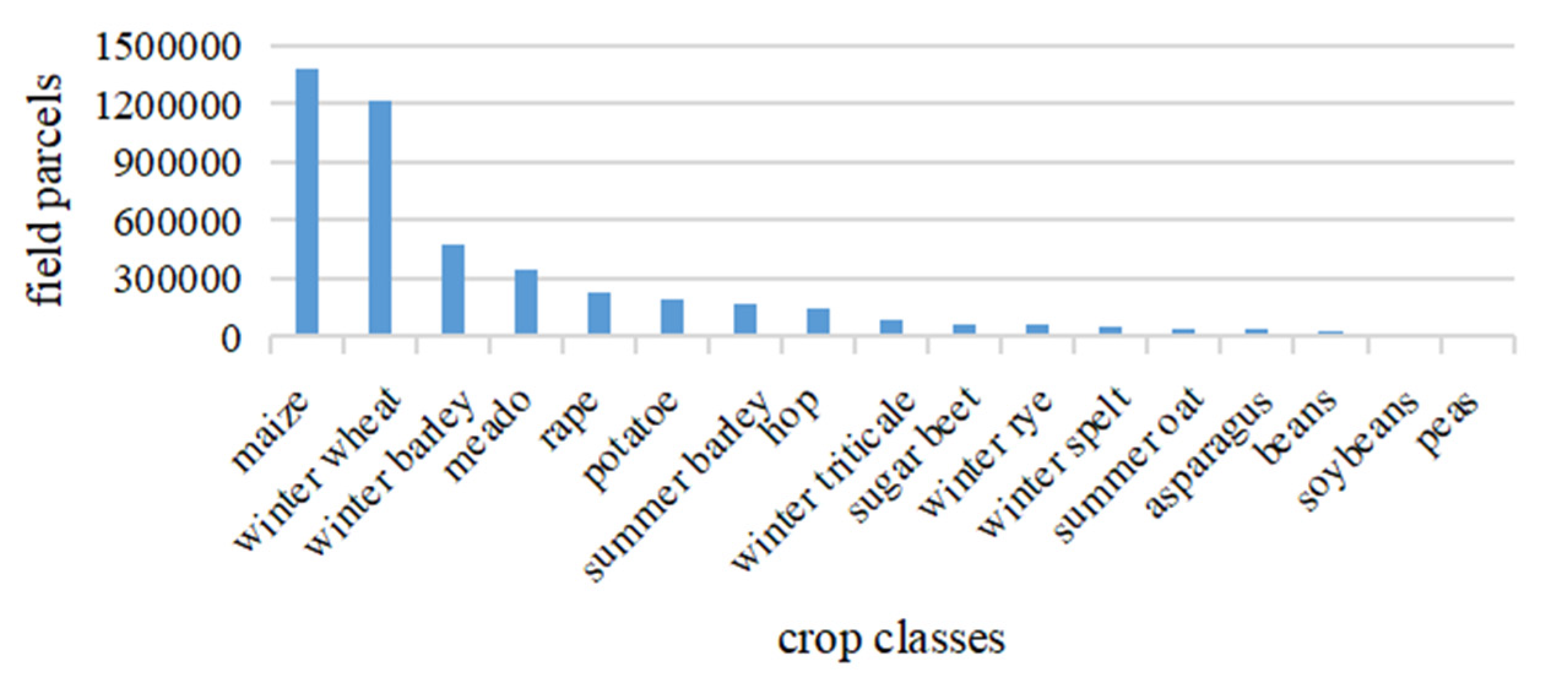
The ground truth information contains 17 crop categories, and only partial labeled samples are used. The non-uniform distribution of categories is shown in Figure 7. Similarly, we randomly selected the training and testing image blocks at a ratio of 3:1. Unlike Jiamusi and Kunshan time series data sets, its basic assumption is that the land cover has not changed. In other words, there is only one known label for Munich time series data set.
4. Experiments and Results
4.1. Experiments Setup
In order to verify the feasibility and effectiveness of our SemiLSTM method for time series images classification, LSTM-based methods (ConvLSTM and LSTM) and non-deep learning classifiers (SVM and RF) were selected as comparison methods. All models with various parameter values were repeatedly tested on the Window 10 platform with a single NVIDIA RTX 2080 Ti GPU (memory 11 GB) and a CORE i7-7800 × CPU. Deep learning network models based on RNN (SemiLSTM, ConvLSTM, and LSTM) were implemented in Python with the help of Tensorflow. The neural units of three networks were the same 256, the learning rate was 0.001, and the optimal lengths (t) of time series input in different data sets were different, where t = {20, 18, 30} in Jiamusi, Kunshan, and Munich respectively. More details and analyses are provided in Section 5.1. For ConvLSTM and our SemiLSTM models, owing to the convolutional kernel size of 3 × 3, we fed eight cropped 3D image blocks (h, w, c) as a batch into the networks. The difference in LSTM was that each image block was reshaped to a two-dimensional vector (h × w, c) as an input. Therefore, the batch was the number of pixels in an image block (h × w).
For non-deep learning classifiers (SVM and RF), we employed the Scikit-learn framework. Similar to the input of LSTM, image blocks needed to be transformed into a vector. However, these two methods cannot directly deal with temporal features. For this reason, we connected the time dimension with the spectral dimension. That is, the spectral channels of each image were superimposed together in chronological order, which was regarded as the channels of the entire image. It was necessary to assume that the surface information has not changed. To deal with imbalanced samples, class weight = “balanced”, so that each class had a weight based on the size of training samples [42]. We also adopted a random search strategy [43] to automatically pick the major optimal parameter values of model. For SVM, the RBF kernel was used, the candidate parameters C{0.1, 0.3, 1, 3, 10, 30, 100, 300} and gamma{0.1, 1, 2, 10, ‘auto’}. For RF classifier, the candidate parameters n_estimators{120, 300, 500}, max_depth{5, 15, 25, None}, min_samples_split{2, 5, 15, 25}, min_samples_leaf{1, 2, 5, 10}, and max_features{‘log2′, ‘sqrt’, None}.
In addition, although we randomly selected training and testing samples at the same ratio, for comparison experiments between different classifiers the random sampling of the same time series data remained consistent. In order to more fairly evaluate the effects of various classifiers, all models’ inputs were enhanced images after the same pretrained CNN model.
4.2. Accuracy Assessment of Classification
To evaluate the performance of various classifiers in various time series data sets, the following indicators were utilized: Overall accuracy (OA), Kappa coefficients (K), and the weighted F1 score (W-F1). All the evaluation indexes were employed in Scikit-learn package of Python. The optimal parameters of various models in detail were selected in previous section. The results are displayed in Table 1.
SVM and RF as the non-deep learning methods performed well with small training data set, which have been widely used in classification [44,45,46,47,48]. In our experiments of these various data sets, the results of the two models were similar and not good at the areas with varying and complex surface coverage. Moreover, they were time-consuming to repeat parameter selections by the random search strategy when entering a new data and process the data with high dimensions which combine the time and channel dimensions. SVM takes about two hours to complete an epoch in Jiamusi. If more parameters to be selected, like RF, it will take more time.
LSTM, as a variant RNN with three gates, is widely used because of its ability and advantage in processing temporal context information. Three LSTM-based networks had better performance on three different time series data, compared with non-deep learning classifiers which are based on the assumption of invariant land cover information. The three methods are far less time-consuming than the non-deep learning methods. Among them, LSTM can complete an epoch approximately every four minutes in Jiamusi, while ConvLSTM and SemiLSTM can complete an epoch approximately every one minute. In theory, ConvLSTM avoids the spatial features that may be lost in the data conversion process through convolution operations, so ConvLSTM had a slight advantage over LSTM (as shown in Table 1, the weighted F1 score of ConvLSTM was increased by 0.16, 0.07, and 0.05 in the Jiamusi, Kunshan, and Munich respectively). As for our proposed SemiLSTM method, its classified performance was better than LSTM and ConvLSTM in all data sets. For example, in the classification of Kunshan data set, the classification accuracy OA of SemiLSTM was improved by 12.11% compared with LSTM, and was increased by 5.58% compared with ConvLSTM. This is because the addition of semi-supervised learning made the model less dependent on known labeled samples, thereby reducing the interference of negative samples on land cover classification. Moreover, our method had a prominent classified performance in the case of a small number of known labels and the lack of images due to cloud occlusion. The related experimental analysis is described in Section 5.2 and Section 5.3 below. It solves the problems of poor representation of training samples and inevitable cloud occlusion on optical images to some extent.
5. Discussion
5.1. The Importance of Temporal Context Information
Temporal features play an important role in classification of remote sensing imagery. For instance, different types of crops have different seasonal phenological characteristics in crops classification, and the use of temporal context features can well distinguish various types of crops [18,44]. Temporal context features are beneficial to image classification tasks, especially in areas with land cover changes. But what length of time is the favorable condition for image classification?
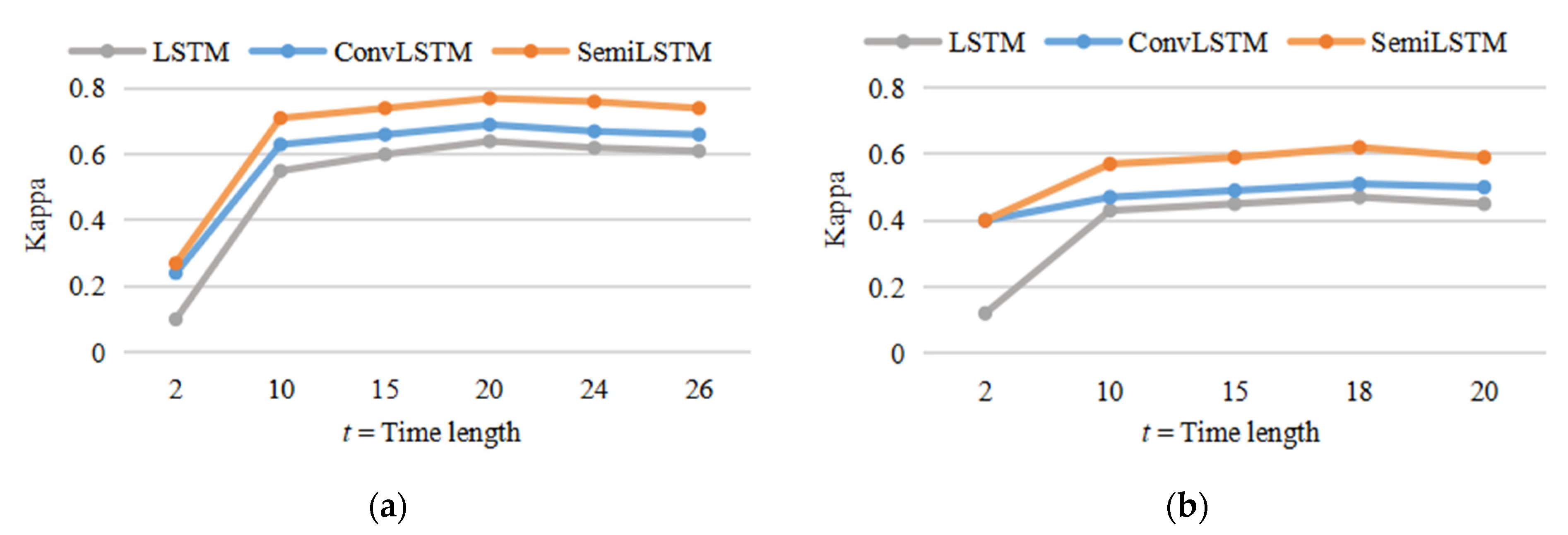
To find the optimal time length of time series image classification, we compared classification experiments with time series inputs of different lengths. We set a fixed time length (t) and extracted multiple subdata sets of time length t from the original sequence data in chronological order as the time series input of network. A loop was not executed until the last time node of the original time series data. Here, the Jiamusi and Kunshan were used for comparative experiments, because their time series data sets have equal interval time distribution and certain land cover changes. Therefore, the length of time series input t = {2, 10, 15, 20, 24, 26} in Jiamusi and t = {2, 10, 15, 18, 20} in Kunshan.
The OA metric of different time series lengths has the same change trend as the Kappa, but the change range is relatively small. Therefore, only the change of Kappa is shown in Figure 8. As the increase in length t, the classification effect was significantly improved. Since the total length of time series data was limited, the larger the t, the smaller the number of iterations. Therefore, as t increased, the accuracy of classification generally improved on a stable trend, or even decreased slightly. Just as human beings become obscure to longer-term memories, the larger length of time series, the memory of the deep neural network may be lost during the continuous updating process. It shows that it is necessary to appropriately increase the length of time series input and is conducive to land cover classification, rather than the larger time series length.
In addition, as shown in Figure 8, although the experimental results in the Jiamusi and Kunshan data sets show similar trends, the optimal parameters are different due to different time resolutions and research areas. Therefore, the parameter selection of the time series length needs to consider many factors such as time resolution, the size of the research area, and the complexity of the land surface. In this experiment, the optimal time series lengths in Jiamusi and Kunshan were 20 and 18, respectively. Moreover, the optimal parameters t were used in the subsequent comparison experiments.
5.2. Appropriate Number of Labeled Training Data
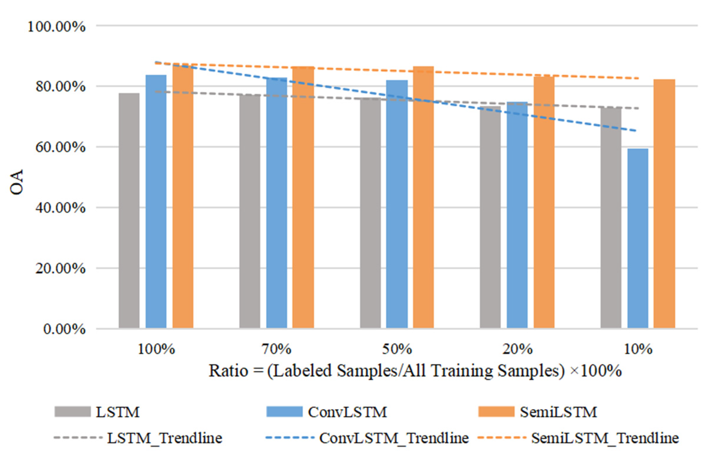
Supervised deep learning methods such as LSTM and ConvLSTM require a large number of known labels for training. But in practical application, it is hard to obtain enough labels, especially for a long time series data. The method proposed in this paper makes it possible to use a small proportion of labeled training samples and obtain excellent classification results, owing to the idea of semi-supervised learning. It will greatly reduce the requirements and workload of training labels, and make the classification and analysis of time series data easier to implement which can be widely used in various fields.
In order to explore the effect of the number of known labels on training process, five comparative experiments were set up, in which the labeled samples accounted for 100%, 70%, 50%, 20%, and 10% of the total training samples respectively. The number of known labels under different proportions were rounded down, that is the smallest integer was taken. Due to the limited length of Kunshan data and only one label in Munich, we conducted these comparative experiments in Jiamusi. Therefore, the experiments where the number of known labels account for 10%, 20%, 50%, 70%, and 100% were that only the last 2, 5, 13, 18, and 26 labeled samples were retained for training. The labels of other time nodes were filled with null values to represent unlabeled training samples, so that the total length of time series data was still 26. As described above in Section 5.1, the length of time series input t = 20. Due to the many-to-one networks, the known labels before were not used actually. When the ratios of known labels were 100%, 70%, and 50%, the classified results (OA) were similar.
Figure 9 illustrates the results on the different numbers of known training labels, where the dotted lines are a linear fit to OA values, indicating the trends of different models with the number of labeled samples. As the number of labeled samples decreased, the classified performance of SemiLSTM model became more prominent. Because of the semi-supervised training method, it reduced the dependence on a large number of known training samples. Compared with LSTM and ConvLSTM models, our model can still achieve a more accurate classification with a small number of known samples.
In short, reducing the model’s dependence on training samples is beneficial to image classification tasks. It not only reduces the difficulty of collecting time series labeled data (especially in complex environments and terrain conditions), but also reduces the cost and workload of labeling samples.
5.3. Cloud-Robust
More and more optical satellites monitor the dynamic spatiotemporal processes of the earth’s surface in a regular time with a few days intervals. However, satellite images are inevitably lost, as the surface is usually completely or partially covered by clouds. It limits the extensive research and application of majority remote sensing approaches, and brings great challenges for the methods that are designed with cloud-free imagery in mind.
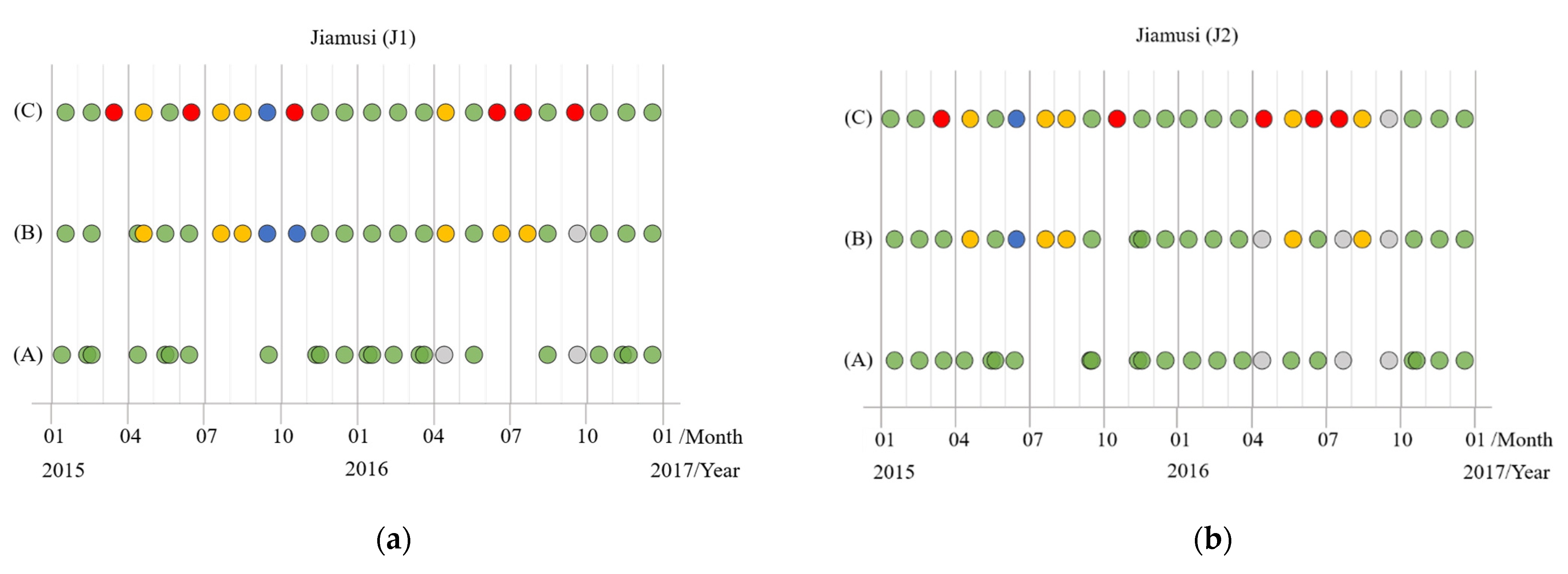
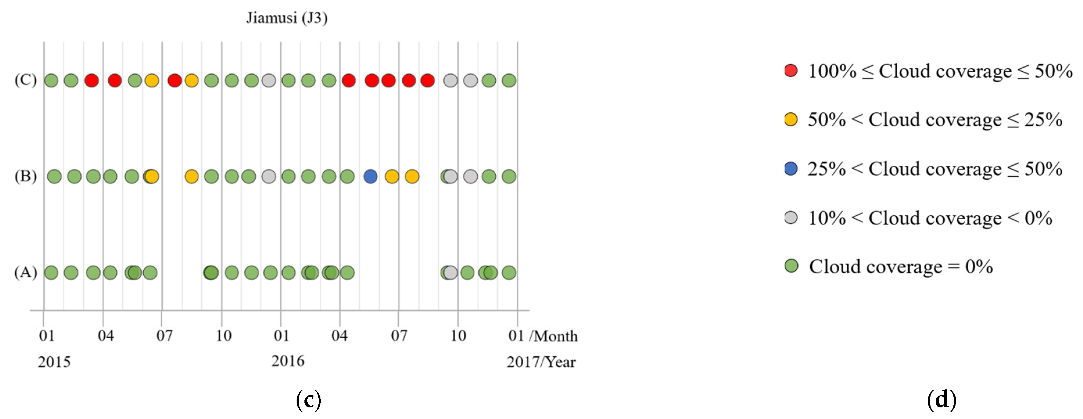
Therefore, we simulated time series images with different degrees of cloud coverage. Since the overlap of some original satellite images in Jiamusi, we had supplemented more abundant J1, J2, and J3 data from 2015 to 2016, including images with full or thick cloud coverage. Then it was further filtered and divided into time series subdata sets with the same total length (the length is 24 here). The time distribution of each subdata set in the three regions is displayed in Figure 10, and various color annotations indicate varying degrees of cloud coverage images. It should be noted that the cloud coverage is calculated by ROI (region of interest) from the clipped area. Moreover, only the labels of cloud-free images were reserved for the training process (the green circles in Figure 10), whereas other images with clouds had no known labels to participate in training.
Finally, there are three types of subdata set with different degrees of cloud coverage in each experimental region:
(A), The subdata set is basically full of cloud-free coverage images, and only a few are low-cloud coverage images. But such data set is difficult to guarantee the distribution of equal time intervals, and some data may be continuously missing for months (like the subdata set (A) in J3 which has no data for up to five months). We call this phenomenon “the lack of time series data”.
The subdata set (B) is composed of images with cloud coverage less than 50%, making the time series images distributed as uniformly as possible. However, there are still cases where no data in individual months, and remote sensing data of adjacent time phases are used instead.
In the subdata set (C), it contains images obscured by full or thick clouds (we called it “the lack of image data”), but its time series data is continuous and evenly distributed. In other words, there is an image every month.
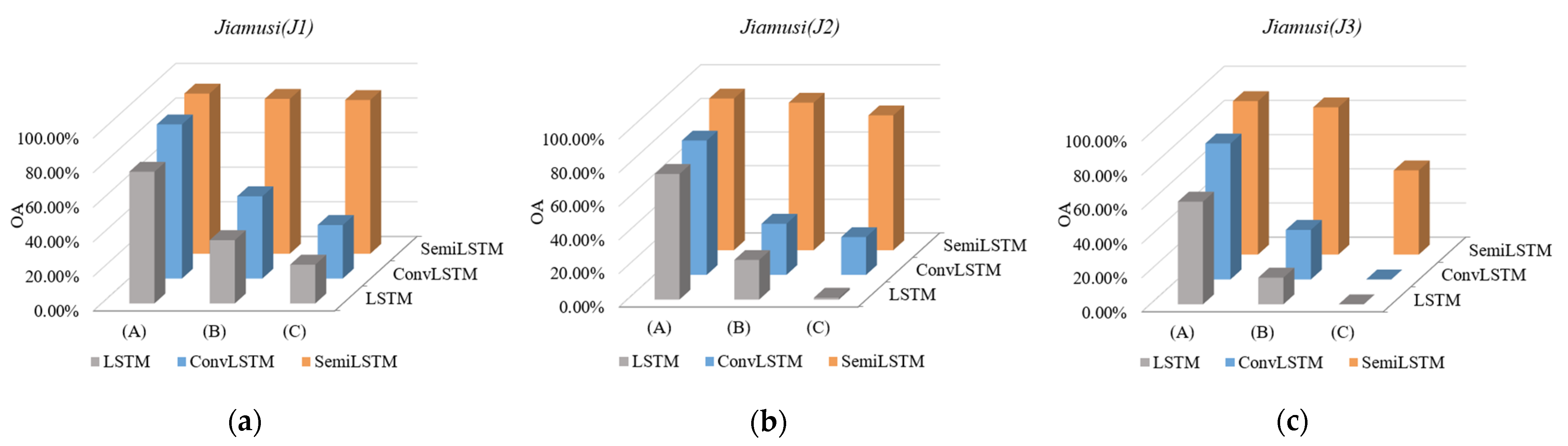
On this basis, we trained different deep neural networks to conduct comparative experiments on the above-mentioned time series subdata sets with different cloud coverage. The results (OA) of their predicted classification are shown in Figure 11. Among the three sets of experimental results, our SemiLSTM network had a robust classification regardless of the lack of time series data or image data. It shows that the semi-supervised learning method can not only reduce the dependence on samples, but also reduce the interference in clouds and shadows (negative samples) on the network training. It makes SemiLSTM model have a certain ability to resist the interference in clouds and learn features from other areas with cloudless coverage.
Besides, in the comparative experiments of subdata sets (A), (B), and (C) with different degrees of data missing, classification results of (C) were relatively poor even using the semi-supervised method. It can be seen that the lack of image data has a greater impact on classification than the lack of time series data. Thus, the data base without cloud coverage should be satisfied as much as possible in the application of time series images. In fact, optical satellite images are always difficult to avoid the interference of clouds and shadows (thick or thin coverage), such as subtropical areas that are easily blocked by clouds. At this time, our method still has good classification robustness.
6. Conclusions
In this study, we developed a novel deep neural network SemiLSTM to classify land cover by learning spectral-spatial-temporal features from time series remote sensing images. Compared with a variety of classification models (including non-deep learning and deep learning models), it has a more prominent classified performance. Among three LSTM-based deep learning networks, we verified that properly increasing the temporal length of time series input is conducive to land cover classification. Owing to the advantages of semi-supervised learning, our SemiLSTM model reduces the dependence on training samples, so that it still has a good classification performance in the case of a small number of known training labels. In addition, we supplemented and reorganized time series subdata sets with different cloud coverage to simulate the real situations of optical remote sensing images for comparison experiments. It shows that the lack of image data has a more serious impact on classification accuracy than the lack of time series data, but our SemiLSTM model is still robust for time series land cover classification with high cloud coverage. The study suggests that this classified method can reduce the requirements for data collection with abundant cloudless images or a lot of known labels, which is conductive to the application and promotion of the method. Moreover, it provides valuable help for optical remote sensing applications and research in areas that are seasonally or often obscured by clouds, such as subtropical areas.
Author Contributions
Conceptualization, C.T. and J.Q.; Data curation, J.S.; Formal analysis, J.S.; Funding acquisition, C.T.; Methodology, J.S., J.Q. and H.W.; Validation, J.S.; Writing—original draft, J.S.; Writing—review & editing, C.T., J.Q. and H.W. All authors have read and agreed to the published version of the manuscript.
Funding
The National Natural Science Foundation of China (No. 42171376, 41771458, 41871364); The Young Elite Scientists Sponsorship Program by Hunan province of China (No. 2018RS3012); Hunan Science and Technology Department Innovation Platform Open Fund Project (18K005); The Postgraduate Scientific Research Innovation Project of Hunan Province (CX20200325); The Fundamental Research Funds for the Central Universities of Central South University (2020zzts671).
Institutional Review Board Statement
Not applicable.
Informed Consent Statement
Not applicable.
Data Availability Statement
Publicly available datasets were analyzed in this study. The Munich time series data can be found here: https://github.com/TUM-LMF/MTLCC (accessed on 3 September 2021). The Jiamusi and Kunshan time series data can be found here: https://github.com/Sjing069/Time-series-remote-sensing-data (accessed on 3 September 2021).
Acknowledgments
The authors would like to thank all the colleagues for the fruitful discussions on this work. The authors also sincerely thank the anonymous reviewers for their very competent comments and helpful suggestions.
Conflicts of Interest
All authors declare no conflict of interest.
References
- Giri, C.; Pengra, B.; Long, J.; Loveland, T.R. Next generation of global land cover characterization, mapping, and monitoring. Int. J. Appl. Earth Obs. Geoinf. 2013, 25, 30–37. [Google Scholar] [CrossRef]
- Gross, J.E.; Goetz, S.J.; Cihlar, J. Application of remote sensing to parks and protected area monitoring: Introduction to the special issue. Remote Sens. Environ. 2009, 113, 1343–1345. [Google Scholar] [CrossRef]
- Hansen, M.C.; Egorov, A.; Potapov, P.V.; Stehman, S.V.; Bents, T. Monitoring conterminous united states (conus) land cover change with web-enabled landsat data (weld). Remote Sens. Environ. 2014, 140, 466–484. [Google Scholar] [CrossRef] [Green Version]
- Jin, S.; Yang, L.; Danielson, P.; Homer, C.; Xian, G. A comprehensive change detection method for updating the national land cover database to circa 2011. Remote Sens. Environ. 2013, 132, 159–175. [Google Scholar] [CrossRef] [Green Version]
- Lasanta, T.; Vicente-Serrano, S.M. Complex land cover change processes in semiarid mediterranean regions: An approach using landsat images in northeast spain. Remote Sens. Environ. 2012, 124, 1–14. [Google Scholar] [CrossRef]
- Xian, G.; Homer, C.; Fry, J. Updating the 2001 national land cover database land cover classification to 2006 by using landsat imagery change detection methods. Remote Sens. Environ. 2009, 113, 1133–1147. [Google Scholar] [CrossRef] [Green Version]
- Boles, S.H.; Xiao, X.; Liu, J.; Zhang, Q.; Munkhtuya, S.; Chen, S.; Ojima, D. Land cover characterization of temperate east asia using multi-temporal vegetation sensor data. Remote Sens. Environ. 2004, 90, 477–489. [Google Scholar] [CrossRef]
- Chen, Y.; Peng, G. Clustering based on eigenspace transformation—CBEST for efficient classification. ISPRS J. Photogramm. Remote Sens. 2013, 83, 64–80. [Google Scholar] [CrossRef]
- Pal, M.; Mather, P.M. An assessment of the effectiveness of decision tree methods for land cover classification. Remote Sens. Environ. 2003, 86, 554–565. [Google Scholar] [CrossRef]
- Belgiu, M.; Dragut, L. Random forest in remote sensing: A review of applications and future directions. ISPRS J. Photogramm. Remote Sens. 2016, 114, 24–31. [Google Scholar] [CrossRef]
- Mountrakis, G.; Im, J.; Ogole, C. Support vector machines in remote sensing: A review. ISPRS J. Photogramm. Remote Sens. 2011, 66, 247–259. [Google Scholar] [CrossRef]
- Bagan, H.; Wang, Q.; Watanabe, M.; Yang, Y.; Jianwen, M.A. Land cover classification from modis evi times-series data using som neural network. Int. J. Remote Sens. 2005, 26, 4999–5012. [Google Scholar] [CrossRef]
- Maulik, U.; Chakraborty, D. Learning with transductive svm for semisupervised pixel classification of remote sensing imagery. ISPRS J. Photogramm. Remote Sens. 2013, 77, 66–78. [Google Scholar] [CrossRef]
- Tao, C.; Qi, J.; Lu, W.; Wang, H.; Li, H. Remote sensing image scene classification with self-supervised paradigm under limited labeled samples. IEEE Geosci. Remote Sens. Lett. 2020. [Google Scholar] [CrossRef]
- Xu, P.; Song, Z.; Yin, Q.; Song, Y.Z.; Wang, L. Deep self-supervised representation learning for free-hand sketch. IEEE Trans. Circuits Syst. Video Technol. 2020, 31, 1503–1513. [Google Scholar] [CrossRef]
- Jamshidpour, N.; Homayouni, S.; Safari, A. Graph-based semi-supervised hyperspectral image classification using spatial information. In Proceedings of the 2016 8th Workshop on Hyperspectral Image and Signal Processing: Evolution in Remote Sensing (WHISPERS), Los Angeles, CA, USA, 21–24 August 2016. [Google Scholar]
- Khatami, R.; Mountrakis, G.; Stehman, S.V. A meta-analysis of remote sensing research on supervised pixel-based land-cover image classification processes: General guidelines for practitioners and future research. Remote Sens. Environ. 2016, 177, 89–100. [Google Scholar] [CrossRef] [Green Version]
- Jia, K.; Liang, S.; Wei, X.; Yao, Y.; Su, Y.; Bo, J.; Wang, X. Land cover classification of landsat data with phenological features extracted from time series modis ndvi data. Remote Sens. 2014, 6, 11518–11532. [Google Scholar] [CrossRef] [Green Version]
- Greff, K.; Srivastava, R.K.; Koutník, J.; Steunebrink, B.R.; Schmidhuber, J. Lstm: A search space odyssey. IEEE Trans. Neural Netw. Learn. Syst. 2016, 28, 2222–2232. [Google Scholar] [CrossRef] [Green Version]
- Rubwurm, M.; Korner, M. Temporal vegetation modelling using long short-term memory networks for crop identification from medium-resolution multi-spectral satellite images. In Proceedings of the IEEE Conference on Computer Vision & Pattern Recognition, Honolulu, HI, USA, 21–26 July 2017; pp. 1496–1504. [Google Scholar]
- Scott, G.J.; England, M.R.; Starms, W.A.; Marcum, R.A.; Davis, C.H. Training deep convolutional neural networks for land–cover classification of high-resolution imagery. IEEE Geoence Remote Sens. Lett. 2017, 14, 549–553. [Google Scholar] [CrossRef]
- Li, H.; Qiu, K.; Chen, L.; Mei, X.; Hong, L.; Tao, C. SCAttNet: Semantic segmentation network with spatial and channel attention mechanism for high-resolution remote sensing images. IEEE Geosci. Remote Sens. Lett. 2020, 18, 905–909. [Google Scholar] [CrossRef]
- Xingjian, S.; Chen, Z.; Wang, H.; Yeung, D.-Y.; Wong, W.-K.; Woo, W.-C. Convolutional lstm network: A machine learning approach for precipitation nowcasting. In Proceedings of the Advances in Neural Information Processing Systems, Montreal, QC, Canada, 7–12 December 2015; pp. 802–810. [Google Scholar]
- Mou, L.; Bruzzone, L.; Zhu, X.X. Learning spectral-spatial-temporal features via a recurrent convolutional neural network for change detection in multispectral imagery. IEEE Trans. Geosci. Remote Sens. 2019, 57, 924–935. [Google Scholar] [CrossRef] [Green Version]
- Gomez, C.; White, J.C.; Wulder, M.A. Optical remotely sensed time series data for land cover classification: A review. ISPRS J. Photogramm. Remote Sens. 2016, 116, 55–72. [Google Scholar] [CrossRef] [Green Version]
- Li, Y.; Chen, W.; Zhang, Y.; Tao, C.; Tan, Y. Accurate cloud detection in high-resolution remote sensing imagery by weakly supervised deep learning. Remote Sens. Environ. 2020, 250, 112045. [Google Scholar] [CrossRef]
- Brooks, E.B.; Thomas, V.A.; Wynne, R.H.; Coulston, J.W. Fitting the multitemporal curve: A fourier series approach to the missing data problem in remote sensing analysis. IEEE Trans. Geosci. Remote Sens. 2012, 50, 3340–3353. [Google Scholar] [CrossRef] [Green Version]
- Yuan, Y.; Meng, Y.; Lin, L.; Sahli, H.; Yue, A.; Chen, J.; Zhao, Z.; Kong, Y.; He, D. Continuous change detection and classification using hidden markov model: A case study for monitoring urban encroachment onto farmland in beijing. Remote Sens. 2015, 7, 15318–15339. [Google Scholar] [CrossRef] [Green Version]
- Jing, S.; Chao, T. Time series land cover classification based on semi-supervised convolutional long short-term memory neural networks. ISPRS-Int. Arch. Photogramm. Remote Sens. Spat. Inf. Sci. 2020, 43, 1521–1528. [Google Scholar] [CrossRef]
- Chen, Y.; Jiang, H.; Li, C.; Jia, X.; Ghamisi, P. Deep feature extraction and classification of hyperspectral images based on convolutional neural networks. IEEE Trans. Geosci. Remote Sens. 2016, 54, 6232–6251. [Google Scholar] [CrossRef] [Green Version]
- Marmanis, D.; Datcu, M.; Esch, T.; Stilla, U. Deep learning earth observation classification using imagenet pretrained networks. IEEE Geosci. Remote Sens. Lett. 2016, 13, 105–109. [Google Scholar] [CrossRef] [Green Version]
- Zhou, W.; Newsam, S.; Li, C.; Shao, Z. Learning low dimensional convolutional neural networks for high-resolution remote sensing image retrieval. Remote Sens. 2016, 9, 489. [Google Scholar] [CrossRef] [Green Version]
- He, K.; Zhang, X.; Ren, S.; Sun, J. Deep residual learning for image recognition. In Proceedings of the IEEE Conference on Computer Vision & Pattern Recognition, Las Vegas, NV, USA, 27–30 June 2016; pp. 770–778. [Google Scholar]
- Deng, J.; Dong, W.; Socher, R.; Li, L.-J.; Li, K.; Fei-Fei, L. Imagenet: A large-scale hierarchical image database. In Proceedings of the IEEE Conference on Computer Vision & Pattern Recognition, Miami, FL, USA, 20–25 June 2009; pp. 248–255. [Google Scholar]
- Erhan, D.; Bengio, Y.; Courville, A.; Vincent, P. Visualizing higher-layer features of a deep network. Univ. Montr. 2009, 1341, 1. [Google Scholar]
- Zeiler, M.D.; Fergus, R. Visualizing and Understanding Convolutional Networks. Available online: https://arxiv.org/abs/1311.2901 (accessed on 28 November 2013).
- Gers, F.A.; Schmidhuber, J.; Cummins, F.A. Learning to forget: Continual prediction with LSTM. Neural Comput. 2000, 12, 2451–2471. [Google Scholar] [CrossRef]
- Hochreiter, S.; Schmidhuber, J. Long short-term memory. Neural Comput. 1997, 9, 1735–1780. [Google Scholar] [CrossRef] [PubMed]
- Laine, S.M.; Aila, T.O. Temporal ensembling for semi-supervised learning. In Proceedings of the 5th International Conference on Learning Representations, Toulon, France, 24–26 April 2017. [Google Scholar]
- Lin, T.Y.; Goyal, P.; Girshick, R.; He, K.; Dollár, P. Focal loss for dense object detection. IEEE Trans. Pattern Anal. Mach. Intell. 2017, PP, 2999–3007. [Google Scholar]
- Chren, W.A. One-hot residue coding for high-speed non-uniform pseudo-random test pattern generation. In Proceedings of the International Symposium on Circuits and Systems, Scottsdale, AZ, USA, 26–19 May 2002. [Google Scholar]
- Zhong, L.; Hu, L.; Zhou, H. Deep learning based multi-temporal crop classification. Remote Sens. Environ. 2019, 221, 430–443. [Google Scholar] [CrossRef]
- Bergstra, J.; Bengio, Y. Random search for hyper-parameter optimization. J. Mach. Learn. Res. 2012, 13, 281–305. [Google Scholar]
- Carrao, H.; Goncalves, P.; Caetano, M. Contribution of multispectral and multitemporal information from modis images to land cover classification. Remote Sens. Environ. 2008, 112, 986–997. [Google Scholar] [CrossRef]
- Lawrence, R.L.; Wood, S.D.; Sheley, R.L. Mapping invasive plants using hyperspectral imagery and breiman cutler classifications (randomforest). Remote Sens. Environ. 2006, 100, 356–362. [Google Scholar] [CrossRef]
- Shi, D.; Yang, X. An assessment of algorithmic parameters affecting image classification accuracy by random forests. Photogramm. Eng. Remote Sens. 2016, 82, 407–417. [Google Scholar] [CrossRef]
- Zhang, J.; Feng, L.; Yao, F. Improved maize cultivated area estimation over a large scale combining modis–evi time series data and crop phenological information. ISPRS J. Photogramm. Remote Sens. 2014, 94, 102–113. [Google Scholar] [CrossRef]
- Na, X.; Zhang, S.; Li, X.; Yu, H.; Liu, C. Improved land cover mapping using random forests combined with landsat thematic mapper imagery and ancillary geographic data. Photogramm. Eng. Remote Sens. 2010, 76, 833–840. [Google Scholar] [CrossRef]
Figure 1.
The framework overview of the proposed SemiLSTM model for land cover classification in time series images.
Figure 1.
The framework overview of the proposed SemiLSTM model for land cover classification in time series images.

Figure 2.
The process of the pretrained model for each image.

Figure 3.
Schematic illustration of convolutional LSTM network architectures. (a) The process of convolutional LSTM for a time series input ; (b) a neural cell of input at time t, where the pink box in (a).
Figure 3.
Schematic illustration of convolutional LSTM network architectures. (a) The process of convolutional LSTM for a time series input ; (b) a neural cell of input at time t, where the pink box in (a).

Figure 4.
The process of semi-supervised learning and loss calculation of SemiLSTM.

Figure 5.
Study area locations of Jiamusi and Kunshan. We used three small areas (J1, J2, and J3) with the size of 256 × 256 pixels in Jiamusi from 2015 to 2016. The Kunshan data spans from 1991 to 2010, and the image size is 1005 × 937 pixels.
Figure 5.
Study area locations of Jiamusi and Kunshan. We used three small areas (J1, J2, and J3) with the size of 256 × 256 pixels in Jiamusi from 2015 to 2016. The Kunshan data spans from 1991 to 2010, and the image size is 1005 × 937 pixels.

Figure 6.
The ground truth information (GT) and data division. (a) The training samples (blue boxes) and testing samples (orange boxes) are randomly selected at a ratio of 3:1 from several equal-sized images blocks; (b) the labels of Jiamusi (J1, J2, and J3) in September 2016 (corresponding to the cloud-free images in Figure 5); (c) the labels of Kunshan in 1990 and 2010, where the gray boxes represent only a small part of the large-scale data set.

Figure 7.
Information of labeled samples and the non-uniform distribution of classes in Munich data set.
Figure 7.
Information of labeled samples and the non-uniform distribution of classes in Munich data set.

Figure 8.
The results (Kappa) of comparative experiments with various length of time series input in Jiamusi and Kunshan data set. (a) Jiamusi time series data set; (b) Kunshan time series data set.
Figure 8.
The results (Kappa) of comparative experiments with various length of time series input in Jiamusi and Kunshan data set. (a) Jiamusi time series data set; (b) Kunshan time series data set.

Figure 9.
The results of comparative experiments where the ratios of known labels are 100%, 70%, 50%, 20%, and 10% respectively. The dotted lines are a linear fit to OA values.
Figure 9.
The results of comparative experiments where the ratios of known labels are 100%, 70%, 50%, 20%, and 10% respectively. The dotted lines are a linear fit to OA values.

Figure 10.
The time series subdata sets with different cloud coverage in the three regions from Jiamusi, in which various colored circles represent images with varying cloud coverage. (a) J1; (b) J2; (c) J3; (d) the legend.
Figure 10.
The time series subdata sets with different cloud coverage in the three regions from Jiamusi, in which various colored circles represent images with varying cloud coverage. (a) J1; (b) J2; (c) J3; (d) the legend.


Figure 11.
The OA results of time series subdata sets with different cloud coverage (where (A), (B) and (C) represent subdata sets containing low-cloud, less than 50%-cloud and thick cloud coverage respectively). (a) J1; (b) J2; (c) J3.
Figure 11.
The OA results of time series subdata sets with different cloud coverage (where (A), (B) and (C) represent subdata sets containing low-cloud, less than 50%-cloud and thick cloud coverage respectively). (a) J1; (b) J2; (c) J3.


Table 1.
Overall accuracy (OA), Kappa coefficients (K), and weighted score (WF1) tested on various data sets.
Table 1.
Overall accuracy (OA), Kappa coefficients (K), and weighted score (WF1) tested on various data sets.
| RF | SVM | LSTM | ConvLSTM | SemiLSTM | ||
|---|---|---|---|---|---|---|
| Jiamusi | OA | 54.04% | 53.87% | 77.67% | 83.50% | 86.61% |
| K | 0.17 | 0.21 | 0.64 | 0.69 | 0.77 | |
| WF1 | 0.44 | 0.48 | 0.62 | 0.78 | 0.83 | |
| Kunshan | OA | 40.56% | 45.32% | 65.58% | 72.11% | 77.69% |
| K | 0.15 | 0.19 | 0.46 | 0.51 | 0.62 | |
| WF1 | 0.30 | 0.35 | 0.57 | 0.64 | 0.75 | |
| Munich | OA | 38.35% | 47.68% | 78.27% | 80.58% | 87.24% |
| K | 0.21 | 0.33 | 0.53 | 0.59 | 0.63 | |
| WF1 | 0.19 | 0.46 | 0.77 | 0.82 | 0.88 |
Publisher’s Note: MDPI stays neutral with regard to jurisdictional claims in published maps and institutional affiliations. |
© 2021 by the authors. Licensee MDPI, Basel, Switzerland. This article is an open access article distributed under the terms and conditions of the Creative Commons Attribution (CC BY) license (https://creativecommons.org/licenses/by/4.0/).
Share and Cite
MDPI and ACS Style
Shen, J.; Tao, C.; Qi, J.; Wang, H. Semi-Supervised Convolutional Long Short-Term Memory Neural Networks for Time Series Land Cover Classification. Remote Sens. 2021, 13, 3504. https://0-doi-org.brum.beds.ac.uk/10.3390/rs13173504
AMA Style
Shen J, Tao C, Qi J, Wang H. Semi-Supervised Convolutional Long Short-Term Memory Neural Networks for Time Series Land Cover Classification. Remote Sensing. 2021; 13(17):3504. https://0-doi-org.brum.beds.ac.uk/10.3390/rs13173504
Chicago/Turabian StyleShen, Jing, Chao Tao, Ji Qi, and Hao Wang. 2021. "Semi-Supervised Convolutional Long Short-Term Memory Neural Networks for Time Series Land Cover Classification" Remote Sensing 13, no. 17: 3504. https://0-doi-org.brum.beds.ac.uk/10.3390/rs13173504
Note that from the first issue of 2016, this journal uses article numbers instead of page numbers. See further details here.