Article

Evaluation of a Statistical Approach for Extracting Shallow Water Bathymetry Signals from ICESat-2 ATL03 Photon Data

by
Heidi Ranndal
1,*,
Philip Sigaard Christiansen
2,
Pernille Kliving
1,
Ole Baltazar Andersen
1 and
Karina Nielsen
1
1
DTU Space, Technical University of Denmark, Elektrovej 328, 2800 Kongens Lyngby, Denmark
2
Danish Geodata Agency, Lindholm Brygge 31, 9400 Nørresundby, Denmark
*
Author to whom correspondence should be addressed.
Remote Sens. 2021, 13(17), 3548; https://0-doi-org.brum.beds.ac.uk/10.3390/rs13173548
Submission received: 17 July 2021 / Revised: 23 August 2021 / Accepted: 28 August 2021 / Published: 6 September 2021

Abstract

:
In this study we present and validate a simple empirical method to obtain bathymetry profiles using the geolocated photon data from the Ice, Cloud, and Land Elevation Satellite-2 (ICESat-2) mission, which was launched by NASA in September 2018. The satellite carries the Advanced Topographic Laser Altimeter System (ATLAS), which is a lidar that can detect single photons and calculate their bounce point positions. ATLAS uses a green laser, causing some of the photons to penetrate the air–water interface. Under the right conditions and in shallow waters (<40 m), these photons are reflected back to ATLAS after interaction with the ocean bottom. Using ICESat-2 data from four different overflights above the Heron Reef, Australia, a comparison with SDB data showed a median absolute deviation of approximately 18 cm and Root Mean Square Errors (RMSEs) down to 28 cm. Crossovers between two different overflights above the Heron Reef showed a median absolute difference of 13 cm. For an area north-west of Sisimiut, Greenland, the comparison was done with multibeam echo sounding data, with RMSEs down to between 35 cm, and correspondingly showed median absolute deviations between 33 and 49 cm. The proposed method works well under good conditions with clear waters such as in the Great Barrier Reef; however, for more difficult areas a more advanced machine learning technique should be investigated in order to find an automated method that can distinguish between bathymetry and other signals and noise.

Graphical Abstract

1. Introduction

Mapping of bathymetry has been important for the safety of marine endeavours since long before modern times. The earliest development of bathymetric charts dates back to 1900 BC in Ancient Egypt [1]. In modern times, nautical charts are important not only for marine safety, but also for fish and marine industries and coastal management. In particular, near shore bathymetry is important for engineering, coastal safety, and environmental monitoring. In some places, shallow water bathymetry also changes with time due to erosion and sediment transport. For these reasons, it is essential that the bathymetry for coastal and shallow waters is mapped.
Mapping near coastal bathymetry requires a great effort. Traditionally, single-beam or multibeam echo sounders mounted on a ship are used. The time it takes for a beam of sound to travel from the ship to the seafloor and back reveals the depth at the time of measurement. Near-coastal ship measurements from single- or multibeam sonars are difficult to obtain, since they are hard to deploy close to the shore. They are also costly and require a lot of planning. Today, these kinds of high-resolution soundings of the seafloor can in some cases be carried out by remotely operated vehicles (ROVs) or autonomous underwater vehicles (AUVs) [2]. Another option is airborne lidar bathymetry, which also has the same limitations of being local or regional, as well as being expensive and time consuming. Global, shallow water bathymetry data can currently be obtained using multi-spectral satellite imagery from satellites such as WorldView, Landsat and Sentinel-2. This is usually referred to as Satellite-Derived Bathymetry (SDB). Various bands from satellite images are used together with empirical and/or physical models to derive depths. However, the training of these empirical models and calibration of the physical models requires another source of bathymetry or special atmospheric corrections. Using satellite imagery has a higher uncertainty, but has the benefit that it can be done quite easily for many remote areas simply by downloading often freely available imagery online.
Another approach which utilizes satellite imagery is two-media photogrammetry, which is a method that has been around for a long time [3,4]. In recent years, WordView-2 stereo imagery has been used to derive bathymetry estimates for depths ranging between 5 and 20 m with Root Mean Square Errors (RMSE) around 1–2 m [5,6]. In addition to satellite imagery, air-borne or even images from drones can be used to derive shallow water bathymetry. To perform two-media photogrammetry, no atmospheric corrections or in-situ data are needed, which in that sense makes it superior to SDB methods.
Both ICESat and ICESat-2 data have previously been used for bathymetry studies. In [7] they focused on Lake Poopó in Bolivia and used ICESat data to derive isolines from the lake boundaries during low water stages. During high water stages where these areas are inundated, the isolines were used to estimate changes in the water storage. In [8] ICESat-2 ATL03 bathymetry was derived for four different sites, where it was shown that bathymetry could be found for depths down to ≈40 m or a maximum penetration depth of around 0.96 Secchi. The study also performed the first validation of the bathymetric signals from ICESat-2 using in situ data in the area of St. Thomas, U.S. Virgin Islands. After applying a refraction correction they compared the ICESat-2 bathymetry to lidar data from the U.S. Geological Survey (USGS) and the National Oceanic and Atmospheric Administration (NOAA). They found a RMSE of around 0.43–0.60 m. In [9] they used a machine learning method to derive ICESat-2 bathymetry from the ATL03 data set. More specifically, they took advantage of a density-based spatial clustering algorithm called “dbscan” to derive the bathymetry. These bathymetries were then used as input for an empirical SDB model. The resulting SDB depths were validated using airborne lidar bathymetry data near Ganquan Island in the Yongle Atolls, and the resulting RMSE was 1.44 m. The ICESat-2 bathymetry data themselves were not validated. Other studies have also used ICESat-2 bathymetry together with satellite imagery, mostly from Sentinel-2, to derive Satellite Derived Bathymetry (SDB) in areas such as Florida, Crete and Bermuda [10], St. Croix in the U.S. Virgin Islands [11], and Destin, Florida, U.S [12]. All of these studies have used manual methods to determine bathymetry photons in the ATL03 product from ICESat-2.
Project Trident, led by TCarta and funded by the US National Science Foundation, has developed a bathymetric extraction application and turned it into a commercial product [13], demonstrating that shallow water bathymetry information is of great value for many purposes.
In [14,15] they developed and studied methods for detecting supraglacial lakes and retrieving lake depth from ICESat-2 ATL03 data. These lake depths are well below 10 m, and therefore a lot shallower than the detectable ocean bathymetry as shown in [8,9].
In this study, a new semi-automatic method which can be used to extract the bathymetric signals directly from the ATL03 data files is presented. The derived bathymetry is validated using SDB data from EOMAP for the Heron Reef in Australia as well as in the waters around Sisimiut, Greenland, where also Multibeam Echo Sounder (MBES) data, provided by the Danish Geodata Agency, is used for validation. The ICESat-2 bathymetry is therefore validated in two completely different coastal environments, where the Arctic waters around Sisimiut, Greenland, is very different from the study sites used in previous publications.

2. Materials and Methods
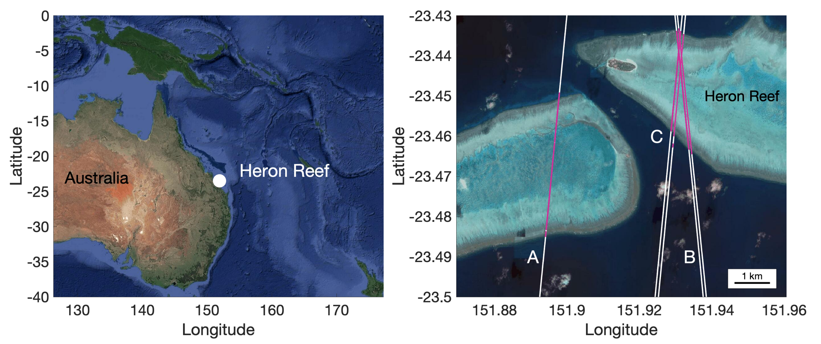
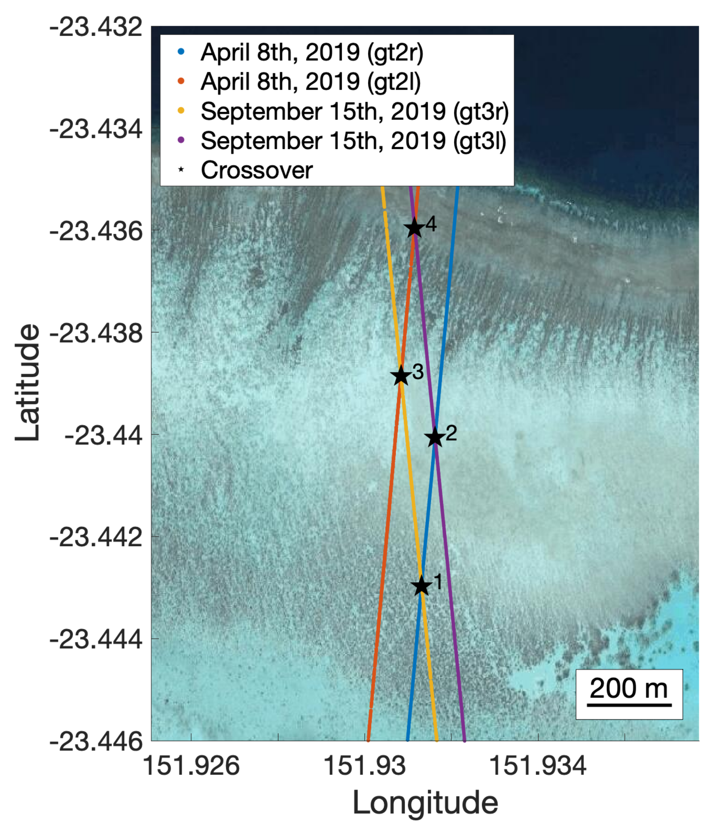
This section describes the two study areas and the different data sets included in this study as well as the methods needed to derive the ICESat-2 bathymetry.

2.1. Heron Reef

The Heron Reef (23 ° 27 S, 151 ° 55 E) in Queensland, Australia was used as one of the primary development sites for the algorithm due to its clear waters and the availability of accurate, high-resolution SDB data from EOMAP GmbH & Co. KG. The Heron Reef is a part of the Great Barrier Reef in Australia, and is located 70 km northeast of Gladstone, Queensland. The reef surrounds Heron Island, which is just 800 m wide. The average water temperature is around 25 ° C according to hourly temperatures listed by the AIMS Temperature Logger Program [16] and the salinity can be approximated to 35‰ by viewing at the AIMS eReefs Visualisation Portal (https://ereefs.aims.gov.au/ereefs-aims (accessed on 8 April 2021) [17].

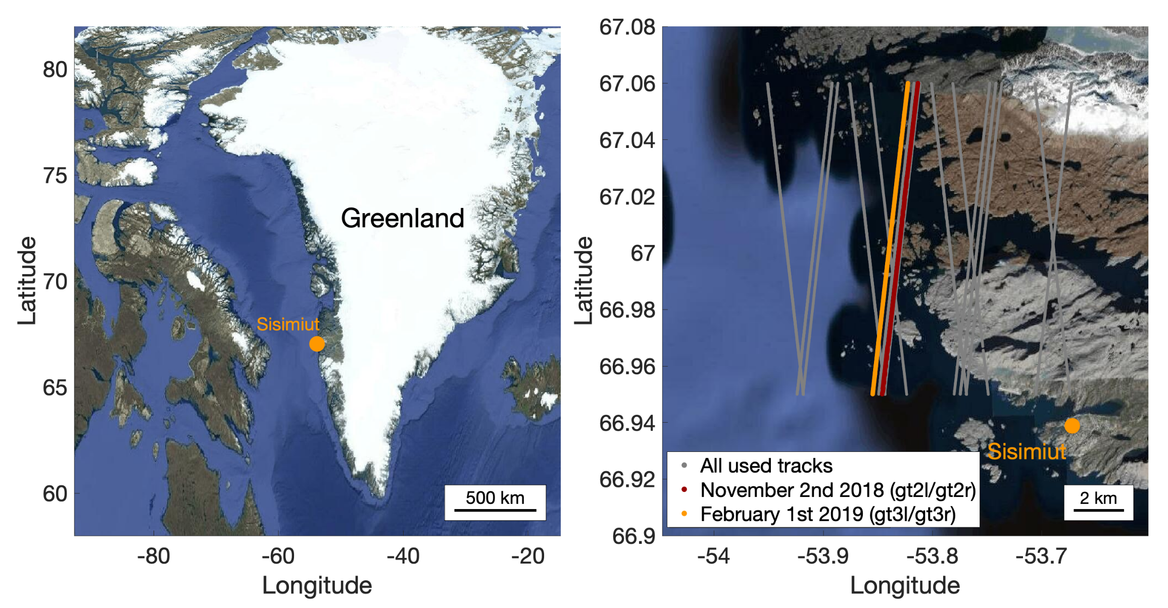
2.2. Sisimiut, Greenland

The coastal waters north-west of Sisimiut, Greenland were chosen as a validation site, to see how well ATLAS captures the bathymetry in the archipelago. It is located in the central-western coast of Greenland at 66 ° 56 20 N, 53 ° 40 20 W, around 320 km north of Nuuk. It is predominantly rocky seabed and with highly varying depths ranging from very deep (down to approximately 200 m) to very shallow areas (0–10 m). The coastal slopes are very high which is a challenge when measuring the depths. Between the skerries, there are patches of shallow water, where soundings by ship is more difficult to obtain.

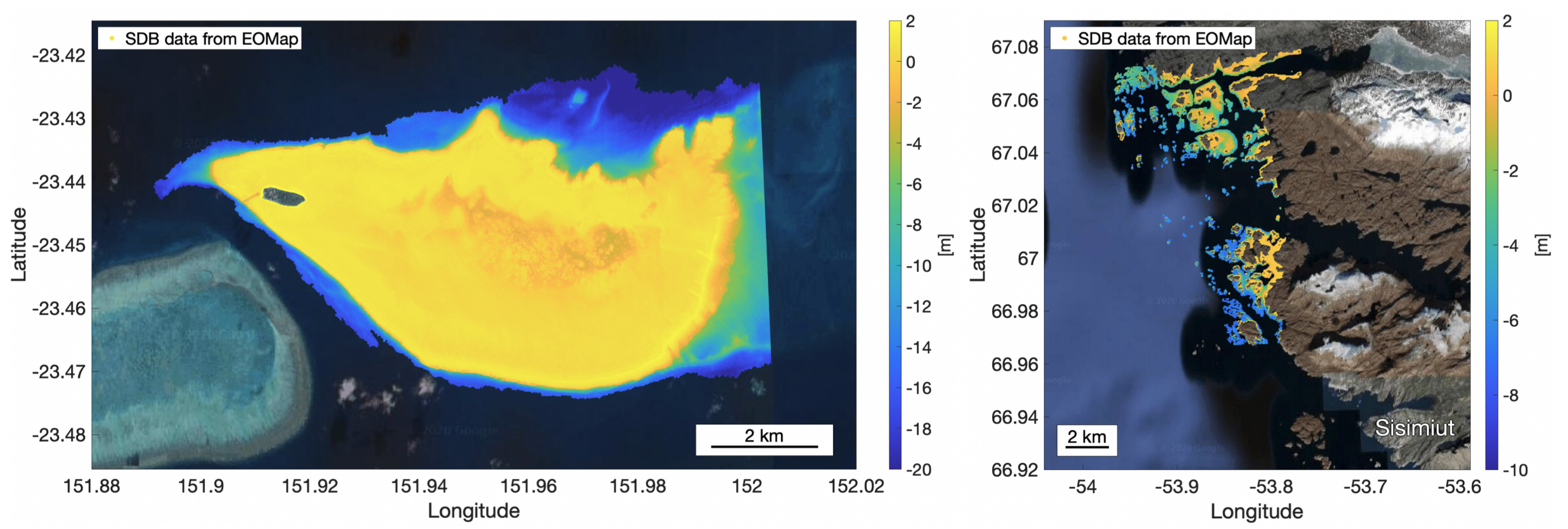
2.3. Satellite Derived Bathymetry from EOMAP

In order to evaluate the derived bathymetry from ICESat-2, SDB products from EOMAP GmbH & Co. KG have been used. Here we use SDB data for two areas: (1) Heron Reef in the Great Barrier Reef in Australia and (2) the area around Sisimiut, Greenland. The latter was provided by EOMAP in cooperation with the Danish Geodata Agency. Both data sets can be seen in Figure 1.
Derivation of SDB data is based on the semi-analytical model by [18,19] which is a remote-sensing reflectance model for shallow waters that do not require any in situ depth measurements. The model retrieves water depths, in addition to optical properties of the water and seabed, from above surface multispectral satellite measurements. The SDB product depends on water clarity and the seabed conditions, and typically only retrieves depths around 0–30 m.
According to the Survey Report attached to the demo data from the Heron Reef, EOMAP applies a physics-based procedure, where satellite data are corrected for adjacency from land as described in [20] and corrected for atmospheric and sea surface impacts according to [21]. The process is known as Modular Inversion Program (MIP) and a more thorough description can be found in several scientific articles [21,22,23]. For this study, both SDB data sets are based on the commercial optical satellite data from the Maxar/DigitalGlobe WorldView-2/3 sensor, which has a high spatial resolution of 2 m. For the Heron Reef, the provided SDB estimates have uncertainties between 0.5 and 2.6 m, or more specifically 0.5 m + 10% of the depth estimate, meaning that the uncertainty increases with depth. The uncertainties for the depth estimates are higher around Sisimiut, where they are based on comparisons with other reference data, and range between 40 cm and 2.4 m, with a mean value of 0.68 m, for depths down to 8 m. Here, the uncertainty also increases with depth. In the area around Sisimiut, the data set was originally referenced to the Lowest Astronomical Tide (LAT); however, using the DTU18LAT latoid model [24] and the EGM2008 geoid heights [25], the data were referenced to EGM2008 to ensure proper comparison between the different data sets. For the Heron Reef, the heights were relative to the mean sea level, and were adjusted using the DTU18MSS. No other adjustments or corrections were applied to these data.

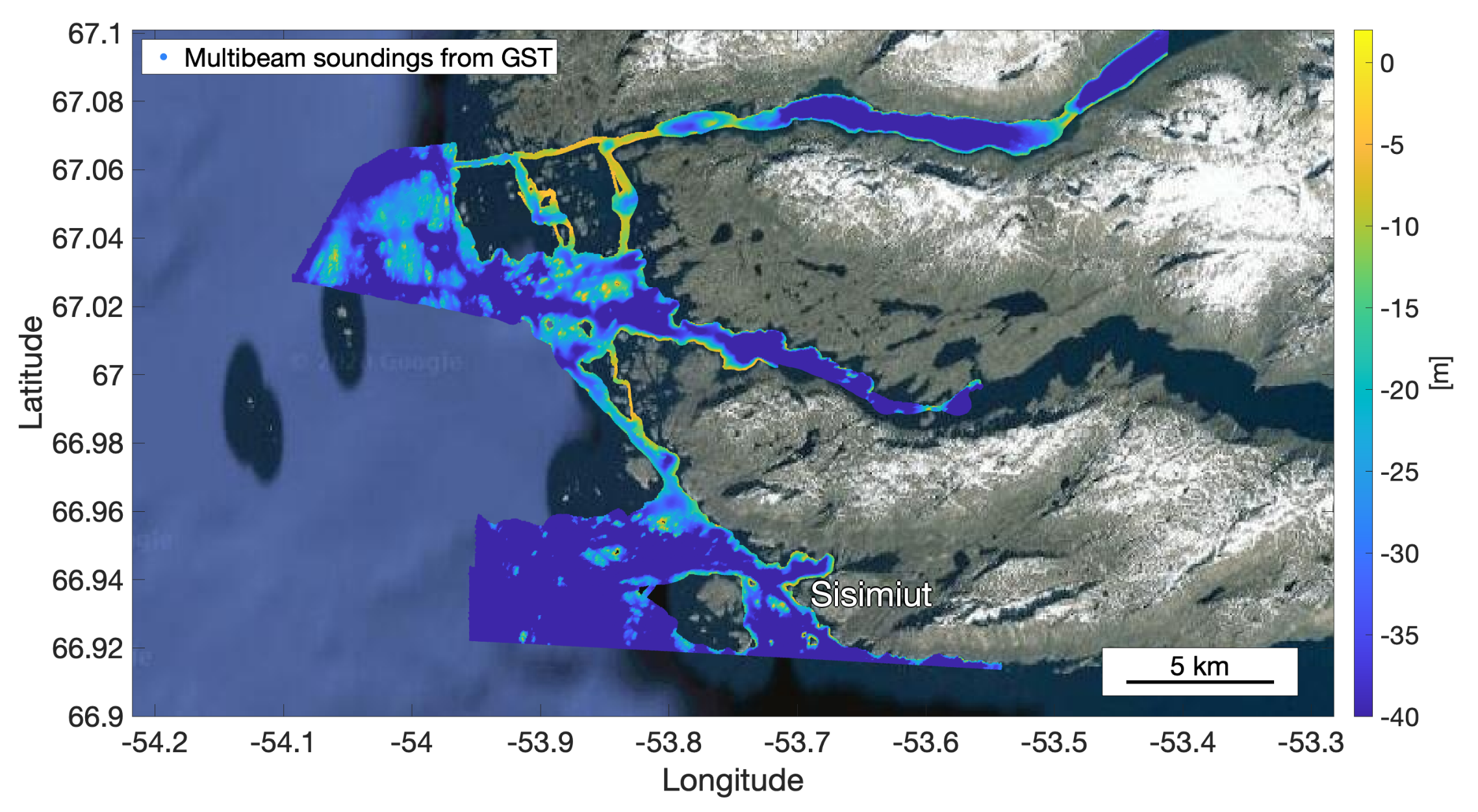
2.4. Multibeam Reference Data
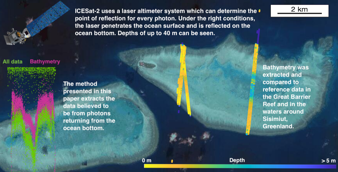
Around Sisimiut, multibeam reference data (see Figure 2) was collected by multibeam echo sounder (MBES) and delivered by the Danish Geodata Agency in cooperation with the surveyors from the Danish Defence. It was collected in the years 2012–2018 and the multibeam surveys are categorized with IHO order 2 [26], which is the least stringent order of hydrographic surveys as defined by the International Hydrographic Organization. The data set has a spatial resolution of 10 m within the surveyed areas. The depths were originally referenced to the lowest astronomical tide, but using the DTU18LAT latoid and the EGM2008 geoid, the bathymetry was referenced to the EGM2008 geoid instead. The time of ICESat-2 data capture and the collected multibeam will be different and therefore temporal changes may be present; however, such changes are expected to be small due to a predominantly rocky seabed in the areas of investigation.

2.5. ICESat-2 Data

ICESat-2 was launched by NASA on 15 September 2018 with the primary focus of monitoring elevation changes in the cryosphere. However, due to the green laser onboard the satellite, it is possible to map shallow ocean and lake bathymetry. The satellite carries a single instrument; the Advanced Topographic Laser Altimeter System, which is an altimeter using a green laser with a wavelength of 532 nm—meaning that the laser beam has a footprint size of around 17 m at the surface. ATLAS emits 10.000 laser pulses per second, corresponding to an along-track interval of 70 cm, and each pulse contains around 20 trillion photons. The photons travel with the speed of light towards the ground, where they are reflected. Some of the photons are reflected in the atmosphere and some on the surface. The number of reflected photons that returns to ATLAS depends on the reflectivity of the surface. For ice and snow, which are highly reflective, the number of photons that returns is around 10 per laser shot. For open ocean, which has a lower reflectance, the signal rate is around 0–4 [27]. Some of the photons also penetrate water surfaces and are reflected from either the water column or the bottom of the water body. If the water body is clear and calm, more photons will be reflected from the bottom. Muddy waters or waves limit the laser’s ability to reach the bottom as more photons are reflected higher in the water column.
The beams are pairwise arranged with 3.3 km between each pair. Within each pair there is a strong and a weak beam with 90 m distance. This setup makes it possible to determine an across-track surface slope, and for bathymetry purposes it facilitates the derivation of up to six different bathymetry profiles depending on the water clarity and other environmental characteristics that can affect the reflectance. The orbit of ICESat-2 has a repeat period of 91 days and an inclination of 92 degrees, and therefore provides data up to 88 degrees north and south. For the first two years, ICESat-2 was operating in a vegetation mapping mode, where the ground tracks were non-repeating on midlatitudes (<60°N/S). [28]
For this study we use the ATL03 level 2 product (version 3) [29], which contains data from the geolocated photons. The data can be downloaded for free (https://search.earthdata.nasa.gov/search) (accessed on 8 April 2021) and is stored in an easily read Hierarchical Data Format (HDF). For every single photon that is detected by ATLAS, a position is calculated and provided as longitude, latitude, and the height relative to the WGS84 ellipsoid. The ATL03 product includes everything necessary to derive the bathymetry profiles. The photon heights in the product have already been corrected for the necessary atmospheric effects and solid earth deformation, but also provides an ocean tide correction as well as the dynamic atmospheric correction, both of which are not automatically applied and will not be applied for this study. The along-track resolution of the ATL03 product is around 0.7 m. Using the provided geoid values, the heights are referenced to the EGM2008 geoid. The full ATL03 data dictionary can be obtained through the NSIDC webpage: https://nsidc.org/sites/nsidc.org/files/technical-references/ICESat2_ATL03_data_dict_v003.pdf (accessed on 8 April 2021).
For comparison, the bathymetry estimates from the ATL13 product are also shown in this study [30]. The main focus of the ATL13 product is on the inland water bodies; however, additional information is given about the depth of coastal waters. These bottom topography profiles are also derived from the ATL03 data. The ATL13 bathymetry is estimated using an empirical method described in [31].

2.6. Extracting Bathymetry Signals

The steps taken to identifying the bathymetry signals are described below. For the tuning of the algorithm tracks crossing various shallow waters were used. Since the water clarity and weather is more favourable at low latitudes with calm water, the development was undertaken looking at latitudes below 30 degrees N/S, where the best bathymetric reflections were encountered. Sites include Sharm El Sheik, Great Barrier Reef, Bermuda, Puerto Rico, etc.
Before applying an algorithm to detect the bathymetry, the land and sea surface reflections have to be removed from the data set. This is done using the following steps:
  • All ATL03 photons with heights, H, above 5 m (referenced to the geoid) are removed. This is done to remove the majority of photons reflected by islands and the coast.
  • The median height, H m e d i a n , of all the remaining data points is found. In ocean tracks, this median will be very close to the sea surface, once the heights above 5 m have been removed as done in the first step. While the laser can penetrate the air/water interface, most of the reflections are from the sea surface and they therefore dominate the median height.
  • After finding the median height, i.e., the sea surface, only data below this median are used onward. The algorithm uses a buffer, H b u f f to account for sea surface reflections below the median height. Data points are only kept if they fulfil H < ( H m e d i a n H b u f f ) . At low latitudes, where the algorithm has been used in coral reefs, the buffer was set to 0.5 m. However, at high latitudes, the buffer had to be higher due to a less distinctive sea surface, i.e., waves and more scattering near the surface, and was set to 1 m. The size of the buffer was chosen manually after studying several tracks in different locations. More automatic methods were also attempted using various filters and moving standard deviations of the surface photons to set size of the buffer. However, due to various signals caused by different sea states and near-surface bathymetry/topography, such automatic methods often failed and did not improve the end result but only added to the complexity of the algorithm.
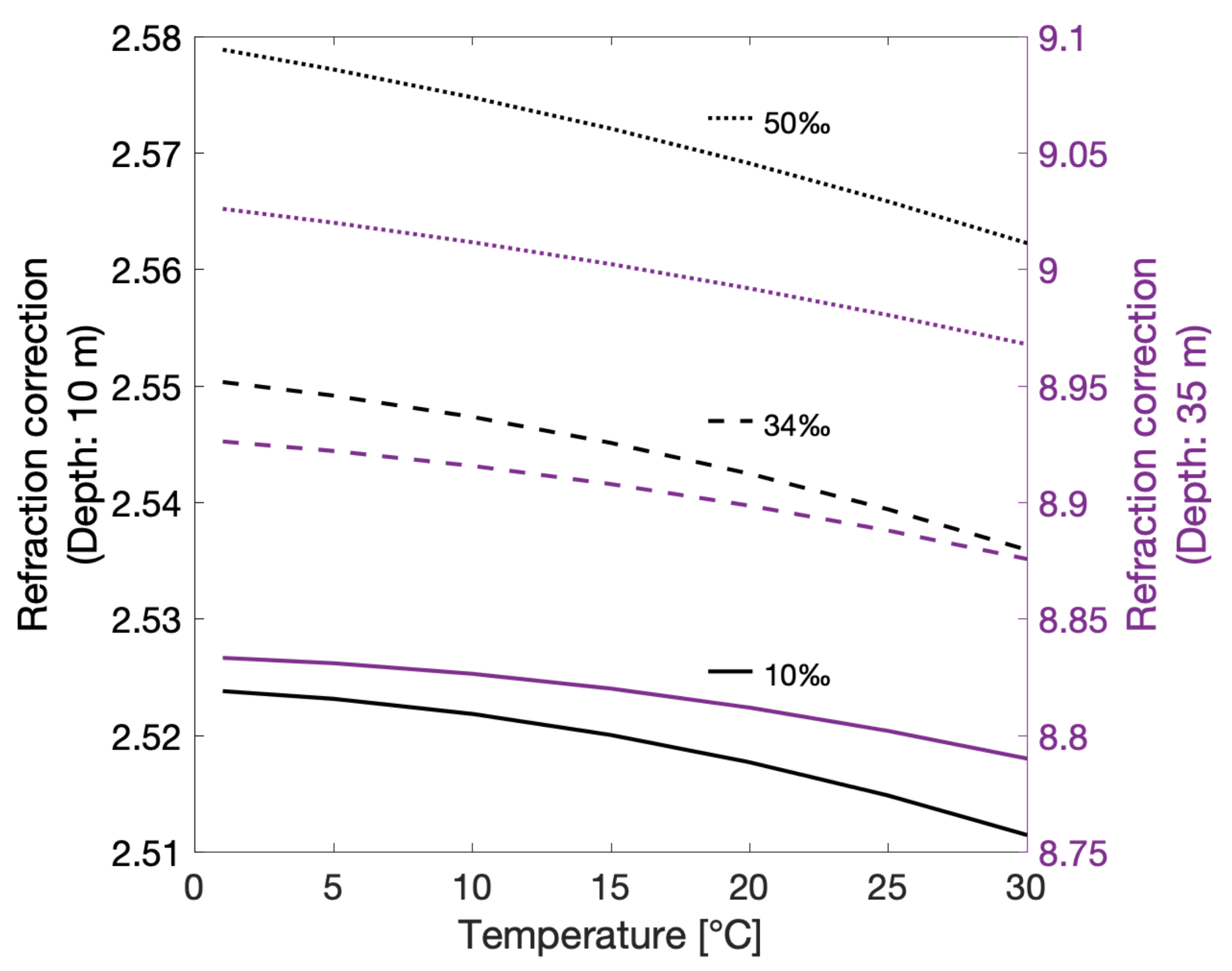
  • All subsurface data are then corrected for refraction at the air-sea interface using the method described in Section 2.7.
An example of how the discrimination between sub-surface and sea surface photons works is shown in Figure 3. Once the sub-surface photon data have been found, the bottom topography, if detected by the photons, can be found. The figure also shows the magnitude of the refraction correction.
5.
A moving median with a window of 50 data points is calculated, and data more than 3 m away from this are removed.
6.
Another moving median is calculated, this time using a window size of 30 points, resulting in H s m o o t h . A moving standard deviation of the difference between this and each data points is calculated as well.
7.
Now, the data are divided into three groups: High, medium and low confidence bathymetry. Outliers are once again excluded, but this time using different thresholds. First, indexes for data within a distance, k d i f f , of the just calculated moving median are found (see Equation (1)). The data within this distance and also with a moving standard deviation lower than k s t d are kept for further processing (See Equation (2)). Notice that the original heights are kept, whereas the smoothed heights are only used for finding the assumed bathymetry signals. The thresholds, k d i f f and k s t d , are stated in Table 1 and were determined by studying the bathymetry signals of several tracks around the Heron Reef, Australia, the Red Sea, Egypt, and the Maldives.
i x = | H s m o o t h H | < k d i f f ,
H k e e p = H [ i x & m o v s t d < k s t d ] .
8.
Then, the data are divided into segments dependent on latitude. Each segment has a length of 0.001 degrees latitude, which corresponds to an along-track distance of roughly 100 m. For each segment it is determined how many data points lie within each segment for each confidence (low, medium, high). If there are less than 10 data points within a segment, the data are not considered as bathymetry data. This limit was found most appropriate for a number of different tracks, but is chosen empirically and the limit might be better suited for some tracks compared to others. The limit is introduced to make sure that there are enough photons left to believe that an actual bathymetry signal has been detected.

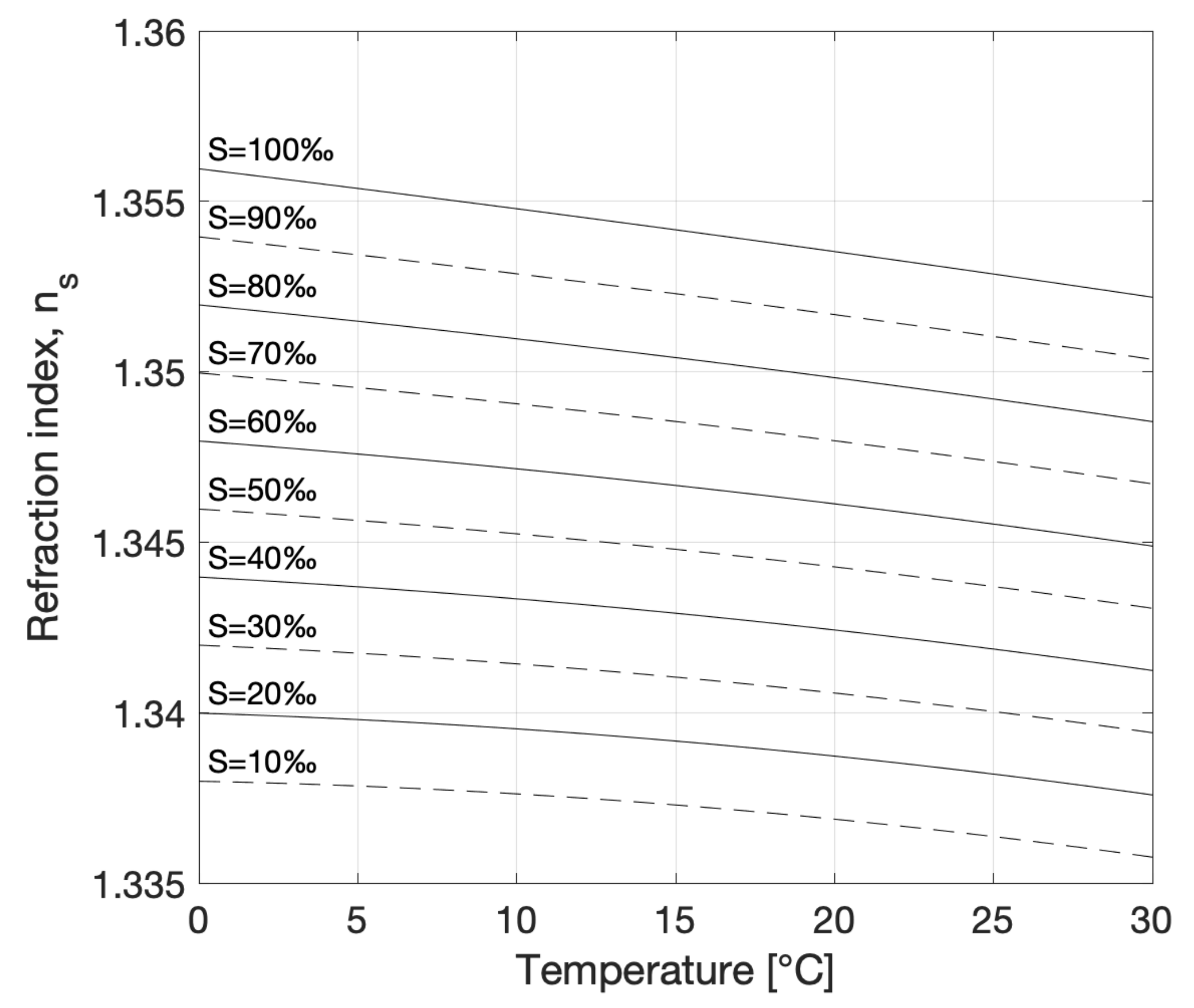
2.7. Refraction Correction

The photons from ATLAS are refracted in the air–water interface when they enter the ocean and continue their travel in the water. Once in the sea water, the photons travel at a lower speed and have changed direction. The refraction therefore introduces both a horizontal and a vertical offset compared to the geographical positions given in the ATL03 product. The positions given in the product assumes that the photon only travels in air, meaning that the distance travelled by the photon will be overestimated, making the bottom topography look deeper. In order to account for the refraction, some corrections must be applied. An illustration of the refraction is shown in Figure 4.
In [8] an approximation to the refraction correction for the vertical offset is introduced as Z = Z + 0.25416 D , where Z is the corrected photon height, Z are the original height measurements and D is the absolute depth from water surface to seafloor (see Figure 4). To obtain this approximation, they used a refractive index of 1.34116 based on water with a temperature of 20 °C, a salinity of 35 PSU, and a wavelength of 540 nm. The approximation is sufficient at lower latitudes, where the temperature is similar, but at higher latitudes, the approximation will lead to errors of around 1 cm at a depth of 10 m and 5 cm at a depth of 35 m. These numbers might be relatively small compared to the total error of the bathymetry estimate, but it was still decided to use a higher accuracy solution, also described by [8], which takes into consideration the refractive indices of air and water, n a i r and n s e a , the angle of incidence and azimuth of the unit pointing vector for the photon. The latter two parameters can be estimated by using the r e f _ e l e v and r e f _ a z i m u t h parameters available in the ATL03 file. The full derivation of the equations used can be found in [8]. For this study, we implement Equations (1)–(11) from [8] to calculate both the vertical and horizontal corrections.
The refractive index of water varies depending on the temperature and the salinity of the water as well as the wavelength of the laser beam. The approximated vertical correction is based on these numbers, and will work sufficiently in areas with similar conditions. However, if the water is significantly different, and if the horizontal offset is also needed, the full corrections to the measurement should be carried out. For this study, we are looking at ICESat-2 data in the area of Sisimiut, Greenland, where the average water temperature and salinity is very different from the 20 °C used in the approximation. According to the observations published in [32] the average water temperature from 1946 to 2013 was 1.67 °C for the top 50 m, and the corresponding mean salinity was 33.46‰. Therefore, it was chosen to use the full correction described in [8]. Firstly, the refractive index of sea water was calculated with values appropriate for the study areas. Ref. [33] presented an empirical function, where the water temperature, salinity and the photon wavelength is used to calculate the refraction index of water. Using the ATLAS wavelength of 532 nm, the empirical function simplifies to:
n s e a = n 0 + ( n 1 + n 2 T + n 3 T 2 ) S + ( n 4 + n 5 T ) T
where n 0 = 1.336 n 1 = 1.996 × 10 4 , n 2 = −1.050 × 10 6 , n 3 = 1.600 × 10 8 , n 4 = −7.951 × 10 6 , and n 5 = −2.020 × 10 6 are empirical constants and S and T are the local salinity and temperature, respectively. The equation above is applicable globally, as long as a temperature and salinity are provided as input.
Using this function and the temperature and salinity for Sisimiut yields a refraction index of 1.3426. Figure 5 shows the calculated refraction index of various temperatures and salinities and Figure 6 shows the corresponding vertical refraction corrections as a function of temperature using the equations from [8] with n s e a for three different salinities and a temperature ranging from 0 to 30 ° C. The lowest shown salinity of 10‰ corresponds to places such as the Baltic Sea with a sea surface salinity just below 10‰ [34], and salinities higher than 100‰ is usually only found in salt lakes, such as Lake Urmia in Iran [35]. The Gaet’ale Pond in Ethiopia currently holds the record as the most saline water body in the world with a salinity of 433‰ [36]. The effect of the refraction correction can be seen in Figure 3, where an example of uncorrected and corrected photon bounce points is shown.

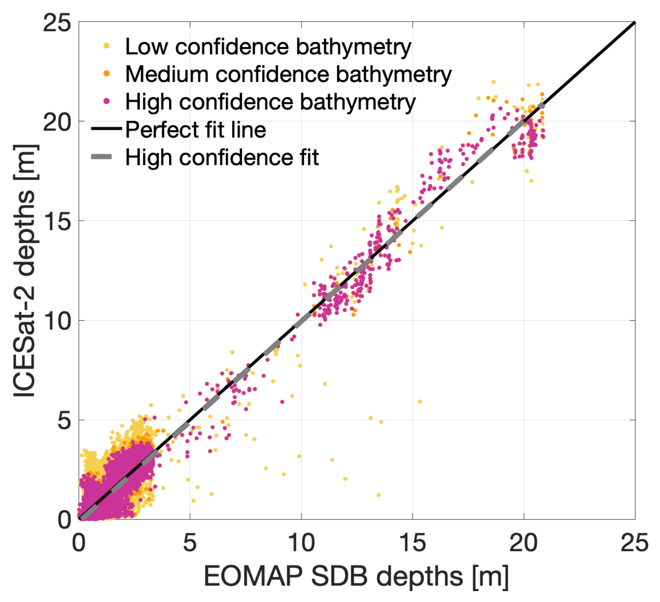
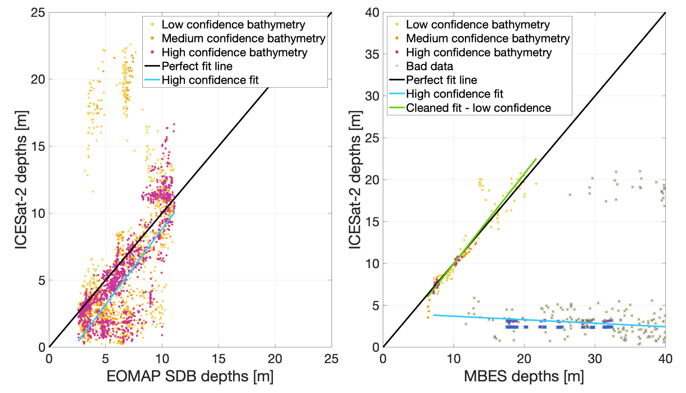
2.8. Comparison with Other Data Sources

Since the bathymetry will be described as a height above the EGM2008 geoid and all the in situ data sets have already been referenced to static reference surfaces, such as the latoid, we will not be making any corrections for tidal effects for this paper. The instantaneous depth from the ICESat-2 ATL03 data will be referenced to the EGM2008 geoid. Whenever the term “depth” is used, this will as such be with respect to the EGM2008 geoid and not the instantaneous sea surface.
The different reference data sets are interpolated to the positions of the photon reflections using a natural neighbour interpolation method without extrapolation to areas where there are no data. The natural neighbour interpolation is expected to perform well even if the query points are located at the boundary of the interpolated data set, since this kind of interpolation is computed using area based weights [37].
After interpolation of the reference data sets, the ICESat-2 bathymetry is compared to these by studying the median and mean absolute deviations, as well as the standard deviation of the differences, the RMSE and Pearson correlation coefficient.
The RMSE error was calculated as follows:
R M S E = 1 N 1 i = 1 N ( d i I S 2 d i ) 2
where N is the number of identified bathymetric photons from ICESat-2, d I S 2 is the depth below the geoid for each bathymetric photon, and d is the corresponding value from either SDB or MBES.
The Pearson correlation coefficient, ρ ( d I S 2 , d ) , is also found as the covariance divided by the product of the standard deviations, σ , of the two data sets:
ρ ( d I S 2 , d ) = c o v ( d I S 2 , d ) σ I S 2 σ
The above-mentioned statistics are calculated separately for each bathymetric confidence for all beams available in the studied region.

3. Results

Using the algorithms described in Section 2.6, the bathymetry signals from the ATL03 products were extracted for ICESat-2 passes over the Heron Reef in Australia as well as the waters near Sisimiut, Greenland.
To compare with the previously published method suggested by [9], the bathymetry signals obtained from an ICESat-2 track crossing the Yongle Atoll in China on 22 October 2018, is shown in Figure 7. Comparing the results from the high confidence bathymetry derived using the algorithm presented here to their results for the same track, the algorithm presented here performs just as well, if not better, as there are fewer outliers surrounding the bathymetry signal and less noise close to the surface.

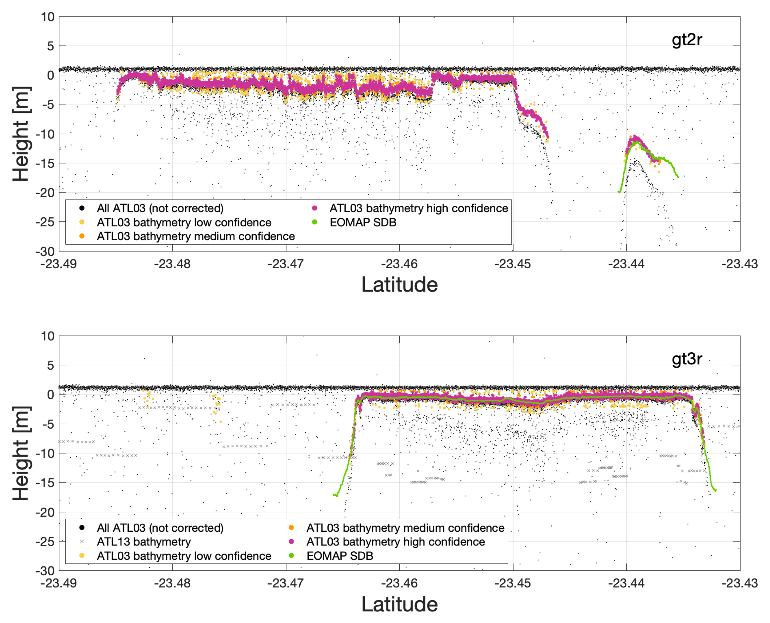
3.1. Heron Reef, Australia

Using a salinity of 35 and a sea temperature of 25 °C the bathymetry profiles were extracted for four different ICESat-2 tracks flying over the Heron Reef. The results for a selected couple of the beams from the overflight on 15 September 2019, are shown in Figure 8. For reference, the location of the different beams can be seen in Figure 9.
In total, four ICESat-2 overflights with a total of 15 beams crossing the Heron Reef were used for a statistical comparison. The bias between the ICESat-2 and SDB datasets can be seen in Figure 10. As seen from the figure, the ICESat-2 and SDB bathymetries agree very well with a small tendency of ICESat-2 depths to be higher below 15 m. The histogram in Figure 11 shows the distribution of the absolute differences between the ICESat-2 high confidence bathymetry photons and the corresponding SDB depths. The median and mean absolute deviations between the heights are shown in Table 2, along with the standard deviations and the RMSE. From these, it is clear that the higher the confidence, the better the ICESat-2 derived bathymetry agrees with that from SDB. The ATL13 product does not capture the bathymetry, and the GEBCO model, although closer to the observed bathymetry, has a very poor resolution.
Some of the tracks crossing the Heron Reef intersect and can be compared. This is the case for the beams shown in Figure 12. In total, four crossovers were compared in this area, between beams gt2r/gt2l and gt3r/gt3l from 8 April 2019, and 15 September 2019, respectively. The heights at intersections as well the absolute differences are given in Table 3. Without smoothing the data sets, but simply by using linear interpolation to the point of intersection, the median absolute difference between the different bathymetry estimates was found to be 15 cm. When first smoothing the data with a Gaussian weighted moving average with a window size of 20 points, the median absolute difference was 2 cm. The 15 cm are well within the expected error margin, and without smoothing one would not expect this value to be smaller, also because the bathymetry in coral reefs varies a lot over very short distances. It is worth noting that crossover point no. 2, which is the one with the biggest discrepancies, is also the intersect of two weak beams, whereas crossover point no. 3, which has the smallest difference, is the intersection of two strong beams.

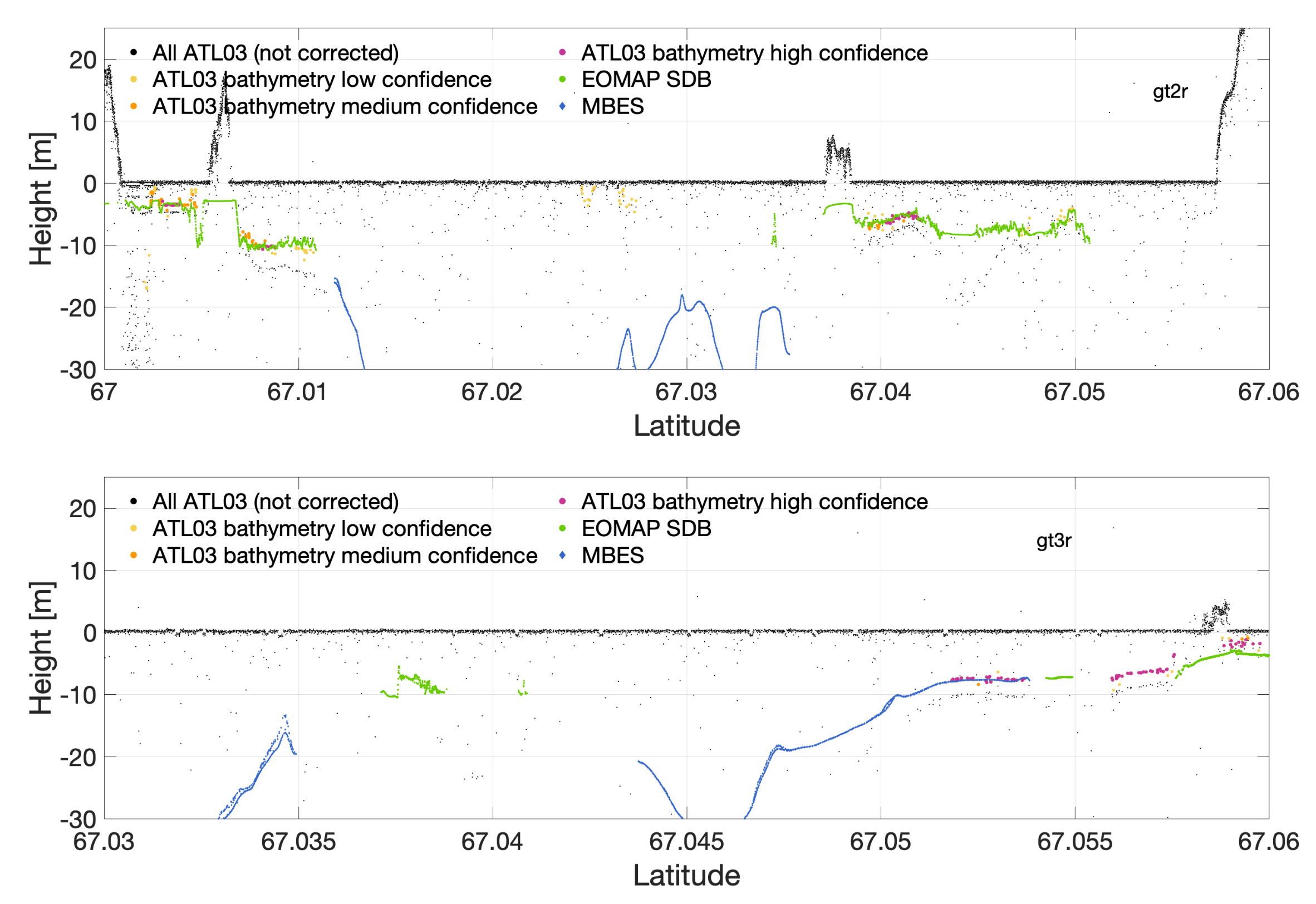
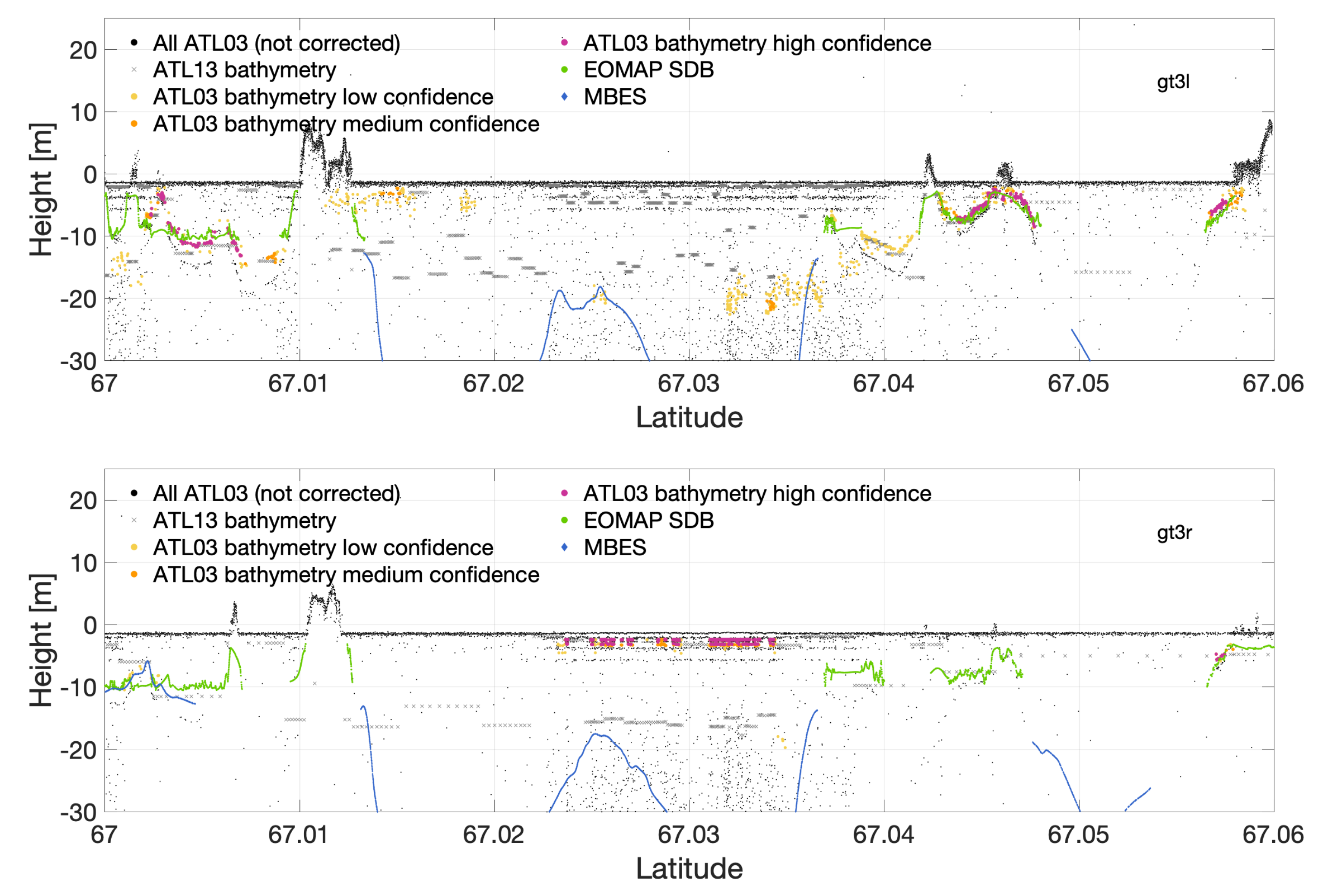
3.2. Sisimiut, Greenland

The algorithm described in Section 2.6 was also used to extract bathymetry profiles at higher latitudes near Sisimiut, Greenland. The tracks studied in this area are shown in Figure 13.
The results for beams gt2r and gt3r from a track crossing the area on 2 November 2018, are shown in Figure 14. For beam gt2r, it can be seen that the extracted bathymetry agrees well with the SDB data from EOMAP and the MBES data (see latitudes between 66.99 and 67.0°N). However, for the most part, the MBES bathymetry is available for depths that cannot be reached by the ATLAS photons or from satellite imagery. The visibly thicker line for the GEBCO model shown in the bottom part of Figure 14 around 67.04 ° N is merely a result of the visualisation and the fact that a nearest neighbour interpolation was used for the GEBCO values.
A more mixed result was obtained when the ICESat-2 satellite flew over the same area on 1 February 2019, see Figure 15. The data from beam gt3l show that the extracted bathymetry is very similar to that obtained from satellite imagery. Even a bathymetric signal with a depth of more than 10 m is captured by ICESat-2 around 67.04 degrees north. The extracted signals for beam gt3r are not from bathymetry, but are interpreted as bathymetry by the algorithm because of the high density of signal returns coming from these depths. The same lines also appear in the gt3l data, but here, the density of the deeper reaching photons is higher and the moving median is therefore placed at higher depths. For both the gt3l and gt3r data, the ATL13 product mistook these lines as bathymetry.
The left plot in Figure 16 shows the bias between SDB and the bathymetry derived from ICESat-2. Compared to the observed bias for the data from the Heron Reef, the bias is larger in the area around Sisimiut. There does not seem to be a pattern to describe this, and the discrepancies are most likely just a result of the inaccuracies of both methods in these Arctic waters.
When comparing ICESat-2 bathymetries with the MBES data set (right plot in Figure 16), it can be seen that the proposed algorithm wrongly assumes that mirror reflections in the top 5 m of the ocean are caused by bathymetry, when actually, the true ocean bottom is beyond measure for photons. If the obvious misinterpretations are removed by only including data points where the absolute difference between MBES and ICESat-2 bathymetry is less than 7 m, it can be seen that the ICESat-2 bathymetry agrees well with the MBES data. Unfortunately, this exclusion of bad data leaves behind only a small amount of bathymetry data. The statistics resulting from a comparison between the three kinds of bathymetry can be seen in Table 4. As seen, the numbers are not as convincing as they were in the Heron Reef. However, to methods relying on light reflection (such as lidar and SDB), the area around Sisimiut is also more challenging compared to the coral reefs in Australian waters. The correlation between SDB and ICESat-2 is present, but the deviations are around 2 m without a clear reason such as was the case for the MBES comparison. The statistics between ICESat-2 and MBES bathymetry are based on small numbers, but an agreement is definitely visible.

4. Discussion

Overall, the bathymetry from ICESat-2 derived from using the method proposed in Section 2.6 agrees well with other available bathymetry data sets. Good results were seen especially for the Heron Reef, Australia, where the waters are clear and the ocean bottom is sand and corals. In this area the ICESat-2 bathymetry was compared to SDB depths provided by EOMAP, and the median deviation between the ocean bottom topography estimates was less than 20 cm. In the area around Sisimiut, ICESat-2 data were compared to both an SDB and a MBES dataset. In this area, the ICESat-2 data were more ambiguous causing the proposed method to misinterpret certain photon bounces as being from the seabed while they were in fact mirror reflections in the surface waters in areas where the ocean bottom was at too great depths for the photons to reach and thereby for ATLAS to detect any reflections. In [8] they calculated RMSEs between ICESat-2 bathymetry and airborne lidar data to be around 43 to 60 cm near St. Thomas, U.S. Virgin Islands. The RMSEs found in this study, for the Heron Reef, Australia, range between 28 and 45 cm. However, the maximum depth in this area is only around 22 m, whereas the bathymetry found near St. Thomas in [8] covered depths all the way down to 38 m.
ICESat-2 and SDB only applies to shallow waters while the MBES data also used in this study mainly measure bottom topography at greater depths. This resulted in very little overlapping data between ICESat-2 and MBES in the area around Sisimiut. Therefore, it would be preferable to get more tracks with data in order to perform a better analysis. However, as the validity of ICESat-2 bathymetry has already been proven in other publications [8,9,10], the main goal of this study is to present a method that automatically detects photons reflected from the shallow ocean bottom. The results from this study show that the method presented in Section 2.6 is able to extract most bathymetric signals from the geolocated photon data. The empirical method will perform better or worse for different tracks depending on the thresholds and window sizes used for the different steps. As such, the algorithm can be adjusted to a specific region to obtain better results. Here it was chosen to keep as many thresholds as possible the same for all situations. Therefore, only the buffer below the estimated sea surface varied to accommodate the different sea states. The approach is challenged by the inability of statistics to differ between noise and bathymetry, when the density of the noise is equal to the density of the bathymetry signals. This has proven to be difficult especially in deep waters, where patches of very calm waters can lead to multiple mirror reflections in the shallow part of the water column. These could be filtered out by only looking at bathymetry at depths beyond 5 m; however, this would also result in a huge loss of the shallow bathymetry caught by the algorithm. Misinterpretations are also seen when the appearance of the sea surface is affected by waves or land.
The ATL03 product also includes an estimation of the height uncertainty (1− σ ) for the consecutive reference photons for which all geophysical corrections are provided. The provided uncertainty estimate includes many effects such as those of electronics timing jitter, the transmit pulse width, radial orbit uncertainty, pointing angle uncertainty. In the area around Sisimiut the median uncertainty for all low confidence bathymetry photons is 63 cm, whereas it is only 23 cm for the high confidence photons. As expected, the height uncertainty is lower for the Heron Reef, with median values of 24 and 13 cm for the low and high confidence bathymetry photons. The uncertainties did not appear to depend on the depth of the bounce point.
There is also an error in the refraction correction linked to the way the local mean sea surface is computed, since the refraction correction depends on the depth of the assumed photon bounce. Here, we simply use the median of what we characterize as the surface photon returns, but in reality, the actual surface could be higher or lower, depending on local factors such as waves, sea spray, objects below the sea surface [38]. Another assumption that might lead to inaccuracies in the height estimates is the fact that a single value for the mean sea level for every beam track is used. The ideal sea level would be the instantaneous sea level observed by every single photon, as the sea surface varies from place to place due to waves, currents, and tides. An approach that accommodates this was used in [9], but was not implemented here. They estimated that the horizontal accuracy of the position of an underwater ICESat-2 photon is approximately 6 m [9], where 5 m were attributed to the above surface contribution [39] and the remaining error was assumed to be from refraction errors.
The algorithm presented in this study performs well overall. However, some challenges make it hard to use an empirical method near the air-sea interface, because very shallow topography can be hard to distinguish from sea surface reflections. Moreover, sometimes the noise density is as high as the signal density, in which case the empirical approach will fail, because it cannot tell a true signal from a false one. The bathymetry signals from ICESat-2 do not provide global coverage, but they offer a way to do regional studies, perhaps even to see change with time. The ICESat-2 data could also be used as an input for training SDB models and/or to verify these, such as is done in [9,10,11,12].
In conclusion, it can be said that the statistical approach presented here works well, even more so under supervision, to extract bathymetry signals locally or regionally, where one can do an intermediate evaluation. However, a more global extraction of bathymetry signals from the ICESat-2 ATL03 product should be approached with deep learning methods trained with known bathymetry.

Author Contributions

Conceptualization, H.R. and O.B.A.; Data curation, H.R., P.S.C. and O.B.A.; Formal analysis, H.R.; Funding acquisition, O.B.A.; Investigation, H.R.; Methodology, H.R.; Project administration, H.R.; Resources, O.B.A.; Software, H.R. and P.K.; Supervision, O.B.A.; Validation, H.R.; Visualization, H.R.; Writing—original draft, H.R., P.S.C. and P.K.; Writing—review & editing, H.R., P.S.C. and K.N. All authors have read and agreed to the published version of the manuscript.

Funding

This research was supported by the EOforChina DANIDA project (grant file number 18-M01-DTU).

Data Availability Statement

NASA’s ICESat-2 data can be downloaded from the NSIDC website. ATL03: https://nsidc.org/data/atl13/versions/3 (accessed on 8 April 2021) and ATL13: https://nsidc.org/data/atl13/versions/3 (accessed on 8 April 2021). EOMAP SDB Demo Data can be requested here: https://www.eomap.com/great-barrier-reef/ (accessed on 8 April 2021).

Acknowledgments

We thank the NASA National Snow and Ice Data Center (NSIDC) Distributed Active Archive Center (DAAC) for distributing the ICESat-2 data. We also thank EOMAP GmbH & Co.KG for providing their SDB data. We would also like to thank the anonymous reviewers for their comments and suggestions, which helped to improve this paper.

Conflicts of Interest

The authors declare no conflict of interest.

References

  1. Hamden, M.H.; Din, A.H.M. A review of advancement of hydrographic surveying towards ellipsoidal referenced surveying technique. IOP Conf. Ser. Earth Environ. Sci. 2018, 169, 012019. [Google Scholar] [CrossRef]
  2. Micallef, A. Chapter Thirteen—Marine Geomorphology: Geomorphological Mapping and the Study of Submarine Landslides. In Geomorphological Mapping; Developments in Earth Surface Processes; Smith, M.J., Paron, P., Griffiths, J.S., Eds.; Elsevier: Amsterdam, The Netherlands, 2011; Volume 15, pp. 377–395. [Google Scholar] [CrossRef]
  3. Tewinkel, G. Water depths from aerial photographs. Photogramm. Eng. 1963, 29, 1037–1042. [Google Scholar]
  4. Murase, T.; Tanaka, M.; Tani, T.; Miyashita, Y.; Ohkawa, N.; Ishiguro, S.; Suzuki, Y.; Kayanne, H.; Yamano, H. A photogrammetric correction procedure for light refraction effects at a two-medium boundary. Photogramm. Eng. Remote Sens. 2008, 74, 1129–1136. [Google Scholar] [CrossRef]
  5. Cao, B.; Fang, Y.; Jiang, Z.; Gao, L.; Hu, H. Shallow water bathymetry from WorldView-2 stereo imagery using two-media photogrammetry. Eur. J. Remote Sens. 2019, 52, 506–521. [Google Scholar] [CrossRef] [Green Version]
  6. Hodúl, M.; Bird, S.; Knudby, A.; Chénier, R. Satellite derived photogrammetric bathymetry. ISPRS J. Photogramm. Remote Sens. 2018, 142, 268–277. [Google Scholar] [CrossRef]
  7. Arsen, A.; Crétaux, J.F.; Berge-Nguyen, M.; Del Rio, R.A. Remote Sensing-Derived Bathymetry of Lake Poopó. Remote Sens. 2014, 6, 407–420. [Google Scholar] [CrossRef] [Green Version]
  8. Parrish, C.E.; Magruder, L.A.; Neuenschwander, A.L.; Forfinski-Sarkozi, N.; Alonzo, M.; Jasinski, M. Validation of ICESat-2 ATLAS Bathymetry and Analysis of ATLAS’s Bathymetric Mapping Performance. Remote Sens. 2019, 11, 1634. [Google Scholar] [CrossRef] [Green Version]
  9. Ma, Y.; Xu, N.; Liu, Z.; Yang, B.; Yang, F.; Wang, X.H.; Li, S. Satellite-derived bathymetry using the ICESat-2 lidar and Sentinel-2 imagery datasets. Remote Sens. Environ. 2020, 250, 112047. [Google Scholar] [CrossRef]
  10. Thomas, N.; Pertiwi, A.P.; Traganos, D.; Lagomasino, D.; Poursanidis, D.; Moreno, S.; Fatoyinbo, L. Space-Borne Cloud-Native Satellite-Derived Bathymetry (SDB) Models Using ICESat-2 And Sentinel-2. Geophys. Res. Lett. 2021, 48, e2020GL092170. [Google Scholar] [CrossRef]
  11. Babbel, B.J.; Parrish, C.E.; Magruder, L.A. ICESat-2 Elevation Retrievals in Support of Satellite-Derived Bathymetry for Global Science Applications. Geophys. Res. Lett. 2021, 48, e2020GL090629. [Google Scholar] [CrossRef]
  12. Albright, A.; Glennie, C. Nearshore Bathymetry from Fusion of Sentinel-2 and ICESat-2 Observations. IEEE Geosci. Remote Sens. Lett. 2021, 18, 9086432. [Google Scholar] [CrossRef]
  13. Goodrich, K.; Smith, R. ICESat-2 Space-Based Laser Validation for Satellite-Derived Bathymetry in NSF-Funded Research. Sea Technol. 2020, 61, 15–20. [Google Scholar]
  14. Fair, Z.; Flanner, M.; Brunt, K.M.; Amanda Fricker, H.; Gardner, A. Using ICESat-2 and Operation IceBridge altimetry for supraglacial lake depth retrievals. Cryosphere 2020, 14, 4253. [Google Scholar] [CrossRef]
  15. Fricker, H.A.; Arndt, P.; Brunt, K.M.; Datta, R.T.; Fair, Z.; Jasinski, M.F.; Kingslake, J.; Magruder, L.A.; Moussavi, M.; Pope, A.; et al. ICESat-2 Meltwater Depth Estimates: Application to Surface Melt on Amery Ice Shelf, East Antarctica. Geophys. Res. Lett. 2021, 48, e2020GL090550. [Google Scholar] [CrossRef]
  16. Australian Institute of Marine Science (AIMS). Sea Water Temperature Logger Data at Heron Island, Great Barrier Reef from 24 Nov 1995 to 18 Dec 2020; Technical Report. Available online: https://apps.aims.gov.au/metadata/view/446a0e73-7c30-4712-9ddb-ba1fc29b8b9a (accessed on 8 April 2021).
  17. Skerratt, J.; Mongin, M.; Baird, M.; Wild-Allen, K.; Robson, B.; Schaffelke, B.; Davies, C.; Richardson, A.; Margvelashvili, N.; Soja-Wozniak, M.; et al. Simulated nutrient and plankton dynamics in the Great Barrier Reef (2011–2016). J. Mar. Syst. 2019, 192, 51–74. [Google Scholar] [CrossRef]
  18. Lee, Z.; Carder, K.L.; Mobley, C.D.; Steward, R.G.; Patch, J.S. Hyperspectral remote sensing for shallow waters. I. A semianalytical model. Appl. Opt. 1998, 37, 6329–6338. [Google Scholar] [CrossRef] [PubMed]
  19. Lee, Z.; Carder, K.L.; Mobley, C.D.; Steward, R.G.; Patch, J.S. Hyperspectral remote sensing for shallow waters: 2. Deriving bottom depths and water properties by optimization. Appl. Opt. 1999, 38, 3831–3843. [Google Scholar] [CrossRef] [Green Version]
  20. Kiselev, V.; Bulgarelli, B.; Heege, T. Sensor independent adjacency correction algorithm for coastal and inland water systems. Remote Sens. Environ. 2014, 157, 85–95. [Google Scholar] [CrossRef]
  21. Heege, T.; Kiselev, V.; Wettle, M.; Hung, N.N. Operational multi-sensor monitoring of turbidity for the entire Mekong Delta. Int. J. Remote Sens. 2014, 35, 2910–2926. [Google Scholar] [CrossRef]
  22. Cerdeira-Estrada, S.; Heege, T.; Kolb, M.; Ohlendorf, S.; Uribe, A.; Muller, A.; Garza, R.; Ressl, R.; Aguirre, R.; Marino, I.; et al. Benthic habitat and bathymetry mapping of shallow waters in Puerto morelos reefs using remote sensing with a physics based data processing. In Proceedings of the International Geoscience and Remote Sensing Symposium, Munich, Germany, 22–27 July 2012; p. 6350402. [Google Scholar] [CrossRef]
  23. Siermann, J.; Harvey, C.; Morgan, G.; Heege, T. Satellite derived bathymetry and Digital Elevation Models (DEM). In Proceedings of the IPTC 2014 International Petroleum Technology Conference, Doha, Qatar, 19–22 January 2014; 2, pp. 1284–1293. [Google Scholar] [CrossRef]
  24. Andersen, O.; Stenseng, L.; Piccioni, G.; Knudsen, P. The DTU15 MSS (Mean Sea Surface) and DTU15LAT (Lowest Astronomical Tide) reference surface. In Proceedings of the ESA Living Planet Symposium, Prague, Czech Replubic, 9–13 May 2016. [Google Scholar]
  25. Pavlis, N.K.; Holmes, S.A.; Kenyon, S.C.; Factor, J.K. The development and evaluation of the Earth Gravitational Model 2008 (EGM2008). J. Geophys. Res. Solid Earth 2012, 117. [Google Scholar] [CrossRef] [Green Version]
  26. International Hydrographic Bureau. International Hydrographic Organization (2008) IHO Standards for Hydrographic Surveys; Technical Report; International Hydrographic Bureau: Monaco City, Monaco, 2020. [Google Scholar]
  27. Klotz, B.W.; Neuenschwander, A.; Magruder, L.A. High-Resolution Ocean Wave and Wind Characteristics Determined by the ICESat-2 Land Surface Algorithm. Geophys. Res. Lett. 2020, 47, e2019GL085907. [Google Scholar] [CrossRef]
  28. Markus, T.; Neumann, T.; Martino, A.; Abdalati, W.; Brunt, K.; Csatho, B.; Farrell, S.; Fricker, H.; Gardner, A.; Harding, D.; et al. The Ice, Cloud, and land Elevation Satellite-2 (ICESat-2): Science requirements, concept, and implementation. Remote Sens. Environ. 2017, 190, 260–273. [Google Scholar] [CrossRef]
  29. Neumann, T.A.; Brenner, A.; Hancock, D.; Robbins, J.; Saba, J.; Harbeck, K.; Gibbons, A.; Lee, J.; Luthcke, S.B.; Rebold, T. ATLAS/ICESat-2 L2A Global Geolocated Photon Data, Version 3. ATL03; NASA National Snow and Ice Data Center Distributed Active Archive Center (NSIDC DAAC): Boulder, CO, USA. [CrossRef]
  30. Jasinski, M.F.; Stoll, J.D.; Hancock, D.; Robbins, J.; Nattala, J.; Morison, J.; Jones, B.M.; Ondrusek, M.E.; Pavelsky, T.M.; Parrish, C. Algorithm Theoretical Basis Document (ATBD) for Inland Water Data Products, ATL13, Version 3, Release Date 1 March. 2020. Available online: https://nsidc.org/sites/nsidc.org/files/technical-references/ICESat2_ATL13_ATBD_r003.pdf (accessed on 8 April 2021).
  31. Jasinski, M.F.; Stoll, J.D.; Hancock, D.; Robbins, J.; Nattala, J.; Morison, J.; Jones, B.M.; Ondrusek, M.E.; Pavelsky, T.M.; Parrish, C. ATL13 Product Data Dictionary for Inland Water Data Products, ATL13, Version 3, Release Date 3 February 2020. 2020. Available online: https://nsidc.org/sites/nsidc.org/files/technical-references/ICESat2_ATL13_data_dict_v003.pdf (accessed on 8 April 2021).
  32. Ribergaard, M.H. Oceanographic Investigations Off West Greenland 2013; Technical Report; Danish Meteorological Institute, Centre for Ocean and Ice: Copenhagen, Denmark, 2013; Available online: http://ocean.dmi.dk/staff/mhri/Docs/scr14-001.pdf (accessed on 8 April 2021).
  33. Quan, X.; Fry, E.S. Empirical equation for the index of refraction of seawater. Appl. Opt. 1995, 34, 3477–3480. [Google Scholar] [CrossRef] [PubMed]
  34. Meier, H.E.M.; Kauker, F. Modeling decadal variability of the Baltic Sea: 2. Role of freshwater inflow and large-scale atmospheric circulation for salinity. J. Geophys. Res. Ocean. 2003, 108. [Google Scholar] [CrossRef] [Green Version]
  35. Sharifi, A.; Shah-Hosseini, M.; Pourmand, A.; Esfahaninejad, M.; Haeri-Ardakani, O. The Vanishing of Urmia Lake: A Geolimnological Perspective on the Hydrological Imbalance of the World’s Second Largest Hypersaline Lake; Springer: Berlin/Heidelberg, Germany, 2018; pp. 1–38. [Google Scholar] [CrossRef]
  36. Pérez, E.; Chebude, Y. Chemical Analysis of Gaet’ale, a Hypersaline Pond in Danakil Depression (Ethiopia): New Record for the Most Saline Water Body on Earth. Aquat. Geochem. 2017, 23, 109–117. [Google Scholar] [CrossRef]
  37. Amidror, I. Scattered data interpolation methods for electronic imaging systems: A survey. J. Electron. Imaging 2002, 11, 157–176. [Google Scholar] [CrossRef]
  38. Neumann, T.A.; Brenner, A.; Hancock, D.; Robbins, J.; Saba, J.; Harbeck, K.; Gibbons, A.; Lee, J.; Luthcke, S.B.; Rebold, T. Algorithm Theoretical Basis Document (ATBD) for Global Geolocated Photons ATL03, Version 3, Release Date 1 April 2020. 2020. Available online: https://nsidc.org/sites/nsidc.org/files/technical-references/ICESat2_ATL03_ATBD_r003.pdf (accessed on 8 April 2020).
  39. Neuenschwander, A.L.; Magruder, L.A. Canopy and terrain height retrievals with ICESat-2: A first look. Remote Sens. 2019, 11, 1721. [Google Scholar] [CrossRef] [Green Version]
Figure 1. (left) SDB bathymetry of Heron Reef wrt. to the mean sea level, and (right) north of Sisimiut, Greenland, wrt. the latoid.
Remotesensing 13 03548 g001
Figure 2. Multibeam echo sounding reference data in the area around Sisimiut, Greenland.
Remotesensing 13 03548 g002
Figure 3. Illustration of discrimination procedure using a track crossing Heron Reef on 15 September 2019 (beam gt1r). Surface points are shown in grey, with the median surface height in black, subsurface points before the refraction correction are shown in green. Blue points correspond to the subsurface data after the refraction correction.
Remotesensing 13 03548 g003
Figure 4. Illustration of refraction of the laser beams at the air-sea interface. Inspiration from [8].
Remotesensing 13 03548 g004
Figure 5. Refraction index for sea water at various salinities and temperatures. Only valid for the ATLAS instrument, which uses a green laser with a wavelength of 532 nm.
Remotesensing 13 03548 g005
Figure 6. Vertical refraction correction as a function of temperature for three different salinities and at two different depths of 10 m (left y-axis) and 35 m (right y-axis).
Remotesensing 13 03548 g006
Figure 7. ICESat-2 track crossing the Yongle Atoll in South China Sea on 22 October 2018. The beam shown in this plot is gt3r. (Top left) Location of the Yongle Atoll in the South China Sea, (Top right) Location of beam gt3r across the Yongle Atoll, and (bottom) the derived bathymetry signal compared to uncorrected ATL03 data.
Remotesensing 13 03548 g007
Figure 8. ICESat-2 track crossing Heron Reef on 15 September 2019. ICESat-2 data from ATL13 and ATL03 shown along with SDB data and the GEBCO model.
Remotesensing 13 03548 g008
Figure 9. (Left) Location of Heron Reef, Australia. (Right) Map of ICESat-2 tracks, pink highlights areas with detected bathymetry. A: 8 April 2019, beam gt3l (strong), B: 15 September 2019, beams gt3l/gt3r(strong), C: 8 April 2019, beams gt2l/gt2r(weak).
Remotesensing 13 03548 g009
Figure 10. Bias plot comparing the depth of Heron Reef, Australia from ICESat-2 and EOMAP. Depths are metres below the EGM2008 geoid. A perfect fit line (black) is shown along with a linear fit of all high confidence data (grey).
Remotesensing 13 03548 g010
Figure 11. Histogram showing the absolute differences between ICESat-2 and EOMAP depth estimates for Heron Reef, Australia.
Remotesensing 13 03548 g011
Figure 12. Crossover points over Heron Reef between two beam pairs from tracks 154 and 1213, on 9 April 2019, and 15 September 2019, respectively.
Remotesensing 13 03548 g012
Figure 13. (Left) Location of Sisimiut, Greenland. (Right) The different ICESat-2 beams used for this study.
Remotesensing 13 03548 g013
Figure 14. Figure showing the different bathymetry profiles as well as all the ATL03 photon data from ICESat-2 track 529. The ICESat-2 data were acquired on 2 November 2018.
Remotesensing 13 03548 g014
Figure 15. Figure showing the different bathymetry profiles as well as all the ATL03 photon data from ICESat-2 track 529. The ICESat-2 data were acquired on 1 February 2019.
Remotesensing 13 03548 g015
Figure 16. (Left) Bias plots comparing the obtained ICESat-2 bathymetry around Sisimiut, Greenland with bathymetry from EOMAP SDB and (Right) MBES. Depths are metres below the EGM2008.
Remotesensing 13 03548 g016
Table 1. Thresholds for Equations (1) and (2) depending on bathymetry confidence.
ThresholdLowMediumHigh
k d i f f 0.75 m1 m2 m
k s t d 1.5 m2 m4 m
Table 2. Statistics from comparison between ICESat-2 derived bathymetry and bathymetry from determined from satellite imagery and provided by EOMAP over the Heron Reef, Australia. The values in parentheses are the number of photons used for the comparison. The statistics were calculated for four overflights with a total of 15 beams holding bathymetry signals for Heron Reef. The numbers in the table are calculated for all beams for each confidence.
StatisticLow Confidence [62568]Medium Confidence [59681]High Confidence [58740]
Median abs. dev.0.19 m0.18 m0.18 m
Mean abs. dev.0.28 m0.22 m0.21 m
Standard dev.0.35 m0.21 m0.19 m
RMSE0.45 m0.31 m0.28 m
Table 3. Comparison of bathymetry derived from crossovers from two different tracks. The bathymetry is given as heights above the EGM2008. Two different methods were used to derive the bathymetry at the crossover positions.
No Smoothing★1★2★3★4
8 April 2019−0.32 m−0.55 m−0.12 m−0.60 m
15 September 2019−0.24 m−0.21 m−0.11 m−0.78 m
Absolute difference0.08 m0.34 m0.01 m0.18 m
Gaussian Weighted Moving Average1234
8 April 2019−0.28 m− 0.21 m−0.20 m−0.45 m
15 September 2019−0.30 m−0.13 m−0.20 m−0.48 m
Absolute difference0.02 m0.08 m0.00 m0.03 m
Table 4. Statistics for the comparisons of ICESat-2 derived bathymetry around Sisimiut. * For comparison with MBES the obvious misinterpretations of the ICESat-2 algorithm were removed. The values in parentheses show the number of data points used for the statistics.
StatisticLow Confidence
SDB[3057]/MBES * [153]
Medium Confidence
SDB[2100]/MBES * [64]
High Confidence
SDB[1691]/MBES * [47]
Mean abs. dev. [m]2.76/0.932.30/0.482.21/0.32
Med. abs. dev. [m]1.73/0.491.59/0.371.57/0.33
Std. dev. [m]3.04/1.282.19/0.441.85/0.14
Correlation0.51/0.940.68/0.970.74/0.98
RMSE [m]4.11/1.583.18/0.652.89/0.35
Publisher’s Note: MDPI stays neutral with regard to jurisdictional claims in published maps and institutional affiliations.

