Multiple Images Improve Lake CDOM Estimation: Building Better Landsat 8 Empirical Algorithms across Southern Canada

Abstract

Coloured dissolved organic matter (CDOM) is an important water property for lake management. Remote sensing using empirical algorithms has been used to estimate CDOM, with previous studies relying on coordinated field campaigns that coincided with satellite overpass. However, this requirement reduces the maximum possible sample size for model calibration. New satellites and advances in cloud computing platforms offer opportunities to revisit assumptions about methods used for empirical algorithm calibration. Here, we explore the opportunities and limits of using median values of Landsat 8 satellite images across southern Canada to estimate CDOM. We compare models created using an expansive view of satellite image availability with those emphasizing a tight timing between the date of field sampling and the date of satellite overpass. Models trained on median band values from across multiple summer seasons performed better (adjusted R² = 0.70, N = 233) than models for which imagery was constrained to a 30-day time window (adjusted R² = 0.45). Model fit improved rapidly when incorporating more images, producing a model at a national scale that performed comparably to others found in more limited spatial extents. This research indicated that dense satellite imagery holds new promise for understanding relationships between in situ CDOM and satellite reflectance data across large areas.

1. Introduction

Coloured dissolved organic matter (CDOM) is the optically measurable part of dissolved organic matter in water. It is optically characterized by its spectral absorption coefficient, aCDOM, at a reference wavelength (e.g., 440 nm). It is now understood to be a water property that partially controls the composition and functioning of freshwater ecosystems and regulates their responses to environmental change [1,2,3]. For example, CDOM’s effects on aquatic ecology include impacts on: (1) light and thermal regimes that can influence primary productivity and aquatic species habitat [4,5,6,7,8,9,10], (2) the pH and alkalinity of water bodies among other chemical and photochemical processes [11,12], (3) the bioavailability and toxicity of contaminants in water by forming chemical complexes with metals [13,14], and (4) water quality for human use and consumption due to the high cost of purifying water with high CDOM concentrations [5,15,16]. Understanding CDOM levels is therefore important for the monitoring and management of freshwater resources.

There is limited in situ CDOM data collected relative to its importance, even though CDOM is easily measured in the laboratory. In Canada, for example, there is no CDOM data collected by publicly available water-quality programs. In comparison, other optically active water-quality variables are more often routinely sampled, even though CDOM has strong effects on them. This includes water properties such as chlorophyll-a, which is often used as a proxy for phytoplankton concentration; total suspended solids; and Secchi disk depth, which measures water clarity. This trend of having less available CDOM data is not limited to Canada, as has been highlighted in several broad-scale assessments of regional lake monitoring efforts in the United States [17,18,19].

As such, satellite remote sensing can contribute critical information on inland waters for which in situ CDOM data is lacking and would be impractical or impossible to obtain. Remote sensing is an important complement to traditional monitoring methods, largely because of the widespread coverage and temporal consistency of satellite data. Furthermore, in Canada, a country with nearly 1 million lakes larger than 10 ha [20], satellite remote sensing provides the only viable means for monitoring this very widely distributed resource.

For most of the satellite record, remote sensing of lakes has been constrained by infrequent imagery, limited sensor responsiveness, and spatial resolution too coarse for the many small lakes of the world. For instance, the sensors of the Moderate Resolution Imaging Spectroradiometer (MODIS), Sentinel-3, and Sea-Viewing Wide Field-of-View Sensor (SeaWiFS) are effective for retrieval of CDOM [21]; however, their coarse spatial resolution (250–1000 m) limits them to larger lakes [22,23]. Prior to the launch of Landsat 8, imagery was typically limited, at least over North American lakes, by Landsat 5 and 7’s 14-day revisit rate, as well as high imagery costs [24]. Free access to new, higher-precision medium-resolution sensors, like Landsat 8, has changed this situation significantly. For Landsat 8, the spatial resolution (30 m), increased radiometric precision (12-bit), and availability of atmospherically corrected surface reflectance products [25] have expanded abilities to measure optical water-quality characteristics such as CDOM [17,26,27,28,29,30]. Empirical studies that estimate water parameters based on satellite band information have shown that the Landsat sensors can provide data for lakes as small as 4 hectares [17,23,26,28,29,31,32,33,34,35,36,37,38,39,40,41,42].

The majority of remote-sensing studies in aquatic environments have carefully coordinated field campaigns that coincided with satellite overpass [43]. One reason for this decision is that it ensures that lake conditions, which can change rapidly in some lakes [17,26], differ as little as possible between the date of field sampling and the image under inspection. Notably, early algorithms were developed during the era with few images, lower computing power, and expensive access to imagery; now that imagery is frequent, free, and easier to analyze, so it is worth exploring whether more data can form better models for lakes, as elsewhere [44,45,46].

Several studies have suggested that larger amounts of imagery can, at least in some circumstances, create better models to predict water-quality properties [33,35]. Working with the Landsat 8 OLI prototype ALI, Cardille et al. [33] indicated that the number of lakes under study could be increased using non-contemporaneous imagery, with little to no penalty in model quality compared to models with imagery limited to narrow time windows. The result was, however, limited to 53 lakes in two regions of Quebec, raising the question of whether the benefit of additional imagery was a fortuitous outcome over a small area, or a more general property that might be exploited. A recent study [35] using a large water-clarity dataset (n = 2548) from across southern Canada found that Secchi disk depth (SDD) estimates were significantly strengthened when a median filter was applied to Landsat 8 imagery. By using increasing time windows between satellite overpass and in situ sampling, the median filters applied produced better models by reducing the unwanted noise found in a single image.

Here, we studied the use of relatively large amounts of imagery for estimating CDOM across southern Canada, focusing on the role that larger numbers of images taken from larger time windows might play in either improving or inhibiting model quality. We (1) assessed whether models can be improved by widening the time window between the date of in situ sampling and the date of satellite overpass, and (2) estimated how many images were needed to optimally improve model fit. To do so, we used satellite data from the Landsat 8 OLI sensor and in situ data gathered by the Natural Sciences and Engineering Research Council of Canada (NSERC) Canadian Lake Pulse Network [47]. We used random forest models to identify meaningful bands and band ratios to use for empirical model development. We then explored the impact of median filtering, comparing models made with images within a short time window of field sampling (30 days) to a series of broader temporal spans. Next, we estimated the optimal number of images used in median filtering to generate the best model fit. Finally, we assessed how the model performed in a separate set of lakes for which there was no clear imagery available within 30 days. The results will be relevant to remote-sensing specialists who want to better understand the key sources of variation in fit between sampled CDOM and future imagery, and for limnologists planning field-sampling strategies that will best use data from Landsat 8.

2. Materials and Methods

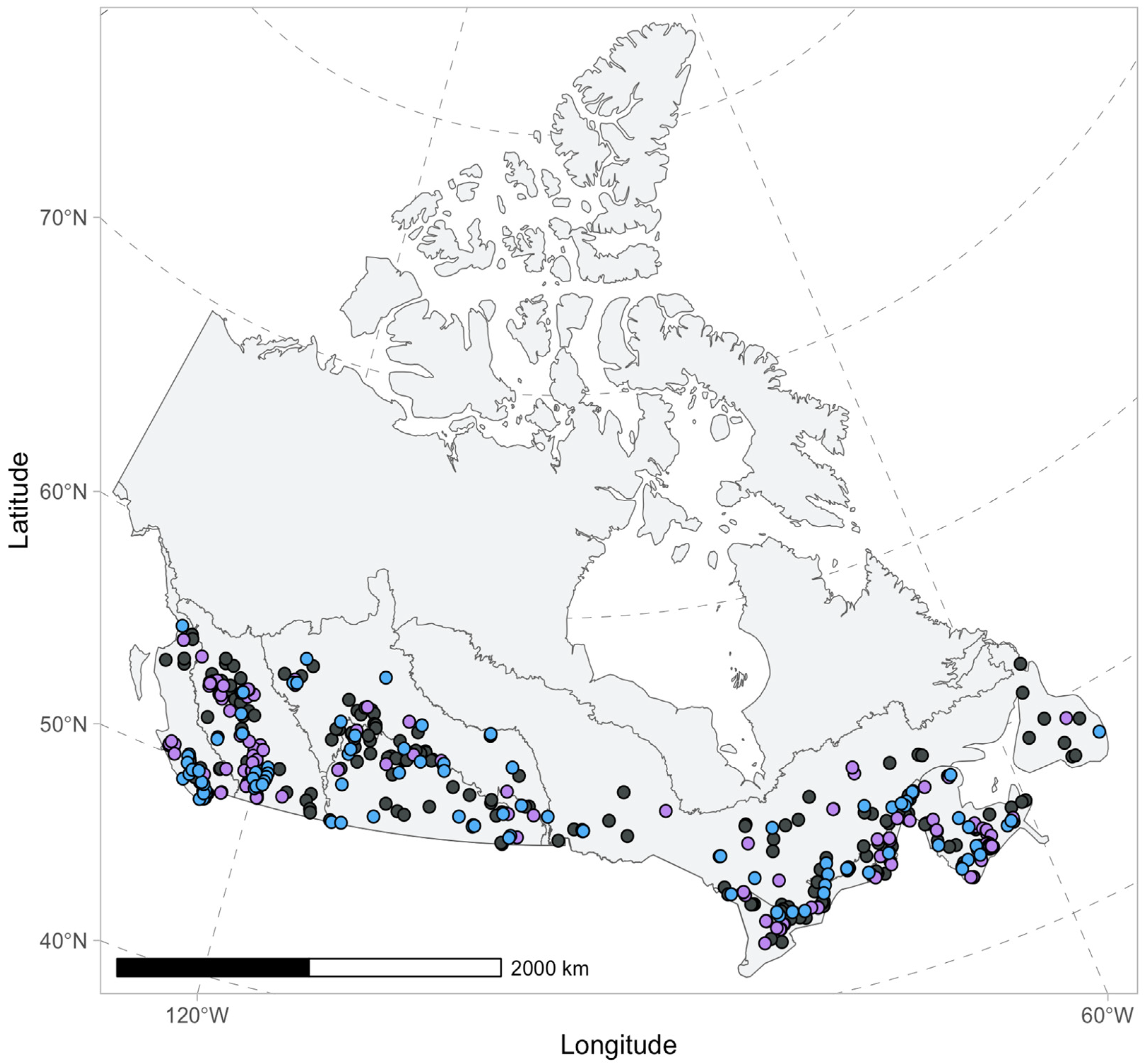
2.1. Study Site

Canada is a lake-rich country with a vast number of lakes distributed around its territory: it is estimated that there are over 900,000 lakes greater than 10 hectares that account for approximately 7% of the surface area of the country [20]. These lakes are distributed throughout the landscape, but not uniformly. Lake formation is influenced by geology and availability of water, and as such there is a higher density of lakes in northern and eastern Canada [20,48]. Many lakes, especially those located in northern Canada, are largely inaccessible and have never been sampled. As such, this study focused on lakes sampled in the southern portion of the country where in situ samples were available for calibration.

2.2. In Situ Data Collection

The data for this study was collected by the NSERC Canadian Lake Pulse Network, a research partnership between academia and government designed to provide Canada’s first national-scale assessment of lake health [47]. Sampled lakes were selected in a semi-random sampling design with ecozone, human impact index, and lake size as stratifying factors. Sampling occurred during the period of maximum summer lake stratification (late June to mid-September) to eliminate seasonal effects. During these sampling campaigns, the Lake Pulse teams measured approximately 100 water-quality parameters, including CDOM absorption spectra from 664 lakes. Although Lake Pulse field crews sampled lakes across all 10 Canadian provinces and 2 territories (Northwest Territories and Yukon), we only used data that coincided with the ecozones in the southern half of Canada (n = 592). This was firstly because few samples were taken in the far north of Canada, and secondly because surface reflectance imagery for Landsat 8 data is only reliable at latitudes below 65° [49].

Sampling procedures for field and laboratory analyses followed standard limnological practices [50]. For CDOM, a single sample per lake was collected from the epilimnion. Water for CDOM analysis was filtered through a 0.45 μm filter and stored in the dark at 4 °C in 60 mL Amber Boston Round Glass Bottles until the time of processing in the lab. Before lab analysis, samples were refiltered with 0.2 μm filters. CDOM was determined from absorbance measurements at 440 nm (a₄₄₀) using a Perkins-Elmer lambda 650 spectrophotometer using the dual-beam mode through 5 or 10 cm quartz cuvettes against a sample of deionised water. Absorbance was converted to Napierian absorption coefficients [51] using:

a₄₄₀ = 2.303 * Absa₄₄₀/l,

(1)

where a₄₄₀ is the absorption coefficient, 2.303 is the natural logarithm of 10, Absa₄₄₀ is absorbance, and l is the cell path length of the cuvette (m). Additionally, the a_CDOM spectrums were corrected for temperature differences between the deionized water and lake samples [52]. CDOM values are reported as a₄₄₀ (m⁻¹).

2.3. Image Collection and Processing

We used Google Earth Engine (GEE) [53] to obtain Landsat 8 Tier 1 Surface Reflectance images from the U.S. Geological Survey (USGS) [49]. These images have been atmospherically corrected using the Land Surface Reflectance Code (LaSRC) [25]. The LaSRC algorithm is optimized for land rather than aquatic systems, but the product is nonetheless successfully used for lake-monitoring applications for the estimation of CDOM [17,54,55].

We extracted mean surface reflectance values from a 50 m buffer around each sample location using images with cloud cover ≤30%. Specifically, we extracted data in bands B1–B5 (ultra-blue, blue, green, red, near-infrared). We filtered the image data for each of the extracted buffer zones using the bit quality assessment (BQA) band [56,57] in order to remove cloud and cloud shadow. The image data for each of the extracted buffer zones were also filtered so that only images with a BQA band value of 324, signaling cloud-free water, were included. The remaining data were then filtered to remove any null values that occurred due to cloud and cloud shadow masking.

Of the lakes sampled for CDOM between 2017 and 2019 by the NSERC Canadian Lake Pulse Network, we identified those that were at least 10 ha large with observations 20 m or greater from shore (when including the 50 m buffer). For 329 of the lakes, we identified clear summer imagery within 30 days of the sample date (between 20 June–20 September). Of the 329 lakes, we randomly identified 233 of these lake samples for model calibration, leaving 96 for model validation (Figure 1). Calibration and validation lakes were distributed throughout the southern half of Canada and had a similar range of CDOM(a₄₄₀). For the calibration dataset, CDOM(a₄₄₀) values ranged between 0.05 and 11.5 m⁻¹, whereas for the validation dataset, values ranged between 0.06 and 10.5 m⁻¹. An additional 128 lakes were sampled by Pulse that did not have imagery within 30 days of the sample date. They were retained for subsequent use as an illustration of how this approach can be extended to larger numbers of lakes than in other approaches using narrow time windows. These lakes had estimated average lake depths that ranged from 1–143 m and estimated size that ranged from 0.1–964 km² [20].

2.4. Coloured Dissolved Organic Matter Modelling

2.4.1. Predictor Selection

We began by testing multiple time windows using a unique image. We tested time windows of ±1, ±3, ±7, and ±30 days. For these narrower time windows, there were very few sample points available for algorithm development and testing (17, 50, and 101 lakes, respectively), which would not be applicable to a continental scale approach. Of the 592 NSERC Canadian Lake Pulse Network lakes, 329 (233 calibration, 96 validation) were sampled within a 30-day window of a clear image. We used these lakes as the basis to explore the effect of incorporating more imagery into the analysis, while leaving other factors fixed.

We used the random forest technique to select relevant variables using image data from ± 30 days of the in situ collection date (Thirty-day Window Nearest). We created random forests of potential explanatory band combinations using the VSURF package in R [58,59] and assessed the most significant combinations. We used the calibration dataset of measured CDOM(a₄₄₀) values as the dependent variable, and the surface reflectance values for Landsat 8 OLI bands B1–B5 and band ratio permutations from the Same Month Single Image temporal window as the independent variables (26 terms total). We used variables identified by the “prediction step” [58] and identified the pair of terms that produced the highest adjusted R² and lowest root mean squared error (RMSE) to develop the models. To ensure that there were no spatial boundaries that needed to be considered for the algorithm calibration process, we mapped and graphed residuals to identify any spatial clustering of extreme residual values.

2.4.2. Time Windows

For each lake in the calibration and validation datasets, there was a substantial number of images in the Google Earth Engine catalog that could potentially improve the explanatory power of imagery for estimating CDOM in Canadian lakes. For each lake in the calibration and validation datasets, we identified images that fit the following time constraints:

• Thirty-day Window Nearest: image reflectance for a single satellite image taken nearest in time within ±30 days of the in situ collection date, following Brezonik et al. [26], Olmanson et al. [17], and others (124 images, 1 observation per lake).
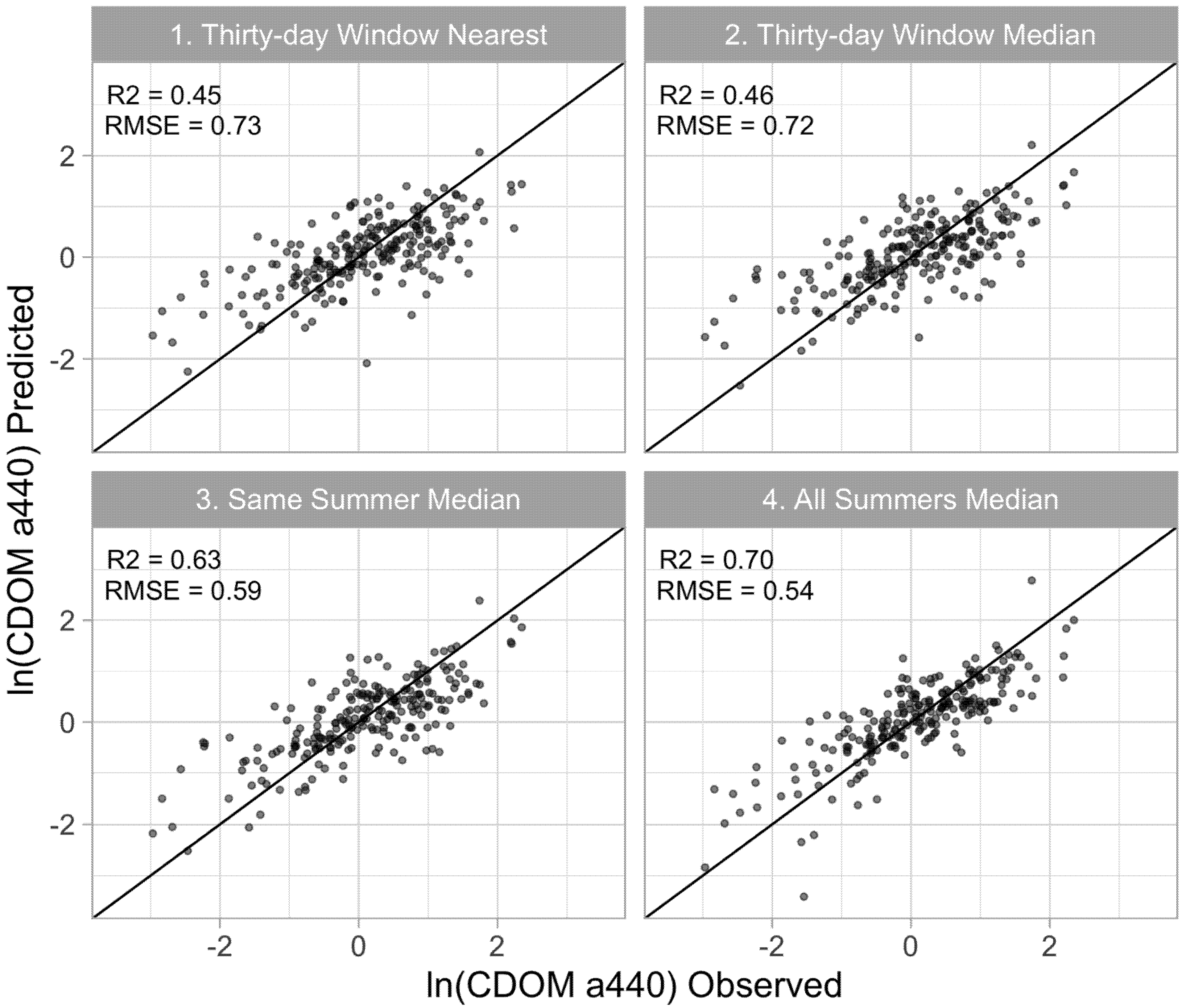
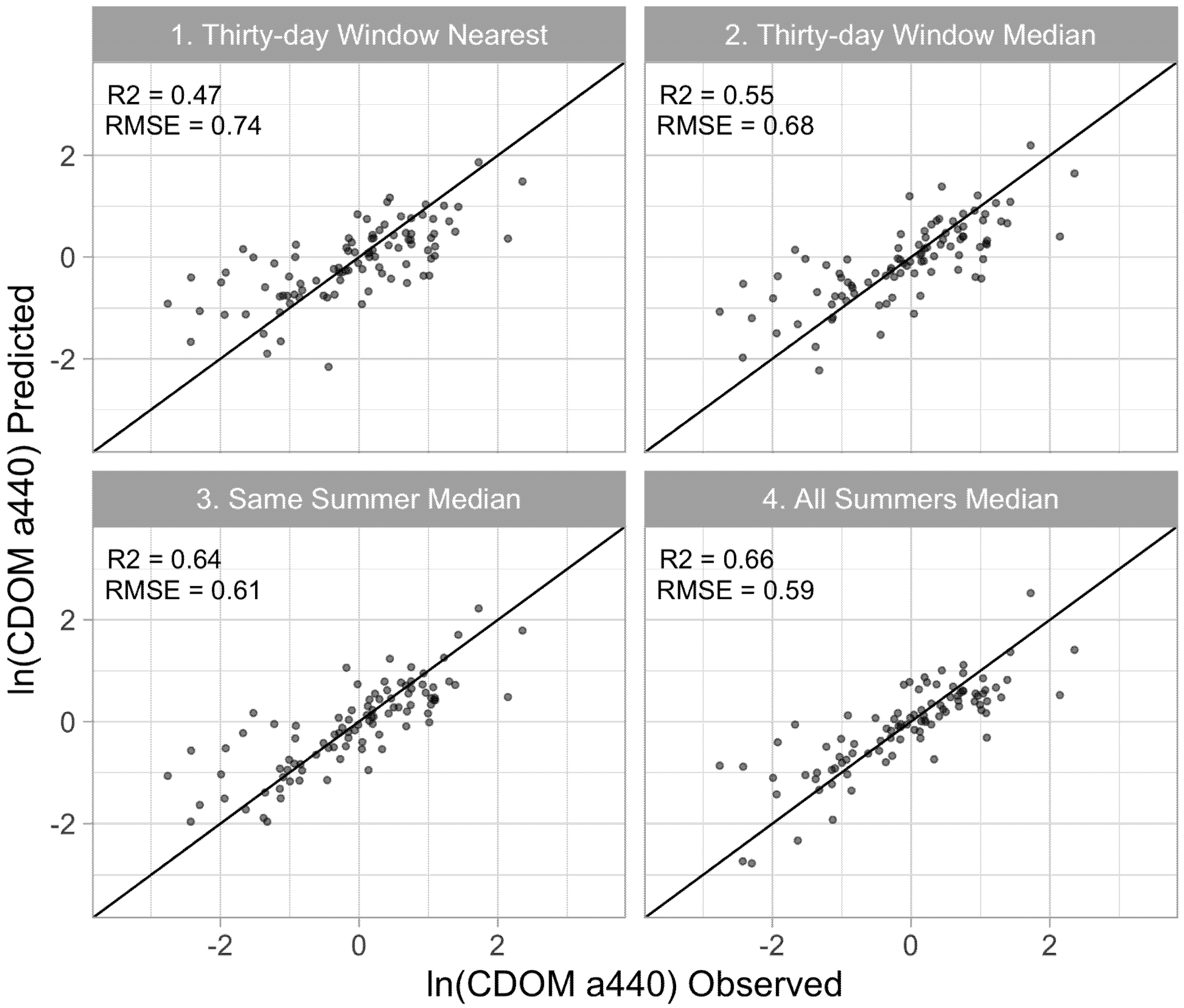
• Thirty-day Window Median: median image reflectance within ±30 days of the in situ sample date for each sample station (242 images, average 2.2 images per lake).
• Same Summer Median: median image reflectance within the same summer (20 June–20 September); the in situ sample was taken for each sample station (305 images, average 3.2 images per lake).
• All Summers Median: median image reflectance of all available summer images (20 June–20 September) throughout the Landsat record (2013–2019) for each sample station (2290 images, average 23.8 images per lake).

For both the calibration and validation datasets, we compared the model fit for the various time windows using model adjusted R², RMSE, which is the square root of the mean of squares of all errors [60]; mean absolute error (MAE), which is the mean of the absolute values of the individual prediction errors [61]; and statistical bias [62], which computes the average amount of error using the metrics package [62] in the R software [63].

$$\mathrm{MAE}=\frac{{{\displaystyle \sum }}_{i=1}^n\left|\mathrm{CDOM}\left(a440\right),sensor-\mathrm{CDOM}\left(a440\right), in situ\right|}{n}$$

(2)

where CDOM(a₄₄₀), sensor is using Landsat 8 SR data. MAE= 0 equals a perfect fit.

$$\mathrm{RMSE}=\sqrt{\frac{{{\displaystyle \sum }}_{i=1}^n {\left(\mathrm{CDOM}\left(a440\right),sensor-\mathrm{CDOM}\left(a440\right), in situ\right)}^2}{n}}$$

(3)

where CDOM(a₄₄₀), sensor is using Landsat 8 SR data. RMSE= 0 equals a perfect fit.

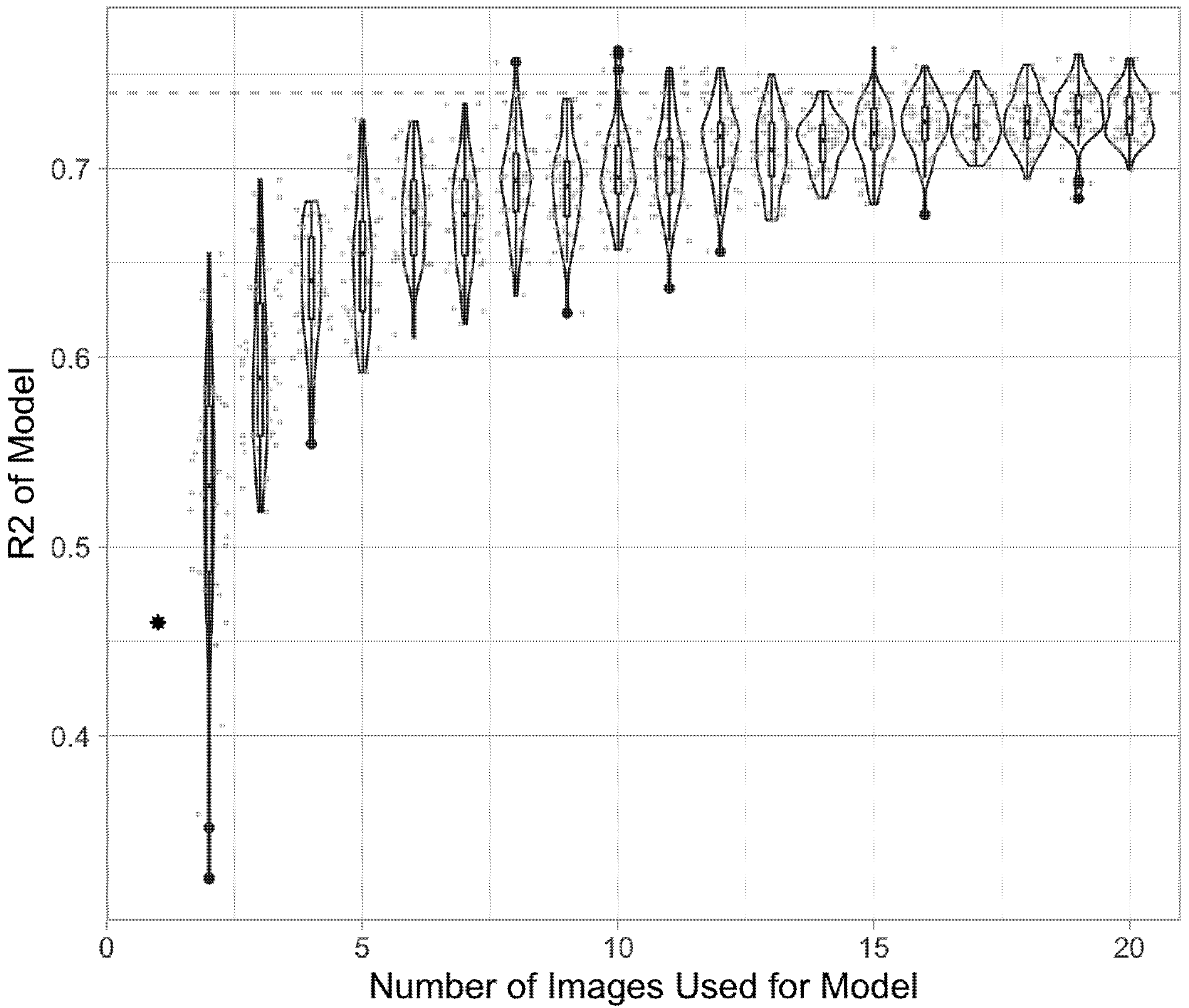
2.4.3. Effects of Adding Imagery

To understand the potential effect of increasing the amount of imagery considered when creating a regression relationship, we identified 118 (of 233) lakes from the calibration dataset that had 20 or more clear summer images over the 2013 to 2019 period. We iteratively selected images from this 20-image pool, without regard for the proximity of the images to the sample collection date and used them to create regressions using the same variables (B3/B4, B2) as those used for the “Thirty-day Window Nearest” progression. We then determined the asymptote of the distribution by using the Stats package [63] to implement the nls() function.

2.4.4. Extra Lakes Considered when the Time Window Was Expanded

We included lakes that would not have been considered in studies limited to only a single tight timeframe for image selection. These were 128 lakes for which there were no clear image matches within 30 days of in situ sampling and satellite overpass; CDOM(a₄₄₀) values ranged between 0.03 and 10.25 m⁻¹ (Figure 1). We assessed model performance for two time windows: (1) Same Summer Median, and (2) All Summers Median.

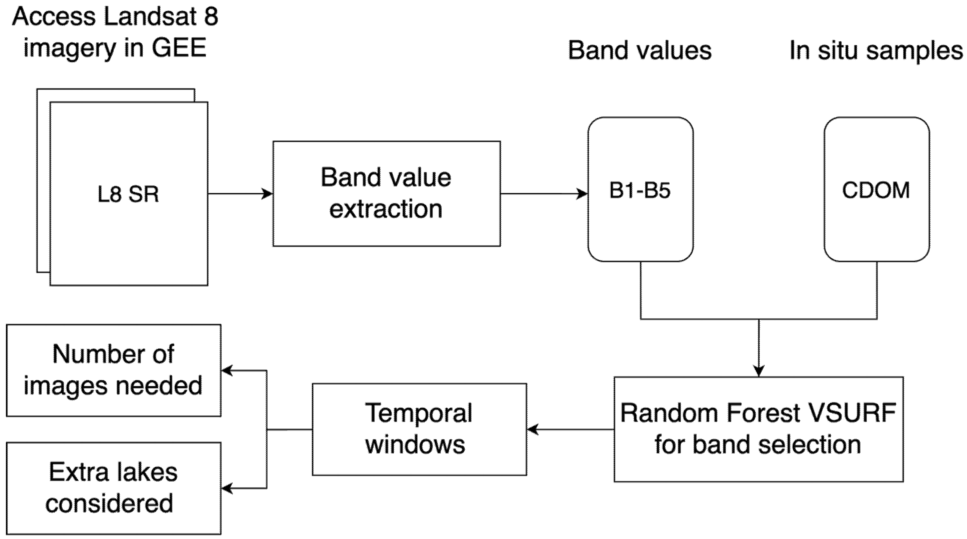
2.4.5. Overall Workflow

The overall workflow of the methods section can be seen in Figure 2. Landsat 8 surface reflectance imagery was accessed in GEE, and band values for B1–B5 were extracted. These band values for a single clear image within a 30-day window were used in conjunction with the in situ CDOM(a₄₄₀) samples for the random forest using VSURF for band selection. At this stage we examined how using various time windows using a median filter impacted the results. We then explored the potential effect of increasing the amount of imagery using the median filter. Finally, we looked at an extra set of lakes in order to see how the model performed in lakes that had neither been used for model calibration or validation.

3. Results

3.1. CDOM Model Results

Based on the results of the random forest using VSURF, we identified the best two-termed model as:

ln(CDOM(a₄₄₀)) = a − b(ln(B3/B4)) − c(ln(B2)

(4)

where ln(CDOM(a₄₄₀)) is the natural logarithm of the CDOM absorbance coefficient measured at 440 nm for a given sample location; coefficients a, b, and c were fit to the calibration data by regression analysis; and B3, B4, and B2 represent Landsat 8’s green, red, and blue bands, respectively. The first term (B3/B4) explained most of the variance observed, and was improved slightly by including the second term (B2) (Figure S1). Random Forest runs on data with other time windows produced similar variable choices.

3.2. Using More Than One Image for Model Development

Given the results of our assessment of spatial variability in regression coefficients, we created a global regression model with the “Thirty-day Window Nearest” time window (ln(CDOM(a₄₄₀)) = 3.65 − 2.91 * ln(B3/B4) − 0.41 * ln(B2), p-value < 2.2 * 10⁻¹⁶, adjusted R² = 0.47). Models built from very narrow time windows, which included only lakes with satellite overpass within one, three, or seven days, covered dramatically fewer lakes and offered no improvement in accuracy metrics from the 30-day window model made from a single image (Table S1). We mapped the standardised regression residuals to assess if there were any spatial patterns in statistically significant residual values (Figure 3). Most standardised regression residuals fell within 1.96 standard deviations of the mean for this study, with little apparent spatial pattern in how positive and negative they were throughout the country.

Because our spatial assessment indicated no clear geographical boundaries for algorithm coefficients, we proceeded using a global algorithm using all of the data to test three methods for estimating the satellite’s response for model calibration. Calibration regression models for the median filters for the four time window lengths are shown in

Table 1. Regression models estimating in situ CDOM(a₄₄₀) from Landsat 8 B3/B4 and B2 surface reflectance for different time windows. RMSE = root mean square error.

Time Window	Sample Size	Intercept	Coefficient (G/R)	Coefficient (B)	RMSE	MAE	Bias	Adj. R2	Valid-ation Adj. R2	Extra Lakes Adj R2
Thirty-day Window Nearest	233	3.96	−2.91	−0.46	0.73	0.55	0.31	0.45	0.47	n/a
Thirty-day Window Median	233	4.04	−3.1	−0.46	0.72	0.54	0.29	0.46	0.55	n/a
Median of Same Summer	233	5	−3.89	−0.58	0.59	0.49	0.235	0.63	0.64	0.49
Median of All Summers	233	4.41	−4.14	−0.46	0.54	0.43	0.19	0.7	0.66	0.57

. Model fit significantly improved when increasing data input by taking median image values from one month (adjusted R² = 0.46) to same year (adjusted R² = 0.63), and then again to input from all years (adjusted R² = 0.70), with the predictions tightening around the 1:1 line (Figure 4). RMSE also decreased significantly with increasing time window sizes for each of the median filters. Model coefficients (slope) also decreased with larger time window size when taking median image values, with low CDOM(a₄₄₀) values tending to be overestimated and larger CDOM(a₄₄₀) values underestimated in models using smaller time windows (Figure 4).

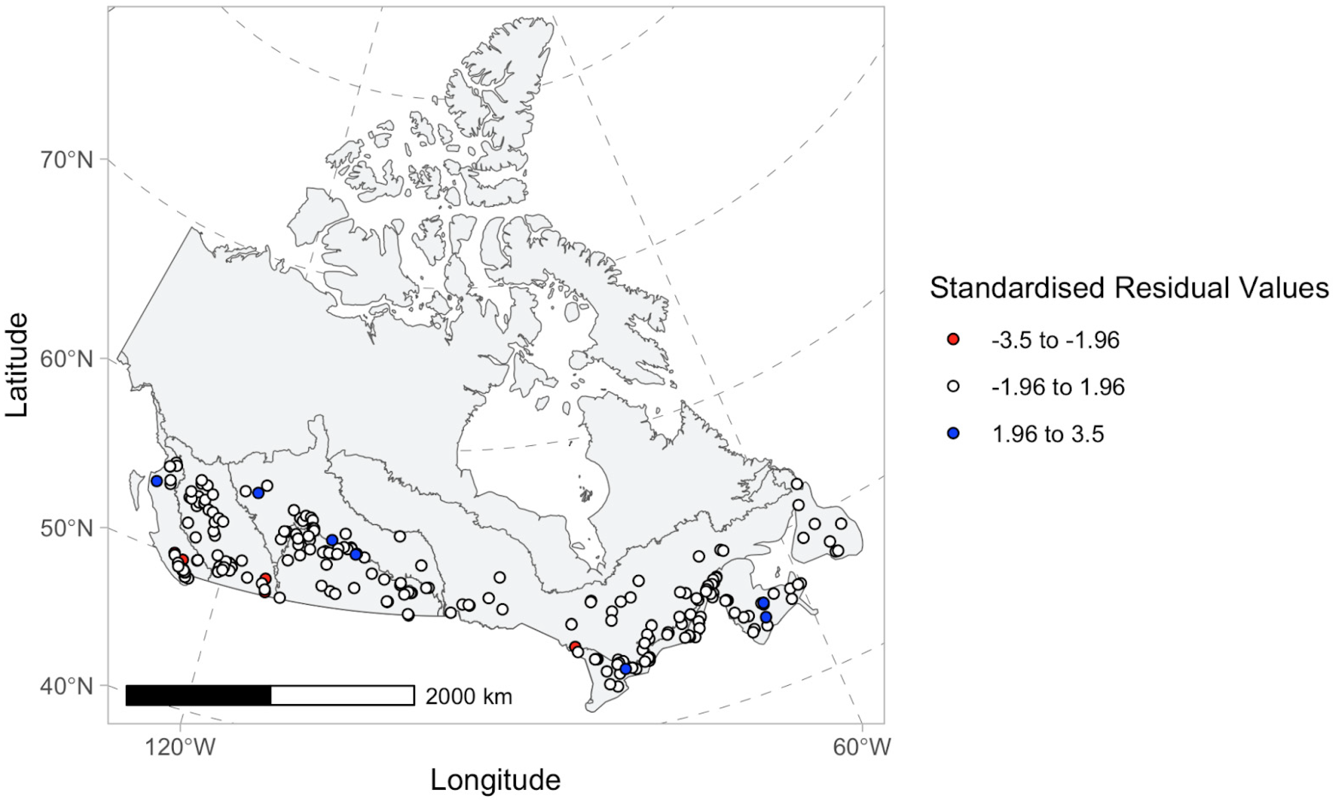
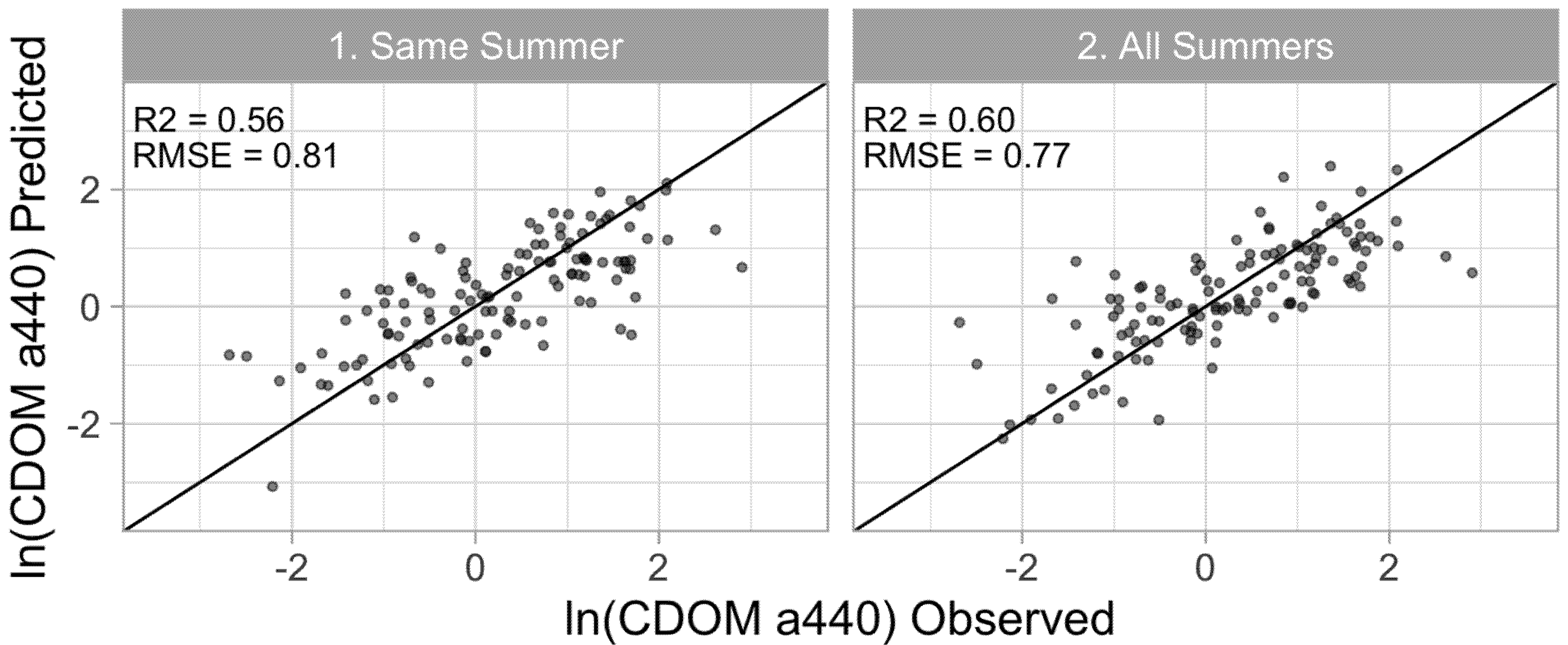
3.3. Model Validation

As in the calibration results, the quality of the CDOM(a₄₄₀) prediction in the validation lake set grew quickly with more imagery (Figure 5). For each time window, the fit in the validation set was quite similar to that in the calibration set—e.g., adjusted R² = 0.70 for the all-images model in the calibration set versus adjusted R² = 0.66 in the validation set. The results showed (Figure 5) that the models effectively predicted values of CDOM > ln(0) (CDOM > 1) for the various time windows, while low values of CDOM(a₄₄₀) were consistently overestimated. This overestimation was somewhat reduced in models using data from all years.

3.4. Effects of Adding Imagery

Increased amounts of imagery improved the ability to predict field-gathered CDOM(a₄₄₀) values (Figure 6). In 118 of the 233 calibration lakes across Canada for which at least 20 clear images were available, better and more consistent regression models were formed as more imagery was added. Considering the same set of 118 lakes, selecting more images from any summer date in the Landsat 8 record systematically improved the regression model between imagery and CDOM (Figure 6). Using a carefully curated single image nearest in time to the sample date, the model had adjusted R² = 0.45; that model could be considerably improved in the imagery-rich lake subset by selecting any three summer images and taking the median ratio, raising the expected adjusted R² to about 0.57. Notably, models formed by taking any three randomly selected images were all better than the model with one carefully curated image. The effect of including more imagery leveled off around 12 images, with an expected upper bound asymptote near an adjusted R² of 0.74 (Figure 6).

3.5. Extra Lakes Considered When the Time Window Was Expanded

In such models that do not require tight timing of field and satellite data, substantially more lakes can be included in a research study. In this dataset, 128 lakes had no clear image within a 30-day window, which would exclude them from model calibration/validation in other approaches. Using the median of band ratios from the rest of the Landsat 8 satellite record, these 128 lakes broadly fit the pattern of the calibration and validation lakes, clustering around the 1:1 line—though with somewhat more scatter in the set of extra lakes (Figure 7). The scatter seemed to be greater for low values of CDOM(a₄₄₀) in particular. However, by including these lakes, we were able to increase the number of lakes under consideration from 329 to 457, equating to a nearly 40% increase. This demonstrated that future studies could include lakes without matches within a 30-day window for model calibration and validation.

4. Discussion

This study explored the creation of models for predicting field-sampled CDOM in a fixed set of lakes. Gathering and incorporating information from more Landsat 8 images improved our ability to estimate CDOM levels in hundreds of lakes. What was found was that, for a large number of varied lakes across Canada, the median of multiple images was a powerful and robust noise-dampening approach to model development. We were surprised at the strength of adding more images for a large number of lakes across a large portion of southern Canada. In effect, one could select any four summer images and be virtually guaranteed of a model that was superior to one created from a single, curated image near the field sample date. The use of an ensemble of images, even an ensemble of modest size, greatly aided CDOM estimation across a very large area.

Given the time, effort, and expense of gathering field data for CDOM model fits, and the relatively small proportion of Canada’s nearly 1 million lakes larger than 10 ha [20] that have been sampled, field data is a rare resource, and its use should be maximized. In addition to improving the fit of CDOM models, the median method expands the number of lakes that can be considered. Without the constraint of matching cloud-free imagery to a costly field campaign, we were able to considerably expand the scope of analysis. An effective fit in a large number of lakes at a continental scale is especially useful given lingering challenges to transferring or extrapolating models made from a small number of lakes [30,55,64]. In that light, the predictive power of the preferred model in this study can be considered good (adjusted R² = 0.70, RMSE = 0.54 for the “All Summers Median” model). This is especially the case for CDOM, which is a challenging water property to estimate at broad scales in inland waters [26,65,66].

We found no spatial pattern in residuals of the model fit, indicating that there were no spatial boundaries that needed to be respected for the algorithm calibration process. This was unexpected, given the expanse of the study area and the wide range of lake types encompassed in the study. In previous studies, algorithms are usually locally calibrated either for individual lakes or regions of similar lakes [23,31,43,67] to consider the variability of lake types encompassed in a study. Therefore, algorithm calibration has mainly been tested across a more limited range of lake optical types. However, Deutsch et al. [35] similarly found that a single global algorithm could be used to estimate Secchi disk depth for a large dataset of lakes spread across southern Canada. However, note that both the calibration and validation datasets lacked high CDOM lakes (>11.5 and 10.5 m⁻¹, respectively). Therefore, models developed in this study are applicable only to lakes with low to moderate CDOM levels. Additionally, the model proposed tended to overpredict CDOM(a₄₄₀) values in lakes with CDOM(a₄₄₀) < 1 m⁻¹, but this trend was partially mitigated using the “All Summers Median” time window. For future research concerned with pinpointing CDOM concentration in low-CDOM lakes, additional band ratios or other information could be considered.

In this study, we found that taking median satellite image values using increasingly wide time windows consistently resulted in improved algorithm fit (Figure 3). One likely reason we saw this improvement is that repeat satellite data over a given location is inherently variable due to atmospheric influences [68]. By adding more data to the analysis and assessing median band and band ratio data, it is possible that we removed atmospheric artifacts that were not already filtered out through atmospheric correction and data cleaning steps. Therefore, it is possible that taking median satellite image values over wider time windows helped us better observe the true Landsat 8 B3/B4 and B2 surface reflectance over a given water pixel.

We expect that the effectiveness of using the median will be strongest when image-to-image variability is greater than in-lake and among-lake CDOM variability. Each of the remote lakes in this study was visited only once, with a sample taken at a single point in each lake, making it difficult to quantify in-lake CDOM temporal variability. Because the method averages image values from a potentially long period of time, it is not intended to track changes in CDOM over short time scales. That said, many studies have found CDOM to be relatively stable when examining within-season timescales [26,28,69,70]. Other works have found that, at least in some lakes, CDOM can fluctuate over short time windows [17,71]. At decadal time scales, CDOM and related DOC levels have been found to be increasing in freshwaters across boreal and temperate regions in North America and Europe [1,2,72], which has been linked to the decrease of acid rain as a result of the emissions regulations that have been put in place in Europe and North America [2,73]. However, for the specific set of lakes in this study that were sampled from June until September, this variability was apparently not sufficient to limit the effectiveness of median satellite image values over time windows as large as seven years (2013–2019). It is possible that this method would not be applicable during other seasons of the year, when water conditions within lakes may change more rapidly [26].

Despite the apparent dampening effect of the median of a group of images, there were still sources of error and uncertainty that could limit performance in results seen here. First, we did not actively seek out region-specific models at this stage; it is possible that regional models could have improved the fit, at least for some lakes. Second, there may well be other sources of colour than CDOM, particularly in more eutrophic conditions. This might account for some of the variability in higher-CDOM conditions, and might be separately treated in future work. Third, for any given lake, there are additional sources of variability not explored here: CDOM concentration changes throughout a summer and across years, and may vary substantially in different parts of a given lake. Finally, though we tried to create a model that could be used to make broad estimates in a wide range of Canadian lakes, it is worth noting explicitly that only a small fraction of Canada’s vast lake resource was sampled; the model may not be applicable to all lakes in southern Canada.

Future directions for this work could explore how using colour space transformations and optical water properties might improve CDOM(a₄₄₀) estimates. Transformations to hue–saturation–intensity (HSI) is a simple colour transformation that can be used to develop colour-based image-processing techniques. Niroumand-Jadidi et al. [74] found that colour space transformations showed benefits for estimating water-quality parameters including CDOM. Another possible direction to improve water-quality estimates would be to develop algorithms specifically based on the optical properties of a given waterbody. Various hierarchical, partitional, and hybrid clustering techniques have been used to successfully classify remote sensing reflectance (Rrs) into groups [75,76,77]. Since the NSERC Canadian Lake Pulse Network collected data on various optical water properties as well as in situ reflectance data, classification based on optical types could be explored. Specifically, total suspended sediments (TSS); algal biomass, measured as chlorophyll a (chl-a); and coloured dissolved organic matter (CDOM) data were collected.

Future work could also add other satellite sensors such as Sentinel-2 and Landsat 9, scheduled for launch in autumn 2021. Water-quality parameters have already been successfully estimated using workflows that harmonised Landsat 8 OLI and Sentinel-2 MSI imagery products in Google Earth Engine [17,42], suggesting possible joint Landsat/Sentinel models. By employing harmonised imagery from multiple sensors, revisit time would be reduced, which could considerably increase the chances of obtaining a high number of clear summer images.

5. Conclusions

While creating high-quality models of coloured dissolved organic matter (CDOM) across a lake-rich region, this study demonstrated the benefit, at least in these lakes, of adding additional imagery to sharpen the signal derived from remote sensing. Additionally, this study effectively expanded the number of lakes that were available for consideration: using a larger set of freely available imagery, we were able to make plausible estimates of CDOM in 40% more lakes than if we had used narrower time windows. As we consider projecting results across very large areas, such as continental scales as seen in the study, the ability to consolidate information from a variety of dates provides an opportunity that is lacking if we were to only use data from a single narrowly timed image.

References

1. Creed, I.F.; Bergström, A.-K.; Trick, C.G.; Grimm, N.B.; Hessen, D.O.; Karlsson, J.; Kidd, K.A.; Kritzberg, E.; McKnight, D.M.; Freeman, E.C.; et al. Global Change-Driven Effects on Dissolved Organic Matter Composition: Implications for Food Webs of Northern Lakes. Glob. Chang. Biol. 2018, 24, 3692–3714. [Google Scholar] [CrossRef]
2. Solomon, C.T.; Jones, S.E.; Weidel, B.C.; Buffam, I.; Fork, M.L.; Karlsson, J.; Larsen, S.; Lennon, J.T.; Read, J.S.; Sadro, S.; et al. Ecosystem Consequences of Changing Inputs of Terrestrial Dissolved Organic Matter to Lakes: Current Knowledge and Future Challenges. Ecosystems 2015, 18, 376–389. [Google Scholar] [CrossRef]
3. Hudson, N.; Baker, A.; Reynolds, D. Fluorescence Analysis of Dissolved Organic Matter in Natural, Waste and Polluted Waters—A Review. River Res. Appl. 2007, 23, 631–649. [Google Scholar] [CrossRef]
4. Brezonik, P.; Arnold, W.A. Water Chemistry: An Introduction to the Chemistry of Natural and Engineered Aquatic Systems; Oxford University Press: New York, NY, USA, 2011; ISBN 978-0-19-973072-8. [Google Scholar]
5. Chen, Y.; Arnold, W.A.; Griffin, C.G.; Olmanson, L.G.; Brezonik, P.L.; Hozalski, R.M. Assessment of the Chlorine Demand and Disinfection Byproduct Formation Potential of Surface Waters via Satellite Remote Sensing. Water Res. 2019, 165, 115001. [Google Scholar] [CrossRef]
6. Gaiser, E.E.; Deyrup, N.D.; Bachmann, R.W.; Battoe, L.E.; Swain, H.M. Effects of Climate Variability on Transparency and Thermal Structure in Subtropical, Monomictic Lake Annie, Florida. Fundam. Appl. Limnol. 2009, 175, 217–230. [Google Scholar] [CrossRef]
7. Heijerick, D.G.; Janssen, C.R.; Coen, W.M.D. The Combined Effects of Hardness, PH, and Dissolved Organic Carbon on the Chronic Toxicity of Zn to D. Magna: Development of a Surface Response Model. Arch. Environ. Contam. Toxicol. 2003, 44, 210–217. [Google Scholar] [CrossRef] [PubMed]
8. Houser, J.N. Water Color Affects the Stratification, Surface Temperature, Heat Content, and Mean Epilimnetic Irradiance of Small Lakes. Can. J. Fish. Aquat. Sci. 2006, 63, 2447–2455. [Google Scholar] [CrossRef]
9. Pilla, R.M.; Williamson, C.E.; Zhang, J.; Smyth, R.L.; Lenters, J.D.; Brentrup, J.A.; Knoll, L.B.; Fisher, T.J. Browning-Related Decreases in Water Transparency Lead to Long-Term Increases in Surface Water Temperature and Thermal Stratification in Two Small Lakes. J. Geophys. Res. Biogeosci. 2018, 123, 1651–1665. [Google Scholar] [CrossRef]
10. Thrane, J.-E.; Hessen, D.O.; Andersen, T. The Absorption of Light in Lakes: Negative Impact of Dissolved Organic Carbon on Primary Productivity. Ecosystems 2014, 17, 1040–1052. [Google Scholar] [CrossRef] [Green Version]
11. Lapierre, J.-F.; Guillemette, F.; Berggren, M.; del Giorgio, P.A. Increases in Terrestrially Derived Carbon Stimulate Organic Carbon Processing and CO2 Emissions in Boreal Aquatic Ecosystems. Nat. Commun. 2013, 4, 2972. [Google Scholar] [CrossRef]
12. Song, G.; Li, Y.; Hu, S.; Li, G.; Zhao, R.; Sun, X.; Xie, H. Photobleaching of Chromophoric Dissolved Organic Matter (CDOM) in the Yangtze River Estuary: Kinetics and Effects of Temperature, PH, and Salinity. Environ. Sci. Process. Impacts 2017, 19, 861–873. [Google Scholar] [CrossRef] [PubMed]
13. Blewett, T.A.; Dow, E.M.; Wood, C.M.; McGeer, J.C.; Smith, D.S. The Role of Dissolved Organic Carbon Concentration and Composition on Nickel Toxicity to Early Life-Stages of the Blue Mussel Mytilus Edulis and Purple Sea Urchin Strongylocentrotus Purpuratus. Ecotoxicol. Environ. Saf. 2018, 160, 162–170. [Google Scholar] [CrossRef]
14. Schwartz, M.L.; Curtis, P.J.; Playle, R.C. Influence of Natural Organic Matter Source on Acute Copper, Lead, and Cadmium Toxicity to Rainbow Trout (Oncorhynchus Mykiss). Environ. Toxicol. Chem. 2004, 23, 2889. [Google Scholar] [CrossRef] [PubMed]
15. Grünwald, A.; Šťastný, B.; Slavíčková, K.; Slavíček, M. Formation of Haloforms during Chlorination of Natural Waters. Acta Polytech. 2002, 42. [Google Scholar] [CrossRef]
16. Minear, R.A.; Amy, G.L. Disinfection By-Products in Water Treatment: The Chemistrg of Their Formation and Control; CRC Press: Boca Raton, FL, USA, 1996; ISBN 978-1-315-14135-0. [Google Scholar]
17. Olmanson, L.G.; Page, B.P.; Finlay, J.C.; Brezonik, P.L.; Bauer, M.E.; Griffin, C.G.; Hozalski, R.M. Regional Measurements and Spatial/Temporal Analysis of CDOM in 10,000+ Optically Variable Minnesota Lakes Using Landsat 8 Imagery. Sci. Total Environ. 2020, 724, 138141. [Google Scholar] [CrossRef] [PubMed]
18. Ross, M.R.V.; Topp, S.N.; Appling, A.P.; Yang, X.; Kuhn, C.; Butman, D.; Simard, M.; Pavelsky, T.M. AquaSat: A Data Set to Enable Remote Sensing of Water Quality for Inland Waters. Water Resour. Res. 2019, 55, 10012–10025. [Google Scholar] [CrossRef]
19. Stanley, E.H.; Powers, S.M.; Lottig, N.R.; Buffam, I.; Crawford, J.T. Contemporary Changes in Dissolved Organic Carbon (DOC) in Human-Dominated Rivers: Is There a Role for DOC Management? Freshw. Biol. 2012, 57, 26–42. [Google Scholar] [CrossRef]
20. Messager, M.L.; Lehner, B.; Grill, G.; Nedeva, I.; Schmitt, O. Estimating the Volume and Age of Water Stored in Global Lakes Using a Geo-Statistical Approach. Nat. Commun. 2016, 7, 13603. [Google Scholar] [CrossRef]
21. Mannino, A.; Russ, M.E.; Hooker, S.B. Algorithm Development and Validation for Satellite-Derived Distributions of DOC and CDOM in the U.S. Middle Atlantic Bight. J. Geophys. Res. 2008, 113, C07051. [Google Scholar] [CrossRef]
22. Klein, I.; Gessner, U.; Dietz, A.J.; Kuenzer, C. Global WaterPack—A 250 m Resolution Dataset Revealing the Daily Dynamics of Global Inland Water Bodies. Remote Sens. Environ. 2017, 198, 345–362. [Google Scholar] [CrossRef]
23. Kutser, T.; Pierson, D.C.; Kallio, K.Y.; Reinart, A.; Sobek, S. Mapping Lake CDOM by Satellite Remote Sensing. Remote Sens. Environ. 2005, 94, 535–540. [Google Scholar] [CrossRef]
24. Mishra, D.R.; Ogashawara, I.; Gitelson, A.A. (Eds.) Bio-Optical Modelling and Remote Sensing of Inland Waters; Elsevier: Amsterdam, The Netherlands, 2017; ISBN 978-0-12-804644-9. [Google Scholar]
25. Vermote, E.; Justice, C.; Claverie, M.; Franch, B. Preliminary Analysis of the Performance of the Landsat 8/OLI Land Surface Reflectance Product. Remote Sens. Environ. 2016, 185, 46–56. [Google Scholar] [CrossRef] [PubMed]
26. Brezonik, P.; Olmanson, L.G.; Finlay, J.C.; Bauer, M.E. Factors Affecting the Measurement of CDOM by Remote Sensing of Optically Complex Inland Waters. Remote Sens. Environ. 2015, 157, 199–215. [Google Scholar] [CrossRef]
27. Chen, J.; Zhu, W.-N.; Tian, Y.Q.; Yu, Q. Estimation of Colored Dissolved Organic Matter From Landsat-8 Imagery for Complex Inland Water: Case Study of Lake Huron. IEEE Trans. Geosci. Remote Sens. 2017, 55, 2201–2212. [Google Scholar] [CrossRef]
28. Kutser, T.; Casal Pascual, G.; Barbosa, C.; Paavel, B.; Ferreira, R.; Carvalho, L.; Toming, K. Mapping Inland Water Carbon Content with Landsat 8 Data. Int. J. Remote Sens. 2016, 37, 2950–2961. [Google Scholar] [CrossRef]
29. Olmanson, L.G.; Brezonik, P.L.; Finlay, J.C.; Bauer, M.E. Comparison of Landsat 8 and Landsat 7 for Regional Measurements of CDOM and Water Clarity in Lakes. Remote Sens. Environ. 2016, 185, 119–128. [Google Scholar] [CrossRef]
30. Tyler, A.N.; Hunter, P.D.; Spyrakos, E.; Groom, S.; Constantinescu, A.M.; Kitchen, J. Developments in Earth Observation for the Assessment and Monitoring of Inland, Transitional, Coastal and Shelf-Sea Waters. Sci. Total Environ. 2016, 572, 1307–1321. [Google Scholar] [CrossRef] [Green Version]
31. Bonansea, M.; Rodriguez, M.C.; Pinotti, L.; Ferrero, S. Using Multi-Temporal Landsat Imagery and Linear Mixed Models for Assessing Water Quality Parameters in Río Tercero Reservoir (Argentina). Remote Sens. Environ. 2015, 158, 28–41. [Google Scholar] [CrossRef]
32. Brezonik, P.; Menken, K.D.; Bauer, M. Landsat-Based Remote Sensing of Lake Water Quality Characteristics, Including Chlorophyll and Colored Dissolved Organic Matter (CDOM). Lake Reserv. Manag. 2005, 21, 373–382. [Google Scholar] [CrossRef]
33. Cardille, J.A.; Leguet, J.-B.; del Giorgio, P. Remote Sensing of Lake CDOM Using Noncontemporaneous Field Data. Can. J. Remote Sens. 2013, 39, 118–126. [Google Scholar] [CrossRef]
34. Dekker, A.G.; Vos, R.J.; Peters, S.W.M. Analytical Algorithms for Lake Water TSM Estimation for Retrospective Analyses of TM and SPOT Sensor Data. Int. J. Remote Sens. 2002, 23, 15–35. [Google Scholar] [CrossRef]
35. Deutsch, E.S.; Cardille, J.A.; Koll-Egyed, T.; Fortin, M.-J. Landsat 8 Lake Water Clarity Empirical Algorithms: Large-Scale Calibration and Validation Using Government and Citizen Science Data from across Canada. Remote Sens. 2021, 13, 1257. [Google Scholar] [CrossRef]
36. Griffin, C.G.; McClelland, J.W.; Frey, K.E.; Fiske, G.; Holmes, R.M. Quantifying CDOM and DOC in Major Arctic Rivers during Ice-Free Conditions Using Landsat TM and ETM+ Data. Remote Sens. Environ. 2018, 209, 395–409. [Google Scholar] [CrossRef]
37. Kallio, K.; Attila, J.; Härmä, P.; Koponen, S.; Pulliainen, J.; Hyytiäinen, U.-M.; Pyhälahti, T. Landsat ETM+ Images in the Estimation of Seasonal Lake Water Quality in Boreal River Basins. Environ. Manag. 2008, 42, 511–522. [Google Scholar] [CrossRef] [PubMed]
38. Kuhn, C.; de Matos Valerio, A.; Ward, N.; Loken, L.; Sawakuchi, H.O.; Kampel, M.; Richey, J.; Stadler, P.; Crawford, J.; Striegl, R.; et al. Performance of Landsat-8 and Sentinel-2 Surface Reflectance Products for River Remote Sensing Retrievals of Chlorophyll-a and Turbidity. Remote Sens. Environ. 2019, 224, 104–118. [Google Scholar] [CrossRef] [Green Version]
39. Li, J.; Yu, Q.; Tian, Y.Q.; Becker, B.L.; Siqueira, P.; Torbick, N. Spatio-Temporal Variations of CDOM in Shallow Inland Waters from a Semi-Analytical Inversion of Landsat-8. Remote Sens. Environ. 2018, 218, 189–200. [Google Scholar] [CrossRef]
40. Lin, S.; Novitski, L.N.; Qi, J.; Stevenson, R.J. Landsat TM/ETM+ and Machine-Learning Algorithms for Limnological Studies and Algal Bloom Management of Inland Lakes. J. Appl. Remote Sens. 2018, 12, 026003. [Google Scholar] [CrossRef]
41. McCullough, I.M.; Loftin, C.S.; Sader, S.A. Combining Lake and Watershed Characteristics with Landsat TM Data for Remote Estimation of Regional Lake Clarity. Remote Sens. Environ. 2012, 123, 109–115. [Google Scholar] [CrossRef]
42. Page, B.P.; Olmanson, L.G.; Mishra, D.R. A Harmonized Image Processing Workflow Using Sentinel-2/MSI and Landsat-8/OLI for Mapping Water Clarity in Optically Variable Lake Systems. Remote Sens. Environ. 2019, 231, 111284. [Google Scholar] [CrossRef]
43. Matthews, M.W. A Current Review of Empirical Procedures of Remote Sensing in Inland and Near-Coastal Transitional Waters. Int. J. Remote Sens. 2011, 32, 6855–6899. [Google Scholar] [CrossRef]
44. Chen, T.; Ma, K.-K.; Chen, L.-H. Tri-State Median Filter for Image Denoising. IEEE Trans. Image Process. 1999, 8, 1834–1838. [Google Scholar] [CrossRef] [Green Version]
45. Gupta, G. Algorithm for Image Processing Using Improved Median Filter and Comparison of Mean, Median and Improved Median Filter. Int. J. Soft Comput. Eng. 2011, 1, 304–311. [Google Scholar]
46. Axelsson, A.; Lindberg, E.; Reese, H.; Olsson, H. Tree Species Classification Using Sentinel-2 Imagery and Bayesian Inference. Int. J. Appl. Earth Obs. Geoinform. 2021, 100, 102318. [Google Scholar] [CrossRef]
47. Huot, Y.; Brown, C.A.; Potvin, G.; Antoniades, D.; Baulch, H.M.; Beisner, B.E.; Bélanger, S.; Brazeau, S.; Cabana, H.; Cardille, J.A.; et al. The NSERC Canadian Lake Pulse Network: A National Assessment of Lake Health Providing Science for Water Management in a Changing Climate. Sci. Total Environ. 2019, 695, 133668. [Google Scholar] [CrossRef]
48. American Fisheries Society. Hubert, W.A., Quist, M.C., Eds.; Inland Fisheries Management in North America, 3rd ed.; American Fisheries Society: Bethesda, MD, USA, 2010; ISBN 978-1-934874-16-5. [Google Scholar]
49. U.S. Geological Survey. Landsat 8 (L8) Data Users Handbook; Earth Resources Observation and Science (EROS) Center: Sioux Falls, SD, USA, 2019.
50. Mobley, C.; Boss, E.; Roesler, C. Ocean Optics Web Book. 2020. Available online: http://www.oceanopticsbook.info (accessed on 1 September 2021).
51. Kirk, J.T.O. Light and Photosynthesis in Aquatic Ecosystems, 3rd ed.; Cambridge University Press: Cambridge, UK, 2010; ISBN 978-1-139-16821-2. [Google Scholar]
52. Langford, V.S.; McKinley, A.J.; Quickenden, T.I. Temperature Dependence of the Visible-Near-Infrared Absorption Spectrum of Liquid Water. J. Phys. Chem. A 2001, 105, 8916–8921. [Google Scholar] [CrossRef]
53. Gorelick, N.; Hancher, M.; Dixon, M.; Ilyushchenko, S.; Thau, D.; Moore, R. Google Earth Engine: Planetary-Scale Geospatial Analysis for Everyone. Remote Sens. Environ. 2017, 202, 18–27. [Google Scholar] [CrossRef]
54. Slonecker, E.T.; Jones, D.K.; Pellerin, B.A. The New Landsat 8 Potential for Remote Sensing of Colored Dissolved Organic Matter (CDOM). Mar. Pollut. Bull. 2016, 107, 518–527. [Google Scholar] [CrossRef]
55. Zhu, W.; Yu, Q.; Tian, Y.Q.; Becker, B.L.; Zheng, T.; Carrick, H.J. An Assessment of Remote Sensing Algorithms for Colored Dissolved Organic Matter in Complex Freshwater Environments. Remote Sens. Environ. 2014, 140, 766–778. [Google Scholar] [CrossRef]
56. Foga, S.; Scaramuzza, P.L.; Guo, S.; Zhu, Z.; Dilley, R.D.; Beckmann, T.; Schmidt, G.L.; Dwyer, J.L.; Joseph Hughes, M.; Laue, B. Cloud Detection Algorithm Comparison and Validation for Operational Landsat Data Products. Remote Sens. Environ. 2017, 194, 379–390. [Google Scholar] [CrossRef] [Green Version]
57. Zhu, Z.; Wang, S.; Woodcock, C.E. Improvement and Expansion of the Fmask Algorithm: Cloud, Cloud Shadow, and Snow Detection for Landsats 4–7, 8, and Sentinel 2 Images. Remote Sens. Environ. 2015, 159, 269–277. [Google Scholar] [CrossRef]
58. Genuer, R.; Poggi, J.-M.; Tuleau-Malot, C. Variable Selection Using Random Forests. Pattern Recognit. Lett. 2010. [Google Scholar] [CrossRef] [Green Version]
59. Liaw, A.; Wiener, M. Classification and regression by randomForest. R News 2002, 2, 18–22. [Google Scholar]
60. Neill, S.P.; Hashemi, M.R. Ocean Modelling for Resource Characterization. In Fundamentals of Ocean Renewable Energy; Elsevier: Amsterdam, The Netherlands, 2018; pp. 193–235. ISBN 978-0-12-810448-4. [Google Scholar]
61. Willmott, C.; Matsuura, K. Advantages of the Mean Absolute Error (MAE) over the Root Mean Square Error (RMSE) in Assessing Average Model Performance. Clim. Res. 2005, 30, 79–82. [Google Scholar] [CrossRef]
62. Hamner, B.; Frasco, M.; LeDell, E. Metrics: Evaluation Metrics for Machine Learning; CRAN: Vienna, Austria, 2018. [Google Scholar]
63. R Core Team. R: A Language and Environment for Statistical Computing; R Foundation for Statistical Computing: Vienna, Austria, 2020. [Google Scholar]
64. Rubin, H.J.; Lutz, D.A.; Steele, B.G.; Cottingham, K.L.; Weathers, K.C.; Ducey, M.J.; Palace, M.; Johnson, K.M.; Chipman, J.W. Remote Sensing of Lake Water Clarity: Performance and Transferability of Both Historical Algorithms and Machine Learning. Remote Sens. 2021, 13, 1434. [Google Scholar] [CrossRef]
65. Al-Kharusi, E.S.; Tenenbaum, D.E.; Abdi, A.M.; Kutser, T.; Karlsson, J.; Bergström, A.-K.; Berggren, M. Large-Scale Retrieval of Coloured Dissolved Organic Matter in Northern Lakes Using Sentinel-2 Data. Remote Sens. 2020, 12, 157. [Google Scholar] [CrossRef] [Green Version]
66. Odermatt, D.; Gitelson, A.; Brando, V.E.; Schaepman, M. Review of Constituent Retrieval in Optically Deep and Complex Waters from Satellite Imagery. Remote Sens. Environ. 2012, 118, 116–126. [Google Scholar] [CrossRef] [Green Version]
67. Shang, Y.; Liu, G.; Wen, Z.; Jacinthe, P.-A.; Song, K.; Zhang, B.; Lyu, L.; Li, S.; Wang, X.; Yu, X. Remote Estimates of CDOM Using Sentinel-2 Remote Sensing Data in Reservoirs with Different Trophic States across China. J. Environ. Manag. 2021, 286, 112275. [Google Scholar] [CrossRef]
68. Wang, D.; Ma, R.; Xue, K.; Loiselle, S. The Assessment of Landsat-8 OLI Atmospheric Correction Algorithms for Inland Waters. Remote Sens. 2019, 11, 169. [Google Scholar] [CrossRef] [Green Version]
69. Shao, T.; Song, K.; Du, J.; Zhao, Y.; Ding, Z.; Guan, Y.; Liu, L.; Zhang, B. Seasonal Variations of CDOM Optical Properties in Rivers Across the Liaohe Delta. Wetlands 2016, 36, 181–192. [Google Scholar] [CrossRef]
70. Toming, K.; Arst, H.; Paavel, B.; Laas, A.; Tiina, N. Spatial and Temporal Variations in Coloured Dissolved Organic Matter in Large and Shallow Estonian Waterbodies. Boreal Environ. Res. 2009, 14, 959–970. [Google Scholar]
71. Erm, A.; Arst, H.; Nõges, P.; Nõges, T.; Reinart, A.; Sipelgas, L. Temporal Variations in Bio-Optical Properties of Four North Estonian Lakes in 1999–2000. Geophysica 2002, 38, 89–111. [Google Scholar]
72. Evans, C.D.; Chapman, P.J.; Clark, J.M.; Monteith, D.T.; Cresser, M.S. Alternative Explanations for Rising Dissolved Organic Carbon Export from Organic Soils. Glob. Chang Biol. 2006, 12, 2044–2053. [Google Scholar] [CrossRef]
73. Haaland, S.; Hongve, D.; Laudon, H.; Riise, G.; Vogt, R.D. Quantifying the Drivers of the Increasing Colored Organic Matter in Boreal Surface Waters. Environ. Sci. Technol. 2010, 44, 2975–2980. [Google Scholar] [CrossRef] [PubMed] [Green Version]
74. Niroumand-Jadidi, M.; Bovolo, F.; Bruzzone, L. Novel Spectra-Derived Features for Empirical Retrieval of Water Quality Parameters: Demonstrations for OLI, MSI, and OLCI Sensors. IEEE Trans. Geosci. Remote Sens. 2019, 57, 10285–10300. [Google Scholar] [CrossRef]
75. Neil, C.; Spyrakos, E.; Hunter, P.D.; Tyler, A.N. A Global Approach for Chlorophyll-a Retrieval across Optically Complex Inland Waters Based on Optical Water Types. Remote Sens. Environ. 2019, 229, 159–178. [Google Scholar] [CrossRef]
76. Reinart, A.; Herlevi, A.; Arst, H.; Sipelgas, L. Preliminary Optical Classification of Lakes and Coastal Waters in Estonia and South Finland. J. Sea Res. 2003, 49, 357–366. [Google Scholar] [CrossRef]
77. Spyrakos, E.; O’Donnell, R.; Hunter, P.D.; Miller, C.; Scott, M.; Simis, S.G.H.; Neil, C.; Barbosa, C.C.F.; Binding, C.E.; Bradt, S.; et al. Optical Types of Inland and Coastal Waters. Limnol. Oceanogr. 2018, 63, 846–870. [Google Scholar] [CrossRef] [Green Version]
Figure 1. Locations of calibration (grey), validation (blue), and the additional 128 lakes without clear imagery taken within 30 days of sampling (purple) plotted on a map of Canada.
Remotesensing 13 03615 g001
Figure 2. Overview of the main steps included in the methodology.
Remotesensing 13 03615 g002
Figure 3. Map of standardised residuals for global regression model between in situ coloured dissolved organic matter (CDOM) and Landsat 8 B3/B4 and B2 for data obtained within a 30-day window of each other.
Remotesensing 13 03615 g003
Figure 4. Predicted versus actual plots for CDOM(a440) regression in the calibration lakes (n = 233). Model fit in the calibration lakes improved markedly by including more imagery from a model made with one curated image for each lake. Improving fits are shown using the median of images in the given 30-day period (panel 2); images from the same summer as the field sample (panel 3); and images from all summers in which Landsat 8 was collected (panel 4). Diagonal lines represent the 1:1 line.
Remotesensing 13 03615 g004
Figure 5. Predicted versus actual plots for CDOM(a440) regression in the validation lakes (n = 96). Regressions were fit using satellite data from different time windows: (1) nearest image within 30 days; (2) median of any clear images in a 30-day window; (3) clear images from same summer as field sample; (4) all clear summer images from all years of the Landsat 8 record (2013–2019). Diagonal lines represent the 1:1 line.
Remotesensing 13 03615 g005
Figure 6. Overall adjusted R2 over number of images used for CDOM(a440) estimation. Grey points represent adjusted R2 values for a given number of images; violin plots show overall densities of the data for a given number of images; the dashed line represents the estimated asymptote; the black star represents adjusted R2 using a single image closest in time to when in situ sampling took place.
Remotesensing 13 03615 g006
Figure 7. Estimating CDOM(a440) in lakes with sampled CDOM(a440) but that were not in the calibration or validation sets (n = 128). These lakes were left out of model construction and the initial validation because there was no match within 30 days (i.e., no repeat lakes from the calibration or validation sets). Here, we look at only two time windows: (1) clear images from the same summer as field sampling; (2) all clear summer images from all years of the Landsat 8 record (2013–2019). Diagonal lines represent the 1:1 line.
Remotesensing 13 03615 g007