
Optimization of Landsat Chl-a Retrieval Algorithms in Freshwater Lakes through Classification of Optical Water Types


1
Department of Biology, Western University, London, ON N6A 3K7, Canada
2
Department of Physical and Environmental Sciences, University of Toronto Scarborough, Toronto, ON M1C 1A4, Canada
*
Author to whom correspondence should be addressed.
Remote Sens. 2021, 13(22), 4607; https://0-doi-org.brum.beds.ac.uk/10.3390/rs13224607
Submission received: 31 August 2021
/
Revised: 5 November 2021
/
Accepted: 10 November 2021
/
Published: 16 November 2021
(This article belongs to the Special Issue Remote Sensing of Lake Properties and Dynamics)
Abstract
:The application of remote sensing data to empirical models of inland surface water chlorophyll-a concentrations (chl-a) has been in development since the launch of the Landsat 4 satellite series in 1982. However, establishing an empirical model using a chl-a retrieval algorithm is difficult due to the spatial heterogeneity of inland lake water properties. Classification of optical water types (OWTs; i.e., differentially observed water spectra due to differences in water properties) has grown in favour in recent years over traditional non-turbid vs. turbid classifications. This study examined whether top-of-atmosphere reflectance observations in visible to near-infrared bands from Landsat 4, 5, 7, and 8 sensors can be used to identify unique OWTs using a guided unsupervised classification approach in which OWTs are defined through both remotely sensed reflectance and surface water chemistry data taken from samples in North American and Swedish lakes. Linear regressions of algorithms (Landsat reflectance bands, band ratios, products, or combinations) to lake surface water chl-a were built for each OWT. The performances of chl-a retrieval algorithms within each OWT were compared to those of global chl-a algorithms to test the effectiveness of OWT classification. Seven unique OWTs were identified and then fit into four categories with varying degrees of brightness as follows: turbid lakes with a low chl-a:turbidity ratio; turbid lakes with a mixture of high chl-a and turbidity measurements; oligotrophic or mesotrophic lakes with a mixture of low chl-a and turbidity measurements; and eutrophic lakes with a high chl-a:turbidity ratio. With one exception (r2 = 0.26, p = 0.08), the best performing algorithm in each OWT showed improvement (r2 = 0.69–0.91, p < 0.05), compared with the best performing algorithm for all lakes combined (r2 = 0.52, p < 0.05). Landsat reflectance can be used to extract OWTs in inland lakes to provide improved prediction of chl-a over large extents and long time series, giving researchers an opportunity to study the trophic states of unmonitored lakes.
Keywords:
optical water types; phytoplankton; algal blooms; Landsat; water quality; lakes; chlorophyll-a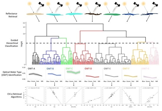
1. Introduction
The turn of the century has seen an apparent increase in the frequency and magnitude of harmful algal blooms in lakes, resulting in significant social, economic, and ecological damage [1,2,3]. It is theorized that the increase in blooms is a result of atmospheric changes (e.g., increased temperatures) and land use changes (e.g., agricultural intensification) [4]. The repercussions of frequent and intense blooms have motivated improved lake sampling efforts; however, there is often a sampling bias towards large lakes close to settled areas, while smaller lakes that scatter remote landscapes are often not sampled [5]. Lakes are regarded as sentinels of change in atmospheric and terrestrial systems, with smaller lakes often having a larger response compared to larger lakes [6,7].
Monitoring of lake algae typically relies on measurements of algal density and biomass or biovolume [8]. While ground-based measurement options provide precise information, remote sensing options are preferable—if not the only ones possible—in remote locations. Remote sensing can be used to provide estimates of chlorophyll-a concentration (chl-a) [9], a proxy for algal biomass because of its unique optical signature and because it is the dominant photosynthetic pigment in most algae [10]. The Landsat satellite series provides the longest available time series of any spaceborne remote sensing system (1982–present), with a spatial resolution (30 m for visible-NIR bands) capable of resolving smaller waterbodies. However, monitoring of lake chl-a with Landsat is limited by a poor signal–noise ratio (particularly with Landsat 5 TM (1984–2013) and 7 ETM+ (effective 1999–2003) sensors), relative to other available satellite sensors (e.g., Landsat 8 OLI (2013–present), Sentinel 3-A (2016–present)), and by wide radiometric bands [11,12]. Despite these limitations, Landsat has a long history of being used as a remote measuring system for chl-a at small spatial and temporal scales [13,14,15,16,17,18,19,20,21,22]. Other remote sensors may be more precise in discerning finer resolution spectral signals; however, because of its long time series, further analysis of Landsat product applicability will be instrumental in predicting historical surface algal biomass.
To compensate for Landsat’s bandwidth limitation, band radiances or reflectances are often multiplied (band products), divided (band ratios), or combined into more complex equations (band combinations), all of which are hereafter referred to as algorithms. Chl-a is commonly identified through combinations of Blue (herein referred to as B) and Green (herein referred to as G) bands [23,24,25,26], B and Red (herein referred to as R) bands [27,28], or G and R bands [29,30,31]. However, chl-a retrieval based on these algorithms often fails to account for interfering signals from non-algal particles [32,33]. Optically active non-algal particles have less influence on absorption or reflectance in the near-infrared (NIR; herein referred to as N) band [34], and many studies have found that the R–N ratio performed best in retrieving chl-a in turbid waters [35,36,37]. Three-band algorithms have also been used for chl-a retrieval in turbid waters, as first described by Gitelson et al. [38,39] and later adapted by Keith et al. [40]. Effective use of these algorithms is, however, limited because the composition and concentration of non-algal particles that interfere with the reflectance properties of water will vary among lakes [41,42,43,44]. The application of a single common algorithm over large spatial extents may therefore increase predictive errors.
To overcome the heterogeneity of freshwater optics, lakes can be separated into optical water types (OWT) by their observed spectra. OWTs serve as a comprehensive classification system, as different limnological conditions in turbid waters return unique spectral signatures [45,46,47]. The separation of observations into OWTs may optimize chl-a retrieval, as algorithm performance depends on the freshwater optics. While hyperspectral imagery provides the most accurate retrieval of spectral profiles for determining OWTs [48,49] (as higher spectral resolution may observe more unique optical signal patterns), studies have shown effective OWT classifications using only six visible and N radiometric bands [44,45,46]. Classification of OWTs using the Landsat satellite series remains difficult, due to the availability of only four visible-N bands.
This study has two research questions as follows: (1) Can lake OWTs be identified using Landsat data without in situ spectra? (2) Does the separation of lakes into OWTs using Landsat data improve the performance of chl-a retrieval algorithms vs. applying those algorithms globally? This study looks to use widely available water quality metrics (chl-a and turbidity) from publicly available data sources to determine ways to optimize chl-a retrieval from limited data. Positive findings to both questions will not only improve the ability of researchers to estimate lake chl-a but may improve monitoring programs, expanding the spatial and temporal range of chl-a estimation across the length of Landsat’s records.
2. Materials and Methods
2.1. Ground-Based Dataset
Ground-based chl-a (μg L−1) and turbidity (NTU) samples taken ≤1 m from the water surface were acquired from various private and public lake water quality databases throughout North America and Fennoscandia, spanning multiple ecoregions (temperate continental forest, steppe, desert, mountain, subtropical humid forest, and tropical moist forest) from July to October (1984–2016) (see Table S1 in the Supplementary Material for more information). Ground-based samples were provided by the Government of British Columbia’s Environmental Monitoring System (EMS) surface water data repository, the USGS Storage and Retrieval (STORET) database, the USGS National Water Information System (NWIS) database, and the Swedish University of Agricultural Science (SLU) Miljödata MVM Environmental database. Samples were selected in these ecoregions as they provided consistent open data sources for lake water quality parameters. These databases also helped provide a geographic spread of data from the tropics to northern temperate ecoregions, which may provide a diverse range of potential water types. Geographic clustering of data occurs as only specific ecoregions had frequently reported water quality results. Only samples where both chl-a and turbidity were taken within ±3 days of a Landsat 4, 5, 7, or 8 satellite overpasses were selected. This window size was chosen to allow for an adequate number of matchups between samples and satellite overpasses while maintaining a relationship with measured reflectance [50]. Limited samples of coloured dissolved organic matter and total suspended solids metrics were found within this window and therefore were not used in this study. A total of 204 sample pairs within 142 lakes were selected (Figure 1, Table S1). Lake sizes ranged from 5.3 to 86,661.9 ha (median = 119.3 ha). Due to a lack of available metadata for public data records, differences in ground-based measurement processing and calibration will occur and offer a source of potential error in the remote sensing retrieval.
2.2. Landsat Image Acquisition, Processing, and Analysis
Sample locations were mapped to the Worldwide Reference System (WRS-2) Landsat catalogue system to identify the (longitudinal) paths and (latitudinal) rows in which the samples were found. A total of 105 pairs of Landsat Level-1 and -2 images with <10% cloud coverage and within ±3 days of sample dates were downloaded from the USGS EarthExplorer data catalogue (https://earthexplorer.usgs.gov/, last accessed: 3 November 2021) (72 Landsat 4-5 TM, 11 Landsat 7 ETM+ (SLC-on), and 22 Landsat 8 OLI) (Table S1).
Various atmospheric correction options are available for the remote sensing of water quality using Landsat data (e.g., 6S, DOS, COST, iCOR); however, such methods often result in errors due to the violation of the dark pixel assumption in turbid waters when estimating aerosol optical thickness in the N [51,52]. While the SWIR band can be used in lieu of the N, it often results in lower aerosol accuracy estimation due to a poorer signal–noise ratio [53]. Some studies have instead opted for simple atmospheric correction of Rayleigh scatter (and not of aerosol contributions) for chl-a retrieval in turbid waters [54,55,56,57,58]. To reduce opportunities for overestimation of atmospheric contributions, this study corrected Landsat data for Rayleigh scatter contribution only.
OWTs were identified from top-of-atmosphere (TOA) reflectance values (0–1) in B (band 1 TM and ETM+, band 2 OLI), G (band 2 TM and ETM+, band 3 OLI), R (band 3 TM and ETM+, band 4 OLI), and N (band 4 TM and EMT+, band 5 OLI) bands. TOA radiance (W ∕ (m2 × sr × µm)), measured by Landsat sensors, were scaled using multiplicative (gain) and additive (bias) scaling factors to 8-bit (0–255; TM and ETM+) and 16-bit (0–65,000; OLI) integer value ranges (digital numbers or DNs) for transmission and storage in Landsat Level-1 products. DNs were recalibrated to TOA radiance using the standard equation [59], as follows:
where L is TOA radiance for wavelength (λ) range or band λ.
TOA radiances were corrected for Rayleigh scatter (attributed to the molecular properties of the atmosphere) using an inverse algorithm based on a simplified radiative transfer model presented by Gilabert [60], as follows:
where Lr is the Rayleigh path radiance for band λ, ESUN is the mean solar exo-atmospheric irradiance for band λ, Pr is the Rayleigh phase function, θs is the solar zenith angle in degrees, θ is the satellite viewing angle in degrees (equal to 0° for Landsat 4, 5, and 7 images and for nadir-looking Landsat 8 images), τr is the Rayleigh optical thickness, and toz↑ and toz↓ are upward and downward ozone transmittance, respectively.
The Rayleigh phase function (Pr) [61,62] describes the angular distribution of scattered light and was calculated as follows:
where Θ is the scattering angle (180° − θs), γ = δ/(2 − δ), and δ is the depolarization factor that denotes the polarization of anisotropic particles at right angles—dependent on the wavelength, atmospheric pressure (constant), and air mass (constant) [63,64].
Ozone transmittance (toz↑ and toz↓) [67] were calculated as follows:
where τoz is the ozone optical thickness, as calculated by [68].
Lr was subtracted from L for each band λ to determine Rayleigh-corrected TOA radiance () as follows:
was then converted to unitless TOA reflectance (ρ; 0–1) for each band λ to avoid issues regarding shifts in the solar zenith angle due to latitude and time of year, as follows:
where d is the Earth–Sun distance in astronomical units.
Lake boundaries were delineated from Level-2 images using the dynamic surface water extent (DSWE) model developed by Jones [69] and adapted by DeVries et al. [70]. Contiguous groups of pixels identified as water by the DSWE model were vectorized without polygon simplification (i.e., lake vector boundaries matched the pixel boundaries), and the vectors were then buffered inwards by 15 m (0.5 pixel width) to minimize the spectral effects of edge pixels where the reflectances of vegetation and shallow depths mix with the reflectance of water. Only buffered lake polygons ≥4.5 ha (50 pixels) were used in this study to further minimize the spectral effects of edge pixels.
In each buffered lake polygon, pixels identified as having a high probability of cloud or cloud shadow in the pixel quality assessment band, provided with Level-2 products, were removed. Because ground-based samples were taken from multiple sources, an assumption of spatial homogeneity in the water chemistry was made due to potential inaccuracies in reported sampling coordinates. To meet this assumption, the standard deviation of ρ in all remaining pixels in each buffered lake polygon was calculated for each visible-N band ρλ; homogeneity is expressed as the sum of the band standard deviations (SSD; [71,72]); and lakes with an arbitrary threshold of SSD larger than the median SSD of all lakes were discarded. While a 3 × 3 or 5 × 5 filter may reduce the effects of homogeneity, some public water quality data may only provide lake coordinates and not sampling coordinates. Filters will not provide adequate smoothing for larger waterbodies, and thus lake averages and SSD thresholds were used.
2.3. Identification of OWTs
OWTs are defined as waters with diverse water chemistry compositions resulting in a wide range of spectral signatures in the visible-N spectrum [73]. Common methods of OWT separation use unsupervised classifiers such as k-means or fuzzy c-means [44,45,46]; however, the small number of Landsat bands limits the number of potential observable spectral signatures. To overcome this limitation, a guided approach was implemented, whereby, the ratio of chl-a:turbidity (Chl:T) was used in addition to ρλ in the visible-N bands in a unsupervised hierarchical clustering method. The use of Chl:T indicates whether the optical signal is influenced by a high biomass presence (high Chl:T) or a low biomass presence (low Chl:T). The hierarchical clustering method was done in R using the “hclust” function found in the base “STATS” package using the “Ward” method. The hierarchical clustering distance values were calculated using the “Canberra” method. Distance is measured as the space (referred to as Euclidian space) between data points in a multivariate dataset, which represents how closely clustered points are. Chl:T and ρλ in the visible-N bands were normalized in R using the “preProcess” function found in the “caret” package, with “scale” selected as the method (i.e., dividing each column by its standard deviation) [74]. To determine the optimal number of classes, an elbow method was used, whereby the total within sums of squares for numbers of clusters from 2 to 24 were calculated using the “fviz_nbclust” function as part of the “factoextra” package in R [75]. A three-point piecewise regression of total within sum of squares vs. number of clusters was fit to determine at which point the increase in clusters no longer significantly reduced the total within sum of squares. Each OWT defined using this method was defined as OWT-Ah or OWT-Bh, etc.
To be applicable to lakes where in situ water chemistry is unknown, a supervised classifier was trained using normalized ρλ in the visible-N bands and the now defined OWTs. A quadratic discriminative analysis (QDA) model was selected as it reduces dimensionality and uses the mean vector of each class to define non-linear boundaries between the defined classes. A random stratified sampling technique was used to select 70% normalized training and 30% normalized testing data using the “stratified” function from the “splitstackshape” package in R (seed = 854) [76]. The QDA was calculated in R using the “qda” function found in the “MASS” package [77]. Each OWT defined using this method is defined as OWT-Aq or OWT-Bq, etc.
2.4. Development of Chl-a Retrieval Algorithms
A total of 82 algorithms—including all possible band products and ratios, as well as commonly used multiband combinations found in the literature (Tables S2 and S3)—were tested for the empirical retrieval of chl-a across all lakes (i.e., global models) and within each OWT using linear regression. Chl-a and turbidity values were log-scaled to meet the assumption of normality. Shapiro–Wilk tests were used to assess the normality (p ≥ 0.05) of relationships between dependent and independent variables. Breusch–Pagan tests were used to assess constant variance (p ≥ 0.05) between dependent and independent variables using the “lmtest” R package [78]. Outliers in selected models were identified using Cook’s distance >4/n prior to regression modelling of chl-a. Algorithm strength and significance were evaluated using coefficients of determination (r2) and regression p-values: these were used to compare the strength and significance (p < 0.05) of correlations between mean lake ρλ to chl-a or turbidity using OWTs vs. global applications. The chl-a retrieval algorithms were validated using ten-fold cross validation and the predictive performance was measured by the root mean squared error (RMSE) as follows:
where is observed as chl-a and is the predicted value. To compare between different groups of varying sample size and different scales of input chl-a, the RMSE were normalized as follows:
where is the standard deviation of the input chl-a. The root mean log squared error (RMSLE) was calculated as follows:
Predictive performance was also measured by the mean absolute error (MAE), calculated as follows:
The median absolute percentage error (MAPE) was calculated as follows:
Bias was calculated as follows:
The MAE, RMSLE, MAE, and bias were calculated using the “metrics” R package [79], while the MAPE was calculated using the “MLmetrics” package [80]. To showcase the application of the OWT and chl-a retrieval algorithms, a testing image was used (Landsat 8 OLI, 15 August 2021, path = 17, row = 29), where per pixel OWT and modelled chl-a are shown.
3. Results
3.1. Identification of OWTs
The number of OWTs was determined using a three-point piecewise regression in R, where the total within sum of squares was calculated using normalized Chl:T and ρλ in the visible-N bands, and which identified three breaks (k = 3, 7, and 11). The first, k = 3, represents too few potential OWTs, while k = 11 resulted in clusters with too few samples for the development of regressions. To maximize the number of OWTs and maintain reasonable sample sizes, k = 7 was identified as the optimal number.
The unsupervised hierarchical clustering method defined which of the lakes belonged to which OWT (Figure 2). Based on lake surface water chemistry (Table 1, Figure 3), OWT-Eh had the highest Chl:T (median = 6.7) with high chl-a (median = 13.7 µg L−1) and low turbidity (median = 1.9 NTU) measurements. While the Chl:T ratio was high, the lakes were relatively dark compared to OWT-Ah, -Bh, and -Ch, but brighter in the B band compared to OWT-Dh, -Fh, and -Gh (Figure 4a). OWT-Ah had the lowest Chl:T (median = 0.5) with low chl-a (median = 4.0 µg L−1) and high turbidity (median = 7.8 NTU) measurements. While optically bright in the B, G, and R bands, OWT-Ah had low ρλ(N) in ranges similar to the optically dark lakes (Figure 4a). OWTs-Bh and -Ch had moderately high Chl:T (median = 4.8 and 4.5, respectively) with a high chl-a (median = 33.6 µg L−1 and 20.2 µg L−1, respectively) and high turbidity (median = 6.7 NTU and 5.0 NTU, respectively) measurements. OWT-Ch returned the highest ρλ of any OWT, with significantly higher N ρλ. Both OWTs-Bh and -Ch had equally high chl-a and turbidity measurements, with OWT-Ch displaying the greatest variance in its distribution compared to any other OWT (Figure 4a). OWT-Dh had a low Chl:T (median = 1.1) with low chl-a (median = 1.3 µg L−1) and low turbidity (median = 1.7 NTU) measurements. OWT-Dh remained optically dark throughout all four visible-N bands, with little variation in ρλ (Figure 4a). OWTs-Fh and -Gh had moderately low Chl:T (median = 2.5 and 3.0, respectively) with low chl-a (median = 3.00 µg L−1 and 2.95 µg L−1, respectively) and low turbidity (median = 1.2 and 1.0 NTU, respectively) measurements. OWT-Gh exhibited the lowest ρλ with the lowest reflectances in the G and R bands. While OWT-Fh shows an even distribution of chl-a and turbidity, OWT-Gh has slightly higher chl-a relative to turbidity.
The supervised QDA method provided a reasonably accurate prediction of OWTs, with a testing accuracy of 75.4% (Figure 5a) and a total accuracy of 80.1% (Figure 5b). OWTs-Bq, -Cq, -Dq, -Eq, and -Gq were reasonably predicted (i.e., ≥60.0%), but OWTs-Aq and -Fq were poorly predicted (≤25%) (Figure 5a). The order of brightness, as represented by mean ρλ(B, G, R, N) in OWTs, identified through the supervised QDA method and the unsupervised hierarchical clustering method, were the same. OWT-Cq was the brightest (mean ρλ(B, G, R, N) = 0.061); followed by OWTs-Aq (mean ρλ(B, G, R, N) = 0.041) and OWTs-Bq (mean ρλ(B, G, R, N) = 0.040); then by OWT-Eq (mean ρλ(B, G, R, N) = 0.028), OWT-Fq (mean ρλ(B, G, R, N) = 0.027), and OWT-Dq (mean ρλ(B, G, R, N) = 0.022); and finally by OWT-Gq, which was the darkest (mean ρλ(B, G, R, N) = 0.017).
The supervised QDA method identified OWTs with comparable water chemistry distributions to those of the unsupervised hierarchical clustering method (Table 1, Figure 6). OWT-Eq had the highest Chl:T (median = 5.1) with high chl-a (median = 8.4 µg L−1) and low turbidity (median = 2.0 NTU) measurements. OWT-Aq had the lowest Chl:T (median = 0.6) with low chl-a (median = 4.7 µg L−1) and high turbidity (median = 9.5 NTU) measurements. OWTs-Bh and OWTs-Ch had moderately high Chl:T (median = 4.8 and 4.9, respectively) with high chl-a (median = 29.3 µg L−1 and 20.9 µg L−1, respectively) and high turbidity (median = 6.0 NTU and 5.0 NTU, respectively) measurements. OWT-Dh had a low Chl:T (median = 1.4) with low chl-a (median = 2.4 µg L−1) and low turbidity (median = 1.0 NTU) measurements. OWTs-Fh and OWTs-Gh had moderately low Chl:T (median = 2.5 and 3.0, respectively) with low chl-a (median = 2.9 µg L−1 and 3.0 µg L−1, respectively) and low turbidity (median = 1.2 and 1.0, NTU, respectively) measurements. When observing the placement of QDA OWTs in the chl-a vs. turbidity plot (Figure 4b), similar results to the hierarchical clustering were found, with the greatest difference in OWT-Dq, which was misclassified with OWTs-Fq and OWTs-Gq.
3.2. OWT Chl-a Retrieval Performance
In the absence of OWT separation, global algorithms demonstrated moderate to poor performances for chl-a retrieval. The [(R/B) × (R/N)] algorithm exhibited the highest r2 (0.52, p < 0.05, n = 147) with the seventh lowest NRMSE and the fourth lowest MAPE out of 82 algorithms in total. Of the 10 algorithms with the highest r2, all included the use of the R band, while 70%, 30%, and 30% included N, G, and B bands, respectively (Table 2), 70% included both the R and N bands, and 40% included a ratio of R and N. Compared with the best performing global algorithm, algorithm performances improved when separated into OWTs using unsupervised hierarchical clustering and supervised QDA. The algorithm performances were similar between OWTs identified by the two methods (Table 3), except for OWTs-C (higher r2 in OWT-Cq), -D (higher r2 in OWT-Dh), -E (higher r2 in OWT-Eh), and -F (higher r2 in OWT-Fq).
Based on Chl:T, OWTs-Ah and OWTs-Dh represent lakes where the chl-a remains relatively low despite higher relative turbidity measurements. In both OWT-Ah and OWTs-Dh, [G × (B + G + R)] and [N/G] had the highest r2 (1.00, p < 0.05, n = 4; 0.97, p < 0.05, n = 9, respectively); however, due to the small sample size after outlier removal, the algorithm with the next highest r2, [B/R], and [G/N] was preferable (r2 = 0.91, p < 0.05, n = 9; r2 = 0.91, p < 0.05, n = 13, respectively). Due to the small sample sizes (n < 10), most error metrics (RMSE, RMSLE, NRMSE, and MAE) were not calculated; however, [B/R] and [G/N] had the 23rd and the 3rd lowest MAPE respectively. In both OWTs, of the ten algorithms with the highest r2, N was included in the largest number. In OWT-Aq, and OWTs-Dq [(R/G) × N] and [R] had the highest r2 (0.91, p < 0.05, n = 5; 0.55, p < 0.05, n = 10, respectively). [(R/G) × N] and [R] had the 7th and 15th lowest MAPE respectively. Of the ten algorithms with the highest r2, N was included in the largest number in OWT-Aq, while G was included in the largest number in OWT-Dq.
Based on Chl:T, OWTs-Bh and OWTs-Ch represent eutrophic lakes where both chl-a and turbidity measurements were relatively high. In both OWT-Bh and OWTs-Ch, [B/G] and [(B/G) × (R/G)] had the highest r2 (0.82, p < 0.05, n = 23; 0.26, p = 0.08, n = 13, respectively), with 2nd and 18th lowest NRMSE and the 7th and 1st lowest MAPE, respectively. Of the ten algorithms with the highest r2, B and N were included in the largest number in OWT-Bh, with G the most frequent in OWT-Ch. Algorithm performances in OWT-Ch, however, were consistently poor. In both OWT-Bq and OWTs-Cq, [(B/G)] and [(B × N)] had the highest r2 (0.85, p < 0.05, n = 26; 0.59, p < 0.05, n = 10), with the 2nd and 1st lowest NRMSE and MAPE respectively. Of the ten algorithms with the highest r2, B, G, and R bands were included in the largest number in OWT-Bq, while B was included in the largest number in OWT-Cq. While OWT-Cq does provide an improvement over OWT-Ch, [(B × N)] was the only algorithm with an adequate performance as the next highest r2 was found for [(B/G) × (R/G)] (r2 = 0.33, p < 0.05, n = 16).
Based on Chl:T, OWT-Eh represents lakes where the turbidity measurements remains relatively low, despite the higher relative chl-a. In OWT-Eh, [B/N] had the highest r2 (0.77, p < 0.05, n = 36), with the 4th lowest NRMSE and the 2nd lowest MAPE. Of the ten algorithms with the highest r2, N was included in the largest number. Conversely, in OWT-Eq, [(B/N)] had the highest r2 (0.47, p < 0.05, n = 56) with the lowest NRMSE and the 8th lowest MAPE. Of the ten algorithms with the highest r2, B was included in the largest number.
Based on Chl:T, OWTs-Fh, and OWTs-Gh represent oligotrophic or mesotrophic lakes, where both chl-a and turbidity measurements are relatively low. In both OWT-Fh and OWTs-Gh, [(G/R) × N] and [(B/G) × (R/N)] had the highest r2 (0.78, p < 0.05, n = 27; 0.69, p < 0.05, n = 21, respectively), with 12th and 1st lowest NRMSE, and the 4th and 44th lowest MAPE respectively. Of the ten algorithms with the highest r2, N was included in the largest number in both OWTs. In OWTs-Fq and -Gq, [G × (B+G+R)] and [(B/G) × (R/N)] had the highest r2 (0.98, p < 0.05, n = 13; 0.68, p < 0.05, n = 24, respectively), with the 1st and 4th lowest NRMSE and the 4th and 29th lowest MAPE respectively. Of the ten algorithms with the highest r2, R was included in the largest number in OWT-Fq, while N was included in the largest number in OWT-Gq.
The described methods identified seven OWTs with unique water chemistry compositions, varying spectral curves, and levels of brightness. The supervised classification returned similar OWTs with similar algorithm performances. In comparison with the global algorithms, separation into OWTs provided significantly improved retrieval accuracy for six of the seven OWTs. Scatter and validation plots for OWTs are presented in Figure 7 and Figure 8, respectively, for unsupervised hierarchical clustering, and in Figure 9 and Figure 10, respectively, for supervised QDA. Full algorithm performance metrics for hierarchical clustering and QDA can be found in Tables S2 and S3, respectively. The application of the OWTs and the subsequent modelling of chl-a can be seen in Figure 11, where a variety of OWTs were retrieved per pixel for several lakes in central–eastern Ontario.
4. Discussion
This study sought to determine the following: whether Landsat-derived ρλ have the capacity to differentiate OWTs with unique spectral signatures and water chemistry distributions; whether OWT-specific algorithms improved chl-a retrieval accuracy compared with that of a global algorithm. Given the limited number of Landsat’s broad radiometric bands, a unsupervised classifier was developed using ρλ in the visible-N bands, guided by Chl:T to produce seven OWTs with both unique spectral signatures and unique water chemistry profiles. A supervised classifier was trained using the guided unsupervised OWTs and applied to lakes where lake surface water chemistry was unknown. The supervised classifier provided reasonably accurate classification results, returning similar chl-a retrieval algorithm performances compared to the guided unsupervised classifier.
4.1. Identifying OWTs
The guided, unsupervised classifier differentiated lakes as optically bright (OWTs-Ah, -Bh, and -Ch) and optically dark (OWTs-Dh, -Eh, -Fh, and -Gh) (Figure 2). However, this classifier also defined OWTs with unique water chemistry distributions. The optically bright lakes had distinct spectral curves, mostly differentiated by Chl:T and the observed ρλ in the N band (Figure 3). Among the optically bright lakes, OWT-Ah represented lakes where ρλ was high with low chl-a. Despite the low biomass, turbidity remained high along with a greater increase in ρλ in the R band and a smaller increase in the N, indicating a potential for non-algal particle dominance in this OWT [33,81]. OWTs-Bh and -Ch represented turbid lakes, as there was a relatively equal ratio of B–G and R–N ρλ. OWT-Bh exhibited notably higher ρλ in the G and R bands compared with OWTs-Dh to -Gh. The increased absorption in the R band due to chl-a was countered by the increase in non-algal particulate scatter, as is often seen in turbid waters. OWT-Ch exhibited much higher ρλ in the N band compared to other OWTs. Additionally, OWT-Ch represented a much wider range of Chl:T values (Figure 3f). Exploration of the metadata showed that the OWT-Ch lakes had the smallest surface area of all OWTs (median = 75.6 ha), suggesting that these lakes may have exhibited high ρλ(N) due to shallow emergent vegetation or shoreline contamination. The optically bright lakes returned significantly brighter G and R bands relative to the B and N bands when compared to the optically dark lakes (with the exception of the N band for OWT-Ch).
The optically dark lakes had similar spectral curves, mostly differentiated by the level of brightness (Figure 2). Among the optically dark lakes, OWT-Dh represented oligotrophic or mesotrophic lakes with low Chl:T where the spectral curve does not replicate that of OWT-Ah, which is likely a result of low chl-a and turbidity measurements where water absorption would dominate the spectra. OWT-Eh represented mesotrophic or eutrophic lakes with high Chl:T and low ρλ in the R band, relative to other bands, as a result of chl-a absorbance [10]. Lakes in which there is a significant spike in ρλ in the N band relative to R suggest that most of the signal is a result of algal particles [81]. Non-algal particles are a significant contributor to backscatter at all wavelengths, but the contribution decreases at higher wavelengths, while algal particles increase backscatter at higher wavelengths [81]. OWTs-Fh and -Gh represented oligotrophic or mesotrophic lakes with low chl-a and turbidity measurements. OWT-Fh represented a more even mix of chl-a and turbidity (i.e., the lakes were closer to the 1:1 line in Figure 4), and resembled the spectral shape of OWT-Bh, though optically darker. OWT-Gh had slightly lower relative turbidity and, therefore, more closely resembled the spectra of OWT-Eh, though optically darker. For lakes classified as optically dark, the B band returned the highest mean lake ρλ, G the second highest, and R the lowest, with a slight increase in the N. The high B band ρλ was likely due to water as the algal particles remained low [48,82]. Typically, N should remain the lowest observed mean lake ρλ; however, due to the atmospheric correction of only Rayleigh scatter used in this study, a higher proportion of observed visible radiance (B, G, and R bands) was removed compared with that of radiance in the N band.
While the guided unsupervised classifier differentiated OWTs based on varying magnitudes of brightness and distinct lake surface water chemistry, it required the water chemistry to be known. The application of the chl-a retrieval algorithm would be used when in situ chl-a and turbidity are unknown; therefore, the supervised classifier is required. The supervised classifier would need to accurately return similar OWTs compared to that of the guided unsupervised classifier, where each OWT returns similar spectra and water chemistry information.
As with the unsupervised classifier, the supervised classifier (QDA) differentiated lakes as optically bright (OWTs-Aq, -Bq, and -Cq) and optically dark (OWTs-Dq, -Eq, -Fq, and -Gq) (Figure 2). The QDA accurately defined the optically bright and dark lakes when comparing the magnitudes of brightness observed (Table 1). OWTs with unique water chemistry distributions were also observed when comparing the Chl:T value of each QDA-derived OWT (Figure 6) to those derived by the unsupervised classifier (Figure 3). OWT specific classification errors do occur particularly for lakes with a low Chla:T, as OWTs-Aq and -Dq returned low classification accuracy. The difficulty in defining OWTs with a low Chla:T may be due to the high variability in the observed ρλ for the visible bands (Figure 3), as the composition of potential non-algal particles (e.g., white vs. red clays) can greatly affect the visible spectra. OWT-Fh had also returned poor classification accuracy, often misclassified as OWT-Eq. The misclassification tended to occur in mesotrophic lakes where chl-a was high. Despite these issues, all other OWTs (i.e., OWTs-Bq, -Cq, -Eq, -Gq) returned high classification accuracy, indicating the supervised classifier is capable of defining OWTs when using Landsat-derived ρλ. The application of Landsat for chl-a retrieval in mixed waters is limited due to its broad radiometric bands [83,84], and this limitation extends to the identification of OWTs. Landsat has the capacity to resolve the difference between optically bright and dark signals with a varying range of Chl:T at the lake level (using mean ρλ in the entire waterbody); however, further resolution is unlikely (i.e., differentiating sediment from detritus material, differentiating algal taxonomy). Additionally, dissolved and particulate matter will increase backscatter and subsequent observed ρλ at visible wavelengths, depending on the composition and concentration [33,85]. The minimal difference in the observed spectra of these lakes is potentially due to the low signal–noise ratio of the Landsat satellite series (particularly with Landsat 5 TM and 7 ETM+), in which small incremental changes in water properties are not likely to be observed in the spectra of dark lakes [12,86]. To define the Chl:T range among varying levels of brightness, the application of lake surface water chemistry parameters in guiding the classification of OWTs offers an improvement when using only Landsat observed ρλ. While in situ spectroradiometers, hyperspectral imagers, and multispectral satellites have a higher number of visible-N bands that may provide more accurate results, the methods outlined in this paper are to be employed when such data are not available.
4.2. OWT Chl-a Retrieval Performance
Eighty-two chl-a retrieval algorithms were tested for each OWT to determine which algorithm performed best. Algorithms performed at varying levels in each OWT, with some patterns observed in the types of bands used. The best performing algorithms using the supervised classifier (i.e., OWTs-Aq, -Bq, etc.) and the guided unsupervised classifier (i.e., OWTs-Ah, -Bh, etc.) were then compared.
OWTs-Ah and -Dh represented a low Chl:T, where OWT-Ah was optically brighter and consisted of higher turbidity measurements. Both OWTs returned high r2 and low overall error; however, some of these fits were inflated due to small sample sizes after outliers were removed. As the chl-a signal was relatively low despite the high brightness observed, a low correlation was expected. The high r2 with algorithms using B and G bands were likely false positives due to the high reflectivity of potential non-algal particles at shorter wavelengths, particularly when chl-a is low [33]. Due to the classification errors with both QDA-derived OWTs (particularly OWT-Aq), the best performing algorithms as indicated by r2 did not match well. The best performing algorithms frequently utilized the R and N bands for OWT-Aq and the G and R bands for OWT-Dq, which is expected for turbid waters. While the performance as measured by r2 did not provide a good match for OWT-Dq, other error metrics such as NRMSE provided a slightly better match, where the same algorithms derived from unsupervised and supervised classifiers had similar retrieval errors.
OWTs-Bh and -Ch represented eutrophic lakes, where both chl-a and turbidity measurements are high relative to the training data distribution. For optically complex and turbid lakes, an R–N ratio is traditionally used [35,36,37]. According to Gitelson [39], this ratio should capture the R edge to N transition (~700 nm), which is currently not possible with Landsat; however, N bands have been used in past studies as an alternative [87]. The best performing algorithms in both OWTs typically used B and G bands, with the best performing algorithms in OWT-Bh also commonly including the N band. Both OWTs returned algorithms using a B–G ratio, which is commonly used for oligotrophic waters due to increased water column penetration, lack of non-algal particles increasing scatter, and highest ρλ in the G band [88]. It is possible that the influence of non-algal particles in OWT-Bh was driving the observed r2. OWT-Ch returned a very poor performance compared to OWTs-Bh, which may reflect the small median lake size, potential emergent vegetation, or shoreline contamination. OWT-Bh provided some algorithms with an adequate performance that would be expected to provide a better chl-a signal in turbid waters, such as [(R/B) × (R/N)], which exhibited the lowest NRMSE and used the R–N ratio (r2 = 0.77, p < 0.05). As the supervised classification accuracy was high, both OWT-Bq and -Cq provided similar algorithm results.
OWT-Eh represented lakes with a high Chl:T, where the turbidity was relatively low given higher relative chl-a. The lakes are considered optically dark, a result of low turbidity, where the signals may be influenced by a lack of non-algal particles increasing ρλ in the B band (due to water reflectance) and decreasing ρλ in the G and R bands; moreover, other factors such as DOM, which typically increases absorption at shorter wavelengths, may not be present as well [89]. The spectra therefore resemble those of other optically dark OWTs, although the brightest of the dark OWTs on average. Algorithms with lower NRMSE use the G–B ratio and the R–N ratio which are commonly used chl-a retrieval metrics [9]. OWT-Eq had returned highly similar algorithms albeit with far poorer performance metrics.
OWTs-Fh and -Gh represented oligotrophic and mesotrophic lakes, where both chl-a and turbidity measurements were low relative to the training data distribution. While the lake surface water chemistry values were low, there was a relatively even distribution of chl-a and turbidity measurements. The best performing algorithms for both OWTs were suited to retrieving chl-a in turbid mixed lakes, with OWT-Fh using a G–R ratio and OWT-Gh using both B–G and R–N ratios. A G–R ratio was used for chl-a retrieval in turbid lakes for other studies similar to the R–N edge, as both implement a maximal absorption and reflectance peaks for chl-a [30]. When classified using the QDA method, similar algorithm performances were found in OWT-Gq in which the best performing algorithm as the same as in -Gh, while OWT-Eq does suffer from misclassification, particularly with OWT-Fh. The misclassification of OWT-Eq with -Fh may explain the improved performance of OWT-Fq, which, as a result, covered a much larger range of chl-a measurements (Table 1), in which higher chl-a often has a stronger observable signal when using Landsat.
4.3. Comparison of Global Algorithms to OWTs
Optically bright lakes exhibited unique algorithm performances, while optically dark lakes returned similar performances with the same algorithms (Figure S1). All OWTs provided unique algorithm performances in comparison to the global models. OWTs consistently had improved retrieval accuracy and lower error (RMSE, NRMSE, RMSLE, and MAE) compared with those of the global algorithms, with the exception of OWT-Ch (Table 3). Instances of global algorithm performance exceeding that of an OWT may also be a result of the following assumptions and methods established within this study. This study used mean ρλ in each lake to identify a singular OWT; however, multiple water types can exist within one lake due to differences in morphology, weather, and land use [47]. The use of a mean ρλ may help in reducing noise in observed ρλ, improving the linear regression at the global level. The use of a mean ρλ, however, may also reduce the capacity for classifiers to define unique spectra, as seen in the optically dark lakes. Lakes—especially large lakes—may represent more than one OWT due to spatial (e.g., multiple lake basins, local point sources of detritus, nutrient, or sediment runoffs; Figure 11) and temporal (e.g., shifts in water chemistry due to precipitation, lake mixing, or algal growth events) factors. Therefore, the separation of OWTs may not provide significant chl-a retrieval performance over that of a global model for lakes that exhibit multiple optical signals prior to outlier removal. When these lakes are placed into OWTs and used in a regression, the variability they introduce is more statistically impactful on the correlation when the sample size is smaller; therefore, the global algorithm is less affected by the variability introduced by this method. Additional variability will also be introduced due to the effects of atmospheric aerosol contribution.
This study made use of simple empirical algorithms such as band ratios and combinations. Bio-optical models [90], such as water colour simulator (WASI) [91], have shown promising results for chl-a retrieval in optically complex waters [92]. However, these physics-based models require knowledge of the absorption and backscatter of IOPs, which were not available in public water quality data records and were, therefore, not employed in this study. Additionally, various bio-optical models require specifically centred bands which are not provided for by Landsat and require spectral calibration using in situ reflectances [93]. Alternative empirical methods such as machine learning, Empirical Orthogonal Function (EOF) analysis, and line-height algorithms options may also provide improvement to chl-a retrieval in optically complex waters [7,90,91,94]. Machine learning methods such as artificial neural networks require significant training data for accurate results [95]. The separation of data into OWTs limits the available training and testing data; therefore, a machine learning approach was not appropriate for this study. EOF is a type of principle component analysis that is not commonly used for chl-a retrieval but has shown potential in some studies [96]. Line-height algorithms typically use chl-a fluorescence peaks at which Landsat bands are not centred. New methods such as colour space transformations have been applied to improve chl-a retrieval [97,98] by converting a multiband RGB to a hyper–hue–saturation–intensity image [99]. While this study looked to improve upon traditional band algorithms, colour space transformation may be an optimal method to use in future studies. Future studies may also look to integrate externally derived OWTs using more refined techniques [47,100] to improve upon OWT identification in Landsat imagery.
5. Conclusions
There has been an increase in the number of algal bloom reports in lakes, for which remote sensing retrieval of chl-a for small inland waters is needed to develop a predictive understanding of algal bloom occurrence. Landsat provides the largest historical image record of any sensor and has a long history of chl-a retrieval. This study showed that a guided OWT classification system using Landsat normalized ρλ and Chl:T to define OWTs provided significant improvements in chl-a retrieval algorithms. Seven OWTs based on ρλ in Landsat visible-N bands and on Chl:T were able to retrieve chl-a for inland lakes ranging from eutrophic to oligotrophic, and from turbid to clear, with significantly improved accuracy compared to a global chl-a retrieval algorithms. The separation of lakes into OWTs did improve chl-a retrieval, including in areas where algal blooms occur within less frequently studied, but equally important, lakes. Future work should focus on seeing if the performance of Landsat data for identifying OWTs and predicting chl-a could be further improved by improving supervised classification techniques, and by implementing additional water chemistry data that may help in further differentiating distinct OWTs.
Supplementary Materials
The following are available online at https://0-www-mdpi-com.brum.beds.ac.uk/article/10.3390/rs13224607/s1, Figure S1: Pearson correlation (r) matrix of chl-a retrieval algorithms performance results, Table S1: Ground-based water chemistry samples, corresponding images, and source summary, Table S2: Chl-a retrieval algorithm results summary for OWTs-Ah–Gh, Table S3: Chl-a retrieval algorithm results summary for OWTs-Aq–Gq, Spreadsheet 1: Optical water type spectral and water quality data.
Author Contributions
The authors M.A.D. and I.F.C. have contributed significantly to the research presented in this paper in the following sections: conceptualization, M.A.D. and I.F.C.; methodology, M.A.D. and I.F.C.; software, M.A.D.; validation, M.A.D.; formal analysis, M.A.D.; investigation, M.A.D.; resources, M.A.D.; data curation, M.A.D.; writing—original draft preparation, M.A.D. and I.F.C.; writing—review and editing, M.A.D. and I.F.C.; visualization, M.A.D.; supervision, I.F.C.; project administration, I.F.C.; funding acquisition, I.F.C. All authors have read and agreed to the published version of the manuscript.
Funding
This research was funded by Natural Sciences and Engineering Research Council of Canada (NSERC) Discovery Grant 06579-2014 and an NSERC Collaborative Re-search and Training Experience (CREATE) Grant 448172-2014 to Irena F. Creed.
Data Availability Statement
This research utilized publicly available water quality data from the following sources: The Government of British Columbia (2021) Environmental Monitoring System (EMS) Surface water monitoring. Last accessed 3 November 2021 at URL https://www2.gov.bc.ca/gov/content/environment/research-monitoring-reporting/monitoring/environmental-monitoring-system. U.S. Geological Survey (2021), Environmental Protection Agency: Storage and Retrieval (STORET). Data available on the World Wide Web (USGS Water Data for the Nation). Last accessed 3 November 2021 at URL https://www.waterqualitydata.us/portal AND U.S. Geological Survey (2021), National Water Information System (NWIS). Data available on the World Wide Web (USGS Water Data for the Nation). Last accessed 3 November 2021 at URL https://www.waterqualitydata.us/portal/. Swedish University of Agricultural Sciences (SLU) (2021). Miljödata MVM Environ-mental Data. Last accessed 3 November 2021 at URL http://miljodata.slu.se/mvm.
Acknowledgments
We would like to thank the NSERC DG and CREATE Algal Bloom Assessment through Technology and Education (ABATE) program for funding the research, Ben DeVries for the contribution of his DSWE script for the classification of in-land waterbodies, and David Aldred for his contribution to editing the text and figures.
Conflicts of Interest
The authors declare no conflict of interest.
References
- Anderson, D. HABs in a changing world: A perspective on harmful algal blooms, their impacts, and research and management in a dynamic era of climactic and environmental change. In Harmful Algae 2012: Proceedings of the 15th International Conference on Harmful Algae: 2012, CECO, Changwon, Gyeongnam, Korea; Kim, H.-G., Reguera, B., Hallegraeff, G.M., Chang Kyu Lee, M., Eds.; NIH Public Access: Bethesda, MD, USA, 2012; Volume 2012, p. 3. [Google Scholar]
- Pick, F.R. Blooming algae: A Canadian perspective on the rise of toxic cyanobacteria. Can. J. Fish Aquat. Sci. 2016, 73, 1149–1158. [Google Scholar] [CrossRef] [Green Version]
- Winter, J.G.; DeSellas, A.M.; Fletcher, R.; Heintsch, L.; Morley, A.; Nakamoto, L.; Utsumi, K. Algal blooms in Ontario, Canada: Increases in reports since 1994. Lake Reserv. Manag. 2011, 27, 107–114. [Google Scholar] [CrossRef] [Green Version]
- Reid, A.J.; Carlson, A.K.; Creed, I.F.; Eliason, E.J.; Gell, P.A.; Johnson, P.T.; Kidd, K.A.; MacCormack, T.J.; Olden, J.D.; Ormerod, S.J.; et al. Emerging threats and persistent conservation challenges for freshwater biodiversity. Biol. Rev. 2019, 94, 849–873. [Google Scholar] [CrossRef] [PubMed] [Green Version]
- Biggs, J.; von Fumetti, S.; Kelly-Quinn, M. The importance of small waterbodies for biodiversity and ecosystem services: Implications for policy makers. Hydrobiologia 2017, 793, 3–39. [Google Scholar] [CrossRef]
- Adrian, R.; O’Reilly, C.M.; Zagarese, H.; Baines, S.B.; Hessen, D.O.; Keller, W.; Livingstone, D.M.; Sommaruga, R.; Straile, D.; Van Donk, E.; et al. Lakes as sentinels of climate change. Limnol. Oceanogr. 2009, 54, 2283–2297. [Google Scholar] [CrossRef]
- Vinnå, L.R.; Medhaug, I.; Schmid, M.; Bouffard, D. The vulnerability of lakes to climate change along an altitudinal gradient. Commun. Earth Env. 2021, 2, 1–10. [Google Scholar] [CrossRef]
- Suthers, I.M.; Rissik, D.S.; Richardson, A. Plankton: A Guide to Their Ecology and Monitoring for Water Quality, 2nd ed.; CRC Press, Taylor & Francis Group: Boca Raton, FL, USA, 2019. [Google Scholar]
- Matthews, M.W. A current review of empirical procedures of remote sensing in inland and near-coastal transitional waters. Int. J. Remote Sens. 2011, 32, 6855–6899. [Google Scholar] [CrossRef]
- Ogashawara, I.; Mishra, D.R.; Gitelson, A.A. Remote Sensing of Inland Waters: Background and Current State-of-the-Art. In Bio-Optical Modeling and Remote Sensing of Inland Waters; Elsevier: Amsterdam, The Netherlands, 2017. [Google Scholar] [CrossRef]
- Gower, J.F.R.; Borstad, G.A. On the potential of MODIS and MERIS for imaging chlorophyll fluorescence from space. Int. J. Remote Sens. 2004, 25, 1459–1464. [Google Scholar] [CrossRef]
- Schott, J.R.; Gerace, A.; Woodcock, C.E.; Wang, S.; Zhu, Z.; Wynne, R.H.; Blinn, C.E. The impact of improved signal-to-noise ratios on algorithm performance: Case studies for Landsat class instruments. Remote Sens. Environ. 2016, 185, 37–45. [Google Scholar] [CrossRef] [Green Version]
- Boland, D.H.P. Trophic classification of lakes using Landsat-1 (ERTS-1) multispectral scanner data. U.S. In Environmental Protection Agency, Assessment and Criteria Development Division Corvallis Environmental Research Laboratory; National Technical Information Service (NTIS): Springfield, VA, USA, 1975. [Google Scholar]
- Almanza, E.; Melack, J.M. Chlorophyll differences in Mono Lake (California) observable on Landsat imagery. Hydrobiologia 1985, 122, 13–17. [Google Scholar] [CrossRef]
- Ritchie, J.C.; Cooper, C.M.; Schiebe, F.R. The relationship of MSS and TM digital data with suspended sediments, chlorophyll, and temperature in Moon Lake, Mississippi. Remote Sens. Environ. 1990, 33, 137–148. [Google Scholar] [CrossRef]
- Mayo, M.; Gitelson, A.; Yacobi, Y.Z.; Ben-Avraham, Z. Chlorophyll distribution in lake Kinneret determined from Landsat Thematic Mapper data. Int. J. Remote Sens. 1995, 16, 175–182. [Google Scholar] [CrossRef]
- Brivio, P.A.; Giardino, C.; Zilioli, E. Determination of chlorophyll concentration changes in Lake Garda using an image-based radiative transfer code for Landsat TM images. Int. J. Remote Sens. 2001, 22, 487–502. [Google Scholar] [CrossRef]
- Duan, H.; Zhang, Y.; Zhang, B.; Song, K.; Wang, Z. Assessment of chlorophyll-a concentration and trophic state for Lake Chagan using Landsat TM and field spectral data. Environ. Monit. Assess. 2007, 129, 295–308. [Google Scholar] [CrossRef] [PubMed]
- Chen, J.; Wen, Z.; Xiao, Z. Spectral geometric triangle properties of chlorophyll-a inversion in Taihu Lake based on TM data. J. Water Resour. Prot. 2011, 3, 67–75. [Google Scholar] [CrossRef] [Green Version]
- Theologou, I.; Patelaki, M.; Karantzalos, K. Can single empirical algorithms accurately predict inland shallow water quality status from high resolution, multi-sensor, multi-temporal satellite data? Int. Arch. Photogramm. Remote Sens. Spat. Inf. Sci. 2015, 40, 1511. [Google Scholar] [CrossRef] [Green Version]
- Chen, Q.; Huang, M.; Bai, K.; Li, X. An Optimal Two Bands Ratio Model to Monitor Chlorophyll-a in Urban Lake Using Landsat 8 Data. In E3S Web of Conferences; EDP Sciences: Les Ulis, France, 2020; Volume 143, p. 02003. [Google Scholar]
- Paltsev, A.; Creed, I.F. Are Northern Lakes in Relatively Intact Temperate Forests Showing Signs of Increasing Phytoplankton Biomass? Ecosystems 2021, 1–29. [Google Scholar] [CrossRef]
- Carder, K.L.; Chen, F.R.; Cannizzaro, J.P.; Campbell, J.W.; Mitchell, B.G. Performance of the MODIS semi-analytical ocean color algorithm for chlorophyll-a. Adv. Space Res. 2004, 33, 1152–1159. [Google Scholar] [CrossRef]
- O’Reilly, J.E.; Maritorena, S.; Mitchell, B.G.; Siegel, D.A.; Carder, K.L.; Garver, S.A.; Kahru, M.; McClain, C. Ocean color chlorophyll algorithms for SeaWiFS. J. Geophys. Res.-Oceans. 1998, 103, 24937–24953. [Google Scholar] [CrossRef] [Green Version]
- Salem, S.I.; Higa, H.; Kim, H.; Kobayashi, H.; Oki, K.; Oki, T. Assessment of chlorophyll-a algorithms considering different trophic statuses and optimal bands. Sensors 2017, 17, 1746. [Google Scholar] [CrossRef] [PubMed] [Green Version]
- Sudheer, K.P.; Chaubey, I.; Garg, V. Lake water quality assessment from Landsat thematic mapper data using neural network: An approach to optimal band combination selection. J. Am. Water Resour. Assoc. 2006, 42, 1683–1695. [Google Scholar] [CrossRef]
- Han, L.; Jordan, K. Estimating and mapping chlorophyll a concentration in Pensacola Bay, Florida using Landsat ETM data. Int. J. Remote Sens. 2005, 26, 5245–5254. [Google Scholar] [CrossRef]
- Sass, G.; Creed, I.F.; Bayley, S.E.; Devito, K.J. Understanding variation in trophic status of lakes on the Boreal Plain: A 20 year retrospective using Landsat TM imagery. Remote Sens. Environ. 2007, 109, 127–141. [Google Scholar] [CrossRef]
- Brezonik, P.; Menken, K.D.; Bauer, M. Landsat-based remote sensing of lake water quality characteristics, including chlorophyll and colored dissolved organic matter (CDOM). Lake Reserv. Manag. 2005, 21, 373–382. [Google Scholar] [CrossRef]
- Ha, N.; Thao, N.; Koike, K.; Nhuan, M. Selecting the best band ratio to estimate chlorophyll-a concentration in a tropical freshwater lake using sentinel 2A images from a case study of Lake Ba Be (Northern Vietnam). ISPRS Int. J. Geo.-Inf. 2017, 6, 290. [Google Scholar] [CrossRef]
- Moses, W.J.; Gitelson, A.A.; Berdnikov, S.; Povazhnyy, V. Estimation of chlorophyll-a concentration in case II waters using MODIS and MERIS data—successes and challenges. Environ. Res. Lett. 2009, 4, 045005. [Google Scholar] [CrossRef] [Green Version]
- Olmanson, L.G.; Brezonik, P.L.; Finlay, J.C.; Bauer, M.E. Comparison of Landsat 8 and Landsat 7 for regional measurements of CDOM and water clarity in lakes. Remote Sens. Environ. 2016, 185, 119–128. [Google Scholar] [CrossRef]
- Schalles, J.F. Optical remote sensing techniques to estimate phytoplankton chlorophyll a concentrations in coastal. In Remote Sensing of Aquatic Coastal Ecosystem Processes; Richardson, L., LeDrew, E., Eds.; Springer: Dordrecht, The Netherlands, 2006; pp. 27–79. [Google Scholar]
- Gitelson, A.A.; Schalles, J.F.; Hladik, C.M. Remote chlorophyll-a retrieval in turbid, productive estuaries: Chesapeake Bay case study. Remote Sens. Environ. 2007, 109, 464–472. [Google Scholar] [CrossRef]
- Dall’Olmo, G.; Gitelson, A.A.; Rundquist, D.C. Towards a unified approach for remote estimation of chlorophyll-a in both terrestrial vegetation and turbid productive waters. Geophys. Res. Lett. 2003, 30. [Google Scholar] [CrossRef] [Green Version]
- Han, L.; Rundquist, D.C.; Liu, L.L.; Fraser, R.N.; Schalles, J.F. The spectral responses of algal chlorophyll in water with varying levels of suspended sediment. Int. J. Remote Sens. 1994, 15, 3707–3718. [Google Scholar] [CrossRef]
- Singh, K.; Ghosh, M.; Sharma, S.R.; Kumar, P. Blue-red-NIR model for chlorophyll-α retrieval in hypersaline-alkaline water using Landsat ETM+ sensor. IEEE J. Sel. Top. Appl. 2014, 7, 3553–3559. [Google Scholar] [CrossRef]
- Gitelson, A.A.; Gritz, Y.; Merzlyak, M.N. Relationships between leaf chlorophyll content and spectral reflectance and algorithms for non-destructive chlorophyll assessment in higher plant leaves. J. Plant Physiol. 2003, 160, 271–282. [Google Scholar] [CrossRef] [PubMed]
- Gitelson, A.A.; Gao, B.C.; Li, R.R.; Berdnikov, S.; Saprygin, V. Estimation of chlorophyll-a concentration in productive turbid waters using a Hyperspectral Imager for the Coastal Ocean—the Azov Sea case study. Environ. Res. Lett. 2011, 6, 024023. [Google Scholar] [CrossRef]
- Keith, D.; Rover, J.; Green, J.; Zalewsky, B.; Charpentier, M.; Thursby, G.; Bishop, J. Monitoring algal blooms in drinking water reservoirs using the Landsat-8 operational land imager. Int. J. Remote Sens. 2018, 39, 2818–2846. [Google Scholar] [CrossRef] [PubMed]
- Lin, S.; Qi, J.; Jones, J.R.; Stevenson, R.J. Effects of sediments and coloured dissolved organic matter on remote sensing of chlorophyll-a using Landsat TM/ETM+ over turbid waters. Int. J. Remote Sens. 2018, 39, 1421–1440. [Google Scholar] [CrossRef]
- Lymburner, L.; Botha, E.; Hestir, E.; Anstee, J.; Sagar, S.; Dekker, A.; Malthus, T. Landsat 8: Providing continuity and increased precision for measuring multi-decadal time series of total suspended matter. Remote Sens. Environ. 2016, 185, 108–118. [Google Scholar] [CrossRef]
- Ma, J.; Song, K.; Wen, Z.; Zhao, Y.; Shang, Y.; Fang, C.; Du, J. Spatial distribution of diffuse attenuation of photosynthetic active radiation and its main regulating factors in Inland Waters of Northeast China. Remote Sens. 2016, 8, 964. [Google Scholar] [CrossRef] [Green Version]
- Moore, T.S.; Campbell, J.W.; Feng, H. A fuzzy logic classification scheme for selecting and blending satellite ocean color algorithms. IEEE Trans. Geosci. Remote Sens. 2001, 39, 1764–1776. [Google Scholar] [CrossRef]
- Moore, T.S.; Campbell, J.W.; Dowell, M.D. A class-based approach to characterizing and mapping the uncertainty of the MODIS ocean chlorophyll product. Remote Sens. Environ. 2009, 113, 2424–2430. [Google Scholar] [CrossRef]
- Jackson, T.; Sathyendranath, S.; Mélin, F. An improved optical classification scheme for the Ocean Colour Essential Climate Variable and its applications. Remote Sens. Environ. 2017, 203, 152–161. [Google Scholar] [CrossRef]
- Spyrakos, E.; O’Donnell, R.; Hunter, P.D.; Miller, C.; Scott, M.; Simis, S.G.H.; Tyler, A.N. Optical types of inland and coastal waters. Limnol. Oceanogr. 2018, 63, 846–870. [Google Scholar] [CrossRef] [Green Version]
- Moore, T.S.; Dowell, M.D.; Bradt, S.; Verdu, A.R. An optical water type framework for selecting and blending retrievals from bio-optical algorithms in lakes and coastal waters. Remote Sens. Environ. 2014, 143, 97–111. [Google Scholar] [CrossRef] [PubMed] [Green Version]
- Tarabalka, Y.; Chanussot, J.; Benediktsson, J.A. Segmentation and classification of hyperspectral images using watershed transformation. Pattern Recognit. 2010, 43, 2367–2379. [Google Scholar] [CrossRef] [Green Version]
- Olmanson, L.G.; Bauer, M.E.; Brezonik, P.L. A 20-year landsat water clarity census of Minnesota’s 10,000 lakes. Remote Sens. Environ. 2008, 112, 4086–4097. [Google Scholar] [CrossRef]
- Siegel, D.A.; Wang, M.; Maritorena, S.; Robinson, W. Atmospheric correction of satellite ocean color imagery: The black pixel assumption. Appl. Opt. 2000, 39, 3582. [Google Scholar] [CrossRef]
- Ilori, C.O.; Pahlevan, N.; Knudby, A. Analyzing performances of different atmospheric correction techniques for Landsat 8: Application for coastal remote sensing. Remote Sens. 2019, 11, 469. [Google Scholar] [CrossRef] [Green Version]
- Bi, S.; Li, Y.; Wang, Q.; Lyu, H.; Liu, G.; Zheng, Z.; Du, C.; Mu, M.; Xu, J.; Lei, S.; et al. Inland water atmospheric correction based on turbidity classification using OLCI and SLSTR synergistic observations. Remote Sens. 2018, 10, 1002. [Google Scholar] [CrossRef] [Green Version]
- Matthews, M.W.; Bernard, S.; Robertson, L. An algorithm for detecting trophic status (chlorophyll-a), cyanobacterial-dominance, surface scums and floating vegetation in inland and coastal waters. Remote Sens. Environ. 2012, 124, 637–652. [Google Scholar] [CrossRef]
- Matthews, M.W.; Odermatt, D. Improved algorithm for routine monitoring of cyanobacteria and eutrophication in inland and near-coastal waters. Remote Sens. Environ. 2015, 156, 374–382. [Google Scholar] [CrossRef]
- Zhang, Y.; Ma, R.; Duan, H.; Loiselle, S.; Zhang, M.; Xu, J. A novel MODIS algorithm to estimate chlorophyll a concentration in eutrophic turbid lakes. Ecol. Indic. 2016, 69, 138–151. [Google Scholar] [CrossRef]
- Tao, M.; Duan, H.; Cao, Z.; Loiselle, S.A.; Ma, R. A Hybrid EOF Algorithm to Improve MODIS Cyanobacteria Phycocyanin Data Quality in a Highly Turbid Lake: Bloom and Nonbloom Condition. IEEE J. Sel. Top. Appl. 2017, 10, 4430–4444. [Google Scholar] [CrossRef]
- Pahlevan, N.; Smith, B.; Schalles, J.; Binding, C.; Cao, Z.; Ma, R.; Alikas, K.; Kangro, K.; Gurlin, D.; Hà, N.; et al. Seamless retrievals of chlorophyll-a from Sentinel-2 (MSI) and Sentinel-3 (OLCI) in inland and coastal waters: A machine-learning approach. Remote Sens. Environ. 2020, 240, 111604. [Google Scholar] [CrossRef]
- Chander, G.; Markham, B. Revised Landsat-5 TM radiometric calibration procedures and post calibration dynamic ranges. IEEE Trans. Geosci. Remote 2003, 41, 2674–2677. [Google Scholar] [CrossRef] [Green Version]
- Gilabert, M.A.; Conese, C.; Maselli, F. An atmospheric correction method for the automatic retrieval of surface reflectances from TM images. Int. J. Remote Sens. 1994, 15, 2065–2086. [Google Scholar] [CrossRef]
- Chandrasekhar, S. Radiative Transfer; Dover Publications: New York, NY, USA, 1960. [Google Scholar]
- Vermote, E.; Tanré, D.; Deuzé, J.L.; Herman, M.; Morcrette, J.J.; Kotchenova, S.Y. Second Simulation of a Satellite Signal in the Solar Spectrum-Vector (6SV); 6s User Guide Version 3; Laboratoire d’Optique Atmosphérique: Villeneuve d’Ascq, France, 2006; pp. 1–55. [Google Scholar]
- Young, A.T. Revised depolarization corrections for atmospheric extinction. Appl. Opt. 1980, 19, 3427. [Google Scholar] [CrossRef]
- Bucholtz, A. Rayleigh-scattering calculations for the terrestrial atmosphere. Appl. Opt. 1995, 34, 2765. [Google Scholar] [CrossRef]
- Bodhaine, B.A.; Wood, N.B.; Dutton, E.G.; Slusser, J.R. On Rayleigh optical depth calculations. J. Atmos. Ocean. Technol. 1999, 16, 1854–1861. [Google Scholar] [CrossRef]
- Hansen, J.E.; Travis, L.D. Light scattering in planetary atmospheres. Space Sci. Rev. 1974, 16, 527–610. [Google Scholar] [CrossRef]
- Sturm, B. The atmospheric correction of remotely sensed data and the quantitative determination of suspended matter in marine water surface layers. In Remote Sensing in Meteorology, Oceanography and Hydrology; Cracknell, A.P., Ed.; Ellis Horwood Limited: Chichester, UK, 1981; Chapter 11. [Google Scholar]
- Jorge, D.; Barbosa, C.; De Carvalho, L.; Affonso, A.G.; Lobo, F.; Novo, E. SNR (signal-to-noise ratio) impact on water constituent retrieval from simulated images of optically complex amazon lakes. Remote Sens. 2017, 9, 644. [Google Scholar] [CrossRef] [Green Version]
- Jones, J.W. Efficient wetland surface water detection and monitoring via Landsat: Comparison with in situ data from the Everglades Depth Estimation Network. Remote Sens. 2015, 7, 12503–12538. [Google Scholar] [CrossRef] [Green Version]
- DeVries, B.; Huang, C.; Lang, M.; Jones, J.; Huang, W.; Creed, I.; Carroll, M. Automated quantification of surface water inundation in wetlands using optical satellite imagery. Remote Sens. 2017, 9, 807. [Google Scholar] [CrossRef] [Green Version]
- Hou, Z.; Xu, Q.; Nuutinen, T.; Tokola, T. Remote Sensing of Environment Extraction of remote sensing-based forest management units in tropical forests. Remote Sens. Environ. 2013, 130, 1–10. [Google Scholar] [CrossRef]
- Song, Y.; Qu, J. Real time segmentation of remote sensing images with a combination of clustering and Bayesian approaches. J. Real Time Image Process. 2020, 18, 1541–1554. [Google Scholar] [CrossRef]
- da Silva, E.F.F.; de Moraes Novo, E.M.L.; de Lucia Lobo, F.; Barbosa, C.C.F.; Noernberg, M.A.; da Silva Rotta, L.H.; Cairo, C.T.; Maciel, D.A.; Júnior, R.F. Optical water types found in Brazilian waters. Limnology 2021, 22, 57–68. [Google Scholar] [CrossRef]
- Kuhn, M.; Wing, J.; Weston, S.; Williams, A.; Keefer, C.; Engelhardt, A.; Cooper, T.; Mayer, Z.; Kenkel, B.; Team, R.C.; et al. Package ‘caret’. R J. 2021, 223. Available online: https://github.com/topepo/caret/ (accessed on 3 November 2021).
- Kassambara, A.; Mundt, F. Package ‘factoextra’. Extract and Visualize the Results of Multivariate Data Analyses. 2020. Available online: http://www.sthda.com/english/rpkgs/factoextra (accessed on 3 November 2021).
- Mahto, A. Package ‘splitstackshape’. 2019. Available online: https://github.com/topepo/caret/ (accessed on 3 November 2021).
- Ripley, B.; Venables, B.; Bates, D.M.; Hornik, K.; Gebhardt, A.; Firth, D.; Ripley, M.B. Package ‘mass’. Cran R 2013, 538, 113–120. Available online: http://www.stats.ox.ac.uk/pub/MASS4/ (accessed on 3 November 2021).
- Hothorn, T.; Zeileis, A.; Farebrother, R.W.; Cummins, C.; Millo, G.; Mitchell, D.; Zeileis, M.A. Package ‘lmtest’. Testing linear regression models. Cran R 2002, 2, 7–10. Available online: https://CRAN.R-project.org/package=lmtest (accessed on 3 November 2021).
- Hamner, B.; Frasco, M.; LeDell, E. Metrics: Evaluation Metrics for Machine Learning. 2018. Available online: https://github.com/mfrasco/Metrics (accessed on 3 November 2021).
- Yan, Y. MLmetrics: Machine Learning Evaluation Metrics. 2016. Available online: http://github.com/yanyachen/MLmetrics/issues (accessed on 3 November 2021).
- Sun, D.; Li, Y.; Wang, Q.; Lv, H.; Le, C.; Huang, C.; Gong, S. Partitioning particulate scattering and absorption into contributions of phytoplankton and non-algal particles in winter in Lake Taihu (China). Hydrobiologia 2010, 644, 337–349. [Google Scholar] [CrossRef]
- Watanabe, S.; Vincent, W.F.; Reuter, J.; Hook, S.J.; Schladow, S.G. A quantitative blueness index for oligotrophic waters: Application to Lake Tahoe, California-Nevada. Limnol. Oceanogr. 2016, 14, 100–109. [Google Scholar] [CrossRef]
- Kuhn, C.; de Matos Valerio, A.; Ward, N.; Loken, L.; Sawakuchi, H.O.; Kampel, M.; Butman, D. Performance of Landsat-8 and Sentinel-2 surface reflectance products for river remote sensing retrievals of chlorophyll-a and turbidity. Remote Sens. Environ. 2019, 224, 104–118. [Google Scholar] [CrossRef] [Green Version]
- Olmanson, L.G.; Brezonik, P.L.; Bauer, M.E. Evaluation of medium to low resolution satellite imagery for regional lake water quality assessments. Water Resour. Res. 2011, 47, 1–14. [Google Scholar] [CrossRef] [Green Version]
- Han, L. Spectral reflectance with varying suspended sediment concentrations in clear and algae-laden waters. Photogramm. Eng. Remote Sens. 1997, 63, 701–705. [Google Scholar]
- Pahlevan, N.; Balasubramanian, S.V.; Sarkar, S.; Franz, B.A. Toward long-term aquatic science products from heritage Landsat missions. Remote Sens. 2018, 10, 1337. [Google Scholar] [CrossRef] [Green Version]
- Uudeberg, K.; Ansko, I.; Põru, G.; Ansper, A.; Reinart, A. Using optical water types to monitor changes in optically complex inland and coastal waters. Remote Sens. 2019, 11, 2297. [Google Scholar] [CrossRef] [Green Version]
- Mascarenhas, V.; Keck, T. Marine Optics and Ocean Color Remote Sensing. In YOUMARES 8–Oceans across Boundaries: Learning from Each Other; Springer: Cham, Switzerland, 2019; pp. 41–54. [Google Scholar]
- Slonecker, E.T.; Jones, D.K.; Pellerin, B.A. The new Landsat 8 potential for remote sensing of colored dissolved organic matter (CDOM). Mar. Pollut. Bull. 2016, 107, 518–527. [Google Scholar] [CrossRef]
- Simis, S.G.H.; Peters, S.W.M.; Gons, H.J. Remote sensing of the cyanobacterial pigment phycocyanin in turbid inland water. Limnol. Oceanogr. 2005, 50, 237–245. [Google Scholar] [CrossRef]
- Dörnhöfer, K.; Göritz, A.; Gege, P.; Pflug, B.; Oppelt, N. Water constituents and water depth retrieval from Sentinel-2A—A first evaluation in an oligotrophic lake. Remote Sens. 2016, 8, 941. [Google Scholar] [CrossRef] [Green Version]
- Maier, P.M.; Keller, S.; Hinz, S. Deep Learning with WASI Simulation Data for Estimating Chlorophyll a Concentration of Inland Water Bodies. Remote Sens. 2021, 13, 718. [Google Scholar] [CrossRef]
- Manuel, A.; Blanco, A.C.; Tamondong, A.M.; Jalbuena, R.; Cabrera, O.; Gege, P. Optmization of Bio-Optical Model Parameters for Turbid Lake Water Quality Estimation Using Landsat 8 and WASI-2D. Int. Arch. Photogramm. Remote Sens. Spat. Inf. Sci. 2020, 42, 67–72. [Google Scholar] [CrossRef] [Green Version]
- Ioannou, I.; Zhou, J.; Gilerson, A.; Gross, B.; Moshary, F.; Ahmed, S. New algorithm for MODIS chlorophyll fluorescence height retrieval: Performance and comparison with the current product. In Remote Sensing of the Ocean, Sea Ice, and Large Water Regions 2009; International Society for Optics and Photonics: Bellingham, WA, USA, 2009; Volume 7473, p. 747309. [Google Scholar]
- Gholizadeh, M.H.; Melesse, A.M.; Reddi, L. A comprehensive review on water quality parameters estimation using remote sensing techniques. Sensors 2016, 16, 1298. [Google Scholar] [CrossRef] [Green Version]
- Qi, L.; Hu, C.; Duan, H.; Barnes, B.B.; Ma, R. An EOF-based algorithm to estimate chlorophyll a concentrations in Taihu Lake from MODIS land-band measurements: Implications for near real-time applications and forecasting models. Remote Sens. 2014, 6, 10694–10715. [Google Scholar] [CrossRef] [Green Version]
- Mansaray, A.S.; Dzialowski, A.R.; Martin, M.E.; Wagner, K.L.; Gholizadeh, H.; Stoodley, S.H. Comparing PlanetScope to Landsat-8 and Sentinel-2 for Sensing Water Quality in Reservoirs in Agricultural Watersheds. Remote Sens. 2021, 13, 1847. [Google Scholar] [CrossRef]
- Niroumand-Jadidi, M.; Bovolo, F.; Bruzzone, L. Novel spectra-derived features for empirical retrieval of water quality parameters: Demonstrations for OLI, MSI, and OLCI Sensors. IEEE Trans. Geosci. Remote Sens. 2019, 57, 10285–10300. [Google Scholar] [CrossRef]
- Liu, H.; Lee, S.H.; Chahl, J.S. Transformation of a high-dimensional color space for material classification. J. Opt. Soc. Am. 2017, 34, 523–532. [Google Scholar] [CrossRef]
- Hieronymi, M.; Müller, D.; Doerffer, R. The OLCI Neural Network Swarm (ONNS): A bio-geo-optical algorithm for open ocean and coastal waters. Front. Mar. Sci. 2017, 4, 140. [Google Scholar] [CrossRef] [Green Version]
Figure 1.
Locations of ground-based chl-a and turbidity samples.

Figure 2.
OWT spectra with hierarchical clustering using normalized chl-a:turbidity ratio and visible-N reflectance (guided–hierarchical). The dendogram on the right indicates the height (i.e., Euclidean distance) breaks of each OWT where (1) each endpoint at the left of the dendogram represents a lake, (2) the first (top) and last (bottom) endpoints represent the two most distance lakes in Euclidean space, and (3) the dashed line indicates the cut-off point for defining seven OWTs.

Figure 3.
Boxplots representing the distribution of (a) mean ρλ(B), (b) mean ρλ(G), (c) mean ρλ(R), (d) mean ρλ(N), (e) observed chl-a, (f) observed turbidity measurements, and (g) Chl:T in OWTs identified by unsupervised hierarchical clustering.
Figure 3.
Boxplots representing the distribution of (a) mean ρλ(B), (b) mean ρλ(G), (c) mean ρλ(R), (d) mean ρλ(N), (e) observed chl-a, (f) observed turbidity measurements, and (g) Chl:T in OWTs identified by unsupervised hierarchical clustering.

Figure 4.
Scatterplots and boxplots representing the correlation and distribution of observed chl-a and turbidity in lake samples. Colours represent OWTs: (a) unsupervised hierarchical clustering using normalized reflectance and Chl:T; and (b) supervised QDA trained using the hierarchical clusters. The boxplots represent the distribution of the chl-a (top) concentrations and turbidity (right) measurements in OWTs.

Figure 5.
(a) Confusion matrix showing testing accuracy of the QDA (i.e., QDA trained using training subset of lakes). (b) Confusion matrix showing total classification accuracy using QDA (i.e., trained using all lakes).
Figure 5.
(a) Confusion matrix showing testing accuracy of the QDA (i.e., QDA trained using training subset of lakes). (b) Confusion matrix showing total classification accuracy using QDA (i.e., trained using all lakes).

Figure 6.
Boxplots representing the distribution of (a) mean ρλ(B), (b) mean ρλ(G), (c) mean ρλ(R), (d) mean ρλ(N), (e) observed chl-a, (f) observed turbidity measurements, and (g) Chl:T in lakes, using supervised QDA classification.
Figure 6.
Boxplots representing the distribution of (a) mean ρλ(B), (b) mean ρλ(G), (c) mean ρλ(R), (d) mean ρλ(N), (e) observed chl-a, (f) observed turbidity measurements, and (g) Chl:T in lakes, using supervised QDA classification.

Figure 7.
Regressions of observed ln chl-a to (a) (B/R) results in OWT-Ah; (b) (B/G) results in OWT-Bh; (c) [(B/G) × (R/G)] in OWT-Ch; (d) (G/N) in OWT-Dh; (e) (B/N) in OWT-Eh; (f) [(G/R) × N] in OWT-Fh; (g) [(B/G) × (R/N)] in OWT-Gh; and (h) [(R/B) × (R/N)] in all lakes (“global”).
Figure 7.
Regressions of observed ln chl-a to (a) (B/R) results in OWT-Ah; (b) (B/G) results in OWT-Bh; (c) [(B/G) × (R/G)] in OWT-Ch; (d) (G/N) in OWT-Dh; (e) (B/N) in OWT-Eh; (f) [(G/R) × N] in OWT-Fh; (g) [(B/G) × (R/N)] in OWT-Gh; and (h) [(R/B) × (R/N)] in all lakes (“global”).

Figure 8.
Ten-fold cross validation results for linear regression predictions of observed chl-a to (a) (B/R) results in OWT-Ah; (b) (B/G) results in OWT-Bh; (c) [(B/G) × (R/G)] in OWT-Ch; (d) (G/N) in OWT-Dh; (e) (B/N) in OWT-Eh; (f) [(G/R) × N] in OWT-Fh; (g) [(B/G) × (R/N)] in OWT-Gh; and (h) [(R/B) × (R/N)] in all lakes (“global”).

Figure 9.
Regressions of observed ln chl-a to (a) [(R/G) × N] results for OWT-Aq; (b) (B/G) results for OWT-Bq; (c) (B × N) for OWT-Cq; (d) (R) for OWT-Dq; (e) (B/N) for OWT-Eq; (f) [G(B + G + R)] for OWT-Fq; (g) [(B/G) × (R/N)] for OWT-Gq; and (h) [(R/B) × (R/N)] for all lakes (“global”).
Figure 9.
Regressions of observed ln chl-a to (a) [(R/G) × N] results for OWT-Aq; (b) (B/G) results for OWT-Bq; (c) (B × N) for OWT-Cq; (d) (R) for OWT-Dq; (e) (B/N) for OWT-Eq; (f) [G(B + G + R)] for OWT-Fq; (g) [(B/G) × (R/N)] for OWT-Gq; and (h) [(R/B) × (R/N)] for all lakes (“global”).

Figure 10.
Ten-fold cross validation results for linear regression predictions of observed chl-a to (a) [(R/G) × N] results for OWT-Aq; (b) (B/G) results for OWT-Bq; (c) (B × N) for OWT-Cq; (d) (R) for OWT-Dq; (e) (B/N) for OWT-Eq; (f) [G(B + G + R)] for OWT-Fq; (g) [(B/G) × (R/N)] for OWT-Gq; and (h) [(R/B) × (R/N)] for all lakes (“global”).

Figure 11.
Retrieved OWTs (a) and modelled chl-a (µg L−1) (b) in central–eastern Ontario using a Landsat 8 image (15 August 2021, path = 17, row =29). Retrieval is done per pixel and therefore a lake may represent more than one OWT. Basemap provided by ESRI, DigitalGlobe, GeoEye, Earthstar Geographics, CNES/Airbus DS, USDA, USGS, AeroGRID, IGN, and the GIS User Community.


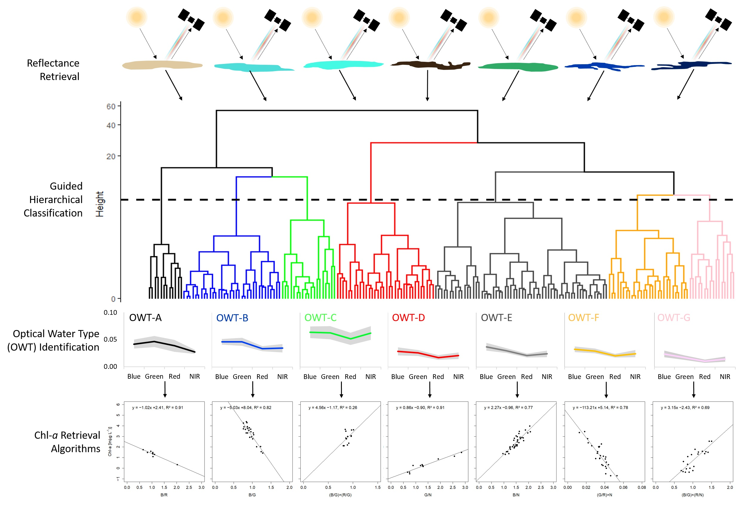
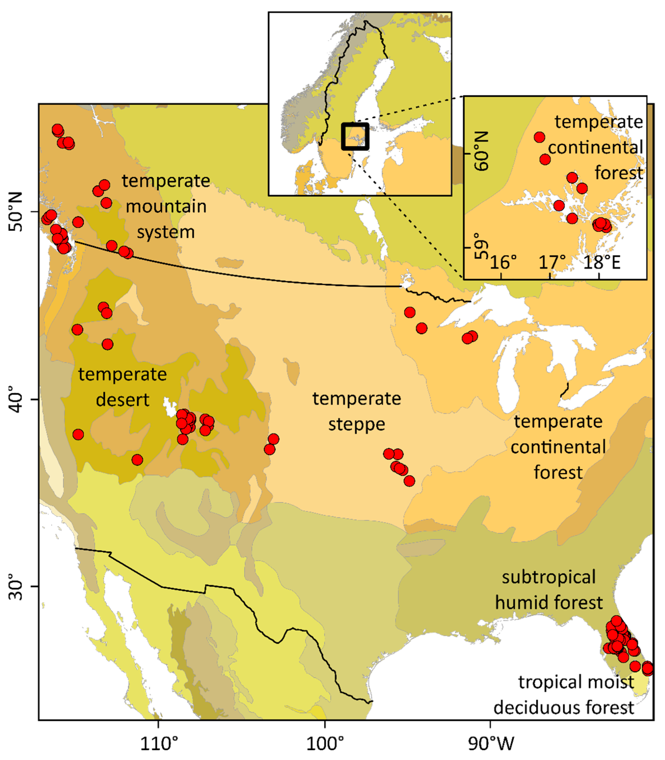
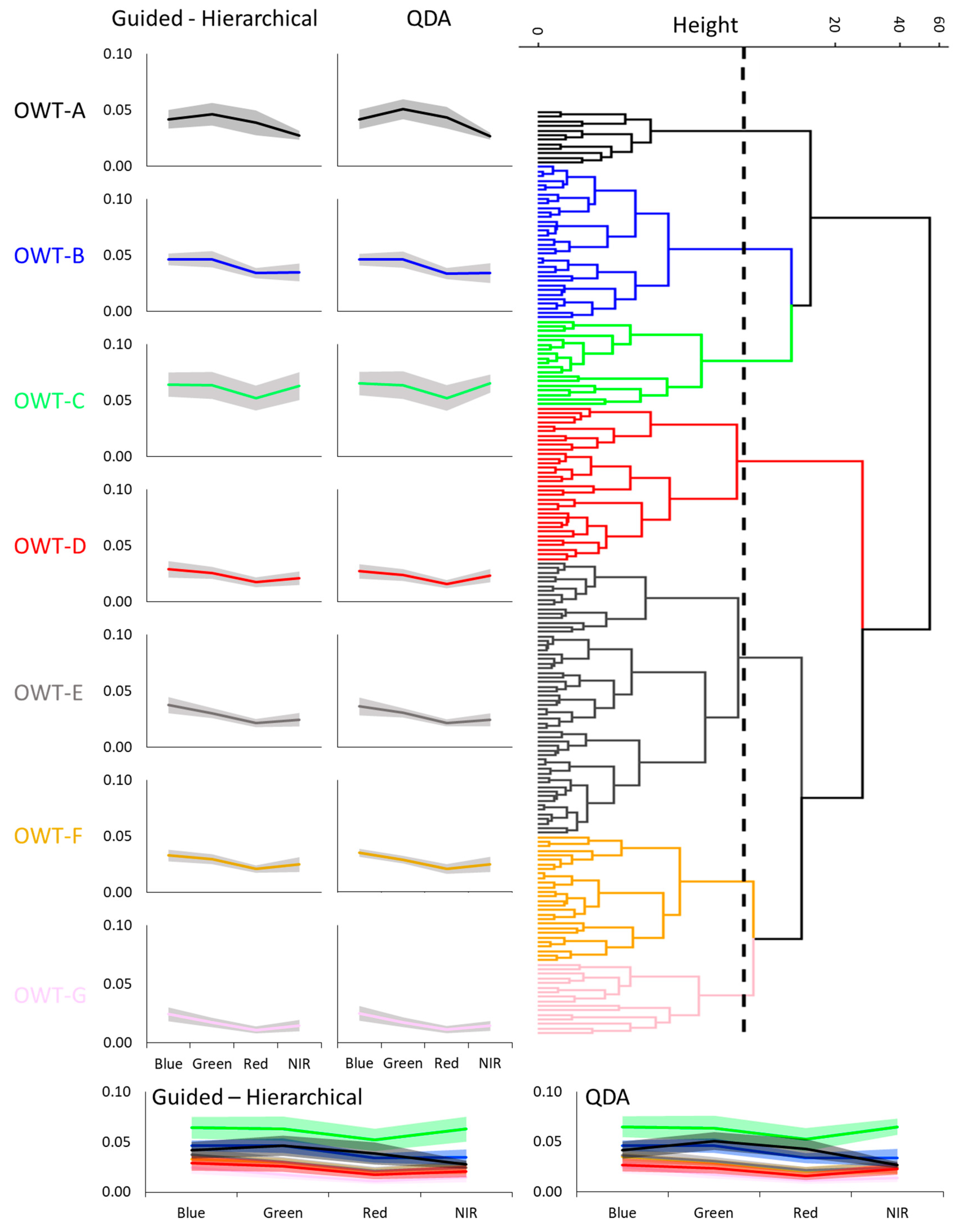
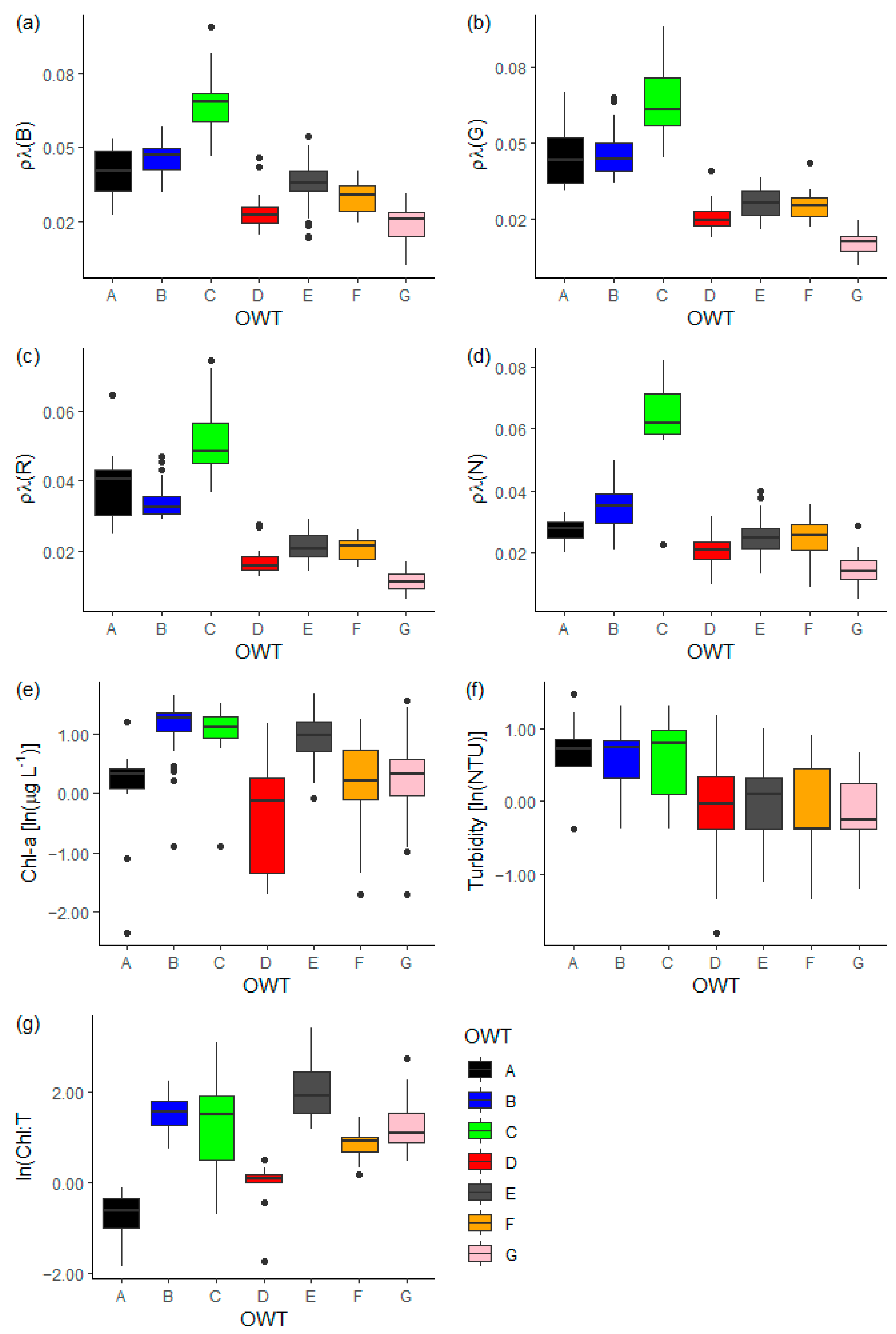
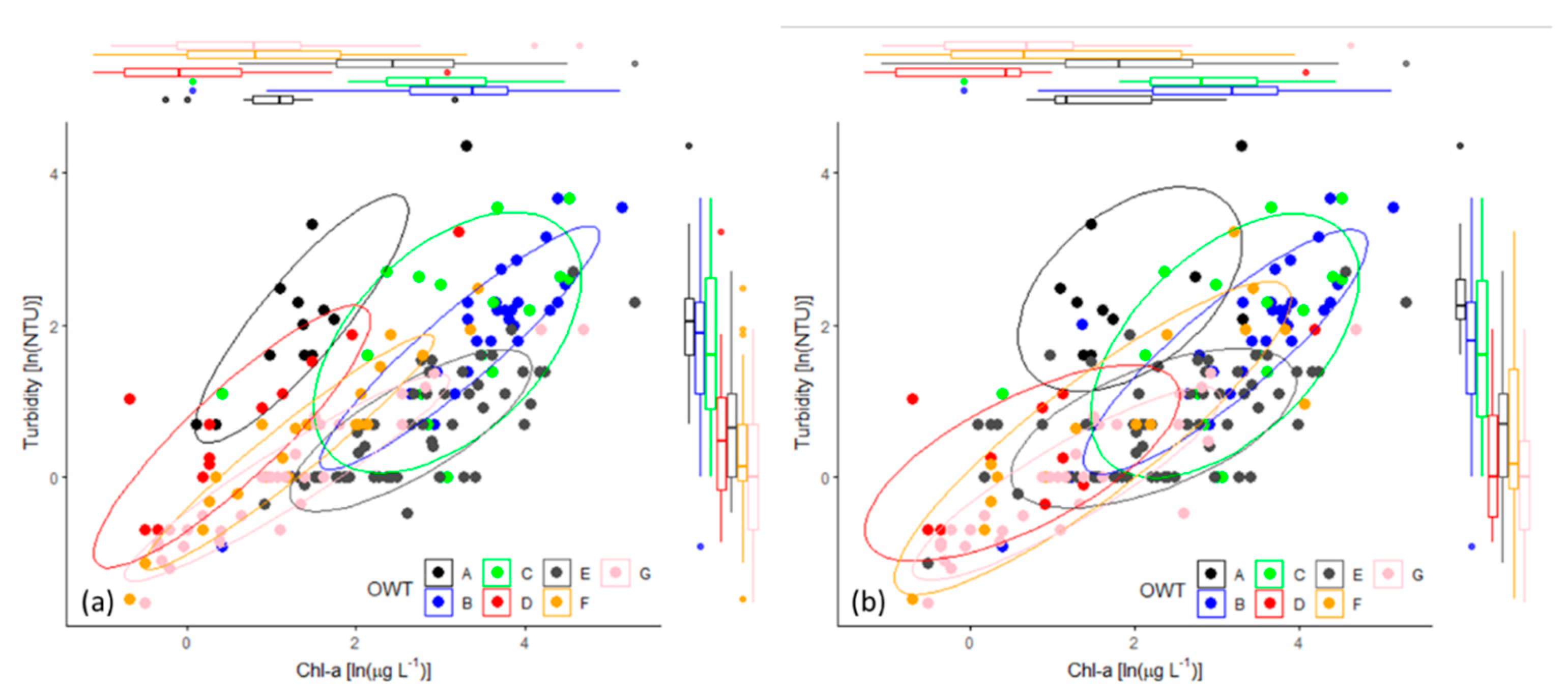
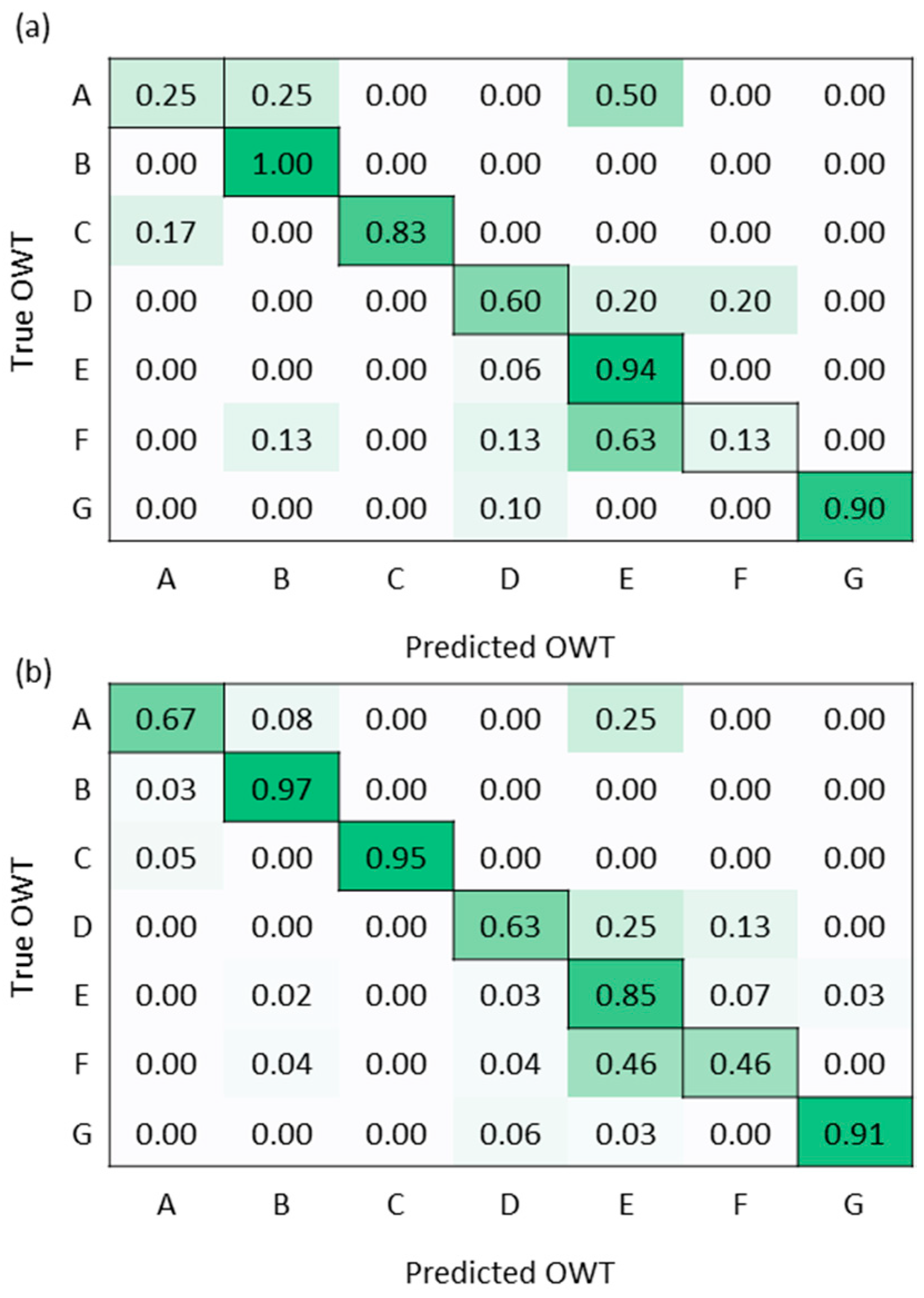
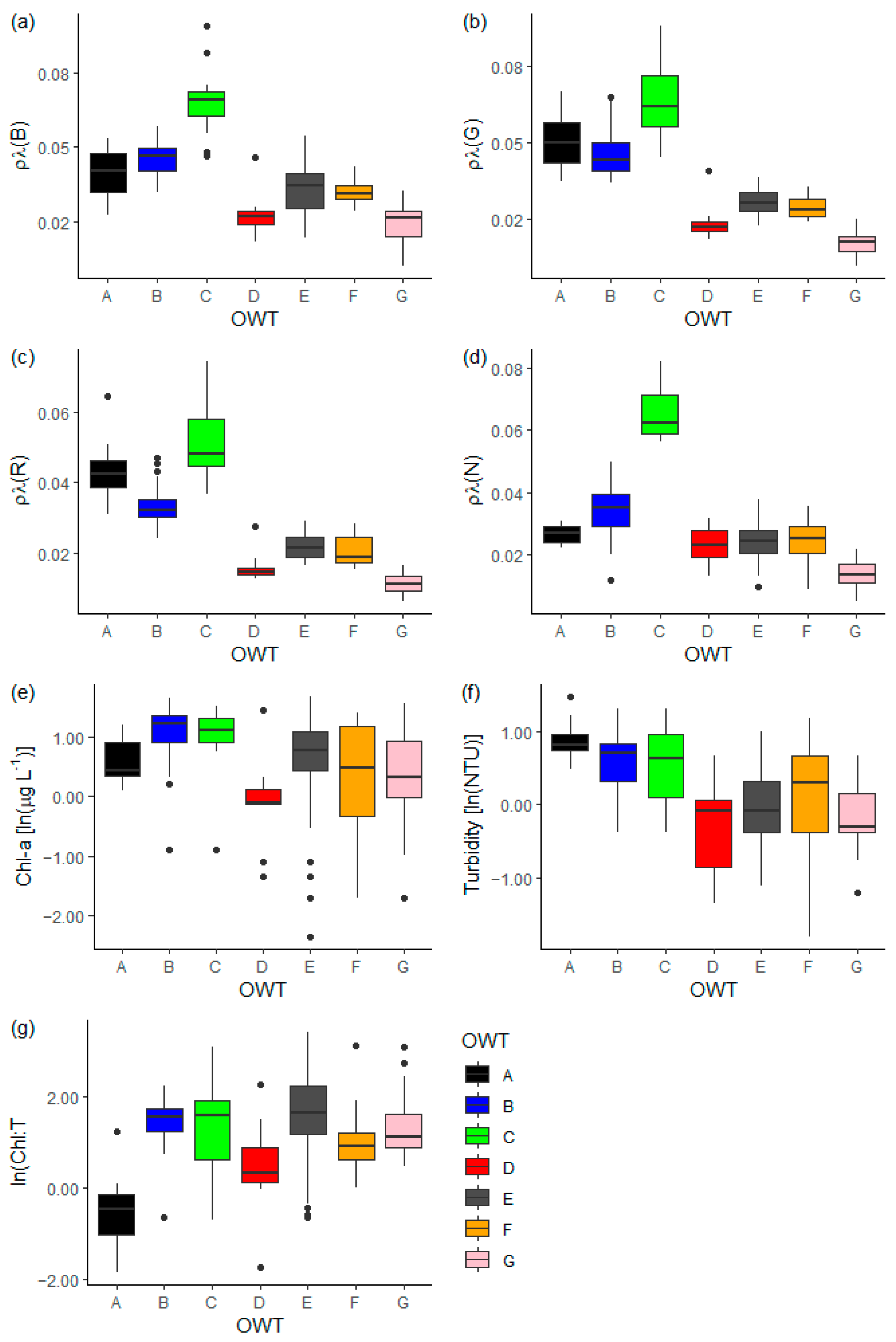
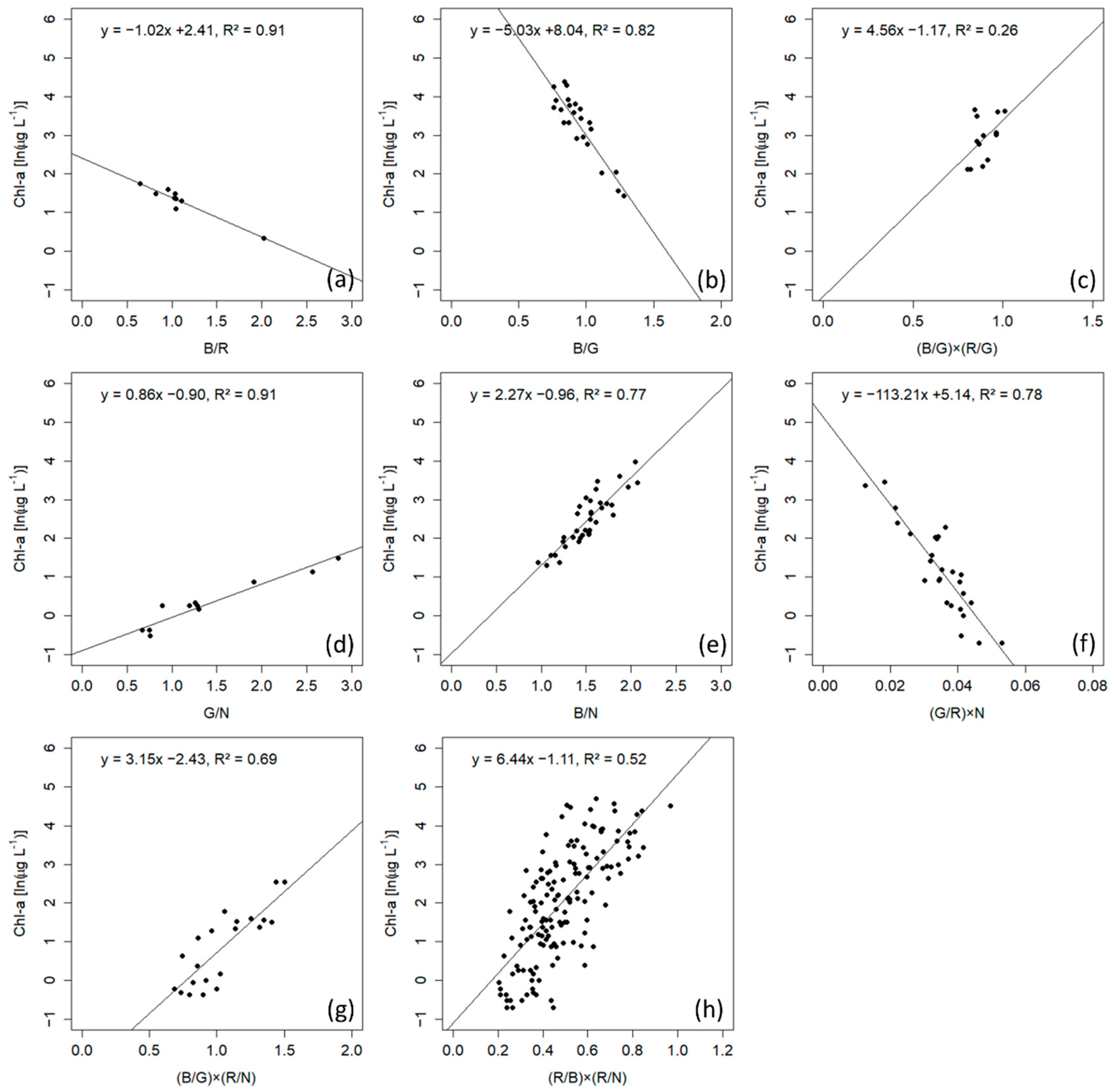
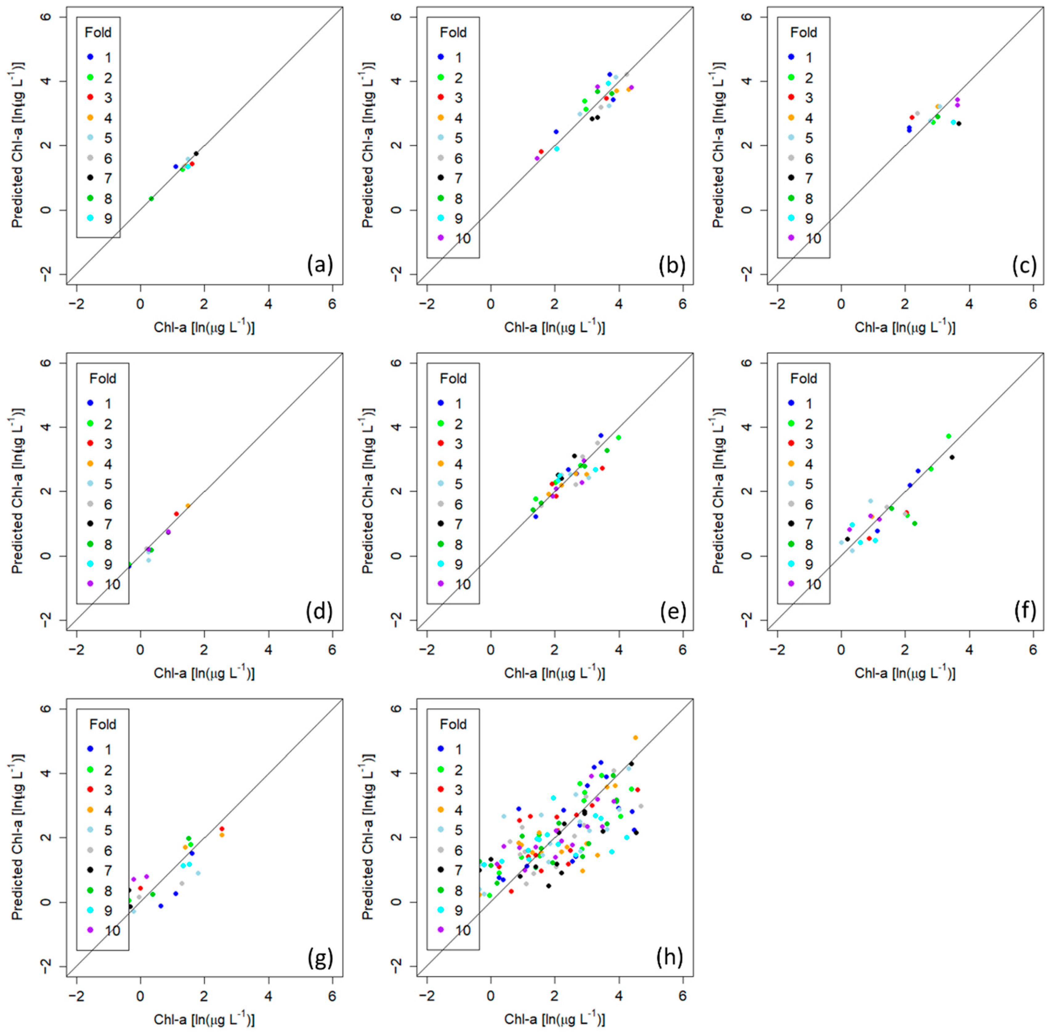
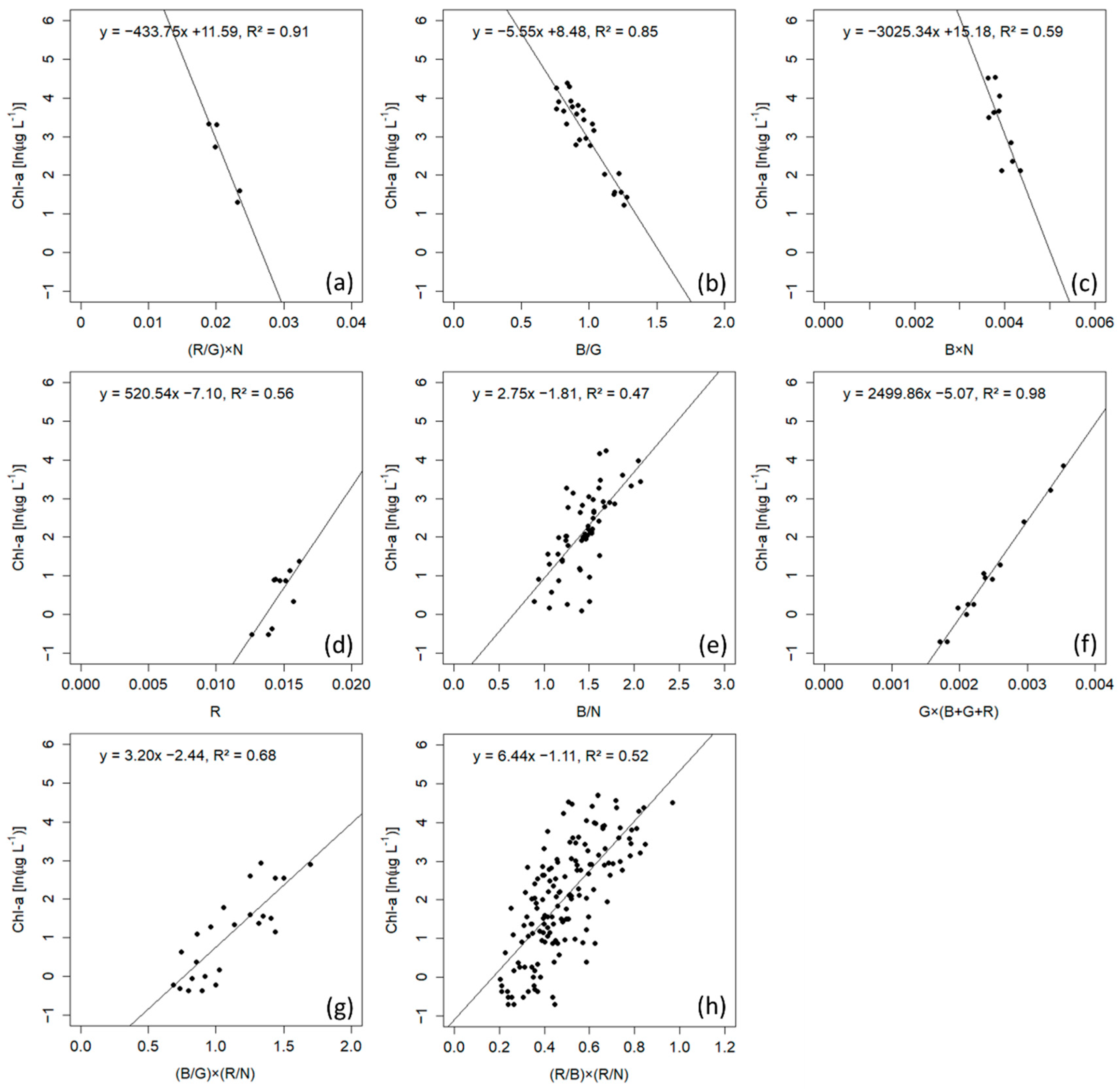
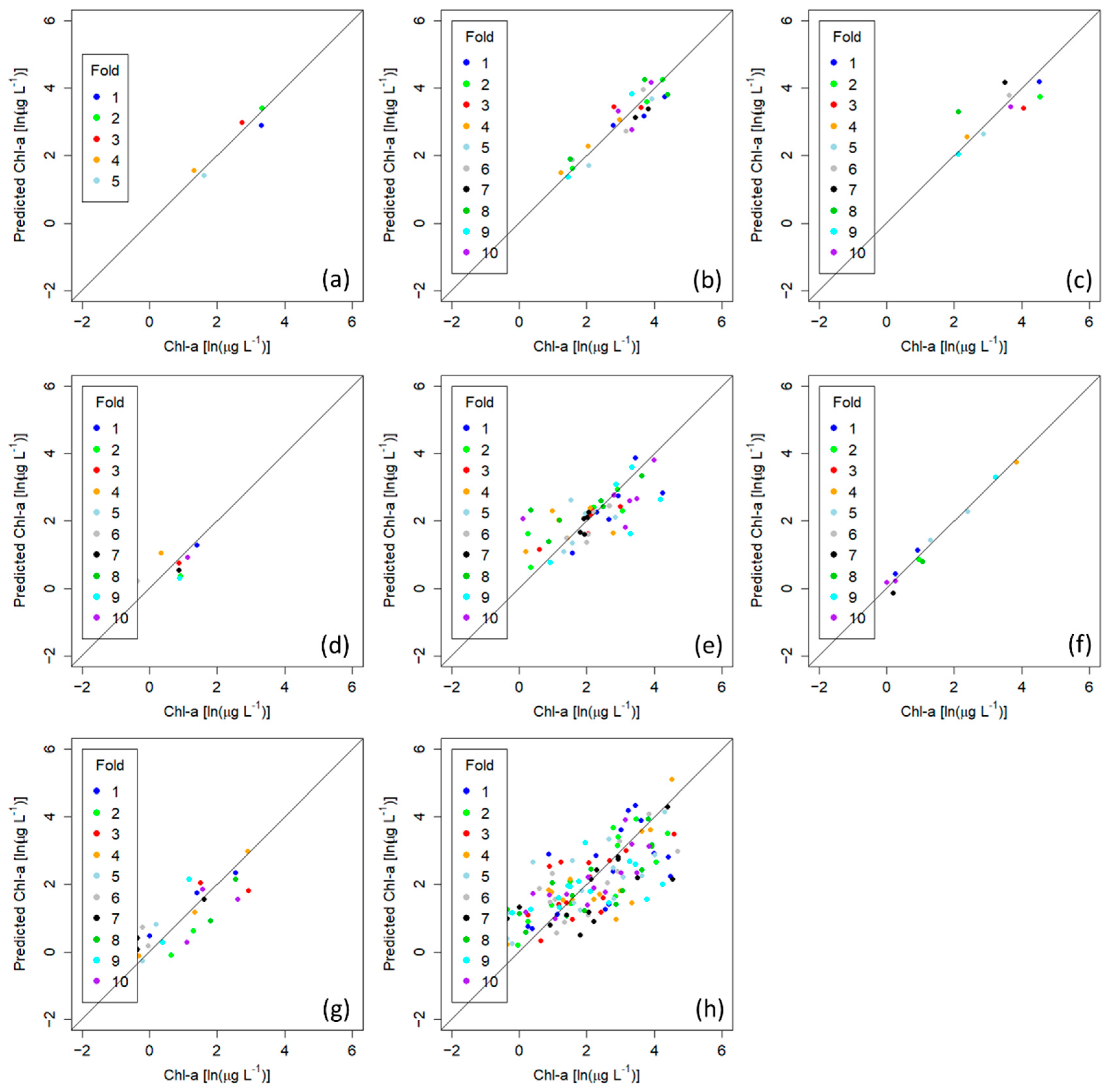
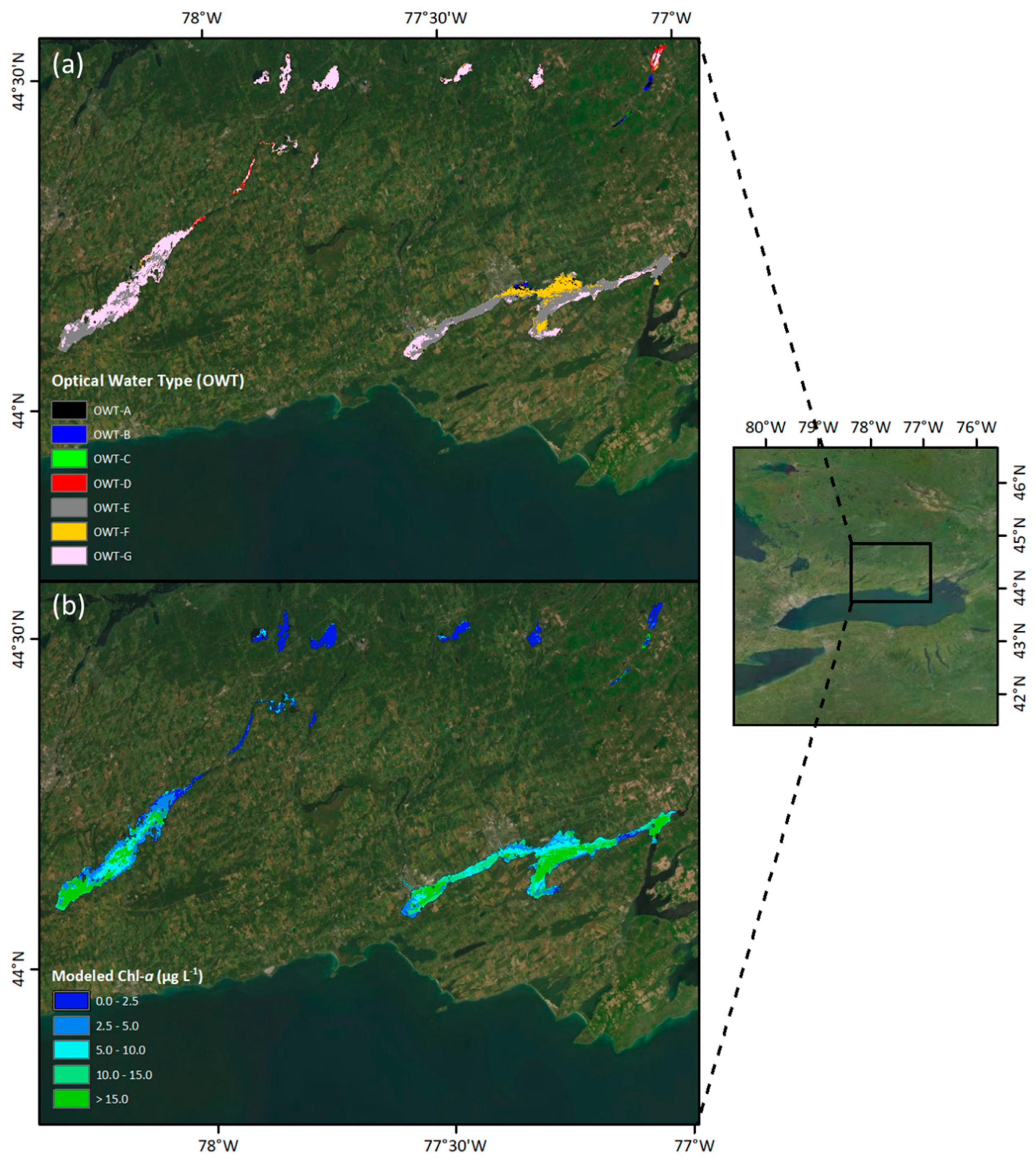
Table 1.
Summary statistics of ground-based chl-a and turbidity within each OWT for two different methods: unsupervised hierarchical clustering based on reflectance and water chemistry, and supervised quadratic discriminant analysis (QDA), trained using the hierarchical classes and the associated mean lake TOA reflectance (ρλ) per band (B = Blue, G = Green, R = Red, N = near infrared).
| Chl-a (μg L−1) | Turbidity (NTU) | Chl:T | Mean Lake ρλ | ||||||||||||
|---|---|---|---|---|---|---|---|---|---|---|---|---|---|---|---|
| OWT | Min | Med | Max | Min | Med | Max | Min | Med | Max | B | G | R | N | n | |
| Hierarchical Clustering | Ah | 1.1 | 4.0 | 27.2 | 2.0 | 7.8 | 78.0 | 0.2 | 0.5 | 0.9 | 0.042 | 0.046 | 0.039 | 0.027 | 12 |
| Bh | 1.5 | 33.6 | 171.0 | 0.4 | 6.7 | 39.0 | 2.1 | 4.8 | 9.3 | 0.046 | 0.046 | 0.034 | 0.035 | 34 | |
| Ch | 1.5 | 20.2 | 92.3 | 1.0 | 5.0 | 39.0 | 0.5 | 4.5 | 21.5 | 0.064 | 0.063 | 0.052 | 0.063 | 19 | |
| Dh | 0.5 | 1.3 | 24.9 | 0.4 | 1.7 | 25.0 | 0.2 | 1.1 | 1.7 | 0.029 | 0.026 | 0.017 | 0.021 | 16 | |
| Eh | 2.5 | 13.7 | 200.0 | 0.6 | 1.9 | 15.0 | 3.2 | 6.7 | 30.2 | 0.037 | 0.030 | 0.021 | 0.024 | 60 | |
| Fh | 0.5 | 3.0 | 31.4 | 0.2 | 1.2 | 12.0 | 1.2 | 2.5 | 4.2 | 0.033 | 0.030 | 0.021 | 0.025 | 28 | |
| Gh | 0.6 | 3.0 | 108.5 | 0.2 | 1.0 | 7.0 | 1.6 | 3.0 | 15.5 | 0.024 | 0.017 | 0.011 | 0.015 | 34 | |
| QDA | Aq | 3.0 | 4.7 | 27.7 | 5.0 | 9.5 | 78.0 | 0.2 | 0.6 | 3.5 | 0.042 | 0.051 | 0.043 | 0.027 | 10 |
| Bq | 1.5 | 29.3 | 171.0 | 0.4 | 6.0 | 39.0 | 0.5 | 4.8 | 9.3 | 0.046 | 0.046 | 0.034 | 0.034 | 36 | |
| Cq | 1.5 | 20.9 | 92.3 | 1.0 | 5.0 | 39.0 | 0.5 | 4.9 | 21.5 | 0.065 | 0.064 | 0.052 | 0.065 | 18 | |
| Dq | 0.5 | 2.4 | 66.0 | 0.4 | 1.0 | 7.0 | 0.2 | 1.4 | 9.4 | 0.027 | 0.024 | 0.016 | 0.023 | 15 | |
| Eq | 0.6 | 8.4 | 200.0 | 0.3 | 2.0 | 15.0 | 0.5 | 5.1 | 30.2 | 0.036 | 0.031 | 0.022 | 0.024 | 72 | |
| Fq | 0.5 | 2.9 | 58.7 | 0.2 | 1.2 | 25.0 | 1.0 | 2.5 | 22.6 | 0.035 | 0.029 | 0.021 | 0.025 | 19 | |
| Gq | 0.6 | 3.0 | 108.5 | 0.2 | 1.0 | 7.0 | 1.6 | 3.0 | 21.7 | 0.025 | 0.017 | 0.011 | 0.014 | 33 | |
Table 2.
Number of instances that each Landsat band (B, G, R, N) is present in one of the top ten performing (as indicated by r2) algorithms for chl-a retrieval per OWT. Chl:T + Ref refers to results of the unsupervised hierarchical clustering classification and QDA refers to the supervised classification.
| OWT-Chl:T + Ref | B | G | R | N | OWT-QDA | B | G | R | N |
|---|---|---|---|---|---|---|---|---|---|
| Ah | 7 | 5 | 5 | 4 | Aq | 3 | 6 | 8 | 10 |
| Bh | 8 | 7 | 6 | 8 | Bq | 8 | 8 | 8 | 6 |
| Ch | 8 | 10 | 6 | 2 | Cq | 10 | 8 | 3 | 3 |
| Dh | 4 | 7 | 5 | 10 | Dq | 5 | 8 | 7 | 5 |
| Eh | 7 | 4 | 8 | 9 | Eq | 10 | 4 | 8 | 7 |
| Fh | 3 | 3 | 8 | 10 | Fq | 6 | 6 | 10 | 8 |
| Gh | 5 | 4 | 6 | 10 | Gq | 4 | 3 | 8 | 10 |
Table 3.
Chl-a retrieval algorithm results (after outlier removal) for each OWT and for all lakes (“global”) using both unsupervised hierarchical and supervised QDA clustering. r2—adjusted r2; root mean squared error—RMSE; normalized RMSE—NRMSE; p-value—p; Breusch–Pagan constant variance—CV; Shapiro–Wilks normality—NM; mean absolute error—MAE; median absolute percentage error—MAPE; and bias. Filled boxes indicate that assumptions of linear regressions have been met (p < 0.05; CV and NM ≥ 0.05); empty boxes indicate that the assumptions have not been met.
| OWT | Algorithm | r2 | Adj. r2 | p | CV | NM | n | RMSE (μg L−1) | RMSLE (μg L−1) | NRMSE | MAE (μg L−1) | MAPE (%) | Bias |
|---|---|---|---|---|---|---|---|---|---|---|---|---|---|
| OWT-Ah | (B/R) | 0.91 | 0.90 | ■ | ■ | ■ | 9 | NA | NA | NA | NA | 6.37% | −0.02 |
| OWT-Bh | (B/G) | 0.82 | 0.81 | ■ | ■ | ■ | 23 | 11.74 | 0.31 | 0.55 | 10.16 | 9.41% | −2.27 |
| OWT-Ch | (B/G) × (R/G) | 0.26 | 0.19 | □ | ■ | ■ | 13 | 8.43 | 0.41 | 0.73 | 8.33 | 15.02% | −2.54 |
| OWT-Dh | (G/N) | 0.91 | 0.91 | ■ | ■ | ■ | 13 | 0.24 | 0.08 | 0.21 | 0.23 | 33.28% | 0.04 |
| OWT-Eh | (B/N) | 0.77 | 0.77 | ■ | ■ | ■ | 36 | 5.83 | 0.29 | 0.54 | 4.27 | 11.21% | −0.63 |
| OWT-Fh | (G/R) × N | 0.78 | 0.77 | ■ | ■ | ■ | 27 | 3.00 | 0.38 | 0.38 | 2.27 | 39.89% | −0.51 |
| OWT-Gh | (B/G) × (R/N) | 0.69 | 0.68 | ■ | ■ | ■ | 21 | 1.61 | 0.33 | 0.46 | 1.35 | 109.99% | −0.26 |
| OWT-Aq | (R/G) × N | 0.91 | 0.87 | ■ | ■ | ■ | 5 | NA | NA | NA | NA | 11.10% | −0.39 |
| OWT-Bq | (B/G) | 0.85 | 0.84 | ■ | ■ | ■ | 26 | 11.83 | 0.34 | 0.53 | 10.07 | 11.72% | −1.55 |
| OWT-Cq | (B*N) | 0.59 | 0.54 | ■ | ■ | ■ | 10 | 17.45 | 0.43 | 0.55 | 17.45 | 14.45% | −5.39 |
| OWT-Dq | R | 0.56 | 0.50 | ■ | ■ | ■ | 10 | 0.66 | 0.23 | 0.57 | 0.66 | 70.61% | −0.15 |
| OWT-Eq | (B/N) | 0.47 | 0.46 | ■ | ■ | ■ | 56 | 8.93 | 0.58 | 0.61 | 6.40 | 21.44% | −2.75 |
| OWT-Fq | G × (B + G + R) | 0.98 | 0.98 | ■ | ■ | ■ | 13 | 0.88 | 0.10 | 0.07 | 0.87 | 33.60% | −0.29 |
| OWT-Gq | (B/G) × (R/N) | 0.68 | 0.67 | ■ | ■ | ■ | 24 | 2.84 | 0.43 | 0.51 | 2.40 | 103.92% | −1.16 |
| Global | (R/B) × (R/N) | 0.52 | 0.51 | ■ | ■ | ■ | 147 | 19.66 | 0.81 | 0.85 | 11.22 | 34.11% | −4.13 |
Publisher’s Note: MDPI stays neutral with regard to jurisdictional claims in published maps and institutional affiliations. |
© 2021 by the authors. Licensee MDPI, Basel, Switzerland. This article is an open access article distributed under the terms and conditions of the Creative Commons Attribution (CC BY) license (https://creativecommons.org/licenses/by/4.0/).
Share and Cite
MDPI and ACS Style
Dallosch, M.A.; Creed, I.F. Optimization of Landsat Chl-a Retrieval Algorithms in Freshwater Lakes through Classification of Optical Water Types. Remote Sens. 2021, 13, 4607. https://0-doi-org.brum.beds.ac.uk/10.3390/rs13224607
AMA Style
Dallosch MA, Creed IF. Optimization of Landsat Chl-a Retrieval Algorithms in Freshwater Lakes through Classification of Optical Water Types. Remote Sensing. 2021; 13(22):4607. https://0-doi-org.brum.beds.ac.uk/10.3390/rs13224607
Chicago/Turabian StyleDallosch, Michael A., and Irena F. Creed. 2021. "Optimization of Landsat Chl-a Retrieval Algorithms in Freshwater Lakes through Classification of Optical Water Types" Remote Sensing 13, no. 22: 4607. https://0-doi-org.brum.beds.ac.uk/10.3390/rs13224607
Note that from the first issue of 2016, this journal uses article numbers instead of page numbers. See further details here.