A Deep Learning-Based Framework for Automated Extraction of Building Footprint Polygons from Very High-Resolution Aerial Imagery

Abstract

Accurate building footprint polygons provide essential data for a wide range of urban applications. While deep learning models have been proposed to extract pixel-based building areas from remote sensing imagery, the direct vectorization of pixel-based building maps often leads to building footprint polygons with irregular shapes that are inconsistent with real building boundaries, making it difficult to use them in geospatial analysis. In this study, we proposed a novel deep learning-based framework for automated extraction of building footprint polygons (DLEBFP) from very high-resolution aerial imagery by combining deep learning models for different tasks. Our approach uses the U-Net, Cascade R-CNN, and Cascade CNN deep learning models to obtain building segmentation maps, building bounding boxes, and building corners, respectively, from very high-resolution remote sensing images. We used Delaunay triangulation to construct building footprint polygons based on the detected building corners with the constraints of building bounding boxes and building segmentation maps. Experiments on the Wuhan University building dataset and ISPRS Vaihingen dataset indicate that DLEBFP can perform well in extracting high-quality building footprint polygons. Compared with the other semantic segmentation models and the vector map generalization method, DLEBFP is able to achieve comparable mapping accuracies with semantic segmentation models on a pixel basis and generate building footprint polygons with concise edges and vertices with regular shapes that are close to the reference data. The promising performance indicates that our method has the potential to extract accurate building footprint polygons from remote sensing images for applications in geospatial analysis.

1. Introduction

Information on the spatial distribution and changes of buildings has a wide range of applications in urban studies, such as urban planning, disaster management, population estimation, and map updating [1,2]. Local bureaus of urban planning and natural resource management used to expend high levels of manpower and material resources to obtain an accurate raster (i.e., map features described by a matrix of pixels, where each pixel contains an associated value) and vector (i.e., map features delineated by discrete vertices where each vertex defines the coordinates of the spatial objects) data of buildings [3]. The spaceborne and airborne technology provides abundant remote sensing images that have become increasingly important for extracting building information [4]. In early studies, pixel mixture is one important factor that influences building extraction when only fine- to coarse-resolution satellite images were available. Nowadays, advanced remote sensing technology offers very high-resolution images at sub-meter spatial resolution, making them attractive to extract accurate building footprint polygons. In the very high-resolution images, the influence of mixed pixels is minor, and the scene complexity becomes a new challenge for building footprint extraction. Currently, many government departments and industrial companies adopt manual methods to delineate the vector data of building footprints from high-resolution remote sensing images so as to obtain the vector maps that meet the accuracy requirements of surveying and mapping. As manual annotation is time-consuming and requires expertise [5], there is a need to develop an efficient and robust scheme for automated extraction of building footprint polygons from remote sensing images.

Classifying high-resolution remote sensing images to obtain the raster data of buildings has been extensively studied for decades [6,7]. Traditional methods include discovering and designing handcrafted features, such as spectral features, texture features, morphological features, and boundary features, as empirical indicators to distinguish buildings from other land surface objects in remote sensing images [8,9]. These methods often use empirical thresholds for classifying building objects and have drawbacks, such as insufficient uses of spectrum or spatial information and a high sensitivity to the choice of parameters or thresholds [10,11]. Machine learning models can overcome the shortcomings of the empirical methods and have been successfully applied for classifying buildings in remote sensing images [12]. Machine learning models, such as support vector machine, random forests, and artificial neural networks, use computer algorithms to establish the nonlinear relationships between inputs and targets through the training and learning processes based on many known samples. Machine learning methods have a high degree of automation and can efficiently reduce the confusion between buildings and other man-made features, but the input features to the machine learning models are often manually designed, such as low-level features or enhanced semantic features [13,14]. In recent years, with the development of computer technology, deep learning methods can automatically extract the features of different levels, such as low-level, middle-level, and high-level features from images [15], and have been widely used in the fields of computer vision and remote sensing image processing [16]. Earlier studies used patch-based convolutional neural networks (CNNs) to process image blocks to train and predict the class of the center pixel, but CNNs have difficulties in providing full-resolution classification maps [17,18]. Many studies on classifying buildings from remote sensing images now favor fully convolutional networks (FCNs), which implement an encoder–decoder framework and normally include convolution, down-sampling, and up-sampling layers for pixel-wise prediction or sematic segmentation [19,20]. For example, Maggiori et al. [21] utilized a fully convolutional architecture and designed a multiscale neuron module to produce dense predictions of building maps by alleviating the trade-off between recognition and localization. Ji et al. [22] proposed a Siamese U-Net that improves the classification performance of buildings, particularly large buildings. Huang et al. [23] designed an end-to-end trainable gated residual refinement network that has a competitive performance in extracting building raster data across urban and suburban scenes based on tests in a publicly available dataset. The above studies provide feasible methods for generating the classification maps of buildings using high-resolution remote sensing images. Some studies utilized the light detection and ranging (LiDAR) point cloud data to carry out building reconstruction given that the LiDAR data contain three-dimensional information related to buildings [24,25,26]. Gilani et al. [27] defined three general steps, including feature preservation, surface growing, and false plane elimination, to achieve automatic detection of building roof planes from the LiDAR point cloud. Although the LiDAR data can provide supplemental geometry features, the data acquisition of LiDAR is also more costly and complicated than those of optical sensors [28].

Extracting the vector data of building footprints from high-resolution remote sensing images is much more challenging than image classification. Traditional methods that directly extract the vector data of building footprints often manually design features or indexes that allow for generating the vector data of building footprints, but these methods are normally empirical and have difficulties for uses across images and scenes. Wang et al. [29] proposed a method to automatically extract rectangular buildings of different sizes and directions by combining image segmentation, scale-invariant feature transformation, and adaptive window Hough transform. Qin et al. [30] adopted straight line detection and graph loop searching to extract building boundaries with different shapes, sizes, and densities. Recently, some researchers have attempted using the deep learning methods to improve the extraction of building footprint polygons. Girard and Tarabalka [31] developed a deep learning-based model that could directly generate the vector maps, but the developed model has limitations in terms of extracting buildings with different shapes.

An indirect method that extracts building footprint polygons is to first classify buildings in remote sensing images, and then convert the raster format of buildings into a vector format. Buildings often have regular boundaries that consist of straight lines, while the pixel-wise semantic segmentation methods are often ineffective in describing the details of building footprint boundaries even if the produced classification map is highly accurate. It is, therefore, necessary to optimize the building footprint boundaries when converting them from raster data to vector data. One optimization approach is to improve the classification results of building boundaries in remote sensing images. Wu et al. [32] proposed a boundary-regulated network that consists of a modified U-Net and a multitasking framework to generate segmentation maps and building outlines by accounting for boundary regulation. To resolve the problem of blurry object boundaries, Marmanis et al. [33] proposed a DCNN models for semantic segmentation of high-resolution aerial images, which explicitly accounts for the boundaries of classes in the segmentation process. Taking the contours into consideration, Liao et al. [34] proposed a boundary-preserved building extraction approach. By embedding the contour information in the labels, the proposed approach can enhance the representation of building boundaries and improve the performance on boundaries of adjacent buildings. Another optimization approach is to improve the building boundary vertices when converting data formats. Some classic vector data processing algorithms, such as the Douglas–Peucker [35], Wang–Müller [36] and Zhou–Jones [37] algorithms, have been widely used by researchers. Maggiori et al. [38] proposed a new algorithm that uses a labeled triangular mesh to approximate the classification maps. Although many methods can improve the generated vector data of buildings, the obtained polygons generally do not match the building footprints well. One reason is that it is difficult to distinguish between adjacent buildings and deal with misclassified small patches during the map vectorization. Existing methods that extract building footprint polygons often have limitations; for example, they are only applicable for generating polygons of individual buildings with regular shapes such as rectangles.

Compared with pixel classification or segmentation, polygon extraction is a different and challenging task because it involves the transition of data representation. Specifically, pixel classification or segmentation of images transforms raster data into raster data, while the process that extract polygons from images transforms raster data into vector data. In the task of pixel-wise classification, the deep learning model only needs to discriminate the object pixels from the background pixels. In the task of polygon extraction, it needs to obtain at least the positions, the belongings, and the connections of the key vertices. Only a few studies have applied the deep learning models to detect the key points of geographical objects from remote sensing images. There are two main difficulties when using deep learning to directly detect a key point. First, compared to segmentation, the imbalance between positive and negative samples is severe. The annotated key points are much fewer than the background samples, and as a result, training and converging the deep learning network is difficult if we treat this task as a classification problem. Second, the number of key points that exist in an image is unknown. It is difficult to handle the outputs with irregular length using a convolutional neural network directly. Song et al. [39] proposed an FCN-based approach to detect building corners in aerial images. The corners are extracted by the contours of the predicted building footprints, which means that the performance of the corner detector largely relies on the accuracy of semantic segmentation. A deep learning-based model that treats the geolocation of building corners as direct objectives of optimization is not yet available.

One main problem is that existing segmentation-based methods extract building footprints with irregular outlines and blurred boundaries, which results in vectorized polygons with irregular shapes and redundant vertices. Given that existing deep learning-based studies mainly focus on improving the map classification or semantic segmentation of buildings, we aim to explore the ability of deep learning methods to learn and extract the vector data of buildings. The goal of this study is to develop a framework that synthesizes deep learning models to extract building footprint polygons from the remote sensing images and allow for the direct production of building maps in a vector format. In the developed framework, we use three deep learning models to perform different image processing tasks, including semantic segmentation, bounding box detection, and key point detection. A polygon construction strategy based on Delaunay triangulation was also designed to integrate these outputs effectively and thus generate high-quality building polygon data. The proposed framework is able to achieve comparable mapping accuracies with semantic segmentation models on a pixel basis and generate building footprint polygons with concise edges and vertices with regular shapes that are close to the reference data. Our method has the potential to extract accurate building footprint polygons from remote sensing images for applications in geospatial analysis.

2. Methodology

2.1. Overview

Our goal is to detect and generate the building footprint polygons that accurately describe the outline of individual buildings in a vector format from very high-resolution remote sensing images. Compared with the pixel-based raster data, the vector data contains not only the geometric information but also topological information, which provides another efficient way to represent real-world features in a geographic information system. Geometric information includes the positions of objects and their components in Euclidean space. Topological information includes the number, relationship, connection, and types of topological elements, such as vertices. Both geometric information and topological information are needed to represent objects correctly. To construct an individual building vector, we need both the accurate position of the vertices and the spatial relationship among vertices, which are able to generate polylines and polygons for the maps. The vector data use interconnected vertices to represent the object shapes, and each vertex describes its position using geographic coordinates in a spatial reference frame. As mentioned earlier, extracting building footprint polygons from aerial images involves tasks of different purposes, so it is difficult to optimize an individual deep learning network for different tasks. Hence, our approach is to split the main task of polygon extraction into several sub-tasks and utilize an appropriate deep learning model for each subtask. By integrating several methods in one framework, we are able to extract building footprint polygons from aerial images automatically and efficiently. As the vertices of building footprint polygons are often the corners of the building rooftop and the connections between building footprint corners are often straight lines, our strategy is to extract building polygons from remote sensing images by detecting the vertices of building footprint polygons first, and then finding the correct connections among them. Figure 1a illustrates the schematic workflow of the proposed building extraction method, which consists of four main steps: corner detection, semantic segmentation, object detection, and polygon construction. The framework takes very high-resolution aerial remote sensing images with RGB bands as inputs and extracts key information related to the building footprints from them. It adopts U-Net to produce the classification maps of buildings, Cascade R-CNN to detect building objects in the images, and Cascade CNN to detect building footprint corners. The features extracted using deep learning approaches from the remote sensing images are combined to produce building footprint polygons. The proposed deep learning-based framework for automated extraction of building footprint polygons (DLEBFP) is described in detail in the following sections.

2.2. Building Segmentation

U-Net, originally proposed for biomedical image processing and implemented in Caffe [40] was found to be effective in the semantic segmentation of remote sensing images [41,42]. U-Net used skip connections between the encoder and the decoder such that the decoder can receive low-level features containing abundant spatial and geometric information from the encoder, and thus it can generate precise classification maps. U-Net is widely used to extract various natural and man-made objects from remote sensing images. We use U-Net as a deep learning model for the semantic segmentation of the buildings. Figure 1b illustrates that U-Net utilizes the encoder–decoder architecture to make dense pixel-wise predictions. In the original implementation of U-Net, there are five convolutional blocks in the encoder and four upsampling blocks in the decoder. A convolutional block consists of two 3 × 3 unpadded convolutions, each followed by a rectified linear unit (ReLU). At the end of the block, a 2 × 2 max pooling operation with stride of 2 is appended for downsampling. After the process of each convolutional block, the number of feature channels doubled. In the decoder, the upsampling block consists of an upsampling operation of the feature map followed by a 2 × 2 convolution, which halves the number of channels. Two 3 × 3 convolutions followed by ReLU are used to process the concatenation of low-level features and features from the previous block. For the last layer in the decoder, a convolutional function followed by a sigmoid function is applied to map the output. In total, the U-Net has 23 convolutional layers, including 9 convolutional layers in the encoder and 14 in the decoder.

In this work, we modified the original U-Net. The modified U-Net shared similar architecture with original U-Net, and we added several modules to improve the performance of semantic segmentation. We adopted the encoder part based on ResNet34 [43] and used a residual unit consisting of multiple combinations of convolution layers, batch normalization (BN), and rectified linear unit (ReLU) activation. ResNet34 contains five convolutional blocks but more convolutional layers in each block, and the total number of convolutional layers was 34. Since many studies have suggested that a deeper network would produce more discriminative features and achieve better performance, the use of ResNet34 helps improve the segmentation results of UNet. Instead of directly passing through the convolution layers, the residual units utilize a shortcut connection and element-wise addition to transfer the input features directly to the output. It was found that the identity and projection shortcuts in ResNet could address the degradation problem during model training and also introduce neither extra parameter nor computation complexity [41]. The ReLU activation function is defined as $f\left(x\right)=\max \left(x,0\right)$ which reduces the possibility of vanishing gradient and accelerates the convergence of network during training [44,45]. BN performs the normalization for each training mini-batch and it allows for high learning rates and addresses internal covariate shift [46]. During the training stage, the mean and variance of features in a batch are first calculated and then used to normalize the features. In addition, two learnable parameters $\gamma$ and $\beta$ control the rescaling and shifting of the normalized values. As mini-batches are not used during inference, the moving average of the training set mean and variance are computed and used to normalize the features during the test procedure. For the decoder, compared to the blocks used in original U-Net, the BN layer is also inserted between the convolutional layer and the ReLU activation, such that we can accelerate the network convergence and improve the model performance. It should be noted that the cropping operation was removed from our network because the encoder used convolutional operation with the same padding rather than unpadded convolutions utilized in original U-Net.

Since the number of nonbuilding pixels is much higher than the number of the building pixels in most scenes, the effect of class imbalance could cause the learning process to be trapped in a local minimal of the loss function, making the classifiers strongly biased towards the background class [23,47]. To address the issue of class imbalance, we combined DiceLoss with binary cross-entropy loss as the objective function. The total loss calculation can be written as follows:

$$L_{seg}=L_{Dice}+L_{BCE}$$

(1)

$$L_{Dice}=1-\frac{2\times {{\displaystyle \sum }}_{i=1}^H{{\displaystyle \sum }}_{j=1}^W{y}_{ij}\times {\widehat{y}}_{ij}+\epsilon }{{{\displaystyle \sum }}_{i=1}^H{{\displaystyle \sum }}_{j=1}^W{y}_{ij} + {{\displaystyle \sum }}_{i=1}^H{{\displaystyle \sum }}_{j=1}^W{\widehat{y}}_{ij}+\epsilon }$$

(2)

$$L_{BCE}=-\frac{1}{H\times W}{\displaystyle \sum }_{i=1}^H{\displaystyle \sum }_{j=1}^W\left[y_{ij}\times \log {\widehat{y}}_{ij}+\left(1-y_{ij}\right)\times \log \left(1-{\widehat{y}}_{ij}\right)\right]$$

(3)

where $H$ is the height of the input image, $W$ is the width of the input image, $y_{ij}$ denotes the binary label of the pixel in the image (0 represents nonbuilding and 1 represents building), ${\widehat{y}}_{ij}$ represents the predicted probability of pixel ranging from 0 to 1, and $\mathit{\epsilon }$ denotes a factor used to smooth the loss and the gradient.

2.3. Building Object Localization

We use Cascade R-CNN to identify building objects from the remote sensing images. Note that many object detection models use intersection over union (IoU) to determine positive or negative samples; the use of a prescribed IoU significantly influences the model performance, because a low IoU easily leads to noisy detections and a higher IoU results in low detection accuracy because of model overfitting and sample mismatching. Cascade R-CNN can effectively address the abovementioned problems and improve object detection by adopting a multistage strategy for model training with an increasing IoU [48]. At the beginning of the model run, the results generated by the region proposal network are heavily tilted towards low quality, and thus the model uses a low IoU. Following the first stage of image classification and bounding box regression, the obtained bounding boxes are resampled using a higher IoU to provide samples with a higher quality. These processes go iteratively to improve the model performance for detecting objects from images.

Figure 1c illustrates the architecture of Cascade R-CNN model for building object detection. We use the feature pyramid network [49], which can detect multiscale objects by combining high-resolution low-level features and low-resolution high-level features to extract the feature maps at different scales. Lin, Dollar, Girshick, He, Hariharan, Belongie, and Ieee [49] demonstrated that using more than three stages in Cascade R-CNN would lead to a decreased performance. Thus, we chose the number of stages to be three and set the IoU thresholds of the detector in different stages as 0.5, 0.6, and 0.7, respectively. We used the same loss function in the feature pyramid network and the detection head, binary cross-entropy loss in the task of image classification, and smoothL1 loss in the task of bounding box regression:

$$L_{SmoothL1}=\{\begin{array}{c} 0.5\times {\left(y-\widehat{y}\right)}^2 if \left|y-\widehat{y}\right|<1\\ \left|y-\widehat{y}\right|-0.5 otherwise\end{array}$$

(4)

where $y$ denotes the reference values, and $\widehat{y}$ denotes the predicted values obtained from the models.

2.4. Corner Detection

Cascade CNN, initially proposed for multi-person pose estimation [50], is a key point detection network. We used Cascade CNN to detect building footprint corners. We removed the branch of part affinity field that was used to determine the overall relationship in the models because our network only focuses on predicting building footprint corners. Cascade CNN adopts a multistage strategy. In the first stage, the backbone network extracts high-level features from the input image, and convolutional layers with different kernel sizes are used to learn semantic information and produce a confidence map of the target key point. The model structure in the second stage is similar to that in the first stage, but the network concatenates the feature maps extracted by the backbone network and the confidence map generated from the previous stage as model inputs. The processes in the other stages are similar to those in the second stage.

Training a deep learning model to extract the geolocation of key points in an image is prone to model overfitting when directly using the coordinates as ground truth. We used heat maps as the ground truth for model developments, such that the network predicts the confidence map instead of the direct geographic coordinates of key points. The heat map is a two-dimensional map that represents the possibilities of the occurrence of the key points at each pixel. In a heat map, the pixel value of the possibilities ranges from 0 to 1. If one pixel is close to the annotated key point, the possibility value at the given pixel is close to 1. If multiple key points occur within one pixel, there is a peak corresponding to each key point. Using a heat map is advantageous, as it is possible to visualize the deep learning processes, given that the outputs can be multimodal [51]. We generate the heat map $S_k^{*}$ for each key point $k$ by placing a Gaussian function with fixed variance at the ground truth position of the building corners. The heat map $S_k^{*}$ at location $p$ is defined as follows:

$$S_k^{*}\left(p\right)=exp\left(-\frac{{\Vert p-x_k\Vert }_2^2}{2{\mathsf{\sigma }}^2}\right)$$

(5)

where $p$ denotes the pixel coordinate in the image, $x_k$ denotes the coordinate of the key point, ${\Vert p-x_k\Vert }_2^2$ is the squared Euclidean distance from the given pixel $p$ to the key point $x_k$, and $\mathsf{\sigma }$ is a constant that controls the spread of the peak.

As there could be many key points in a single image, a max operator is used to aggregate individual confidence maps of each corner and thus generate the complete confidence map used for training the models. The operator is defined as follows:

$$S^{*}\left(p\right) = \underset{k}{\max }{S}_k^{*}\left(p\right)$$

(6)

The architecture of Cascade CNN is shown in Figure 1d. We utilized VGG19 [52] as the backbone network in the model. The size of the feature map is one eighth of the size of the input image and the number of stages in Cascade CNN is 6. The loss function used in both the intermediate layers and the output layers is a mean square error (MSE) loss, which penalizes the squared pixel-wise differences between the predicted confidence map and the synthesized heat map. The loss function of the predicted confidence map is defined as follows:

$$L_{confmap}=\frac{1}{H\times W}{\displaystyle \sum }_{i=1}^H{\displaystyle \sum }_{j=1}^W{(y_{ij}-{\widehat{y}}_{ij})}^2$$

(7)

where H denotes the height of image, W denotes the width of the image, $y_{ij}$ is the value of the pixel (i, j) in the ground reference map, ranging from 0–1, and $\widehat{y}$ is the value of the pixel (i, j) in the predicted confidence map obtained from Cascade CNN.

Cascade CNN uses the inputs of the aerial images to generate confidence maps of key points. We extracted the locations of the building footprint corners by performing a nonmaximum suppression (NMS) on the heat maps [50,53]. Specifically, we used a max filter with the size of 3 × 3 slides along the heat map to extract the local maximum pixels as the pixels of key points. Note that we calculate the losses for the confidence maps in each stage during the training processes and avoid the problems of vanishing gradient or exploiting gradient when training the network.

2.5. Polygon Construction

To construct the structure of the building footprint polygons, we used two-dimensional Delaunay triangulation to transform the detected key points into the candidate polygons. Delaunay triangulation, as proposed by Boris Delaunay in 1934, has been widely used in computer graphics and geographical studies [54,55]. Given a set of discrete points, Delaunay triangulation generates a triangulated irregular network, where no points are located inside the circumcircle of any triangle in the network and the minimum angle of all triangles is the largest among all possible networks. We used the bounding boxes obtained by Cascade R-CNN to constrain the key points and constructed a triangulated irregular network for each individual building. Owing to the limitations in computational resources, there is a need to crop large remote sensing images, resulting in buildings being truncated at the borders of the cropped images. We defined the intersection points between the segmentation mask and the border of the cropped image as virtual corners (VC) and used them together with the key points detected by Cascade CNN for constructing a triangulated irregular network. The use of VC when constructing building polygons based on Delaunay triangulation could largely reduce erroneous triangles. For each triangle in the triangulated irregular networks generated by Delaunay triangulation, we calculated the ratio of the building areas obtained from the segmentation map generated using U-Net to the triangle areas and applied an individual threshold to classify the triangles as either building or nonbuilding triangles. All building triangles were merged to produce the building footprint polygons across the entire region.

3. Experiment Setup

3.1. Dataset

The performance of the deep learning model relies on a dataset with high-quality samples. An aerial imagery dataset from the Wuhan University (WHU) building dataset was used (http://gpcv.whu.edu.cn/data/ (accessed on 10 November 2020). This dataset consists of more than 84,000 independent buildings labeled in the vector format and the aerial images at a 0.075 m spatial resolution covering an area of 78 km² in Christchurch, New Zealand. This area contains buildings of various architectural types with varied colors, sizes, shapes and usages, making it ideal to evaluate the deep learning models. The original aerial images are open-source data provided by the Land Information New Zealand (LINZ) Data Service (https://data.linz.govt.nz/layer/53451-christchurch-0075m-urban-aerial-photos-2015-2016/ (accessed on 29 Aug 2021)). The photographs were taken around 2015 and 2016, and the images were ortho-rectified digital orthophoto maps (DOMs) with RGB channels in New Zealand Transverse Mercator (NZTM) map projection [22,56]. The spatial accuracy is 0.2 m with 90% confidence level. As shown in Figure 2, the area was divided into three sub-regions for model training, validation, and testing. The main reason for using the WHU dataset for model tests is that the vector data provided by the land information service of New Zealand have been carefully checked and corrected by cartography experts [22]. The high-quality vector data of building footprints can be easily transformed into raster building maps, bounding boxes, and heat maps with vertex coordinates for training and testing the deep learning models.

Additionally, we used the publicly available benchmark dataset, ISPRS Vaihingen semantic labeling dataset (https://www2.isprs.org/commissions/comm2/wg4/benchmark/2d-sem-label-vaihingen/ (accessed on 20 January 2021)), to test the robustness of the proposed framework. The Vaihingen dataset consists of pairs of images and labels at the spatial resolution of 9 cm. The dataset contains 33 true orthophotos with near infrared (NIR), red (R), and green (G) bands, which are beneficial for roof contour detection. These tiles have different image sizes with an average size of 2494 × 2064 pixels. The pixel-based labels have six categories, including impervious surfaces, buildings, low vegetation, trees, cars, and clutter. We manually delineated building footprint polygons based on both images and pixel-based labels for studies. We used six in the 33 tiles for testing and the others for model training and validation.

3.2. Implementation Details

All the deep learning models and experiments were implemented on the Ubuntu 18.04 system equipped with a single NVIDIA RTX 2080Ti GPU with 11 GB of memory under CUDA10.0 and cuDNN7.5. U-Net was implemented based on the open-source machine learning library of PyTorch (https://pytorch.org/ (accessed on 10 November 2020)). The encoder part in the network was initialized using a pretrained ResNet-34 model, and the network was trained with a batch size of four. We only used the feature maps that were generated from the first four stages to make predictions. An Adam optimizer was used to optimize the parameters with a learning rate of 0.0001. Data augmentation, including rotation, flipping, and random manipulation of brightness and contrast, was applied to the images at the training stage. The network was trained for 40 epochs using the training set, and the model that performed well in the validation set was stored. Cascade R-CNN was implemented using MMDetection, an object detection and instance segmentation code based on PyTorch. The backbone was initialized using a pretrained ResNeXt101 model. The basic module of the ResNeXt101 model was different from that of ResNet-34. It used a bottleneck design to decrease the parameters in the network and make it efficient. In ResNeXt101, group convolution was introduced to improve the model accuracy without increasing complexity. Feature maps obtained at all stages were used in the feature pyramid network to detect objects with different scales. The network was trained using the stochastic gradient descent optimizer with a batch size of four, an initial learning rate of 0.02, a momentum of 0.9, and a weight decay of 0.0001. We used the learning rate warmup with a ratio of 1/3 in the first 500 iterations. The total number of epochs was set to 100, and the learning rate was reduced to one-tenth of the current learning rate every 30 epochs. Cascade CNN was implemented based on PyTorch. When generating the heat maps, we set σ in the Gaussian function as 12. Data augmentation was also applied to the training data. The backbone was initialized using the pretrained VGG-19 model. Only the feature maps in the third stage were used for prediction. The entire network was trained using the stochastic gradient descent optimizer with a batch size of four, an initial learning rate of 0.02, a momentum of 0.9, and a weight decay of 0.0001. The network was trained for 50 epochs. All the model configurations and hyper-parameters were chosen according to parallel experiments.

Note that all model configurations and hyper-parameters were carefully designed according to parallel experiments. Hundreds of experiments were conducted to test the performances of possible configurations and hyper-parameters, and we chose the one that outperformed any other settings, namely the architecture and specific values presented above.

3.3. Comparative Methods

To understand the model performance, we compared DLEBFP with three different deep learning models for the semantic segmentation results in the raster format and with a popular approach for generating vector results on the WHU building dataset.

We applied the deep learning methods of U-Net, FCN, and SegNet [57] to produce semantic segmentation maps for model comparisons. FCN alters the original CNN structure to enable dense prediction. FCN uses transposed convolution to upsample feature maps to match the sizes of the images and exploit the skip layer strategy. FCN has proven its performance in terms of model accuracy and computational efficiency across several benchmark datasets. SegNet has an encoder–decoder architecture and is often used for evaluating the performance of semantic segmentation models. In SegNet, the pooling indices computed in the max-pooling step in the encoder are reused in the corresponding decoder to perform nonlinear upsampling. Normally, the memory required in SegNet is much less than FCN for the same task of semantic segmentation.

Additionally, we vectorized the semantic segmentation maps produced by U-Net and applied the Douglas–Peucker algorithm to generalize the vector maps. The Douglas–Peucker algorithm is widely used for processing vector graphics and cartographic generalization [35,58]. Many building extraction researches also chose the Douglas–Peucker algorithm for building vector simplification due to its simplicity and efficiency [59,60]. Additionally, its performance has been proven superior to other classic simplification algorithms, such as the Reumann–Witkam algorithm and the Visvalingam–Whyatt algorithm [58]. The Douglas–Peucker algorithm simplifies a curve that is composed of line segments to a similar curve with fewer points by accounting for the maximum distance between the original curve and the simplified curve. At each step, the Douglas–Peucker algorithm attempts to find a point that is the farthest from the line segment with the first and the last points as end points. If the distance between the farthest point and the line segment is smaller than a prescribed threshold, it decimates all points between the first and the last points; otherwise, it keeps the farthest point and recursively calls itself with the first point and the farthest point and then with the last point and the farthest point. The Douglas–Peucker algorithm can produce objective quality approximations [61]. We applied different thresholds for the maximum distance in the Douglas–Peucker algorithm (i.e., 0.1, 0.5, and 1.0 m) to produce building footprint polygons based on the classification maps derived from U-Net for five sub-regions and the entire study region. By comparing the results simplified by different thresholds, we are able to analyze the performance variance with thresholds. Moreover, the results of simplification by Douglas–Peucker are also used to compared with the vector generated by our methods DLEBFP to verify the superiority of our approach.

To test the robustness of the proposed method, we also conducted experiments in the ISPRS Vaihingen dataset and compared the comparative methods with DLEBFP. Similar to the experiments on the WHU dataset, we trained and analyzed the model performance on the Vaihingen dataset.

3.4. Ablation Studies

Ablation studies aim on investigating how individual or combination of features affect the model performance by gradually removing some features of the model. Ablation studies have been widely adopted in the field of remote sensing and computer science [62,63,64]. Here, we conduct experiments to investigate the ablated features of both the virtual corner and bounding boxes. In DLEBFP, virtual corners generated from the semantic segmentation maps and bounding boxes detected by Cascade R-CNN are both used to improve the model performance in producing the building vector data. We can still extract the building footprint polygons by methods without these components.

To evaluate the uses of virtual corners and bounding boxes, we set four kinds of experiments on the WHU dataset in the ablation studies, including a baseline method. The baseline method (hereinafter referred to as Baseline) only uses two deep learning models (i.e., Cascade CNN and U-Net) for feature extraction and Delaunay triangulation for polygon construction. In Baseline, we constructed the triangulation network based on the building corners detected by Cascade CNN and classified the constructed triangles into building or nonbuilding triangles based on the segmentation map extracted by U-Net. We merged all building triangles to produce building footprint polygons. In the other three experiments, we tested the virtual corners and bounding boxes detected by Cascade R-CNN and extracted the building footprint polygons by (1) the baseline method with bounding boxes (hereinafter referred to as Baseline + BB), (2) the baseline method with virtual corners (hereinafter referred to as Baseline + VC), and (3) the baseline method with both bounding boxes and virtual corners (hereinafter referred to as Baseline + BB + VC).

3.5. Evaluation Metrics

We evaluated the model performance based on the raster format and used the metrics, including precision, recall, and IoU, which have been widely used in the assessment of building extraction results [65,66]. For the raster map, precision is the ratio of the true positive pixels to all detected building pixels, recall is the ratio of the true positive pixels to the reference building pixels, and IoU is the ratio of the true positive pixels to the total number of true positive, false positive, and false negative pixels. IoU is extensively used in evaluating model performance for image classification, as it provides a measure that penalizes false positive pixels. The abovementioned metrics are defined as follows:

$$\text{Precision}=\frac{\text{TP}}{\text{TP}+\text{FP}}$$

(8)

$$\mathrm{Recall}=\frac{\mathrm{TP}}{\mathrm{TP}+\mathrm{FN}}$$

(9)

$$\text{IoU}=\frac{\text{TP}}{\text{TP}+\text{FP}+\text{FN}}$$

(10)

where true positive (TP) denotes the number of building pixels correctly classified as buildings, false positive (FP) denotes the number of nonbuilding pixels misclassified as buildings, and false negative (FN) denotes the number of building pixels that are not detected.

In addition to assessments based on the pixel-wise metrics, we computed the vertex-based F1-score (VertexF) as proposed by Chen, Wang, Waslander, and Liu [60] to evaluate the performance of the generated building footprint polygons. To derive VertexF, the extracted polygons and the reference polygons were interpreted as two different sets of vertices. We set a buffer distance for every ground truth vertex and then classified all the vertices of the extracted building polygon as true positive (TP), false positive (FP), and false negative (FN). VertexF is calculated as:

$${\mathrm{VertexF}}_{\mathrm{s}}=\frac{2{\mathrm{TP}}_{\mathrm{s}}}{2{\mathrm{TP}}_{\mathrm{s}}+{ \mathrm{FN}}_{\mathrm{s}}+{ \mathrm{FP}}_{\mathrm{s}}}$$

(11)

where the subscript $\mathrm{s}$ denotes the buffer distance, ${\mathrm{TP}}_{\mathrm{s}}$ is the number of true positive vertices, ${\mathrm{FN}}_{\mathrm{s}}$ is number of false negative vertices, and ${\mathrm{FP}}_{\mathrm{s}}$ is the number of false positive vertices. We tested the buffer distances at 0.5 m and 1.0 m, respectively.

Evaluating the mapping accuracies of vertices is particularly meaningful for the vector data, because a simple and accurate representation is crucial to the map production. Moreover, the mapping accuracies of vertices better reflect the required manual editing workload when converting the extraction results to real map products [60].

4. Results

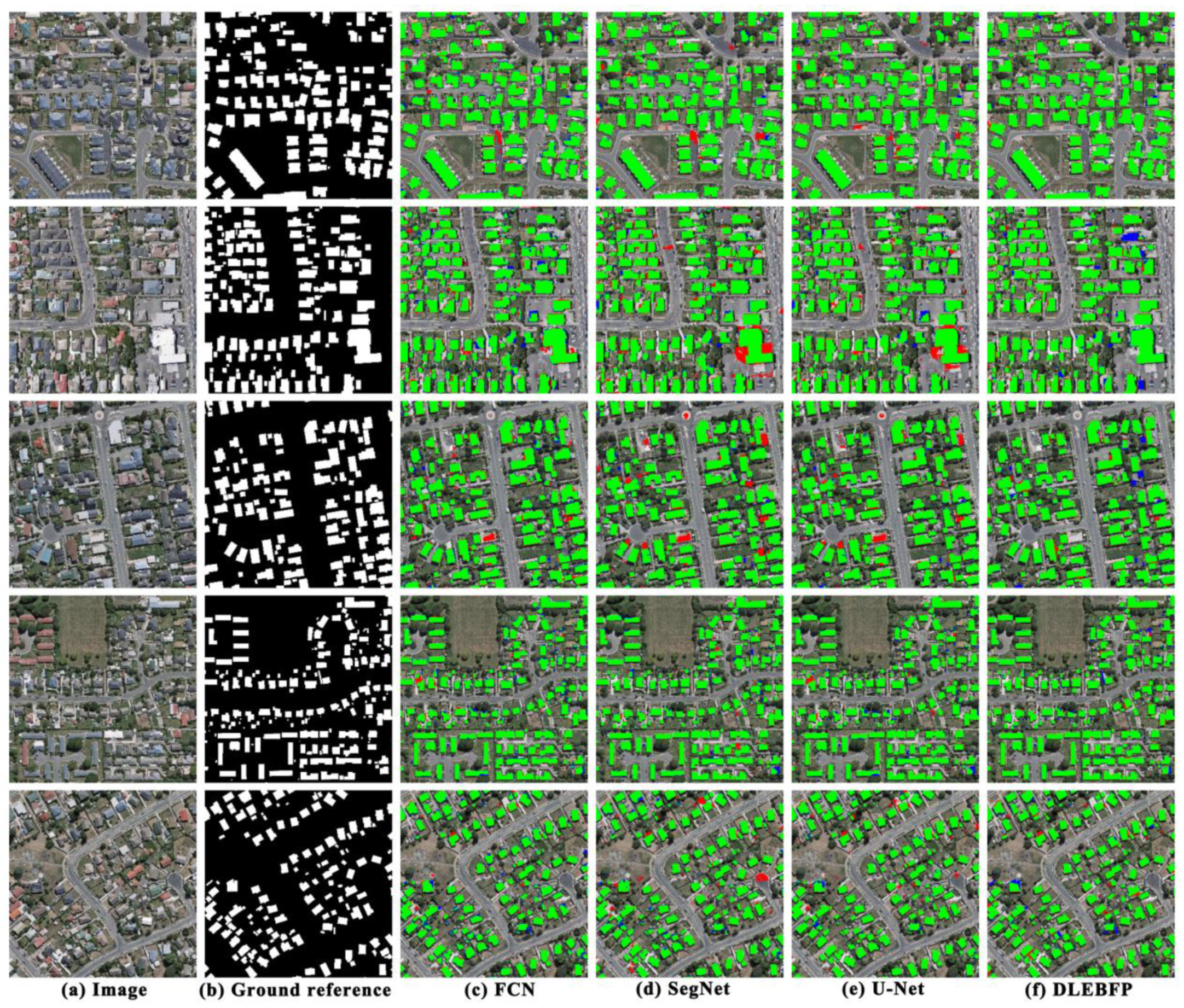
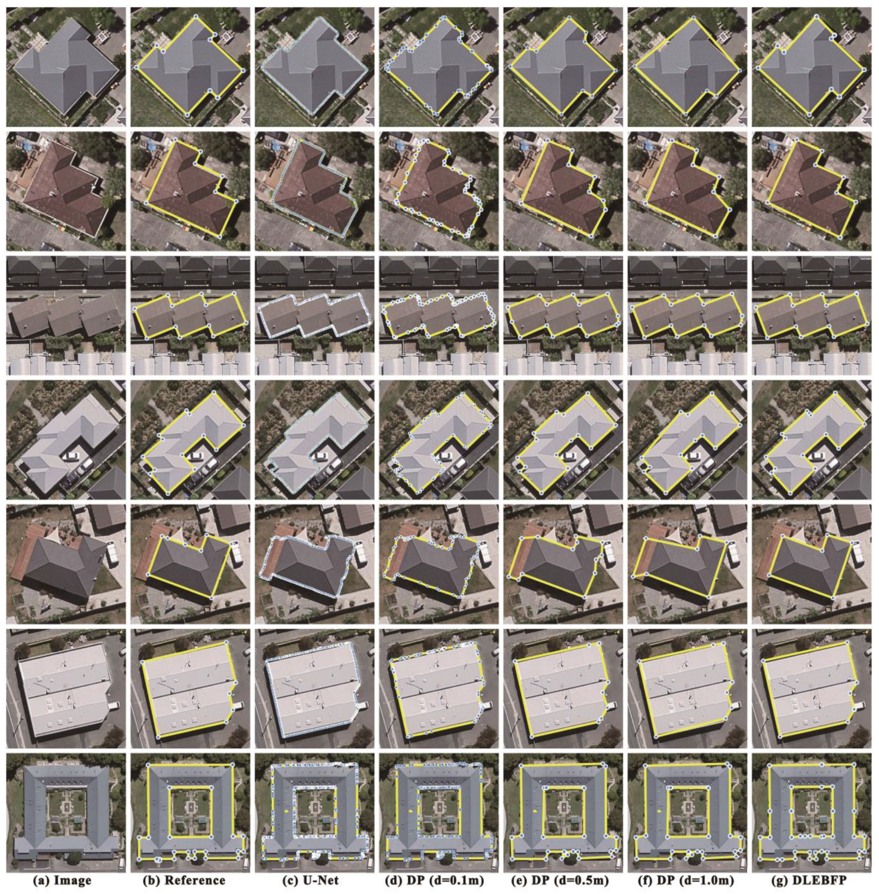
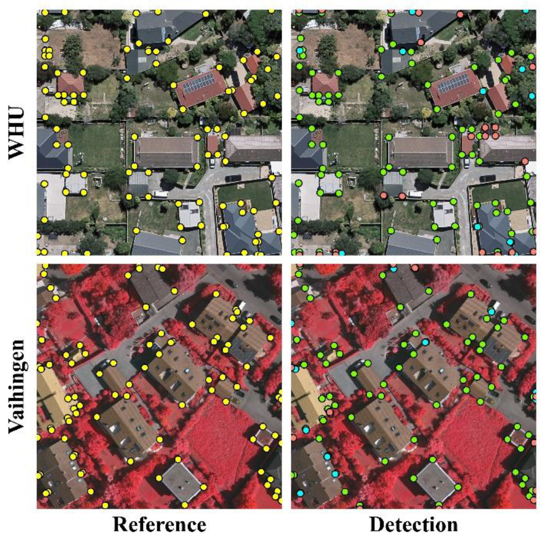
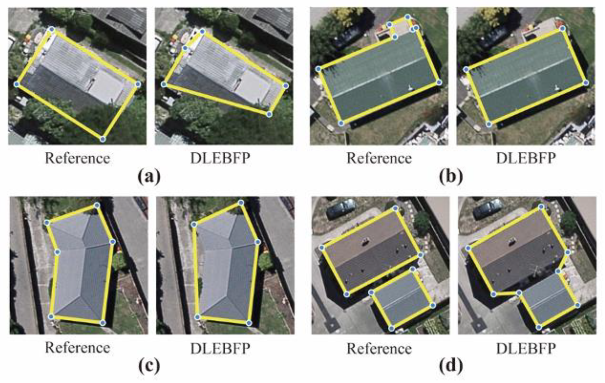
4.1. Results on WHU Dataset

Figure 3 shows the rasterized results of the extracted building footprints using different methods in the test area. Visually, the four methods have their own pros and cons. DLEBFP (Figure 3c) has fewer FPs than the three semantic segmentation models but contains more FNs. One reason is that the object detection method used in our approach is functionally similar to a filter that only screens pixels with high confidence of building footprints, such that it would improve the precision but impair the recall of the model. Among the three segmentation-based methods, FCN (Figure 3d) produces results similar to those of our method. FPs produced by FCN are less than those derived from either SegNet (Figure 3e) or U-Net (Figure 3f). Compared with the other methods, SegNet and U-Net generated more misclassified building pixels and generally performed well in extracting relatively large buildings. U-Net occasionally misclassified water pixels as buildings, for example, the pixels that are located in the river in the test area.

Figure 4 shows five scenes with the window size of 3000 × 3000 pixels, where the extent and location of buildings are marked in red rectangles in Figure 3a, for intuitive comparisons of the mapping results. All methods were able to identify most of the buildings correctly, demonstrating the power of deep learning approaches for the semantic segmentation of remote sensing images. Compared with the semantic segmentation models, our method generates fewer FPs. For example, in the first scene, three semantic–segmentation-based methods misclassified the road pixels as the building pixels (Figure 4c–e), and our method avoided misclassification because we used Cascade CNN to detect building footprint corners such that the falsely classified roads were screened out. In the second scene, many pixels surrounding a large building are also classified as buildings by both SegNet (Figure 4d) and U-Net (Figure 4e), whereas FCN (Figure 4c) produces a relatively lesser misclassification of pixels in the surroundings of the same building. In the same scene, our method distinguishes buildings from other objects and preserves the geometric details of building footprint boundaries. Although DLEBFP can extract most buildings accurately, there are some omission errors in buildings, resulting in higher FNs than the semantic segmentation methods. In general, among the three semantic segmentation methods, FCN did not extract the shape of buildings accurately and lost some details along the building boundaries, and U-Net and SegNet had similar performance across five scenes.

Table 1. The statistical results obtained by different models in the close-up scenes and the entire test dataset of the WHU dataset.

Model	Scene 1			Scene 2			Scene 3			Scene 4			Scene 5			Test Dataset
	Precision	Recall	IoU	Precision	Recall	IoU	Precision	Recall	IoU	Precision	Recall	IoU	Precision	Recall	IoU	Precision	Recall	IoU
FCN	0.941	0.941	0.889	0.925	0.921	0.857	0.918	0.942	0.868	0.942	0.917	0.868	0.938	0.909	0.858	0.932	0.897	0.841
SegNet	0.941	0.959	0.905	0.887	0.957	0.853	0.898	0.957	0.864	0.951	0.941	0.898	0.922	0.940	0.870	0.911	0.925	0.848
U-Net	0.945	0.970	0.917	0.908	0.956	0.872	0.907	0.964	0.879	0.947	0.949	0.902	0.933	0.954	0.893	0.917	0.933	0.861
DLEBFP	0.959	0.970	0.932	0.943	0.939	0.886	0.935	0.954	0.895	0.950	0.941	0.896	0.932	0.949	0.887	0.926	0.914	0.851

summarizes the quantitative evaluation results of our method and the three deep learning models in the close-up scenes and the entire testing dataset at the pixel level. The results of quantitative comparisons are in line with the visual examination results. Our method achieved the best results in Scene 1, Scene 2, and Scene 3, with the IoU values of 0.932, 0.886, and 0.895, respectively. U-Net achieves the best performance in Scene 4 and Scene 5 with the IoU values of 0.902 and 0.893, respectively, which are both 0.006 higher than our method. SegNet only performs better than our method in Scene 4, with an IoU of 0.898. FCN performs worse than the other methods across all scenes. For the entire testing data, DLEBFP outperforms FCN and SegNet and obtains a precision of 0.926, the recall of 0.914, and the IoU of 0.851. The IoU obtained by DLEBFP is lower than that obtained by U-Net. The high IoU of U-Net is due to more correctly classified building pixels, while the other methods omit these pixels, and thus U-Net has the highest recall values. DLEBFP has the highest precision values among all methods, because it combines the results of three deep learning models and effectively refines the building footprint detection on a step-by-step basis.

Figure 5 displays the vector maps of individual building examples obtained using different methods. Note that the building examples vary considerably in terms of colors, shapes, and surroundings. All methods are able to capture building footprint boundaries in general but with different accuracies. There are large differences among the methods in terms of the vertex number of the constructed polygons. As shown in Figure 5c, if we directly transform the semantic segmentation maps produced by U-Net into building footprint polygons without further processing, dense vertices are located near the building footprint boundaries, which are not useful for survey applications and not appropriate for data storage and transmission. Map simplification using the Douglas–Peucker algorithm with a 0.1 m threshold of the maximum distance (Figure 5d) results in fewer vertices than before, but many redundant vertices still exist when compared with the reference data. The number of vertices decreases as the threshold of the maximum distance in the Douglas–Peucker algorithm increases (Figure 5e,f), but the details of the building footprint boundaries are missing, resulting in inconsistency between the obtained building footprint polygons and the reference data in terms of building shapes. Our method (Figure 5g) performed the best among these methods in depicting the boundaries of buildings with different shapes and sizes. Note that the proposed method uses concise vertices to generate fine-grained building footprint boundaries and preserve geometric details as well as the shapes and structures of buildings. As seen from the second and seventh buildings, our method can accurately detect the buildings obstructed by trees. The multistage prediction in Cascade CNN can infer invisible building corners using the locations of the other corners and the extracted high-level features. In comparison, U-Net does not recover the buildings obstructed by trees and underperforms in comparison to our method in terms of the constructed building footprint polygons.

Table 2. Statistical results obtained using different models after vectorization on the WHU dataset.

Method	IoU Based on the Raster Data	IoU Based on the Vector Data	Changing Rate	Number of Reference Buildings	Number of Extracted Buildings	Number of Reference Vertices	Number of Extracted Vertices	VertexF0.5	VertexF1.0
DLEBFP	0.851	0.850	0.1%	15,675	14,687	134,246	135,623	0.668	0.744
U-Net	0.861	0.858	0.3%	15,675	18,302	134,246	7,990,152	0.022	0.025
U-Net + Douglas–Peucker (d = 0.1 m)	0.861	0.858	0.3%	15,675	18,302	134,246	1,138,969	0.114	0.134
U-Net + Douglas–Peucker (d = 0.5 m)	0.861	0.851	1.0%	15,675	18,302	134,246	278,541	0.229	0.309
U-Net + Douglas–Peucker (d = 1.0 m)	0.861	0.840	2.1%	15,675	18,302	134,246	250,132	0.216	0.295

lists the quantitative results obtained using different approaches. The vector results of U-Net have an IoU value of 0.858, which is slightly lower than that of the raster result. The results of our methods in the vector format have an IoU value of 0.850, which is lower than that of U-Net. In terms of the number of extracted buildings, the results of our method are closer to the reference data. DLEBFP generates 14,687 building footprint polygons, only 988 (approximately 6.3%) less than the reference data. One reason is that our method generates a few adjacent polygons that share building footprint corners with the other polygons, and the adjacent polygons could be recognized as a single polygon when conducting statistical analysis. The vector results of U-Net give 18,302 building polygons, 2627 (roughly 16.8%) more than the reference data, because there are many fragmented patches in the results. As mentioned earlier, the number of vertices is important for the management and application of the vector data. The vector results of U-Net have nearly eight million vertices, much higher than those of the ground reference. When generalizing the vector data using the Douglas–Peucker algorithm with the maximum distance thresholds of 0.1 m, 0.5 m, and 1.0 m, the number of vertices decreases to approximately 1 million, 278,541, and 250,132, respectively, and IoU decreases to 0.858, 0.851, and 0.840, respectively. Our method generates building footprint polygons with 135,623 vertices, only 1377 more than the reference data, and obtains an IoU value of 0.850. A vertex-based metric was calculated based on the extraction of different methods. As displayed in Table 2, our method outperforms other methods with VertexF_0.5 of 0.668 and VertexF_1.0 of 0.744, which are much higher than those derived from the other methods.

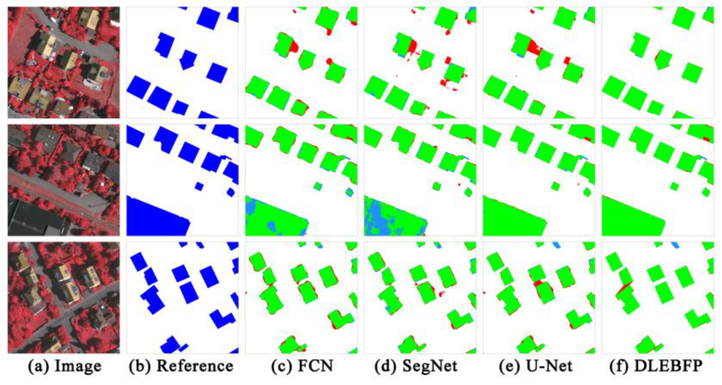
4.2. Results on Vaihingen Dataset

In order to test the robustness of the proposed method, we conduct extra experiments on the ISPRS Vaihingen dataset. Figure 6 displays the examples for the extraction results using different methods. Our method can obtain more accurate building footprints with distinctive boundaries and regular shapes. There are less FPs in the extraction results of our proposed method. For example, in the first and third images, there are many FPs located around the buildings in the results obtained using FCN, SegNet, and U-Net, and our method can discriminate it accurately. As shown in the second scene, both FCN and SegNet produce considerable FNs inside a large building, and both DLEBFP and U-Net can extract the large building accurately.

Table 3. Statistical results obtained by different models on ISPRS Vaihingen dataset.

Model	Precision	Recall	IoU	VertexF0.5	VertexF1.0
FCN	0.883	0.950	0.844	0.024	0.040
SegNet	0.910	0.932	0.854	0.023	0.030
U-Net	0.932	0.942	0.881	0.037	0.043
U-Net + DP0.1	0.932	0.941	0.879	0.198	0.245
U-Net + DP0.5	0.936	0.929	0.874	0.404	0.555
U-Net + DP1.0	0.938	0.917	0.865	0.417	0.562
DLEBFP	0.947	0.922	0.876	0.731	0.782

lists the statistical results for model comparisons on the ISPRS Vaihingen dataset. DLEBFP outperforms the other models in the metrics of precision, VertexF_0.5, and VertexF_1.0. Among all the tested methods, FCN produced the worst results with the IoU of 0.844. For the entire dataset, DLEBFP outperforms both FCN and SegNet and achieves a precision of 0.947, a recall of 0.922, and an IoU of 0.876. The IoU of DLEBFP is slightly lower than that of U-Net. The VertexF_1.0 of polygons obtained by three semantic segmentation models are less than 0.05, indicating that all these models are not directly suitable for practical applications, and further manual editing is required. We also compared the simplified results of U-Net with the results obtained by our proposed method. Simplification using the Douglas–Peucker algorithm with a 0.1 m threshold of maximum distance results in higher VertexF_0.5 and VertexF_1.0 than before, but the metric is still less than one third of that obtained by DLEBFP. As the threshold of maximum distance increases, the IoU of U-Net becomes lower than that of our method, but both Vertex-F_1.0 and Vertex-F_0.5 were still lower than that of DLEBFP. Taking both pixel-based and vertex-based evaluation results into consideration, DLEBFP can generate building footprint polygons better than the comparative methods. Overall, the performance of DLEBFP on the Vaihingen dataset are better than on the WHU dataset as indicated by both the pixel-based and vertex-based metrics, probably because the ISPRS Vaihingen datasets have high quality images and accurate image registrations.

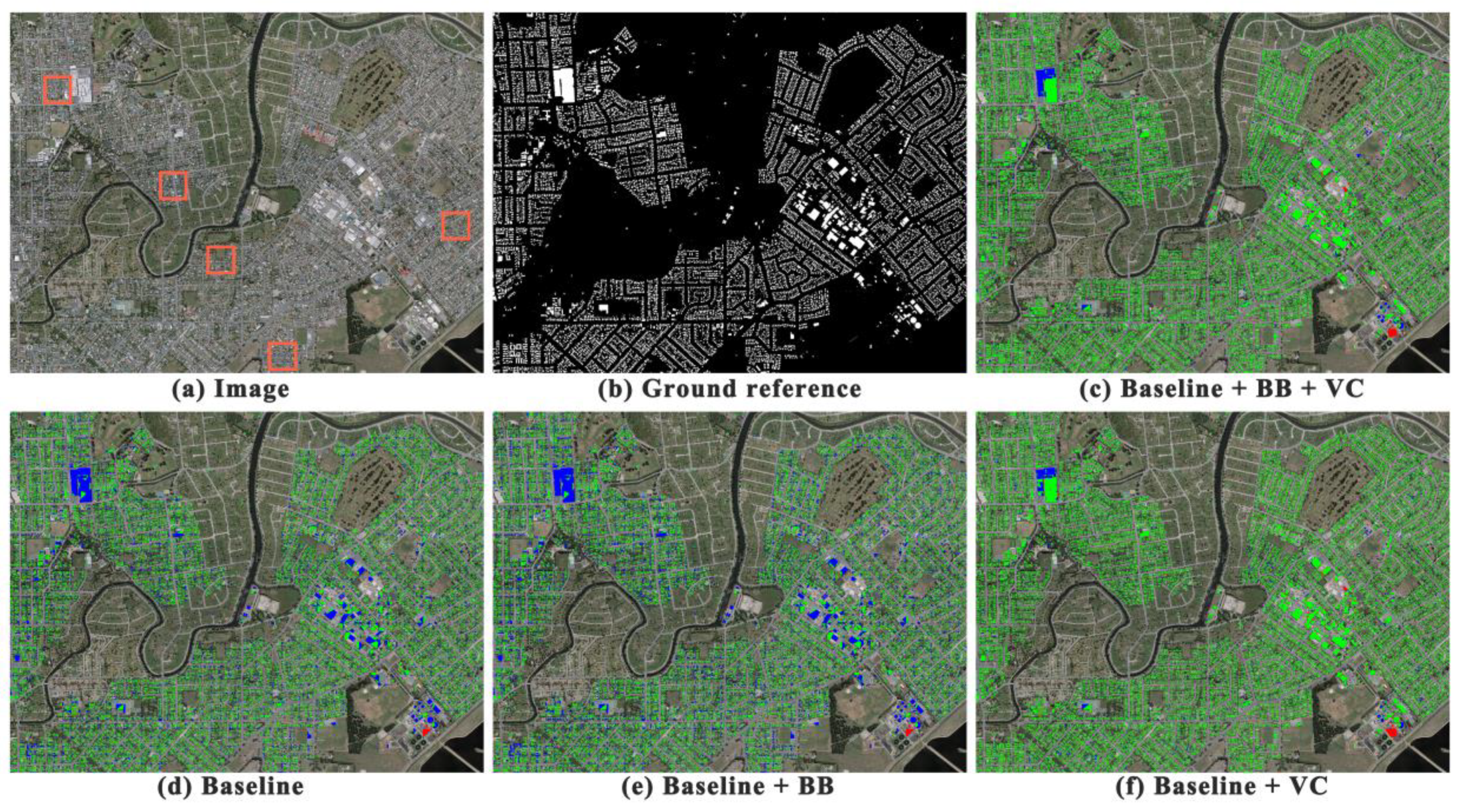
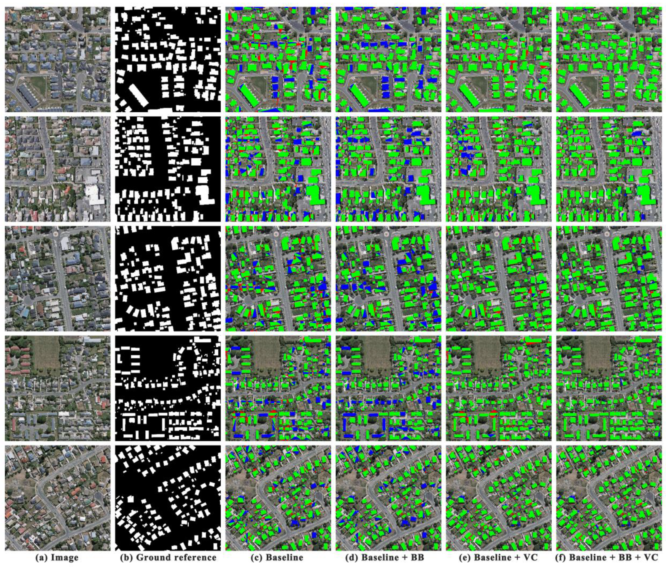
4.3. Ablation Studies

Figure 7 displays the results of the ablation experiments in the test area. The results of Baseline (Figure 7d) and Baseline + BB (Figure 7e) are similar, and both have considerable FNs and large omission errors in building detection. The extracted results using the Baseline + VC approach are generally comparable to those of Baseline + BB + VC. Visual comparisons suggest that both methods can extract most of the buildings correctly, but the Baseline + BB + VC method produces more FNs.

Figure 8 shows the results of the ablation experiments in the selected scenes of the test areas as marked in red rectangles in Figure 7a. As shown in Figure 8c, the Baseline method produces many FPs in the gaps among buildings and does not extract buildings accurately. Because the Delaunay triangulation generates triangles of buildings that share one or more corners with the other buildings, it could result in the adhesion of buildings. By applying the constraint of bounding boxes, the results of Baseline + BB (Figure 8d) show a reduced number of FPs among buildings but have many FNs because of missing buildings at the edge of the cropped images in the deep learning models. Baseline + VC (Figure 8e) achieves larger improvements over the Baseline method by reducing FNs considerably and detecting most of the erroneously mapped buildings correctly, but still results in considerable FPs among buildings. Baseline + BB + VC (Figure 8f), the complete method, integrates the advantages of the earlier two strategies and considerably reduces both FPs and FNs of buildings.

Table 4. Statistical results obtained in the ablation experiments.

Model	Scene 1			Scene 2			Scene 3			Scene 4			Scene 5			Test Dataset
	Precision	Recall	IoU	Precision	Recall	IoU	Precision	Recall	IoU	Precision	Recall	IoU	Precision	Recall	IoU	Precision	Recall	IoU
Baseline	0.885	0.776	0.705	0.891	0.771	0.704	0.875	0.792	0.712	0.869	0.702	0.635	0.906	0.817	0.753	0.882	0.736	0.670
Baseline + BB	0.958	0.737	0.714	0.943	0.743	0.711	0.926	0.736	0.694	0.941	0.653	0.627	0.927	0.790	0.743	0.918	0.706	0.664
Baseline + VC	0.914	0.954	0.877	0.911	0.890	0.820	0.909	0.954	0.871	0.896	0.931	0.840	0.925	0.946	0.879	0.905	0.911	0.832
Baseline + BB + VC	0.959	0.970	0.932	0.943	0.939	0.886	0.935	0.954	0.895	0.950	0.941	0.896	0.931	0.949	0.887	0.926	0.914	0.851

lists the quantitative results in the ablation experiments. For all five scenes, Baseline + BB could achieve a higher precision but a lower recall than Baseline. Compared with the Baseline method, the Baseline + BB method has a lower IoU in Scenes 3, 4, and 5, and a higher IoU in Scenes 1 and 2. Applying the constraint of bounding boxes did not enhance the model performance effectively. Compared with Baseline, the Baseline + VC method increases both recall and IoU and achieves the IoU values higher than 0.82 in five scenes, indicating that adding virtual corners helps reduce omission caused by image clipping. By integrating two improvement strategies, the Baseline + BB + VC method achieves the best performance in five different scenes. Compared with the Baseline + VC method, adding the constraints of bounding boxes could increase the values of precision, recall, and IoU. The impact is different from that when only adding the constraints of bounding boxes to Baseline, implying that the strategy of using bounding boxes only improves the model accuracy when buildings can be extracted more accurately. The performance of these methods is consistent in the entire test dataset with that on the five scenes. Compared with Baseline, Baseline + BB reduces IoU by 0.6% and Baseline + VC increases IoU by 16.2%. The Baseline + BB + VC method outperforms the other methods and achieves the best performance with a precision of 0.926, a recall of 0.914, and an IoU of 0.851. In comparison with Baseline, the precision, recall, and IoU of our method increased by 4.4%, 17.8%, and 18.1%, respectively.

5. Discussion

By combining the deep learning models for different tasks, our method can accurately extract building footprint polygons from very high-resolution aerial images. One advantage of our method is that it can extract building footprints with sharp boundaries in a vector format and use concise vertices to represent building footprint boundaries that are close to the ground reference. Another advantage of our method is that it can be executed on a regional scale instead of on an individual building. The reasons our method performs well are as follows. First, we used a deep learning model to detect the building footprint corners, which are used to guide the construction of building footprint polygons. Compared to the key point detection methods in the traditional methods, such as Harris and scale-invariant feature transform, the deep learning model can detect building footprint corners accurately. The traditional methods likely detect erroneous key points belonging to other man-made objects, such as roads. Second, our method integrates the multi-task results generated by the deep learning models based on the Delaunay triangulation. The ensemble framework enhances the model performance and makes it possible to automatically extract building footprint polygons from remote sensing images on a regional scale.

The accuracy of the corner detection influences the performance of the entire framework and Figure 9 exhibits the corner detection results on the two studied datasets. As shown in the figure, most of the corners can be detected by Cascade CNN despite of errors. First, our method cannot detect the corners that are severely obscured by trees. Although Cascade CNN can infer the existence of corners sheltered by trees in some cases, the predicted location of corners often deviates from their real locations. Second, a few redundant points that did not exist in the ground truth data were detected because these points have representation similar to building corners. The redundant detected points have limited impacts on the overall performance of our results because such points are normally removed when we classified the triangles based on the semantic segmentation maps. In addition, our method performs weakly on the corners that are closely located. It is difficult to accurately and completely distinguish adjacent corners. In this case, an incomplete set of corners causes a loss of geometric details and decreases the accuracy of the extracted building footprint polygons. When comparing with the results of corner detections on the WHU dataset, Cascade CNN performs better in the Vaihingen dataset. Visually, the results in the Vaihingen dataset have less omitted corners than in the WHU dataset. The statistical results associated with vertex-based evaluation metrics illustrate that the model performance in the Vaihingen dataset is better than in the WHU dataset. The differences in the model performance are likely due to different standards of classification labels and image quality. In the Vaihingen dataset, fewer buildings are obscured by trees or the other objects, and the sheltered buildings are not annotated as the building pixels. By comparison, the WHU dataset has more sheltered buildings that are still labeled as the building pixels in the ground truth maps. It is, therefore, challenging to detect building corners in the WHU dataset. DLEBFP achieves higher IoU in the Vaihingen dataset than in the WHU dataset because better corner detection results were obtained in the Vaihingen dataset when using Cascade CNN.

Our framework may extract inaccurate building footprint polygons and Figure 10 exhibits four typical types of inaccurate detections. In the first case (Figure 10a), one of the corners obscured by the other objects could not be detected by our model and thus we obtained an incomplete building polygon with FNs. The second error type, as shown in Figure 10b, is mainly caused by the omission of the corner detection model, which results in FNs. The third type, as demonstrated in Figure 10c, is also mainly caused by the occasional omission of the corner detection model but leads to FPs instead of FNs. Figure 10d shows the fourth type of errors, in which two separated buildings were merged into one building, and there are FNs located in the gaps between the two buildings. Although we utilized the bounding box detected by Cascade R-CNN to constrain the extent of polygon construction processes, there are difficulties in a few cases when some buildings are very close to one another.

Model efficiency is also an important indicator when evaluating a method. As shown in

Table 5. Comparisons of model efficiency and file sizes.

Model	Inference Time (ms)	Post-Processing Time (ms)	File Size (MB)
FCN	153.11	11.29	95.6
SegNet	131.43	21.22	129.7
U-Net	185.64	37.94	141.8
U-Net + DP0.1	185.64	141.37	26.4
U-Net + DP0.5	185.64	135.95	10.9
U-Net + DP1.0	185.64	135.05	9.9
DLEBFP	523.49	351.52	3.3

, we compare our method with the others in terms of the time cost of inferencing deep learning models and post-processing, and the storage size of files in the shapefile format. As for the inference time of the deep learning models, the computational cost of our method is approximately four times that of the other methods because we use three deep neural networks for different tasks. As for the post-processing time, the time needed for directly converting the raster data to vector data is acceptable. For example, converting the raster map produced by U-Net to the vector data of building footprints needs 37.94 ms. When applying a vector generalization method of the Douglas–Peucker algorithm, the post-processing time increases by approximately 100 ms. Our method costs the processing time approximately three times more than the method that uses U-Net with vector generalization. Note that the vector file obtained using our method only has a storage size of 3.3 MB, which is less than one third the size of the files obtained using the other methods. It is important to generate files with smaller sizes and maintain both high pixel-based and vertex-based accuracies in the field of surveying and mapping. A large file size indicates that the vector file likely contains redundant vertices and does not meet the requirement of vector map production. In addition, practical applications including data storage, management, transmission, and spatial analysis prefer accurate and concise vector data. As the comparative methods tested here generated data with much redundant information, it is worthwhile producing the vector data with a smaller file size.

The calculation of both inference time and post-processing time is based on the average of the test dataset including patches with the size of 1024 × 1024 pixels. The inference time indicates the time cost of the inference of different deep learning models. The post-processing time denotes the time cost of the vectorization process. File size denotes the storage size of the output vector files in a shapefile format.

6. Conclusions

In this work, we proposed a novel framework that combines three deep learning models for different tasks to directly extract building footprint polygons from very high-resolution aerial images. The framework uses U-Net, Cascade R-CNN, and Cascade CNN to provide semantic segmentation maps, bounding boxes, and corners of building, respectively. Furthermore, a robust polygon construction strategy was devised to integrate three types of results and then generate the building polygon with high accuracy. In the strategy, Delaunay triangulation utilizes the detected building footprint corners to generate the polygons of individual building footprints, which are further refined using the maps of bounding boxes and semantic segmentation. The experiments on a very high-resolution aerial image dataset covering 78 km² and containing 84,000 buildings suggest that our method can extract the building polygons accurately and completely. Our method achieves a precision of 0.926, recall of 0.914, and the IoU of 0.851 in the test dataset of the WHU building dataset. The proposed method was compared with benchmark segmentation models and classic map generalization methods. Qualitative and quantitative analyses indicate that our methods can generate a comparable accuracy with fewer redundant vertices and provide high-quality building footprint polygons. These promising results suggest that the developed method could potentially be applied in the mapping of buildings polygon across large areas.

References

1. Tong, X.; Lin, X.; Feng, T.; Xie, H.; Liu, S.; Hong, Z.; Chen, P. Use of shadows for detection of earthquake-induced collapsed buildings in high-resolution satellite imagery. ISPRS J. Photogramm. Remote Sens. 2013, 79, 53–67. [Google Scholar] [CrossRef]
2. Jensen, J.R.; Cowen, D.C. Remote sensing of urban/suburban infrastructure and socio-economic attributes. Photogramm. Eng. Remote Sens. 1999, 65, 611–622. [Google Scholar]
3. Turker, M.; Koc-San, D. Building extraction from high-resolution optical spaceborne images using the integration of support vector machine (SVM) classification, Hough transformation and perceptual grouping. Int. J. Appl. Earth Obs. Geoinf. 2015, 34, 58–69. [Google Scholar] [CrossRef]
4. Ma, L.; Li, M.; Ma, X.; Cheng, L.; Du, P.; Liu, Y. A review of supervised object-based land-cover image classification. ISPRS J. Photogramm. Remote Sens. 2017, 130, 277–293. [Google Scholar] [CrossRef]
5. Liasis, G.; Stavrou, S. Building extraction in satellite images using active contours and colour features. Int. J. Remote Sens. 2016, 37, 1127–1153. [Google Scholar] [CrossRef]
6. Rottensteiner, F.; Trinder, J.; Clode, S.; Kubik, K. Building detection by fusion of airborne laser scanner data and multi-spectral images: Performance evaluation and sensitivity analysis. ISPRS J. Photogramm. Remote Sens. 2007, 62, 135–149. [Google Scholar] [CrossRef]
7. Shi, Y.; Li, Q.; Zhu, X.X. Building footprint generation using improved generative adversarial networks. IEEE Geosci. Remote Sens. Lett. 2018, 16, 603–607. [Google Scholar] [CrossRef] [Green Version]
8. Huang, X.; Zhang, L. A Multidirectional and Multiscale Morphological Index for Automatic Building Extraction from Multispectral GeoEye-1 Imagery. Photogramm. Eng. Remote Sens. 2011, 77, 721–732. [Google Scholar] [CrossRef]
9. Ok, A.O.; Senaras, C.; Yuksel, B. Automated Detection of Arbitrarily Shaped Buildings in Complex Environments From Monocular VHR Optical Satellite Imagery. IEEE Trans. Geosci. Remote Sens. 2013, 51, 1701–1717. [Google Scholar] [CrossRef]
10. Ji, S.; Wei, S.; Lu, M. A scale robust convolutional neural network for automatic building extraction from aerial and satellite imagery. Int. J. Remote Sens. 2018, 40, 3308–3322. [Google Scholar] [CrossRef]
11. Yuan, J. Learning Building Extraction in Aerial Scenes with Convolutional Networks. IEEE Trans. Pattern Anal. Mach. Intell. 2018, 40, 2793–2798. [Google Scholar] [CrossRef]
12. Du, S.; Zhang, F.; Zhang, X. Semantic classification of urban buildings combining VHR image and GIS data: An improved random forest approach. ISPRS J. Photogramm. Remote Sens. 2015, 105, 107–119. [Google Scholar] [CrossRef]
13. Wu, G.; Shao, X.; Guo, Z.; Chen, Q.; Yuan, W.; Shi, X.; Xu, Y.; Shibasaki, R. Automatic Building Segmentation of Aerial Imagery Using Multi-Constraint Fully Convolutional Networks. Remote Sens. 2018, 10, 407. [Google Scholar] [CrossRef] [Green Version]
14. Liu, W.; Yang, M.; Xie, M.; Guo, Z.; Li, E.; Zhang, L.; Pei, T.; Wang, D. Accurate Building Extraction from Fused DSM and UAV Images Using a Chain Fully Convolutional Neural Network. Remote Sens. 2019, 11, 2912. [Google Scholar] [CrossRef] [Green Version]
15. LeCun, Y.; Bengio, Y. Convolutional networks for images, speech, and time series. Handb. Brain Theory Neural Netw. 1995, 3361, 1995. [Google Scholar]
16. Zhu, X.X.; Tuia, D.; Mou, L.; Xia, G.-S.; Zhang, L.; Xu, F.; Fraundorfer, F. Deep learning in remote sensing: A comprehensive review and list of resources. IEEE Geosci. Remote Sens. Mag. 2017, 5, 8–36. [Google Scholar] [CrossRef] [Green Version]
17. Zhao, W.; Du, S. Learning multiscale and deep representations for classifying remotely sensed imagery. ISPRS J. Photogramm. Remote Sens. 2016, 113, 155–165. [Google Scholar] [CrossRef]
18. Ye, Z.; Fu, Y.; Gan, M.; Deng, J.; Comber, A.; Wang, K. Building Extraction from Very High Resolution Aerial Imagery Using Joint Attention Deep Neural Network. Remote Sens. 2019, 11, 2970. [Google Scholar] [CrossRef] [Green Version]
19. Marmanis, D.; Wegner, J.D.; Galliani, S.; Schindler, K.; Datcu, M.; Stilla, U. Semantic segmentation of aerial images with an ensemble of CNSS. ISPRS Ann. Photogramm. Remote Sens. Spat. Inf. Sci. 2016, 3, 473–480. [Google Scholar] [CrossRef] [Green Version]
20. Fu, G.; Liu, C.; Zhou, R.; Sun, T.; Zhang, Q. Classification for high resolution remote sensing imagery using a fully convolutional network. Remote Sens. 2017, 9, 498. [Google Scholar] [CrossRef] [Green Version]
21. Maggiori, E.; Tarabalka, Y.; Charpiat, G.; Alliez, P. Convolutional Neural Networks for Large-Scale Remote-Sensing Image Classification. IEEE Trans. Geosci. Remote Sens. 2017, 55, 645–657. [Google Scholar] [CrossRef] [Green Version]
22. Ji, S.; Wei, S.; Lu, M. Fully Convolutional Networks for Multisource Building Extraction From an Open Aerial and Satellite Imagery Data Set. IEEE Trans. Geosci. Remote Sens. 2019, 57, 574–586. [Google Scholar] [CrossRef]
23. Huang, J.; Zhang, X.; Xin, Q.; Sun, Y.; Zhang, P. Automatic building extraction from high-resolution aerial images and LiDAR data using gated residual refinement network. ISPRS J. Photogramm. Remote Sens. 2019, 151, 91–105. [Google Scholar] [CrossRef]
24. Rottensteiner, F.; Sohn, G.; Gerke, M.; Wegner, J.D.; Breitkopf, U.; Jung, J. Results of the ISPRS benchmark on urban object detection and 3D building reconstruction. ISPRS J. Photogramm. Remote Sens. 2014, 93, 256–271. [Google Scholar] [CrossRef]
25. Dey, E.K.; Awrangjeb, M.; Stantic, B. Outlier detection and robust plane fitting for building roof extraction from LiDAR data. Int. J. Remote Sens. 2020, 41, 6325–6354. [Google Scholar] [CrossRef]
26. Awrangjeb, M.; Gilani, S.A.N.; Siddiqui, F.U. An effective data-driven method for 3-d building roof reconstruction and robust change detection. Remote Sens. 2018, 10, 1512. [Google Scholar] [CrossRef] [Green Version]
27. Gilani, S.A.N.; Awrangjeb, M.; Lu, G. Segmentation of Airborne Point Cloud Data for Automatic Building Roof Extraction. GIScience Remote Sens. 2018, 55, 63–89. [Google Scholar] [CrossRef] [Green Version]
28. Mahmud, J.; Price, T.; Bapat, A.; Frahm, J.-M. Boundary-aware 3D building reconstruction from a single overhead image. In Proceedings of the IEEE/CVF Conference on Computer Vision and Pattern Recognition, Seattle, WA, USA, 13–19 June 2020; pp. 441–451. [Google Scholar]
29. Wang, M.; Yuan, S.; Pan, J. Building detection in high resolution satellite urban image using segmentation, corner detection combined with adaptive windowed hough transform. In Proceedings of the 2013 IEEE International Geoscience and Remote Sensing Symposium-IGARSS, Melbourne, Australia, 21–26 July 2013; pp. 508–511. [Google Scholar]
30. Qin, X.; He, S.; Yang, X.; Dehghan, M.; Qin, Q.; Martin, J. Accurate Outline Extraction of Individual Building From Very High-Resolution Optical Images. IEEE Geosci. Remote Sens. Lett. 2018, 15, 1775–1779. [Google Scholar] [CrossRef]
31. Girard, N.; Tarabalka, Y. End-to-end learning of polygons for remote sensing image classification. In Proceedings of the IGARSS 2018-2018 IEEE International Geoscience and Remote Sensing Symposium, Valencia, Spain, 22–27 July 2018; pp. 2083–2086. [Google Scholar]
32. Wu, G.; Guo, Z.; Shi, X.; Chen, Q.; Xu, Y.; Shibasaki, R.; Shao, X. A Boundary Regulated Network for Accurate Roof Segmentation and Outline Extraction. Remote Sens. 2018, 10, 1195. [Google Scholar] [CrossRef] [Green Version]
33. Marmanis, D.; Schindler, K.; Wegner, J.D.; Galliani, S.; Datcu, M.; Stilla, U. Classification with an edge: Improving semantic image segmentation with boundary detection. ISPRS J. Photogramm. Remote Sens. 2018, 135, 158–172. [Google Scholar] [CrossRef] [Green Version]
34. Liao, C.; Hu, H.; Li, H.; Ge, X.; Chen, M.; Li, C.; Zhu, Q. Joint Learning of Contour and Structure for Boundary-Preserved Building Extraction. Remote Sens. 2021, 13, 1049. [Google Scholar] [CrossRef]
35. Douglas, D.H.; Peucker, T.K. Algorithms for the reduction of the number of points required to represent a digitized line or its caricature. Cartogr. Int. J. Geogr. Inf. Geovis. 1973, 10, 112–122. [Google Scholar] [CrossRef] [Green Version]
36. Wang, Z.; Müller, J.-C. Line generalization based on analysis of shape characteristics. Cartogr. Geogr. Inf. Syst. 1998, 25, 3–15. [Google Scholar] [CrossRef]
37. Zhou, S.; Jones, C.B. Shape-aware line generalisation with weighted effective area. In Developments in Spatial Data Handling; Springer: Berlin/Heidelberg, Germany, 2005; pp. 369–380. [Google Scholar]
38. Maggiori, E.; Tarabalka, Y.; Charpiat, G.; Alliez, P. Polygonization of remote sensing classification maps by mesh approximation. In Proceedings of the 2017 IEEE International Conference on Image Processing (ICIP), Beijing, China, 17–20 September 2017; pp. 560–564. [Google Scholar]
39. Song, W.; Zhong, B.; Sun, X. Building corner detection in aerial images with fully convolutional networks. Sensors 2019, 19, 1915. [Google Scholar] [CrossRef] [PubMed] [Green Version]
40. Ronneberger, O.; Fischer, P.; Brox, T. U-Net: Convolutional Networks for Biomedical Image Segmentation. In Medical Image Computing and Computer-Assisted Intervention, Pt Iii; Navab, N., Hornegger, J., Wells, W.M., Frangi, A.F., Eds.; Lecture Notes in Computer Science: Munich, Germany, 2015; Volume 9351, pp. 234–241. [Google Scholar]
41. Zhang, Z.; Liu, Q.; Wang, Y. Road Extraction by Deep Residual U-Net. IEEE Geosci. Remote Sens. Lett. 2018, 15, 749–753. [Google Scholar] [CrossRef] [Green Version]
42. Jaturapitpornchai, R.; Matsuoka, M.; Kanemoto, N.; Kuzuoka, S.; Ito, R.; Nakamura, R. Newly built construction detection in sar images using deep learning. Remote Sens. 2019, 11, 1444. [Google Scholar] [CrossRef] [Green Version]
43. He, K.; Zhang, X.; Ren, S.; Sun, J. Deep Residual Learning for Image Recognition. In Proceedings of the IEEE Conference on Computer Vision and Pattern Recognition, Las Vegas, NV, USA, 27–30 June 2016; pp. 770–778. [Google Scholar]
44. Glorot, X.; Bordes, A.; Bengio, Y. Deep sparse rectifier neural networks. In Proceedings of the Fourteenth International Conference on Artificial Intelligence and Statistics, Ft. Lauderdale, FL, USA, 11–13 April 2011; pp. 315–323. [Google Scholar]
45. Krizhevsky, A.; Sutskever, I.; Hinton, G.E. Imagenet classification with deep convolutional neural networks. Adv. Neural Inf. Process. Syst. 2012, 25, 1097–1105. [Google Scholar] [CrossRef]
46. Ioffe, S.; Szegedy, C. Batch normalization: Accelerating deep network training by reducing internal covariate shift. In Proceedings of the International Conference on Machine Learning, Lille, France, 7–9 July 2015; pp. 448–456. [Google Scholar]
47. Milletari, F.; Navab, N.; Ahmadi, S.-A. V-Net: Fully Convolutional Neural Networks for Volumetric Medical Image Segmentation. In Proceedings of the 2016 Fourth International Conference on 3D Vision (3DV), Stanford, CA, USA, 25–28 October 2016; pp. 565–571. [Google Scholar]
48. Cai, Z.; Vasconcelos, N. Cascade R-CNN: Delving into High Quality Object Detection. In Proceedings of the 2018 IEEE/CVF Conference on Computer Vision and Pattern Recognition, Salt Lake City, UT, USA, 18–23 June 2018; pp. 6154–6162. [Google Scholar]
49. Lin, T.-Y.; Dollar, P.; Girshick, R.; He, K.; Hariharan, B.; Belongie, S. Feature Pyramid Networks for Object Detection. In Proceedings of the IEEE Conference on Computer Vision and Pattern Recognition, Honolulu, HI, USA, 21–26 July 2017; pp. 936–944. [Google Scholar]
50. Cao, Z.; Simon, T.; Wei, S.-E.; Sheikh, Y. Realtime Multi-Person 2D Pose Estimation using Part Affinity Fields. In Proceedings of the IEEE Conference on Computer Vision and Pattern Recognition, Honolulu, HI, USA, 21–26 July 2017; pp. 1302–1310. [Google Scholar]
51. Pfister, T.; Charles, J.; Zisserman, A. Flowing ConvNets for Human Pose Estimation in Videos. In Proceedings of the IEEE International Conference on Computer Vision, Santiago, Chile, 11–18 December 2015; pp. 1913–1921. [Google Scholar]
52. Simonyan, K.; Zisserman, A. Very deep convolutional networks for large-scale image recognition. Arxiv Prepr. 2014, arXiv:1409.1556. Available online: https://arxiv.org/abs/1409.1556 (accessed on 1 February 2021).
53. Li, J.; Su, W.; Wang, Z. Simple pose: Rethinking and improving a bottom-up approach for multi-person pose estimation. In Proceedings of the AAAI Conference on Artificial Intelligence, New York, NY, USA, 7–12 February 2020; pp. 11354–11361. [Google Scholar]
54. Deng, M.; Liu, Q.; Cheng, T.; Shi, Y. An adaptive spatial clustering algorithm based on Delaunay triangulation. Comput. Environ. Urban Syst. 2011, 35, 320–332. [Google Scholar] [CrossRef]
55. He, X.; Zhang, X.; Xin, Q. Recognition of building group patterns in topographic maps based on graph partitioning and random forest. ISPRS J. Photogramm. Remote Sens. 2018, 136, 26–40. [Google Scholar] [CrossRef]
56. Chen, Q.; Wang, L.; Wu, Y.; Wu, G.; Guo, Z.; Waslander, S.L. Aerial imagery for roof segmentation: A large-scale dataset towards automatic mapping of buildings. ISPRS J. Photogramm. Remote Sens. 2019, 147, 42–55. [Google Scholar] [CrossRef] [Green Version]
57. Badrinarayanan, V.; Kendall, A.; Cipolla, R. SegNet: A Deep Convolutional Encoder-Decoder Architecture for Image Segmentation. IEEE Trans. Pattern Anal. Mach. Intell. 2017, 39, 2481–2495. [Google Scholar] [CrossRef] [PubMed]
58. Shi, W.; Cheung, C. Performance evaluation of line simplification algorithms for vector generalization. Cartogr. J. 2006, 43, 27–44. [Google Scholar] [CrossRef]
59. He, H.; Zhou, J.; Chen, M.; Chen, T.; Li, D.; Cheng, P. Building extraction from UAV images jointly using 6D-SLIC and multiscale Siamese convolutional networks. Remote Sens. 2019, 11, 1040. [Google Scholar] [CrossRef] [Green Version]
60. Chen, Q.; Wang, L.; Waslander, S.L.; Liu, X. An end-to-end shape modeling framework for vectorized building outline generation from aerial images. ISPRS J. Photogramm. Remote Sens. 2020, 170, 114–126. [Google Scholar] [CrossRef]
61. Heckbert, P.S.; Garland, M. Survey of Polygonal Surface Simplification Algorithms; Carnegie-Mellon Univ Pittsburgh PA School of Computer Science: Pittsburgh, PA, USA, 1 May 1997. [Google Scholar]
62. Liu, Y.; Fan, B.; Wang, L.; Bai, J.; Xiang, S.; Pan, C. Semantic labeling in very high resolution images via a self-cascaded convolutional neural network. ISPRS J. Photogramm. Remote Sens. 2018, 145, 78–95. [Google Scholar] [CrossRef] [Green Version]
63. Ienco, D.; Interdonato, R.; Gaetano, R.; Minh, D.H.T. Combining Sentinel-1 and Sentinel-2 Satellite Image Time Series for land cover mapping via a multi-source deep learning architecture. ISPRS J. Photogramm. Remote Sens. 2019, 158, 11–22. [Google Scholar] [CrossRef]
64. Woo, S.; Park, J.; Lee, J.-Y.; Kweon, I.S. Cbam: Convolutional block attention module. In Proceedings of the European conference on computer vision (ECCV), Munich, Germany, 8–14 September 2018; pp. 3–19. [Google Scholar]
65. Yang, H.L.; Yuan, J.; Lunga, D.; Laverdiere, M.; Rose, A.; Bhaduri, B. Building Extraction at Scale Using Convolutional Neural Network: Mapping of the United States. IEEE J. Sel. Top. Appl. Earth Obs. Remote Sens. 2018, 11, 2600–2614. [Google Scholar] [CrossRef] [Green Version]
66. Li, Q.; Shi, Y.; Huang, X.; Zhu, X.X. Building footprint generation by integrating convolution neural network with feature pairwise conditional random field (FPCRF). IEEE Trans. Geosci. Remote Sens. 2020, 58, 7502–7519. [Google Scholar] [CrossRef]
Figure 1. The diagram (a) shows the workflow that extracts building footprint polygons from very high-resolution remote sensing images using the deep learning models, where the subplots illustrate the architectures of (b) U-Net, (c) Cascade R-CNN, and (d) Cascade CNN. In b, the red arrows denote the operations of convolution and down-sampling, and the green arrows denote the operations of convolution and up-sampling. In c, FPN denotes feature pyramid network; RPN denotes the region proposal network; H1, H2, and H3 denote the network of detection head at different stages; B0, B1, B2, and B3 denote the results of the bounding boxes predicted at different stages; and C1, C2, and C3 denote the classification results predicted at different stages. In d, DCNN represents the deep convolutional neural network; FM denotes the feature maps generated by DCNN; and HMt (t = 1, 2, …, 6) indicates the predicted heat maps at different stages, respectively.
Remotesensing 13 03630 g001
Figure 2. The aerial image (left) and the vector map of building footprint polygons (right) are shown for the study area in Christchurch, New Zealand.
Remotesensing 13 03630 g002
Figure 3. Comparisons of different methods for producing the raster classification maps on the WHU dataset are shown for (a) the true-color composite image, (b) the binary ground reference image where the white color denotes building areas and the black color denotes nonbuilding areas, (c) the building classification map derived from DLEBFP, (d) the building classification map derived from FCN, (e) the building classification map derived from SegNet, and (f) the building classification map derived from U-Net. In cf, the true positives (TPs), false positives (FPs), and false negatives (FNs) are marked in green, red, and blue colors, respectively.
Remotesensing 13 03630 g003
Figure 4. The true-color-composite images and the extracted classification maps of buildings using different approaches for five close-up scenes in the WHU dataset are shown for (a) the true-color composite images, (b) the binary ground reference images where the white color denotes building areas and the black color denotes nonbuilding areas, (c) the building classification maps derived from FCN, (d) the building classification maps derived from SegNet, (e) the building classification maps derived from U-Net, and (f) the building classification maps derived from DLEBFP. The true positives (TPs), false positives (FPs), and false negatives (FNs) of buildings are marked in green, red, and blue colors, respectively.
Remotesensing 13 03630 g004
Figure 5. Examples of the true-color-composite images and extracted building footprint polygons using different methods on the WHU dataset are shown for (a) the true-color composite images, (b) the ground reference images, (c) the polygons derived from U-Net, (df) the polygons derived from U-Net and simplified by Douglas Peucker algorithms with 0.1, 0.5 and 1.0 m threshold, (g) the polygons derived from DLEBFP. The building footprint boundaries and vertices are marked by yellow lines and blue dots, respectively.
Remotesensing 13 03630 g005
Figure 6. Building extraction results of different models on the ISPRS Vaihingen dataset are shown for (a) the false-color composite images (NIR-R-G), (b) the binary ground reference images where the blue color denotes building areas and the white color denotes nonbuilding areas, (c) the building classification map derived from FCN, (d) the building classification map derived from SegNet, (e) the building classification map derived from U-Net, and (f) the building classification map derived from DLEBFP. In cf, the true positives (TPs), false positives (FPs), and false negatives (FNs) are marked in green, red, and blue colors, respectively.
Remotesensing 13 03630 g006
Figure 7. Comparisons of different models with different improved strategy for producing the rasterized classification maps on the WHU dataset are shown for (a) the true-color composite image, (b) the binary ground reference image where the white color denotes building areas, and the black color denotes nonbuilding areas. In (cf), the true positives (TPs), false positives (FPs), and false negatives (FNs) are marked in green, red, and blue colors, respectively.
Remotesensing 13 03630 g007
Figure 8. Close-up images and classification results obtained by models with different strategy combinations across five scenes are shown for (a) the true-color composite images, (b) the binary ground reference image where the white color denotes building areas, and the black color denotes nonbuilding areas, (c) the building classification map derived from Baseline, (d) the building classification map derived from Baseline + BB, (e) the building classification map derived from Baseline + VC, and (f) the building classification map derived from Baseline + BB + VC. The true positives (TPs), false positives (FPs), and false negatives (FNs) of buildings are marked in green, red, and blue colors, respectively.
Remotesensing 13 03630 g008
Figure 9. Examples of corner detections using Cascade CNN and reference maps on both the WHU dataset and the Vaihingen dataset. Ground truths are marked in yellow. The true positives (TPs), false positives (FPs), and false negatives (FNs) of building corners are marked in green, red and blue colors, respectively.
Remotesensing 13 03630 g009
Figure 10. Four examples of inaccurate building footprint polygons extracted by DLEBFP and the corresponding reference polygons are shown in (ad), which is caused by four typical causes.
Remotesensing 13 03630 g010