
Spatial Downscaling of Land Surface Temperature over Heterogeneous Regions Using Random Forest Regression Considering Spatial Features


Abstract
:1. Introduction
2. Data and Methods
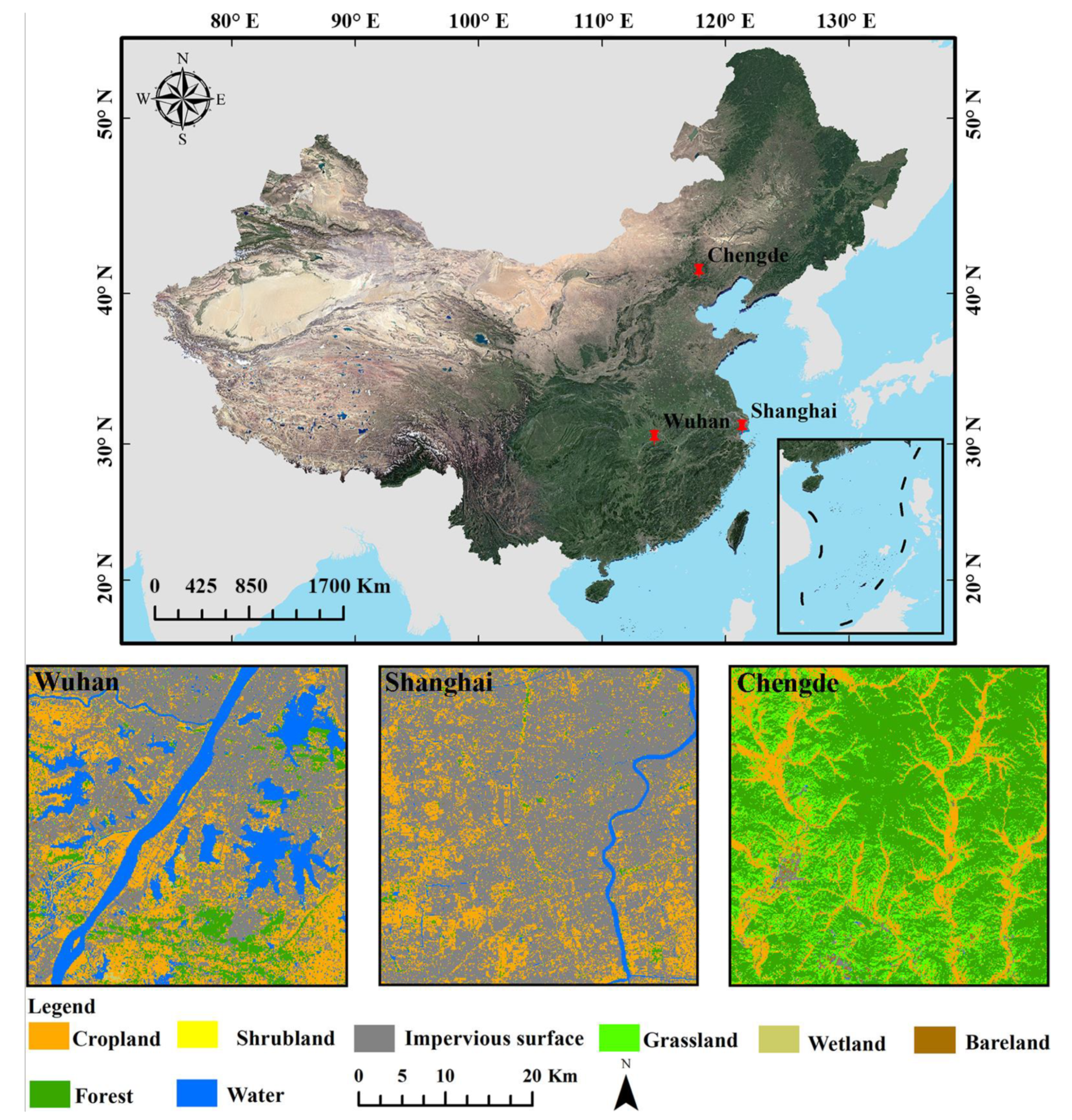
2.1. Study Area
2.2. Data and Data Preprocessing
2.3. Random Forest Regression
2.4. Feature Selection
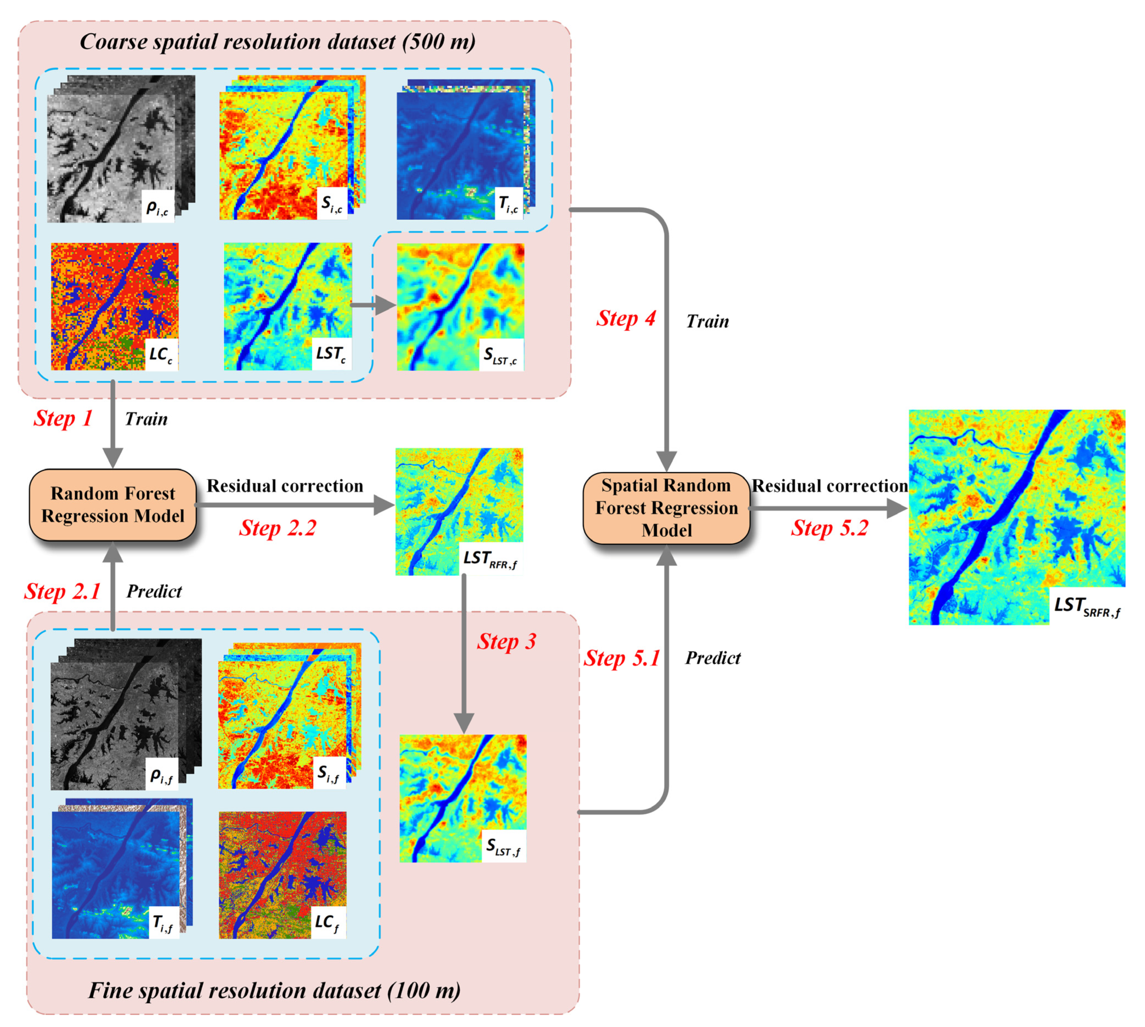
2.5. Spatial Random Forest LST Downscaling Method
- Obtaining the trained RFR model () using the LST and predictor variable dataset at a coarse spatial resolution, excluding the spatial feature of the LST ().
- Obtaining the downscaled LST image with a fine spatial resolution () by applying the predictor variable dataset with a fine spatial resolution to the and performing the residual correction.
- Obtaining the spatial feature of LST with a fine spatial resolution () by Equation (7) based on .
- Obtaining the trained spatial RFR () using the LST and predictor variable dataset at a coarse spatial resolution, including the .
- Obtaining the final downscaled LST image by applying the predictor variable dataset with a fine spatial resolution to the and performing the residual correction.
2.6. Validation Methods
3. Results and Analysis
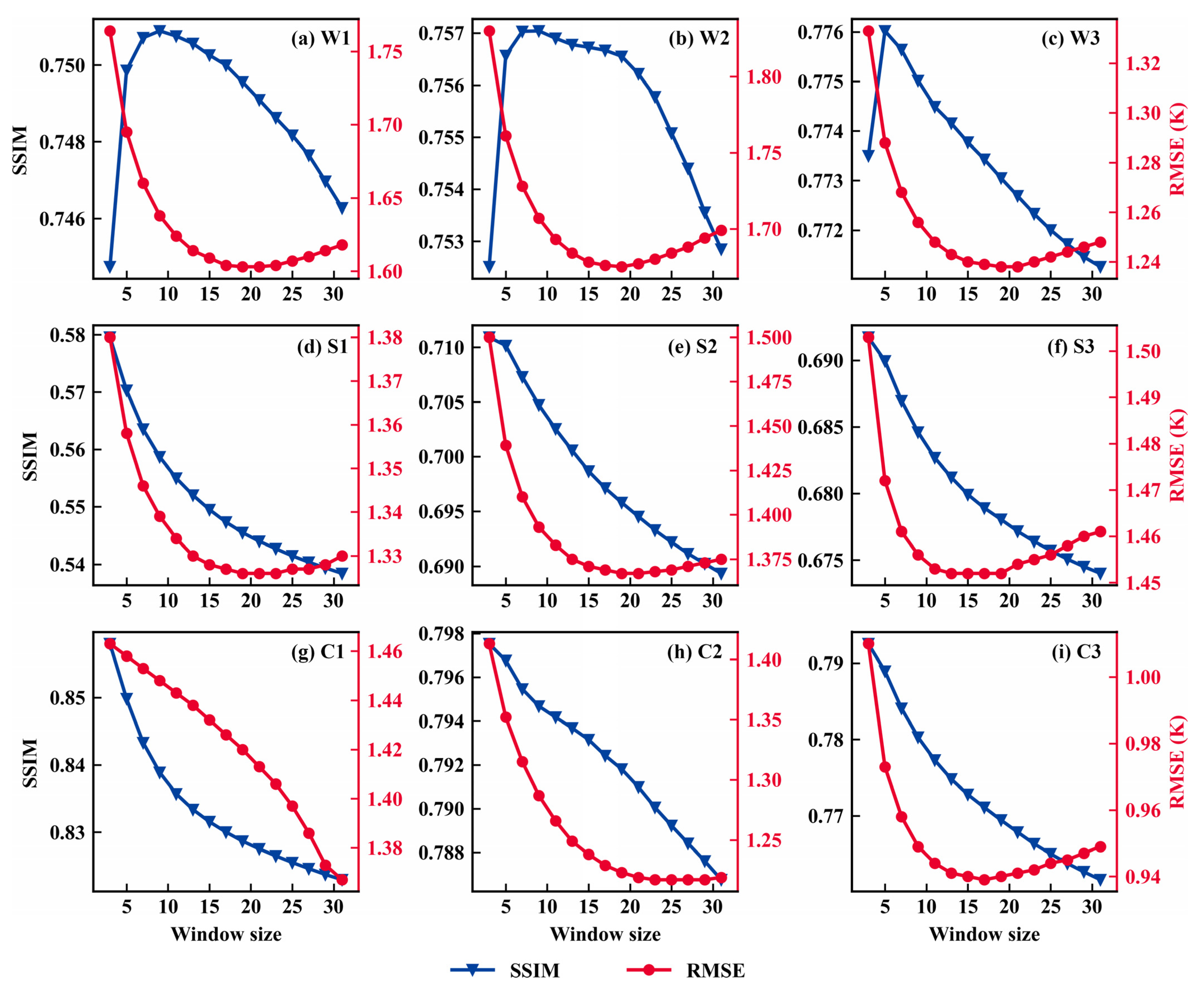
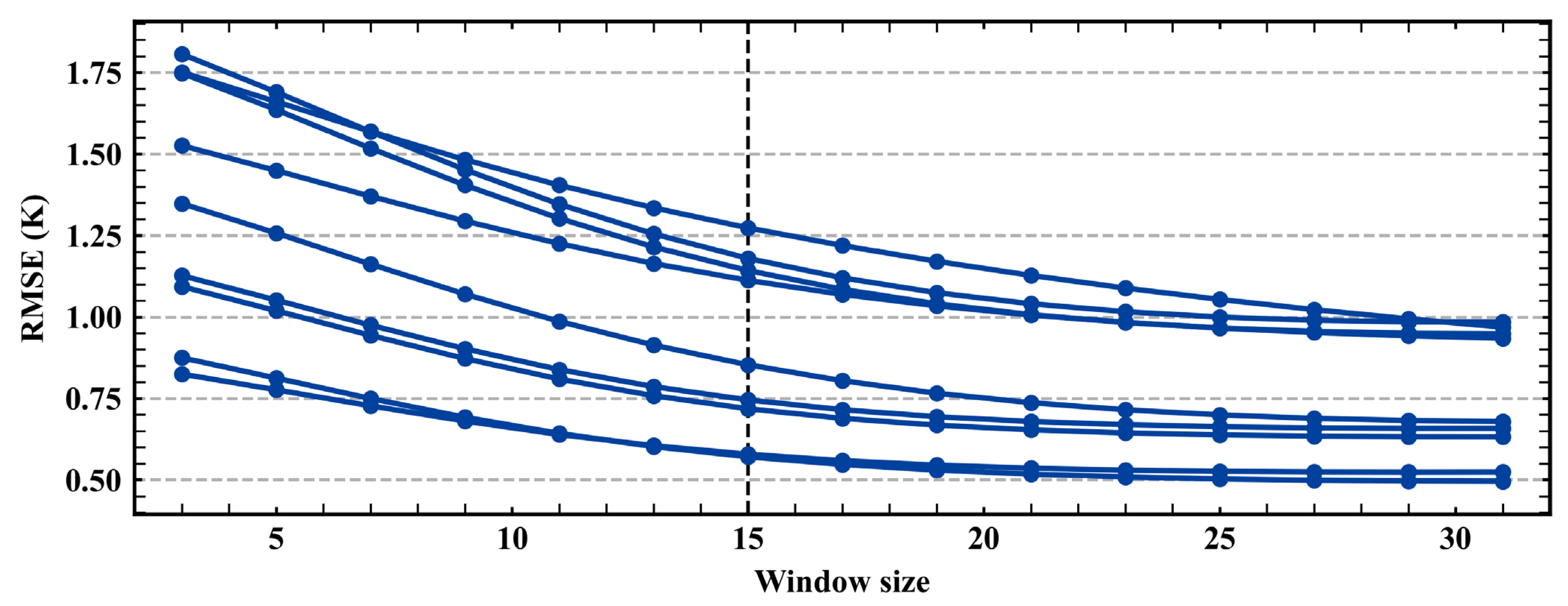
3.1. Determination of the Window Size for Calculating Spatial Feature of the LST
3.1.1. Window Size of Coarse-Resolution LST Image
3.1.2. Window Size of Fine-Resolution LST Image
3.2. Downscaling Results
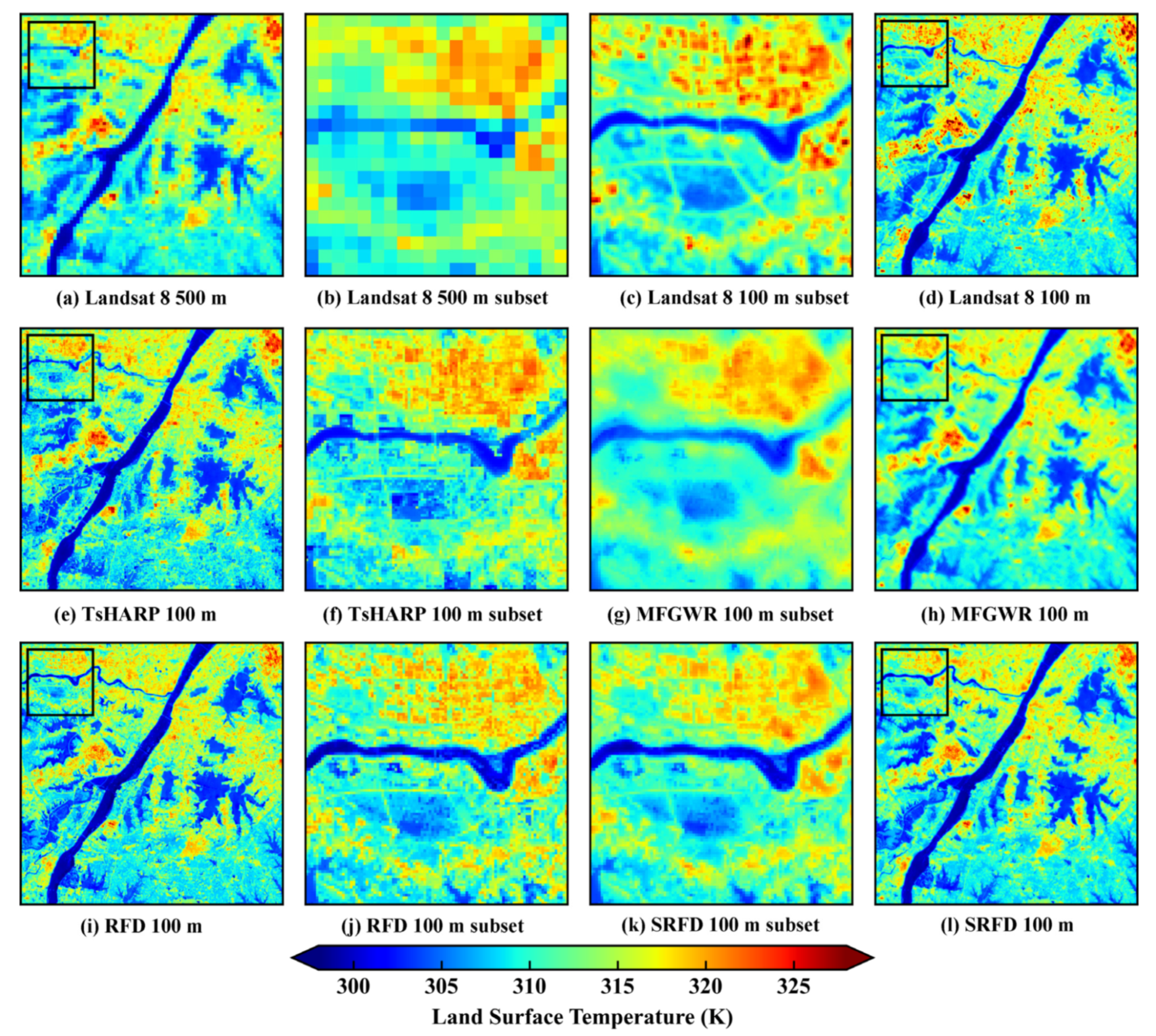
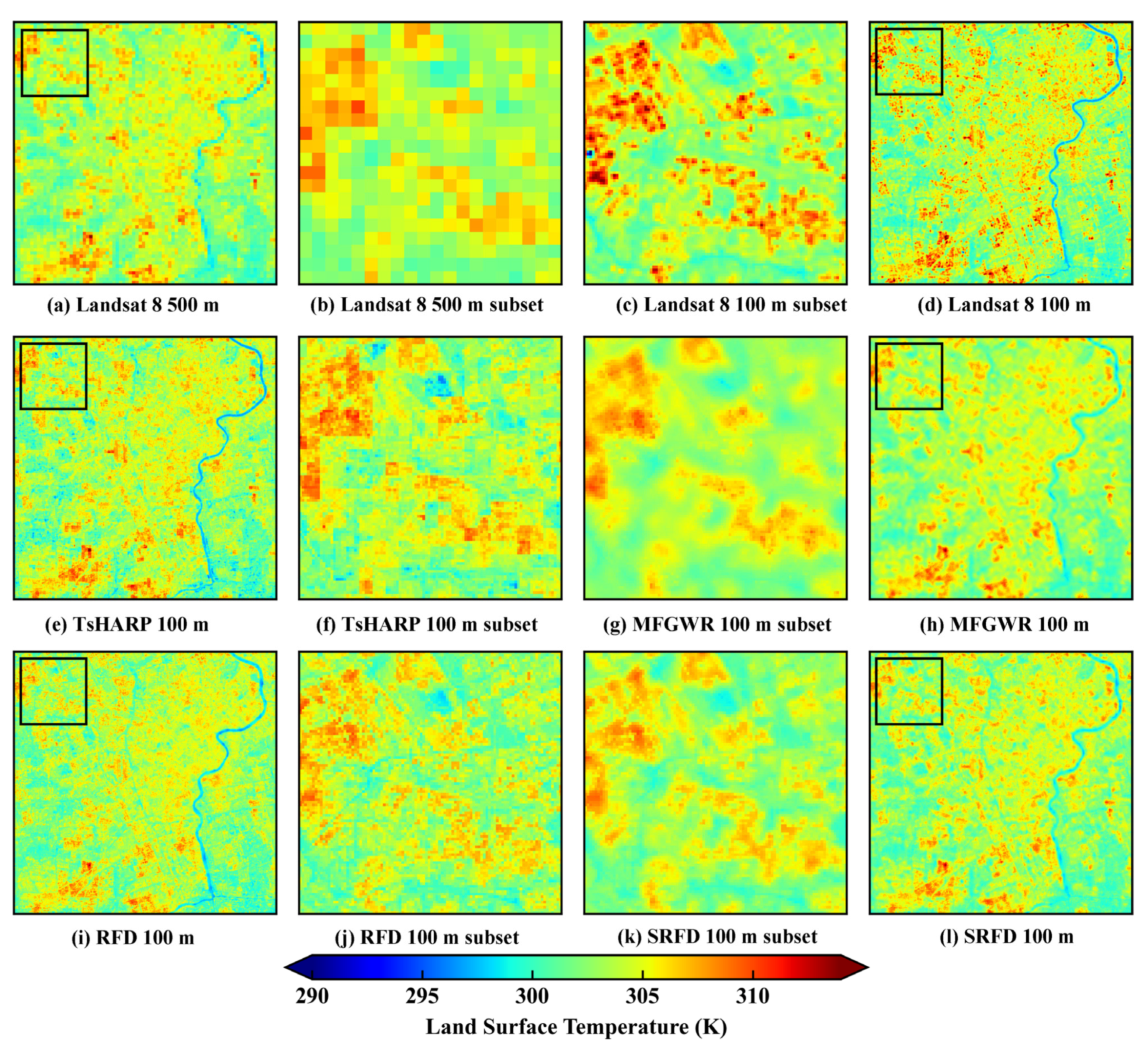
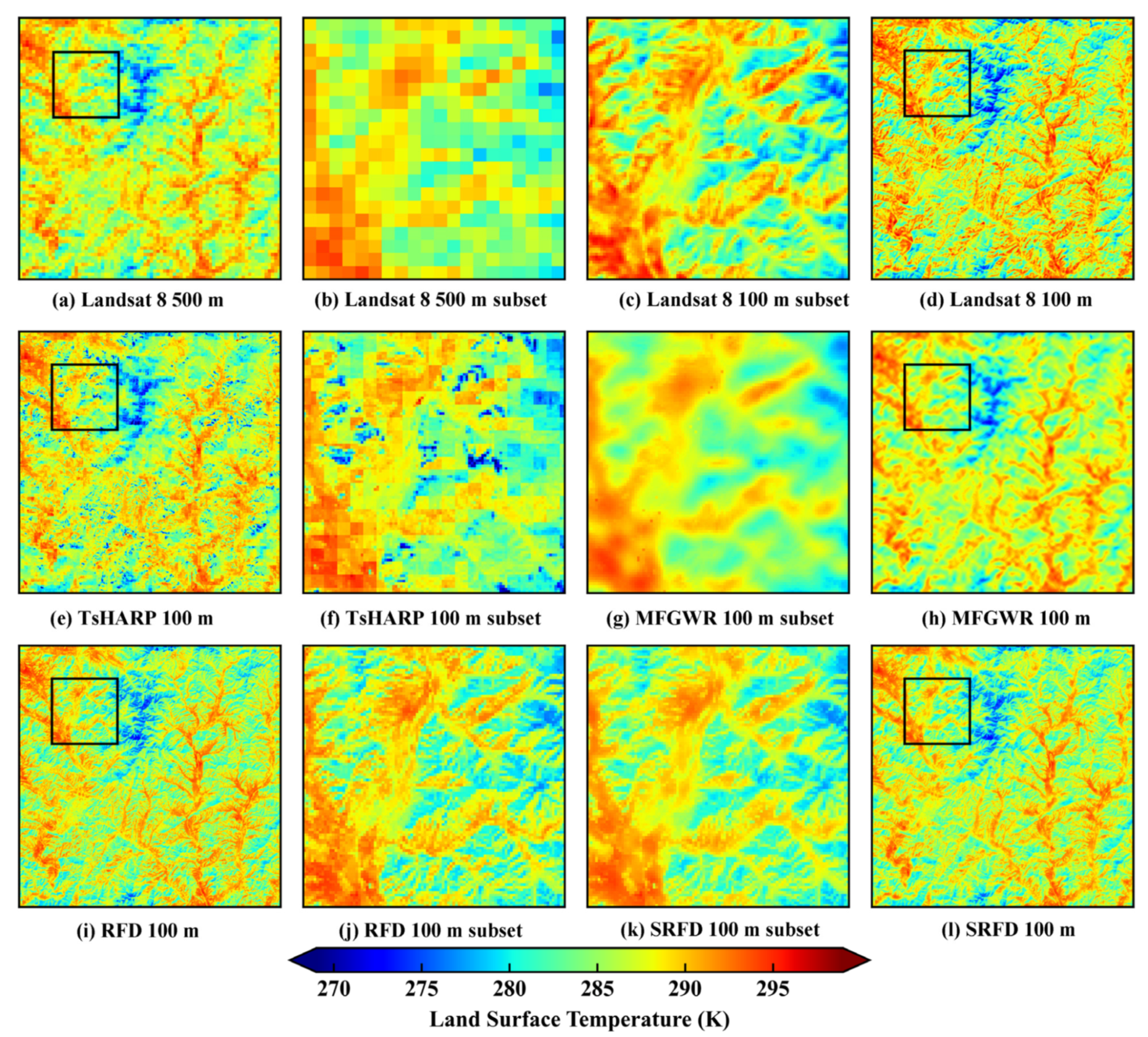
3.2.1. Visual Evaluation
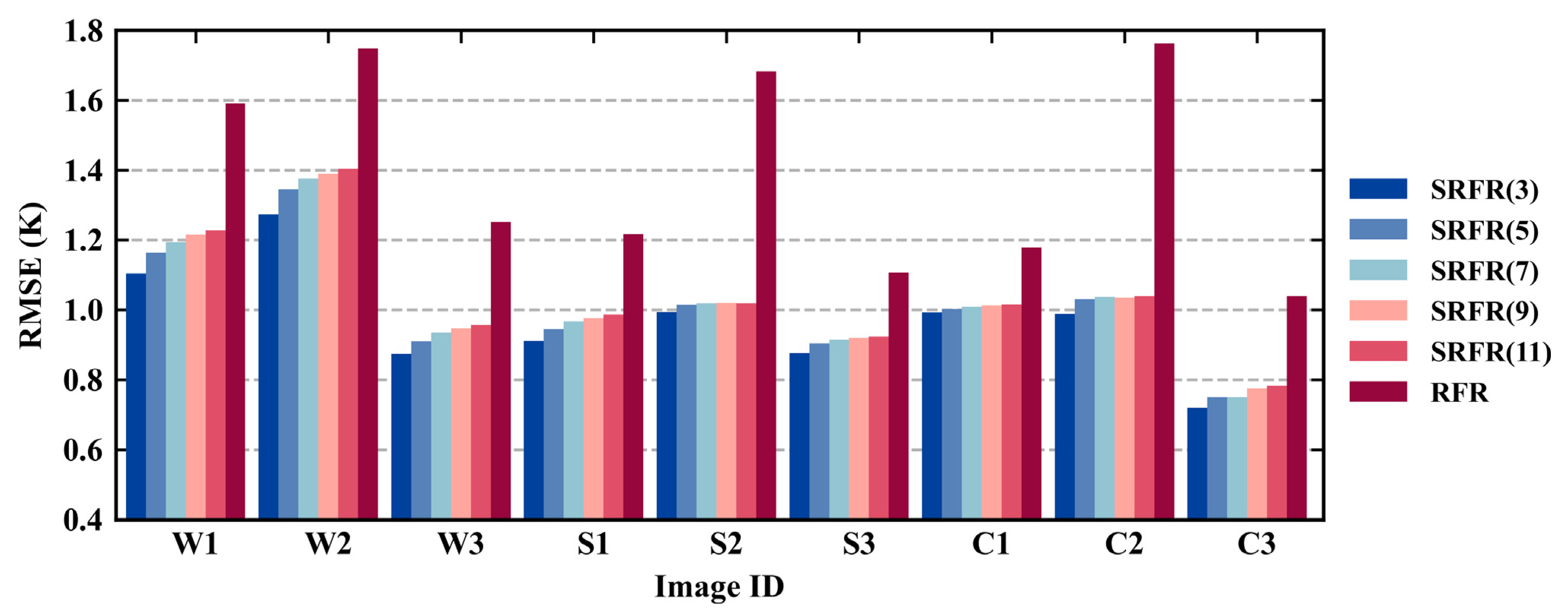
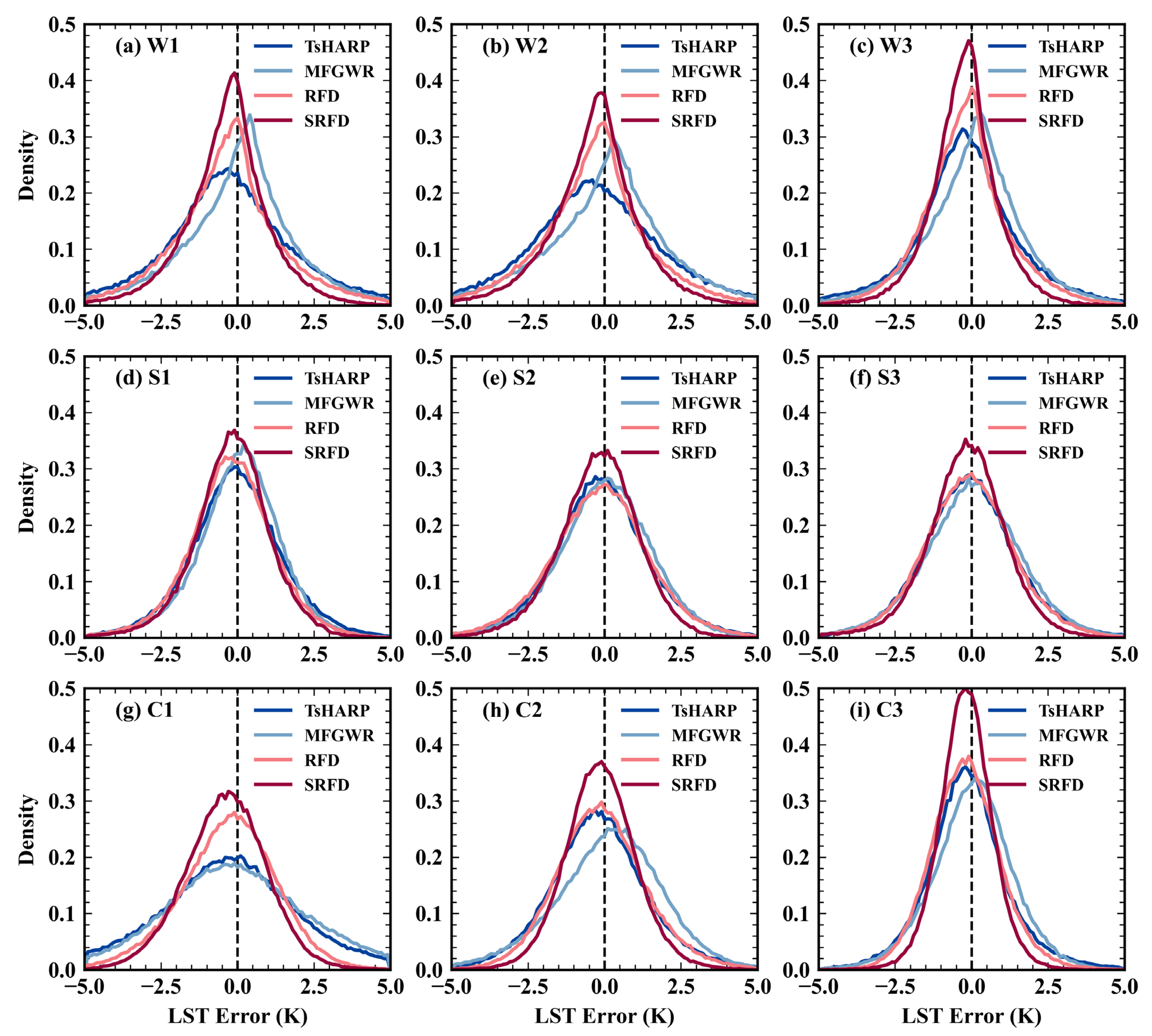
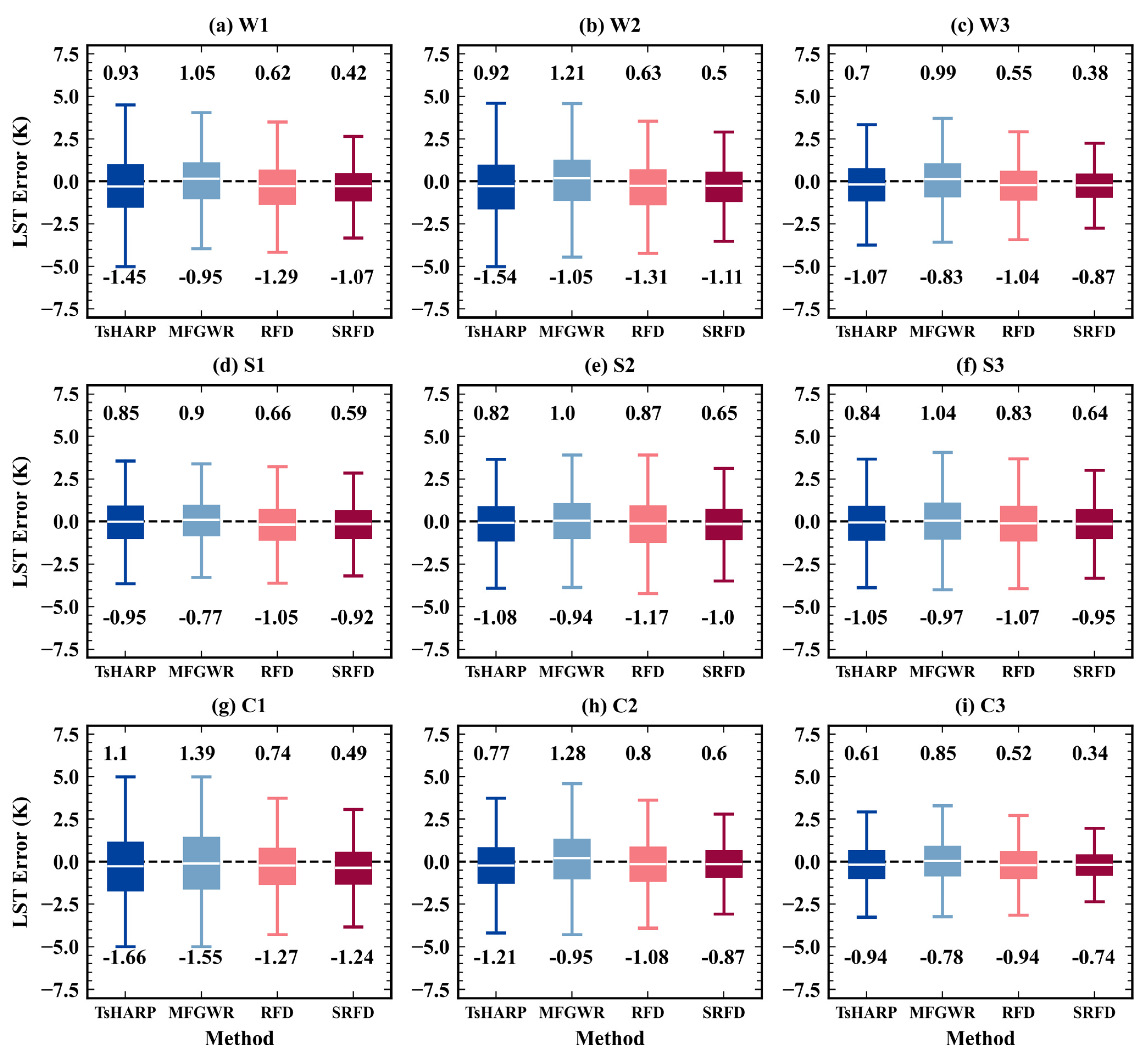
3.2.2. Quantitative Evaluation
4. Discussion
4.1. Error Characteristics of the SRFD
4.2. Error Sources of the SRFD
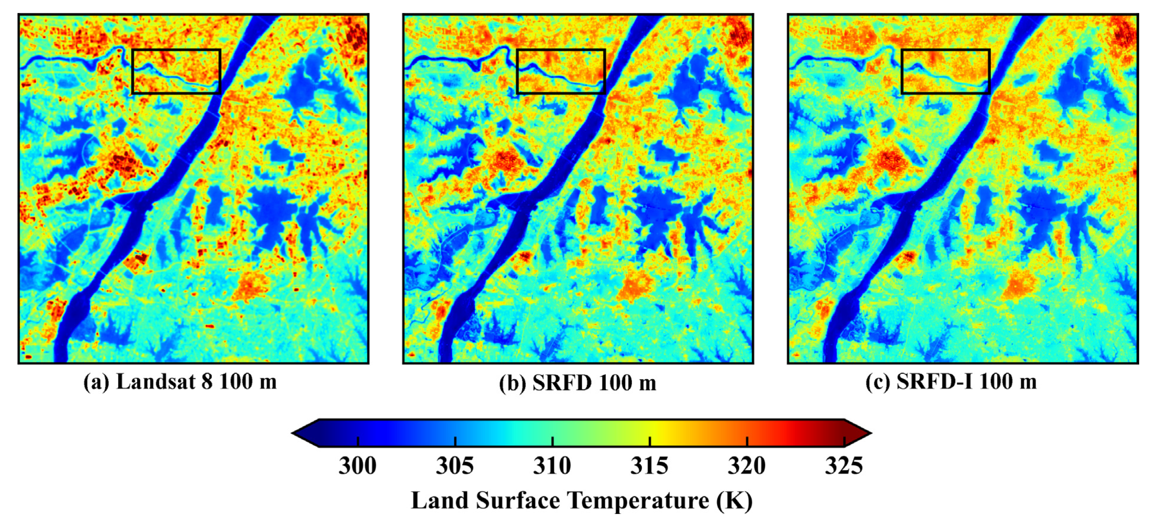
4.3. Difference of the Way to Obtain Fine-Resolution Spatial Feature Image
5. Conclusions
Author Contributions
Funding
Institutional Review Board Statement
Informed Consent Statement
Acknowledgments
Conflicts of Interest
References
- Weng, Q. Thermal infrared remote sensing for urban climate and environmental studies: Methods, applications, and trends. ISPRS J. Photogramm. Remote Sens. 2009, 64, 335–344. [Google Scholar] [CrossRef]
- Li, Z.-L.; Tang, B.-H.; Wu, H.; Ren, H.; Yan, G.; Wan, Z.; Trigo, I.F.; Sobrino, J.A. Satellite-derived land surface temperature: Current status and perspectives. Remote Sens. Environ. 2013, 131, 14–37. [Google Scholar] [CrossRef] [Green Version]
- Duan, S.-B.; Li, Z.-L.; Tang, B.-H.; Wu, H.; Tang, R. Generation of a time-consistent land surface temperature product from MODIS data. Remote Sens. Environ. 2014, 140, 339–349. [Google Scholar] [CrossRef]
- Cao, B.; Liu, Q.; Du, Y.; Roujean, J.-L.; Gastellu-Etchegorry, J.-P.; Trigo, I.F.; Zhan, W.; Yu, Y.; Cheng, J.; Jacob, F.; et al. A review of earth surface thermal radiation directionality observing and modeling: Historical development, current status and perspectives. Remote Sens. Environ. 2019, 232, 111304. [Google Scholar] [CrossRef]
- Zhu, X.; Cai, F.; Tian, J.; Williams, T. Spatiotemporal fusion of multisource remote sensing data: Literature survey, taxonomy, principles, applications, and future directions. Remote Sens. 2018, 10, 527. [Google Scholar] [CrossRef] [Green Version]
- Wan, Z.; Li, Z.L. Radiance-based validation of the V5 MODIS land-surface temperature product. Int. J. Remote Sens. 2010, 29, 5373–5395. [Google Scholar] [CrossRef]
- Merlin, O.; Duchemin, B.; Hagolle, O.; Jacob, F.; Coudert, B.; Chehbouni, G.; Dedieu, G.; Garatuza, J.; Kerr, Y. Disaggregation of MODIS surface temperature over an agricultural area using a time series of Formosat-2 images. Remote Sens. Environ. 2010, 114, 2500–2512. [Google Scholar] [CrossRef] [Green Version]
- Jimenez-Munoz, J.C.; Sobrino, J.A. Feasibility of retrieving land-surface temperature from ASTER TIR bands using two-channel algorithms: A case study of agricultural areas. IEEE Geosci. Remote Sens. Lett. 2007, 4, 60–64. [Google Scholar] [CrossRef]
- Zhan, W.; Chen, Y.; Zhou, J.; Wang, J.; Liu, W.; Voogt, J.; Zhu, X.; Quan, J.; Li, J. Disaggregation of remotely sensed land surface temperature: Literature survey, taxonomy, issues, and caveats. Remote Sens. Environ. 2013, 131, 119–139. [Google Scholar] [CrossRef]
- Tang, B.-H.; Shao, K.; Li, Z.-L.; Wu, H.; Nerry, F.; Zhou, G. Estimation and validation of land surface temperatures from Chinese second-generation polar-orbit FY-3A VIRR data. Remote Sens. 2015, 7, 3250–3273. [Google Scholar] [CrossRef] [Green Version]
- Jiang, J.; Li, H.; Liu, Q.; Wang, H.; Du, Y.; Cao, B.; Zhong, B.; Wu, S. Evaluation of land surface temperature retrieval from FY-3B/VIRR data in an arid area of Northwestern China. Remote Sens. 2015, 7, 7080–7104. [Google Scholar] [CrossRef] [Green Version]
- Meng, X.; Cheng, J.; Liang, S. Estimating land surface temperature from Feng Yun-3C/MERSI data using a new land surface emissivity scheme. Remote Sens. 2017, 9, 1247. [Google Scholar] [CrossRef] [Green Version]
- Tang, K.; Zhu, H.; Ni, P.; Li, R.; Fan, C. Retrieving land surface temperature from Chinese FY-3D MERSI-2 data using an operational split window algorithm. IEEE J. Sel. Top. Appl. Earth Obs. Remote Sens. 2021, 14, 6639–6651. [Google Scholar] [CrossRef]
- Wang, H.; Mao, K.; Mu, F.; Shi, J.; Yang, J.; Li, Z.; Qin, Z. A split window algorithm for retrieving land surface temperature from FY-3D MERSI-2 data. Remote Sens. 2019, 11, 2083. [Google Scholar] [CrossRef] [Green Version]
- Mao, Q.; Peng, J.; Wang, Y. Resolution enhancement of remotely sensed land surface temperature: Current status and perspectives. Remote Sens. 2021, 13, 1306. [Google Scholar] [CrossRef]
- Xia, H.; Chen, Y.; Li, Y.; Quan, J. Combining kernel-driven and fusion-based methods to generate daily high-spatial-resolution land surface temperatures. Remote Sens. Environ. 2019, 224, 259–274. [Google Scholar] [CrossRef]
- Feng, G.; Masek, J.; Schwaller, M.; Hall, F. On the blending of the Landsat and MODIS surface reflectance: Predicting daily Landsat surface reflectance. IEEE Trans. Geosci. Remote Sens. 2006, 44, 2207–2218. [Google Scholar] [CrossRef]
- Wu, P.; Yin, Z.; Zeng, C.; Duan, S.-B.; Gottsche, F.-M.; Li, X.; Ma, X.; Yang, H.; Shen, H. Spatially continuous and high-resolution land surface temperature product generation: A review of reconstruction and spatiotemporal fusion techniques. IEEE Geosci. Remote Sens. Mag. 2021. [Google Scholar] [CrossRef]
- Zhu, X.; Chen, J.; Gao, F.; Chen, X.; Masek, J.G. An enhanced spatial and temporal adaptive reflectance fusion model for complex heterogeneous regions. Remote Sens. Environ. 2010, 114, 2610–2623. [Google Scholar] [CrossRef]
- Liu, H.; Weng, Q. Enhancing temporal resolution of satellite imagery for public health studies: A case study of West Nile Virus outbreak in Los Angeles in 2007. Remote Sens. Environ. 2012, 117, 57–71. [Google Scholar] [CrossRef]
- Yang, G.; Weng, Q.; Pu, R.; Gao, F.; Sun, C.; Li, H.; Zhao, C. Evaluation of ASTER-Like daily land surface temperature by fusing ASTER and MODIS data during the HiWATER-MUSOEXE. Remote Sens. 2016, 8, 75. [Google Scholar] [CrossRef] [Green Version]
- Weng, Q.; Fu, P.; Gao, F. Generating daily land surface temperature at Landsat resolution by fusing Landsat and MODIS data. Remote Sens. Environ. 2014, 145, 55–67. [Google Scholar] [CrossRef]
- Niu, Z. Use of MODIS and Landsat time series data to generate high-resolution temporal synthetic Landsat data using a spatial and temporal reflectance fusion model. J. Appl. Remote Sens. 2012, 6, 63507. [Google Scholar] [CrossRef]
- Wu, M.; Huang, W.; Niu, Z.; Wang, C. Generating daily synthetic Landsat imagery by combining Landsat and MODIS data. Sensors 2015, 15, 24002–24025. [Google Scholar] [CrossRef] [PubMed] [Green Version]
- Zurita-Milla, R.; Clevers, J.; Schaepman, M.E. Unmixing-based Landsat TM and MERIS FR data fusion. IEEE Geosci. Remote Sens. Lett. 2008, 5, 453–457. [Google Scholar] [CrossRef] [Green Version]
- Gevaert, C.M.; García-Haro, F.J. A comparison of STARFM and an unmixing-based algorithm for Landsat and MODIS data fusion. Remote Sens. Environ. 2015, 156, 34–44. [Google Scholar] [CrossRef]
- Zhu, X.; Helmer, E.H.; Gao, F.; Liu, D.; Chen, J.; Lefsky, M.A. A flexible spatiotemporal method for fusing satellite images with different resolutions. Remote Sens. Environ. 2016, 172, 165–177. [Google Scholar] [CrossRef]
- Li, X.; Ling, F.; Foody, G.M.; Ge, Y.; Zhang, Y.; Du, Y. Generating a series of fine spatial and temporal resolution land cover maps by fusing coarse spatial resolution remotely sensed images and fine spatial resolution land cover maps. Remote Sens. Environ. 2017, 196, 293–311. [Google Scholar] [CrossRef]
- Choe, Y.-J.; Yom, J.-H. Improving accuracy of land surface temperature prediction model based on deep-learning. Spat. Inf. Res. 2019, 28, 377–382. [Google Scholar] [CrossRef]
- Yin, Z.; Wu, P.; Foody, G.M.; Wu, Y.; Liu, Z.; Du, Y.; Ling, F. Spatiotemporal fusion of land surface temperature based on a convolutional neural network. IEEE Trans. Geosci. Remote Sens. 2020, 59, 1808–1822. [Google Scholar] [CrossRef]
- Liu, Y.; Hiyama, T.; Yamaguchi, Y. Scaling of land surface temperature using satellite data: A case examination on ASTER and MODIS products over a heterogeneous terrain area. Remote Sens. Environ. 2006, 105, 115–128. [Google Scholar] [CrossRef]
- Guo, L.J.; Moore, J.M. Pixel block intensity modulation: Adding spatial detail to TM band 6 thermal imagery. Int. J. Remote Sens. 2010, 19, 2477–2491. [Google Scholar] [CrossRef]
- Nichol, J. An emissivity modulation method for spatial enhancement of thermal satellite images in urban heat island analysis. Photogramm. Eng. Remote Sens. 2009, 75, 547–556. [Google Scholar] [CrossRef] [Green Version]
- Agam, N.; Kustas, W.P.; Anderson, M.C.; Li, F.; Neale, C.M.U. A vegetation index based technique for spatial sharpening of thermal imagery. Remote Sens. Environ. 2007, 107, 545–558. [Google Scholar] [CrossRef]
- Kustas, W.P.; Norman, J.M.; Anderson, M.C.; French, A.N. Estimating subpixel surface temperatures and energy fluxes from the vegetation index–radiometric temperature relationship. Remote Sens. Environ. 2003, 85, 429–440. [Google Scholar] [CrossRef]
- Dominguez, A.; Kleissl, J.; Luvall, J.C.; Rickman, D.L. High-resolution urban thermal sharpener (HUTS). Remote Sens. Environ. 2011, 115, 1772–1780. [Google Scholar] [CrossRef] [Green Version]
- Duan, S.-B.; Li, Z.-L. Spatial downscaling of MODIS land surface temperatures using geographically weighted regression: Case Study in Northern China. IEEE Trans. Geosci. Remote Sens. 2016, 54, 6458–6469. [Google Scholar] [CrossRef]
- Wu, J.; Zhong, B.; Tian, S.; Yang, A.; Wu, J. Downscaling of urban land surface temperature based on multi-factor geographically weighted regression. IEEE J. Sel. Top. Appl. Earth Obs. Remote Sens. 2019, 12, 2897–2911. [Google Scholar] [CrossRef]
- Wang, S.; Luo, Y.; Li, X.; Yang, K.; Liu, Q.; Luo, X.; Li, X. Downscaling land surface temperature based on non-linear geographically weighted regressive model over urban areas. Remote Sens. 2021, 13, 1580. [Google Scholar] [CrossRef]
- Hutengs, C.; Vohland, M. Downscaling land surface temperatures at regional scales with random forest regression. Remote Sens. Environ. 2016, 178, 127–141. [Google Scholar] [CrossRef]
- Pan, X.; Zhu, X.; Yang, Y.; Cao, C.; Zhang, X.; Shan, L. Applicability of downscaling land surface temperature by using normalized difference sand index. Sci. Rep. 2018, 8, 9530. [Google Scholar] [CrossRef] [Green Version]
- Zhao, W.; Duan, S.-B. Reconstruction of daytime land surface temperatures under cloud-covered conditions using integrated MODIS/Terra land products and MSG geostationary satellite data. Remote Sens. Environ. 2020, 247, 111931. [Google Scholar] [CrossRef]
- Yang, Y.; Cao, C.; Pan, X.; Li, X.; Zhu, X. Downscaling land surface temperature in an arid area by using multiple remote sensing indices with random forest regression. Remote Sens. 2017, 9, 789. [Google Scholar] [CrossRef] [Green Version]
- Zawadzka, J.; Corstanje, R.; Harris, J.; Truckell, I. Downscaling Landsat-8 land surface temperature maps in diverse urban landscapes using multivariate adaptive regression splines and very high resolution auxiliary data. Int. J. Digit. Earth 2019, 13, 899–914. [Google Scholar] [CrossRef] [Green Version]
- Liu, Y.; Jing, W.; Wang, Q.; Xia, X. Generating high-resolution daily soil moisture by using spatial downscaling techniques: A comparison of six machine learning algorithms. Adv. Water Resour. 2020, 141, 103601. [Google Scholar] [CrossRef]
- Bartkowiak, P.; Castelli, M.; Notarnicola, C. Downscaling land surface temperature from MODIS dataset with random forest approach over alpine vegetated areas. Remote Sens. 2019, 11, 1319. [Google Scholar] [CrossRef] [Green Version]
- Ebrahimy, H.; Azadbakht, M. Downscaling MODIS land surface temperature over a heterogeneous area: An investigation of machine learning techniques, feature selection, and impacts of mixed pixels. Comput. Geosci. 2019, 124, 93–102. [Google Scholar] [CrossRef]
- Li, W.; Ni, L.; Li, Z.L.; Duan, S.B.; Wu, H. Evaluation of machine learning algorithms in spatial downscaling of MODIS land surface temperature. IEEE J. Sel. Top. Appl. Earth Obs. Remote Sens. 2019, 12, 2299–2307. [Google Scholar] [CrossRef]
- Xu, S.; Zhao, Q.; Yin, K.; He, G.; Zhang, Z.; Wang, G.; Wen, M.; Zhang, N. Spatial downscaling of land surface temperature based on a multi-factor geographically weighted machine learning model. Remote Sens. 2021, 13, 1186. [Google Scholar] [CrossRef]
- Li, T.; Shen, H.; Yuan, Q.; Zhang, X.; Zhang, L. Estimating ground-level PM2.5by fusing satellite and station observations: A Geo-intelligent deep learning approach. Geophys. Res. Lett. 2017, 44, 11985–11993. [Google Scholar] [CrossRef] [Green Version]
- Wei, J.; Huang, W.; Li, Z.; Xue, W.; Peng, Y.; Sun, L.; Cribb, M. Estimating 1-km-resolution PM2.5 concentrations across China using the space-time random forest approach. Remote Sens. Environ. 2019, 231, 111221. [Google Scholar] [CrossRef]
- Loveland, T.R.; Irons, J.R. Landsat 8: The plans, the reality, and the legacy. Remote Sens. Environ. 2016, 185, 1–6. [Google Scholar] [CrossRef] [Green Version]
- Vermote, E.; Justice, C.; Claverie, M.; Franch, B. Preliminary analysis of the performance of the Landsat 8/OLI land surface reflectance product. Remote Sens. Environ. 2016, 185, 46–56. [Google Scholar] [CrossRef] [PubMed]
- Montanaro, M.; Gerace, A.; Lunsford, A.; Reuter, D. Stray light artifacts in imagery from the Landsat 8 thermal infrared sensor. Remote Sens. 2014, 6, 10435–10456. [Google Scholar] [CrossRef] [Green Version]
- Montanaro, M.; Lunsford, A.; Tesfaye, Z.; Wenny, B.; Reuter, D. Radiometric calibration methodology of the Landsat 8 thermal infrared sensor. Remote Sens. 2014, 6, 8803–8821. [Google Scholar] [CrossRef] [Green Version]
- Malakar, N.K.; Hulley, G.C.; Hook, S.J.; Laraby, K.; Cook, M.; Schott, J.R. An operational land surface temperature product for Landsat thermal data: Methodology and validation. IEEE Trans. Geosci. Remote Sens. 2018, 56, 5717–5735. [Google Scholar] [CrossRef]
- Barsi, J.A.; Barker, J.L.; Schott, J.R. An atmospheric correction parameter calculator for a single thermal band earth-sensing instrument. In Proceedings of the 2003 IEEE International Geoscience and Remote Sensing Symposium, Toulouse, France, 21–25 July 2003; Volume 3015, pp. 3014–3016. [Google Scholar]
- Barsi, J.A.; Butler, J.J.; Schott, J.R.; Palluconi, F.D.; Hook, S.J. Validation of a web-based atmospheric correction tool for single thermal band instruments. In Proceedings of the Earth Observing Systems X, San Diego, CA, USA, 31 July–2 August 2005. [Google Scholar]
- Sobrino, J.A.; Jimenez-Munoz, J.C.; Soria, G.; Romaguera, M.; Guanter, L.; Moreno, J.; Plaza, A.; Martinez, P. Land surface emissivity retrieval from different VNIR and TIR sensors. IEEE Trans. Geosci. Remote Sens. 2008, 46, 316–327. [Google Scholar] [CrossRef]
- Wang, F.; Qin, Z.; Song, C.; Tu, L.; Karnieli, A.; Zhao, S. An improved Mono-window algorithm for land surface temperature retrieval from Landsat 8 thermal infrared sensor data. Remote Sens. 2015, 7, 4268–4289. [Google Scholar] [CrossRef] [Green Version]
- Yang, L.; Meng, X.; Zhang, X. SRTM DEM and its application advances. Int. J. Remote Sens. 2011, 32, 3875–3896. [Google Scholar] [CrossRef]
- Gong, P.; Wang, J.; Yu, L.; Zhao, Y.; Zhao, Y.; Liang, L.; Niu, Z.; Huang, X.; Fu, H.; Liu, S.; et al. Finer resolution observation and monitoring of global land cover: First mapping results with Landsat TM and ETM+ data. Int. J. Remote Sens. 2012, 34, 2607–2654. [Google Scholar] [CrossRef] [Green Version]
- Desheng, L.; Xiaolin, Z. An enhanced physical method for downscaling thermal infrared radiance. IEEE Geosci. Remote Sens. Lett. 2012, 9, 690–694. [Google Scholar] [CrossRef]
- Breiman, L. Random forests. Mach. Learn. 2001, 45, 5–32. [Google Scholar] [CrossRef] [Green Version]
- Hastie, T.; Tibshirani, R.; Friedman, J. The Elements of Statistical Learning; Springer: Berlin/Heidelberg, Germany, 2009. [Google Scholar]
- Wang, H.; Magagi, R.; Goïta, K.; Trudel, M.; McNairn, H.; Powers, J. Crop phenology retrieval via polarimetric SAR decomposition and Random Forest algorithm. Remote Sens. Environ. 2019, 231, 111234. [Google Scholar] [CrossRef]
- Tong, C.; Wang, H.; Magagi, R.; Goïta, K.; Zhu, L.; Yang, M.; Deng, J. Soil moisture retrievals by combining passive microwave and optical data. Remote Sens. 2020, 12, 3173. [Google Scholar] [CrossRef]
- Krstajic, D.; Buturovic, L.J.; Leahy, D.E.; Thomas, S. Cross-validation pitfalls when selecting and assessing regression and classification models. J. Cheminform. 2014, 6, 10. [Google Scholar] [CrossRef] [PubMed] [Green Version]
- Rikimaru, A.; Roy, P.; Miyatake, S. Tropical forest cover density mapping. Trop. Ecol. 2002, 43, 39–47. [Google Scholar]
- Qi, J.; Chehbouni, A.; Huete, A.R.; Kerr, Y.H.; Sorooshian, S. A modified soil adjusted vegetation index. Remote Sens. Environ. 1994, 48, 119–126. [Google Scholar] [CrossRef]
- Zha, Y.; Gao, J.; Ni, S. Use of normalized difference built-up index in automatically mapping urban areas from TM imagery. Int. J. Remote Sens. 2003, 24, 583–594. [Google Scholar] [CrossRef]
- Gu, Y.; Brown, J.F.; Verdin, J.P.; Wardlow, B. A five-year analysis of MODIS NDVI and NDWI for grassland drought assessment over the central Great Plains of the United States. Geophys. Res. Lett. 2007, 34. [Google Scholar] [CrossRef] [Green Version]
- Pettorelli, N.; Vik, J.O.; Mysterud, A.; Gaillard, J.M.; Tucker, C.J.; Stenseth, N.C. Using the satellite-derived NDVI to assess ecological responses to environmental change. Trends Ecol. Evol. 2005, 20, 503–510. [Google Scholar] [CrossRef]
- McFeeters, S.K. The use of the Normalized Difference Water Index (NDWI) in the delineation of open water features. Int. J. Remote Sens. 2007, 17, 1425–1432. [Google Scholar] [CrossRef]
- Xu, H. Modification of normalised difference water index (NDWI) to enhance open water features in remotely sensed imagery. Int. J. Remote Sens. 2007, 27, 3025–3033. [Google Scholar] [CrossRef]
- Rondeaux, G.; Steven, M.; Baret, F. Optimization of soil-adjusted vegetation indices. Remote Sens. Environ. 1996, 55, 95–107. [Google Scholar] [CrossRef]
- Huete, A.R. A soil-adjusted vegetation index (SAVI). Remote Sens. Environ. 1988, 25, 295–309. [Google Scholar] [CrossRef]
- Xu, H. A new index for delineating built-up land features in satellite imagery. Int. J. Remote Sens. 2008, 29, 4269–4276. [Google Scholar] [CrossRef]
- Villa, P. Imperviousness indexes performance evaluation for mapping urban areas using remote sensing data. In Proceedings of the 2007 Urban Remote Sensing Joint Event, Paris, France, 11–13 April 2007; pp. 1–6. [Google Scholar]
- Brunsdon, C.; Fotheringham, S.; Charlton, M. Geographically weighted regression. J. R. Stat. Soc. Ser. D 1998, 47, 431–443. [Google Scholar] [CrossRef]
- O’brien, R.M. A caution regarding rules of thumb for variance inflation factors. Qual. Quant. 2007, 41, 673–690. [Google Scholar] [CrossRef]
- Niazian, M.; Sadat-Noori, S.A.; Abdipour, M. Modeling the seed yield of Ajowan (Trachyspermum ammi L.) using artificial neural network and multiple linear regression models. Ind. Crop. Prod. 2018, 117, 224–234. [Google Scholar] [CrossRef]
- Feng, L.; Wang, Y.; Zhang, Z.; Du, Q. Geographically and temporally weighted neural network for winter wheat yield prediction. Remote Sens. Environ. 2021, 262. [Google Scholar] [CrossRef]
- Otsu, N. A threshold selection method from gray-level histograms. IEEE Trans. Syst. Man Cybern. 1979, 9, 62–66. [Google Scholar] [CrossRef] [Green Version]
- Wang, Z.; Bovik, A.C.; Sheikh, H.R.; Simoncelli, E.P. Image quality assessment: From error visibility to structural similarity. IEEE Trans. Image Process. 2004, 13, 600–612. [Google Scholar] [CrossRef] [Green Version]
- Tobler, W.R. A computer movie simulating urban growth in the detroit region. Econ. Geogr. 1970, 46, 234–240. [Google Scholar] [CrossRef]
- Njuki, S.M.; Mannaerts, C.M.; Su, Z. An improved approach for downscaling coarse-resolution thermal data by minimizing the spatial averaging biases in random forest. Remote Sens. 2020, 12, 3507. [Google Scholar] [CrossRef]
- Zheng, X.; Gao, M.; Li, Z.-L.; Chen, K.-S.; Zhang, X.; Shang, G. Impact of 3-D structures and their radiation on thermal infrared measurements in urban areas. IEEE Trans. Geosci. Remote Sens. 2020, 58, 8412–8426. [Google Scholar] [CrossRef]
- Chen, S.; Ren, H.; Ye, X.; Dong, J.; Zheng, Y. Geometry and adjacency effects in urban land surface temperature retrieval from high-spatial-resolution thermal infrared images. Remote Sens. Environ. 2021, 262, 112518. [Google Scholar] [CrossRef]
- Xue, T.; Zheng, Y.; Geng, G.; Zheng, B.; Jiang, X.; Zhang, Q.; He, K. Fusing observational, satellite remote sensing and air quality model simulated data to estimate spatiotemporal variations of PM2.5 exposure in China. Remote Sens. 2017, 9, 221. [Google Scholar] [CrossRef] [Green Version]
- Liang, F.; Xiao, Q.; Wang, Y.; Lyapustin, A.; Li, G.; Gu, D.; Pan, X.; Liu, Y. MAIAC-based long-term spatiotemporal trends of PM2.5 in Beijing, China. Sci. Total Environ 2018, 616, 1589–1598. [Google Scholar] [CrossRef]
- Jin, Y.; Ge, Y.; Wang, J.; Heuvelink, G.; Wang, L. Geographically weighted area-to-point regression kriging for spatial downscaling in remote sensing. Remote Sens. 2018, 10, 579. [Google Scholar] [CrossRef] [Green Version]
- Wen, F.; Zhao, W.; Wang, Q.; Sanchez, N. A value-consistent method for downscaling SMAP passive soil moisture with MODIS products using self-adaptive window. IEEE Trans. Geosci. Remote Sens. 2020, 58, 913–924. [Google Scholar] [CrossRef]
- Li, R.; Cui, L.; Fu, H.; Meng, Y.; Li, J.; Guo, J. Estimating high-resolution PM1 concentration from Himawari-8 combining extreme gradient boosting-geographically and temporally weighted regression (XGBoost-GTWR). Atmos. Environ. 2020, 229, 117434. [Google Scholar] [CrossRef]
- Ye, X.; Ren, H.; Liang, Y.; Zhu, J.; Guo, J.; Nie, J.; Zeng, H.; Zhao, Y.; Qian, Y. Cross-calibration of Chinese Gaofen-5 thermal infrared images and its improvement on land surface temperature retrieval. Int. J. Appl. Earth Obs. Geoinf. 2021, 101, 102357. [Google Scholar] [CrossRef]


| Region | Image ID | Scene Number | Acquisition Date | Acquisition Time (UTC) |
|---|---|---|---|---|
| Wuhan | W1 | 123/39 | 23 July 2016 | 02:56:17 |
| W2 | 3 August 2020 | 02:56:15 | ||
| W3 | 15 September 2018 | 02:55:55 | ||
| Shanghai | S1 | 118/38 | 23 May 2018 | 02:23:55 |
| S2 | 29 July 2019 | 02:25:02 | ||
| S3 | 3 August 2015 | 02:24:37 | ||
| Chengde | C1 | 122/31 | 13 March 2017 | 02:46:41 |
| C2 | 1 June 2017 | 02:46:32 | ||
| C3 | 15 August 2015 | 02:46:39 |
| Full Name | Formula | Reference |
|---|---|---|
| Bare soil index (BI) | [69] | |
| Modified soil adjusted vegetation index (MSAVI) | [70] | |
| Normalized difference built-up index (NDBI) | [71] | |
| Normalized difference drought index (NDDI) | [72] | |
| Normalized difference vegetation index (NDVI) | [73] | |
| Normalized difference water index (NDWI) | [74] | |
| Modified normalized difference water index (MNDWI) | [75] | |
| Optimal soil adjusted vegetation index (OSAVI) | [76] | |
| Soil adjusted vegetation index (SAVI) | [77] | |
| Index-based built-up index (IBI) | [78] | |
| Index-based vegetation index (IVI) | [38] | |
| Urban index (UI) | [79] |
| Image ID | Methods | RMSE (K) | R2 | MAE (K) | SSIM |
|---|---|---|---|---|---|
| W1 | TsHARP | 2.34 | 0.78 | 1.51 | 0.56 |
| MFGWR | 2.06 | 0.84 | 1.48 | 0.54 | |
| RFD | 2.07 | 0.83 | 1.45 | 0.66 | |
| SRFD | 1.61 | 0.9 | 1.11 | 0.75 | |
| W2 | TsHARP | 2.46 | 0.79 | 1.61 | 0.6 |
| MFGWR | 2.39 | 0.8 | 1.71 | 0.48 | |
| RFD | 2.05 | 0.86 | 1.44 | 0.69 | |
| SRFD | 1.68 | 0.9 | 1.18 | 0.76 | |
| W3 | TsHARP | 1.77 | 0.77 | 1.17 | 0.6 |
| MFGWR | 1.7 | 0.79 | 1.25 | 0.53 | |
| RFD | 1.52 | 0.83 | 1.11 | 0.71 | |
| SRFD | 1.24 | 0.89 | 0.88 | 0.77 | |
| S1 | TsHARP | 1.58 | 0.51 | 1.17 | 0.44 |
| MFGWR | 1.45 | 0.59 | 1.09 | 0.37 | |
| RFD | 1.48 | 0.56 | 1.11 | 0.52 | |
| SRFD | 1.33 | 0.65 | 0.99 | 0.55 | |
| S2 | TsHARP | 1.68 | 0.66 | 1.25 | 0.61 |
| MFGWR | 1.6 | 0.7 | 1.23 | 0.51 | |
| RFD | 1.7 | 0.65 | 1.3 | 0.63 | |
| SRFD | 1.37 | 0.77 | 1.04 | 0.7 | |
| S3 | TsHARP | 1.63 | 0.64 | 1.22 | 0.62 |
| MFGWR | 1.69 | 0.63 | 1.29 | 0.41 | |
| RFD | 1.65 | 0.63 | 1.23 | 0.64 | |
| SRFD | 1.45 | 0.71 | 1.05 | 0.68 | |
| C1 | TsHARP | 2.76 | 0.48 | 2.05 | 0.48 |
| MFGWR | 2.49 | 0.58 | 1.94 | 0.35 | |
| RFD | 1.66 | 0.81 | 1.27 | 0.8 | |
| SRFD | 1.42 | 0.86 | 1.1 | 0.83 | |
| C2 | TsHARP | 1.77 | 0.8 | 1.32 | 0.68 |
| MFGWR | 1.82 | 0.79 | 1.41 | 0.49 | |
| RFD | 1.6 | 0.84 | 1.2 | 0.73 | |
| SRFD | 1.24 | 0.9 | 0.93 | 0.79 | |
| C3 | TsHARP | 1.43 | 0.6 | 1.05 | 0.6 |
| MFGWR | 1.4 | 0.64 | 1.04 | 0.36 | |
| RFD | 1.23 | 0.71 | 0.93 | 0.7 | |
| SRFD | 0.94 | 0.83 | 0.7 | 0.77 |
| Image ID | Differences in Quantitative Indicators | |||
|---|---|---|---|---|
| RMSE (K) | R2 | MAE (K) | SSIM | |
| W1 | −0.26 | 0.03 | −0.17 | 0.03 |
| W2 | −0.27 | 0.03 | −0.17 | 0.03 |
| W3 | −0.15 | 0.02 | −0.10 | 0.03 |
| S1 | −0.25 | 0.12 | −0.19 | 0.11 |
| S2 | −0.25 | 0.08 | −0.18 | 0.07 |
| S3 | −0.13 | 0.06 | −0.10 | 0.04 |
| C1 | −0.15 | 0.03 | −0.11 | 0.02 |
| C2 | −0.19 | 0.03 | −0.14 | 0.04 |
| C3 | −0.13 | 0.05 | −0.10 | 0.04 |
| Image ID | Differences in Quantitative Indicators | |||
|---|---|---|---|---|
| RMSE (K) | R2 | MAE (K) | SSIM | |
| W1 | −0.009 | 0.001 | −0.024 | −0.004 |
| W2 | −0.025 | 0.004 | −0.029 | −0.004 |
| W3 | −0.006 | 0.005 | −0.007 | −0.001 |
| S1 | −0.002 | 0 | −0.007 | −0.013 |
| S2 | −0.019 | 0.003 | −0.019 | −0.005 |
| S3 | 0.007 | −0.004 | 0.005 | −0.016 |
| C1 | 0.009 | −0.002 | 0.004 | −0.003 |
| C2 | −0.006 | 0.003 | −0.006 | −0.013 |
| C3 | 0 | −0.002 | −0.01 | −0.002 |
Publisher’s Note: MDPI stays neutral with regard to jurisdictional claims in published maps and institutional affiliations. |
© 2021 by the authors. Licensee MDPI, Basel, Switzerland. This article is an open access article distributed under the terms and conditions of the Creative Commons Attribution (CC BY) license (https://creativecommons.org/licenses/by/4.0/).
Share and Cite
Tang, K.; Zhu, H.; Ni, P. Spatial Downscaling of Land Surface Temperature over Heterogeneous Regions Using Random Forest Regression Considering Spatial Features. Remote Sens. 2021, 13, 3645. https://0-doi-org.brum.beds.ac.uk/10.3390/rs13183645
Tang K, Zhu H, Ni P. Spatial Downscaling of Land Surface Temperature over Heterogeneous Regions Using Random Forest Regression Considering Spatial Features. Remote Sensing. 2021; 13(18):3645. https://0-doi-org.brum.beds.ac.uk/10.3390/rs13183645
Chicago/Turabian StyleTang, Kai, Hongchun Zhu, and Ping Ni. 2021. "Spatial Downscaling of Land Surface Temperature over Heterogeneous Regions Using Random Forest Regression Considering Spatial Features" Remote Sensing 13, no. 18: 3645. https://0-doi-org.brum.beds.ac.uk/10.3390/rs13183645