Retrieval of All-Weather 1 km Land Surface Temperature from Combined MODIS and AMSR2 Data over the Tibetan Plateau

Abstract

Land surface temperature (LST) is one of the most valuable variables for applications relating to hydrological processes, drought monitoring and climate change. LST from satellite data provides consistent estimates over large scales but is only available for cloud-free pixels, greatly limiting applications over frequently cloud-covered regions. With this study, we propose a method for estimating all-weather 1 km LST by combining passive microwave and thermal infrared data. The product is based on clear-sky LST retrieved from Moderate-resolution Imaging Spectroradiometer (MODIS) thermal infrared measurements complemented by LST estimated from the Advanced Microwave Scanning Radiometer Version 2 (AMSR2) brightness temperature to fill gaps caused by clouds. Terrain, vegetation conditions, and AMSR2 multiband information were selected as the auxiliary variables. The random forest algorithm was used to establish the non-linear relationship between the auxiliary variables and LST over the Tibetan Plateau. To assess the error of this method, we performed a validation experiment using clear-sky MODIS LST and in situ measurements. The estimated all-weather LST approximated MODIS LST with an acceptable error, with a coefficient of correlation (r) between 0.87 and 0.99 and a root mean square error (RMSE) between 2.24 K and 5.35 K during the day. At night-time, r was between 0.89 and 0.99 and the RMSE was between 1.02 K and 3.39 K. The error between the estimated LST and in situ LST was also found to be acceptable, with the RMSE for cloudy pixels between 5.15 K and 6.99 K. This method reveals a significant potential to derive all-weather 1 km LST using AMSR2 and MODIS data at a regional and global scale, which will be explored in the future.

1. Introduction

Land surface temperature (LST) is an important environmental variable that controls land surface energy exchanges and water balance [1,2,3,4]. LST data sets are essential for a wide range of applications in urban heat islands [5,6,7,8], drought monitoring [9,10,11], climate change [12,13], hydrological processes [14,15,16] and crop yield estimation [17,18]. Traditionally, LST is calculated from ground-measured radiation, but this approach is time-consuming, labor-intensive and does not provide consistent LST measurements over large areas. The development of remote sensing technologies made it possible to consistently estimate LST at regional to global scales at high temporal and spatial resolutions.

Thermal infrared (TIR) sensors are widely used to retrieve satellite-based LST. There are several TIR LST retrieval algorithms, such as the single-window algorithm, the split-window algorithm and the multi-channel algorithm [19,20,21,22]. TIR-derived LST has a relatively low error (approximately 0.3–2 K) and moderate spatial resolution (approximately 1 km). However, because the thermal infrared signal cannot penetrate clouds, LST products tend to have a number of missing data pixels [23]. Compared to the TIR signal, the passive microwave (PMW) signal can penetrate clouds and capture the information on the land surface, so some studies have proposed methodologies using the brightness temperature (BT) data of PMW sensors to estimate LST [24,25,26]. Unfortunately, PMW-derived LST is characterized by low spatial resolution (10–36 km) and larger errors (4–5 K), greatly limiting their applications. Another critical limitation of PMW-derived LST is that the signal penetrates the soil at different depths (depending on the soil state and texture), and therefore, the measurement does not truly represent surface temperature.

Many studies have attempted to estimate the LST of cloudy pixels, mainly based on spatio-temporal neighboring clear pixels. For example, Jin and Dickinson [27] estimated the LST of cloudy pixels from neighboring clear pixels with a surface energy balance-based algorithm; however, this method can only be used where there are spatially and temporally neighboring clear pixels. Lu [28] proposed a methodology to estimate the LST of cloudy pixels using a Meteosat Second Generation/Scanning-Enhanced Visible and Infrared Imager (MSG/SEVIRI, EUMETSAT: Darmstadt, Germany) developed by the European Space Agency (ESA) and a temporal neighboring-pixel approach. This method only works on daytime measurements. Hengl [29] estimated daily LST using time-series of MODIS LST images, ground measurements and topographic predictors. However, in their study, additional ground measurements were required, but these are very difficult to obtain in harsh environment such as the Tibet Plateau. In this regard, PMW-derived LST can complement the TIR LST. Therefore, blending PMW-derived LST and TIR LST has become a preferred method for obtaining all-weather and good-resolution LST in recent years [30,31,32,33,34,35,36]. These blending methods can be divided into two groups: One group assumes that the relationship between LST and spatial descriptors (e.g., vegetation index, microwave polarization difference index-MPDI, elevation, longitude and latitude) is scale-invariant. These methods establish a relationship between the PMW-derived LST and spatial descriptors at a low resolution, then apply this relationship to the high-resolution spatial descriptors to obtain high-resolution PMW-derived LST [37,38,39,40,41]. The other group of methods directly resamples PMW BT data to a 1 km resolution to predict 1 km PMW-derived LST [38]. However, these methods are region-dependent; consequently, they tend to be characterized by large errors when applied to extended areas [42].

In the Tibetan Plateau, the mean cloud coverage from the daily MODIS LST from January to August exceeds 40% [43]. The average altitude of the Tibetan Plateau is over 4000 m, with a complex topography and climate [44,45]. Therefore, traditional temporal or spatial neighboring interpolation methods cannot be successfully applied. Most fusing methods are not proposed for the Tibet Plateau, so their suitability remains to be verified.

This study aims at evaluating the performance of a random forest (RF) regression method for constructing a nonlinear relationship between TIR LST and other surface variables, blending PMW and TIR observations to estimate all-weather 1 km LST. The remainder of this paper is organized as follows: The study area and data employed are described in Section 2. The proposed method is presented in Section 3. The validation of the all-weather 1 km LST product and the comparison of RF with other methods are provided in Section 4. In Section 5, the conclusions of this paper are presented.

2. Study Area and Data

2.1. Study Area

The Tibetan Plateau is located in Central Asia, between 26°00′ N~39°47′ N and 73°19′ E~104°47′ E. With an area of about 2.5 × 10⁶ km² and an average altitude >4000 m, it is the largest and highest plateau in the world. The terrain is higher in the west and lower in the east. The annual average air temperature in the central region of the plateau is below 0 °C. The Tibetan Plateau belongs to the alpine climate zone and is highly sensitive to global climate change. LST is of great significance to the study of climate change in the plateau and the world. Because of the complex topography and the harsh natural environment, ground measurements of LST are very difficult to take here. At present, remote sensing is the main way to obtain spatiotemporally continuous LST measurements here. In recent years, soil temperature and moisture observation networks have been established in the Tibetan Plateau that can be used to validate remote sensing LST data in this region. Figure 1 shows the study area and soil temperature sites.

2.2. Data Sets

2.2.1. Satellite Observations

AMSR2 is the second generation of the Advanced Microwave Scanning Radiometer carried on the Global Change Observation Mission-Water (GCOM-W). GCOM-W was successfully launched by the Japan Aerospace Exploration Agency (JAXA) on 18 May 2012. In July of the same year, JAXA began to release global microwave brightness temperature observation data. The orbit height of AMSR2 is 700 km and its scanning width is 1450 km. Its radiometer includes 14 horizontal/vertical polarization channels at 6.9, 7.3, 10.65, 18.7, 23.8, 36.5 and 89.0 GHz. AMSR2 is mainly used to monitor global water distribution and energy cycles [46,47]. AMSR2 L3 10 km daily brightness temperature can be downloaded from the JAXA website https://gportal.jaxa.jp (accessed on 10 September 2019).

Aqua is an earth observation satellite that was launched by the National Aeronautics and Space Administration (NASA) on 4 May 2002. MODIS is an important sensor on Aqua. The overpass times of Aqua are 1:30 am and 1:30 pm local solar time, which are the same as those of AMSR2. The MODIS/Aqua LST daily L3 global 1 km grid product (MYD11A1, V5) was downloaded from https://search.earthdata.nasa.gov/search (accessed on 10 September 2019). The MODIS vegetation index product MYD13A2 was downloaded from https://earthexplorer.usgs.gov/ (accessed on 10 September 2019). MYD13A2 is a 16-day synthetic product with a spatial resolution of 1 km. The algorithm for this product chooses the best available pixel value from all the acquisitions from the 16 day period. The criteria used are low clouds, low view angle and the highest NDVI value. Daily or eight-day composite products were excluded because they contain spatial gaps. Shuttle Radar Topography Mission (SRTM) 90 m elevation data were downloaded from the geospatial data cloud platform of the computer network information center of the Chinese Academy of Sciences http://www.gscloud.cn (accessed on 10 September 2019).

Table 1. Details of the data sets used in this study.

Dataset	Variable	Spatial Resolution	Temporal Resolution
AMSR2	Brightness Temperatures	10 km	Daily
MYD11A1	Land surface temperature	1 km	Daily
MYD13A2	NDVI	1 km	16 day
SRTM	Elevation	90 m	-
Land use	Types of land use	300 m	-
NDVI	Monthly NDVI	30 m	-

shows the details of the datasets used in this paper. The first four datasets were used to produce all-weather 1 km LST. The last two datasets were used to find ground station whose soil temperature can reasonably represent the 1 km LST of the station pixel. Land use data V1.0 of the Tibetan Plateau were obtained by fusing and revising many datasets, including GlobCover of the European Space Agency, MCD12Q1 of NASA, UMD Land Cover, and IGBP DISCover of USGS. Monthly vegetation index data from China were derived from SPOT/VEGETATION NDVI data by the maximum value composite method, which has been recording the monthly vegetation index of China since 1998 at a spatial resolution of 30 m. Land use and monthly vegetation index datasets were downloaded from the national Tibetan Plateau scientific data center https://data.tpdc.ac.cn/zh-hans/ (accessed on 10 September 2019).

In order to compare RF with other methods, we downloaded the GEOS-5 soil temperature (ST) dataset from https://portal.nccs.nasa.gov/datashare/gmao_ops/pub/fp/das/ (accessed on 10 September 2019). The GEOS-5 FP (forward processing) products are generated by the GMAO (Global Modeling and Assimilation Office), and provide forecasts and assimilation products for near-real-time production. The ST dataset in GEOS-5 FP is hourly, at a spatial resolution of 0.3125° by 0.25°. In this study, 0–5 cm soil temperature was selected. We choose this ST dataset as a reference because Ma et al. (2021) had used ground soil temperature observations of approximately 800 stations worldwide to fully assess six model- and satellite-based surface ST products from April 2015 to December 2017; their results showed that the GEOS-5 exhibits the smallest averaged unbiased root mean square difference of 1.84 K [48]. All datasets mentioned above are from 1 May 2015 to 30 April 2016.

2.2.2. In Situ Measurements

To evaluate the error of the proposed method, the soil temperature dataset was also downloaded from the national Tibetan Plateau scientific data center https://data.tpdc.ac.cn/zh-hans/ (accessed on 10 September 2019). The soil temperature and moisture observation dataset of the Tibetan Plateau (2008–2016) records soil information every hour. The multi-scale soil temperature and moisture observation network dataset of the central Tibetan Plateau (2010–2016) records soil information every 30 min. In this study, 0–5 cm soil temperature was used to validate the all-weather 1 km LST product. Although soil surface temperature and LST are slightly different, the in-situ soil surface temperature can reasonably represent the LST in the 1 km grid domain because of the following reasons: (1) the land cover types of the sites are consistent with the station pixels; (2) the maximum NDVI of the station pixels is no more than 0.18 in 2015 and 2016, indicating there is no vegetation or little vegetation in these pixels; (3) the data acquisition time of the station is close to the transit time of the satellite [42].

Table 2. Details of the ground observations.

Sites	Longitude	Latitude	Land Cover	Max NDVI	Acquisition Interval (min)
PL01	89.2758	28.0777	grass	0.16	3
PL03	89.2657	28.0393	grass	0.12	3
PL05	89.2432	28.0136	grass	0.16	4
PL11	89.2069	27.9109	grass	0.10	3
PL12	89.1510	27.9160	grass	0.17	4
AL02	79.6167	33.4500	grass	0.18	12
SQ16	80.0667	32.4333	grass	0.09	10

shows the details of each in situ station used in this study and their locations are shown in Figure 1.

3. Methodology

3.1. Data Pre-Processing

In this study, vertical polarization (v-pol) brightness temperatures at 10.65, 18.7 and 36.5 GHz of AMSR2 were used. As heavy rainfall, ice or snow have a great influence on the brightness temperature, the corresponding pixels need to be filtered. The Scattering Index (SI; Equation (1)) was used to find the pixels affected by heavy rainfall [49]:

$$SI=451.9-0.44T_{b,19v}-1.775T_{b,23v}+0.00575T_{b,23v^2}-T_{b,89v}$$

(1)

where T_b,19v, T_b,23v and T_b,89v denote brightness temperatures at v-pol at 18.7, 23.8 and 89.0 GHz. Pixels with SI > 10 were identified as those affected by heavy rainfall.

Equation (2) was used to filter the pixels affected by ice and snow [50]:

$$T_{b,37v}\langle 259.8 \mathrm{K} \mathrm{and} T_{b,19v}-T_{b,37v}\rangle 3 \mathrm{K}$$

(2)

where T_b,37v denotes brightness temperature at v-pol at 36.5 GHz.

To ensure that all datasets were consistent with each other, the MODIS products sinusoidal projection was resampled to AMSR2 geographical projection using the MODIS reprojection tool developed by NASA. To estimate the passive microwave LST under a high resolution, the brightness temperature data of AMSR2 were resampled from 10 km to 1 km using the cubic convolution method [38]. In addition, we tested the method by comparing the correlation coefficient (r) between brightness temperature (36.5 GHz) and MODIS LST before and after cubic interpolation (Figure 2); r changed from 0.62 to 0.61, which showed that cubic interpolation is suitable in the case of brightness temperature. LST data (LST_Day_1km, LST_Night_1km) and quality control data (QC_Day, QC_Night) were extracted from MYD11A1. The pixels with quality control data of “cloud”, “average emission error > 0.04” or “average LST error > 3 K” were regarded as cloud-affected pixels and were removed. The NDVI data (1km_16_days_NDVI) were extracted from MYD13A2. SRTM DEM was also resampled from 90 m to a MODIS resolution of 1 km.

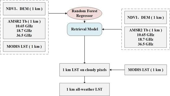
3.2. RF-Based LST Estimation

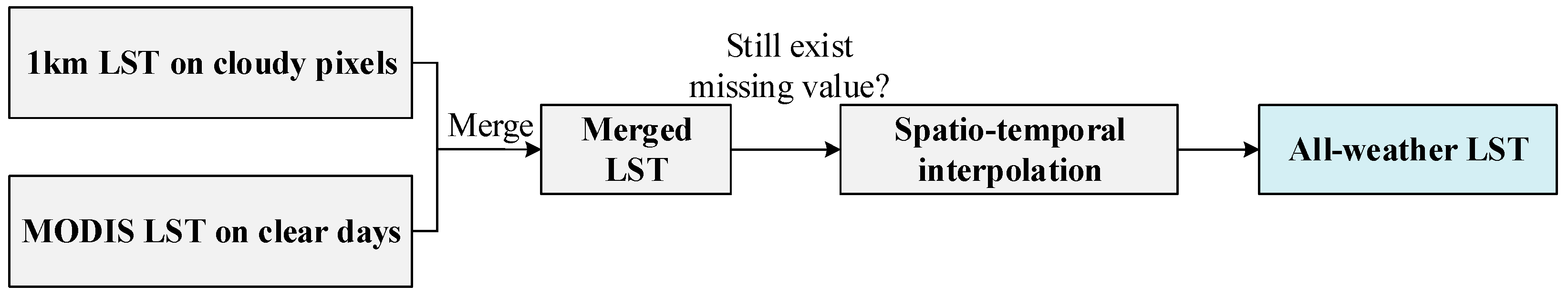
The spatial and temporal dynamics of LST are very complex since they depend on a variety of land surface variables, such as land cover and topography. The v-pol brightness temperature has been shown to be more sensitive to LST than the h-pol brightness temperature [44]. In addition, the 37 GHz v-pol brightness temperature shows a good linear relationship with LST and is thus considered the best microwave band for LST retrieval. However, it is not ideal to retrieve LST using 37 GHz v-pol brightness temperature in sparse and open shrubs because the brightness temperature in 37 GHz is affected by vegetation and soil water [24]. To identify the best variables for the RF regression, we created different groups of variables using 10.65 GHz,18.7 GHz and 36.5 GHz v-pol brightness temperatures. Each group also included DEM and NDVI, and half of them also included the microwave polarization difference index (MPDI). For each group, we performed 10-fold cross-validation, and the error was evaluated using the root mean square error (RMSE;

Table 3. The groups of variables used in the random forest-based LST estimation and their RMSE.

	Band	without MPDI	with MPDI	Band	without MPDI	with MPDI	Band	without MPDI	with MPDI
Single band	10.65 GHz	4.91 K	2.67 K	18.7 GHz	5.00 K	2.66 K	36.5 GHz	5.17 K	2.69 K
Two bands	10.65 GHz	2.64 K	2.71 K	10.65 GHz	2.66 K	2.71 K	18.7 GHz	2.66 K	2.70 K
	18.7 GHz			36.5 GHz			36.5 GHz
Three bands	10.65 GHz	2.62 K	2.71 K
	18.7 GHz
	36.5 GHz

). The plot of feature importance shows that the 37 GHz v-pol brightness temperature is of the highest importance and plays a leading role in LST retrieval (Figure 3). The second most important variable is DEM, which describes the influence of topography on the LST in the Tibetan Plateau. We found that when the number of estimators is 131 and the max depth is 39, the RF yields the smallest RMSE. Consequently, the 36.5 GHz v-pol brightness temperature was used to constrain the range of LST, and the 10.65 GHz and 18.7 GHz v-pol brightness temperature were used to correct the effects of vegetation and soil moisture.

RF has been widely used in classification and nonlinear regression problems in remote sensing [51,52]. RF is robust to outliers and to unbalanced data, ensuring efficient performance. The proposed RF method is based on the statistical relationship between LST and auxiliary variables and involves the following two phases (Figure 4): (1) training and (2) prediction. During training, we ensured that the brightness temperature, MODIS LST, NDVI and DEM had the same spatial resolution and that pixels acquired under clear-sky conditions were used to train the retrieval model with both ascending and descending acquisition. In the prediction phase, the model built through training was applied to the resampled brightness temperature and other auxiliary data to predict the 1 km LST for cloudy pixels.

At present, there are two ways to retrieve high-resolution LST from passive microwave brightness temperature, namely, inversion–disaggregation and disaggregation–inversion. The first way uses the brightness temperature to retrieve low-resolution LST, then downscales the LST to a high resolution. The second way disaggregates the brightness temperature to a MODIS resolution, then uses the resampled brightness temperature to retrieve high-resolution LST. It should be noted that the process of retrieving LST from AMSR2 introduces great uncertainty, which is inherited by the downscaled results. Therefore, we compared these two methods at a 10 km resolution. First, we trained the RF model at a 10 km resolution and estimated the 10 km LST. Then, the 1 km resolution LST estimated by the RF disaggregation–inversion method was aggregated to the resolution of AMSR2. Finally, we calculated r and RMSE between the estimated 10 km LST and MODIS LST. As shown in Figure 5, the second method had smaller errors; thus, disaggregation–inversion was chosen in the present study.

3.3. LST Fusion

The 1 km LST estimated can be merged directly with MODIS LST. After the fusion of 1 km LST for cloudy pixels and MODIS LST, some areas still had missing data because of the AMSR2 scanning gaps. In this study, we first used a temporally neighboring interpolation, and then used a spatially neighboring interpolation to supplement the gap. Because the gap is particularly wide at low latitudes, we were unable to obtain an acceptable error if we used spatially neighboring interpolation directly. Temporally neighboring interpolation assumed that the cloud coverage was the same on adjacent days, and used the LST of the day before and after to interpolate the LST of a given date. If the data was still missing after the temporally neighboring interpolation, spatially neighboring interpolation was performed. The procedure for the estimation method of 1 km LST is shown in Figure 6.

Inverse distance weighting (IDW), regular kriging (Kriging) and regular spline function (Spline) are three widely used spatial interpolation methods. To find better spatially neighboring interpolation methods, the errors of three spatial interpolation methods in different land use types of the Tibetan Plateau were compared. Firstly, we used land cover products as criteria to obtain MODIS LST data under every land cover type. Secondly, we assumed the same cloud coverage area for every land cover type, and used three spatial interpolation methods to estimate the LST value under the assumed cloud coverage area. Finally, we calculated the RMSE between the estimated LST and original LST (Figure 7). For urban, cropland, water, forest, bare land and grass, Spline had the smallest error. For snow/ice, Kriging had the smallest error. As Spline interpolation had, in general, smaller errors (0.10–2.73 K) under different land use/covers, it was selected.

3.4. Algorithm Evaluation Strategy

Because the LST retrieved by AMSR2 has a large uncertainty, it is necessary to evaluate its error to better evaluate the RF algorithm used in this paper, using r and RMSE as performance metrics. The AMSR2 LST under clear-sky pixels was compared to MODIS LST and in situ soil temperature. The AMSR2 LST under cloudy sky pixels was only compared to soil temperature because there was no MODIS LST for cloudy sky pixels. In addition, we chose the ST dataset from the GEOS-5 FP products as the reference to evaluate the RF method in this paper using the methods of Holmes, Zhao, and Zeng [24,44,53]. Since the datasets are spatially inconsistent (0.3125° by 0.25° for GEOS-5 ST, 1 km for the RF method, 10 km for the other three methods), the estimated LST was resampled to 0.25° by 0.25° by using the nearest-neighbor interpolation method, which is a feasible sampling approach and is extensively adopted in existing validation studies [54,55,56,57].

Holmes et al. (2009) developed a simple linear relationship of 37 GHz v-pol brightness temperature to obtain LST. The deviation of this method is within 1 K for 70% of the vegetated pixels. Due to its simple expression, it has been widely used as a soil temperature retrieval algorithm and in corresponding research [58,59,60]. It can be expressed as:

$${T_s}^{MW}=1.11T_{b,37v}-15.2 for T_{b,37v}>259.8$$

(3)

where T_b,37v is the brightness temperature of 36.5 GHz v-pol.

Zeng et al. (2014) established the LST inversion model in the Tibetan Plateau using ascending and descending AMSR-E brightness temperature. It can be expressed with Equations (4) and (5):

$$T_s=0.6885T_{B,36.5V\left[dsc\right]}+99.219$$

(4)

$$T_s=0.7664T_{B,36.5V\left[asc\right]}+72.206$$

(5)

where Ts denotes LST, and T_B,36.5V[dsc], T_B,36.5V[asc] respectively represent the brightness temperature of 36.5 GHz V-pol of AMSR-E in descending and ascending modes.

Zhao et al. (2011) established the LST inversion model in the Tibetan Plateau using AMSR-E brightness temperature and soil temperature. The minimum RMSE was 3.8046 K. It can be expressed as Equation (6). We found that there is 4-digit precision in coefficient values of Equation (6). To assess whether 4-digit precision is necessary, we have conducted an additional experiment; the experiment is based on the MODIS LST and AMSR2 brightness temperature. Firstly, we used 4-digit, 3-digit, 2-digit and 1-digit coefficients to estimate the 10 km LST. Then, we resampled the 1 km MODIS LST into 10 km. Finally, we calculated the correlation coefficients (R) and RMSE between the estimated LST and MODIS LST. The RMSE value of 3-digit coefficients increased by 0.02 K compared with the 4-digit coefficients, which clearly showed that 4-digit precision in coefficients is necessary.

$$\begin{array}{cc}\hfill T_S=& -0.0764T_{Bv}\left(10.65\right)+12.6656\mathrm{M}\mathrm{P}\mathrm{D}\mathrm{I}\left(10.65\right)\hfill \\ \hfill & +1.0312T_{Bv}\left(18.7\right)-22.6005\mathrm{M}\mathrm{P}\mathrm{D}\mathrm{I}\left(18.7\right)\hfill \\ \hfill & -0.2835T_{Bv}\left(36.5\right)+10.6500\mathrm{M}\mathrm{P}\mathrm{D}\mathrm{I}\left(36.5\right)+89.3601\hfill \end{array}$$

(6)

where T_Bv denotes the brightness temperature at the corresponding frequency. MPDI can be expressed with Equation (7), where a is 100 and f denotes frequency:

$$\mathrm{MPDI}\left(\mathrm{f}\right)=\mathrm{a}·\left[T_{Bv}\left(\mathrm{f}\right)-T_{Bh}\left(\mathrm{f}\right)]/[T_{Bv}\left(\mathrm{f}\right)+T_{Bh}\left(\mathrm{f}\right)\right]$$

(7)

There are a lot of alternatives to random forest; to make sure that the choice of random forest is justified, we made a comparison between the classic MLR-based methodology and regression techniques in machine learning (neural networks, nearest neighbor, ensembles such as random forests). The evaluated algorithms included MLR (multiple linear regression), MLP (multilayer perceptron), CART (Classification and Regression Tree), KNR (K-nearest neighbor regression), GBRT (gradient boost regression tree) and RF (random forest). These are representative regression models; however, few studies have been conducted to compare their quality in predicting LST [38,61,62]. For each model, we did 10-fold cross-validation to find the optimized parameters. Then, we calculated the R² and RMSE of each model under the optimized parameters.

4. Results and Discussion

4.1. LST Maps

Figure 8 shows the original MODIS LST (first row) and the all-weather 1 km LST (second row) over the Tibetan Plateau from May 2015 to April 2016. The original MODIS LST had some missing data due to cloud contamination, and was thus spatio-temporally discontinuous. Compared with the original MODIS LST, the results are spatio-temporally continuous. Spatially, the LST on the second row continues the spatial variation trend of the original MODIS LST. The LST decreases from southeast to northwest, which is consistent with the terrain of the Tibetan Plateau, which is higher in the northwest and lower in the southeast. Temporally, the all-weather 1 km LST captures well the monthly variation of temperature in the Tibetan Plateau, with a higher LST in summer (from June to August).

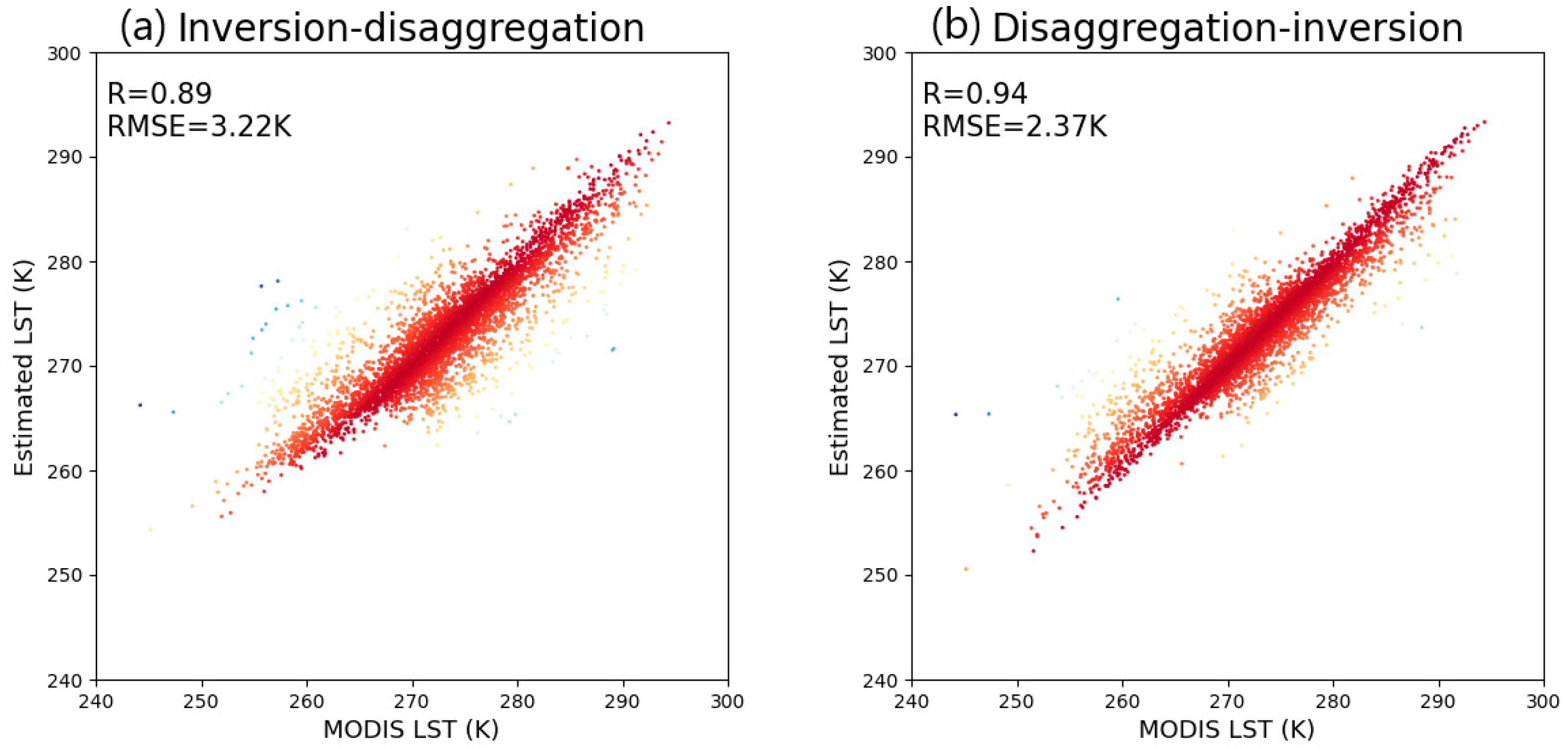
4.2. Different Methods Comparison

Based on the descending orbit data of 2 June 2015, we calculated the probability density histogram of the difference between the estimated LST and GEOS-5 LST (Figure 9). The distribution of the difference is close to the normal distribution for each method. The expectations ($\mu$) for Holmes, Zhao, and our method are less than zero, which indicates an underestimation. In contrast, the $\mu$ of the Zeng method is 5.28, which indicates an overestimation. In addition, the $\mu$ of the Holmes method ($\mu =-2.23$) and the method in this paper ($\mu =-2.84$) are closer to zero. In terms of standard deviation ($\sigma$), the method in this paper yields the smallest $\sigma$ of 6.19, which shows that the errors are more centralized. In conclusion, compared with other methods, the method in this paper yields better expectation and standard deviation, with a difference that is more centralized around zero.

We calculated the r and RMSE between the estimated LST/MODIS LST and GEOS-5 LST. As shown in Figure 10, the Holmes method yields the worst result (r = 0.66 and RMSE = 12.48 K). This was followed by the Zhao method, which had an r of 0.33 and an RMSE of 12.15 K. The Holmes method and the Zeng method have the same r (0.66); the Zeng method has a smaller RMSE (8.89 K), indicating that the Zeng method performs better—perhaps because it is an improvement of the Holmes method. As the Zeng method is based on the 0–5 cm in situ soil temperature data from the Tibetan Plateau, it may be more suitable for the Tibetan Plateau. In conclusion, the RMSE values of the Holmes and the Zeng methods are both large: 12.48 K and 8.89 K, respectively. The r and RMSE of the method in this paper are 0.5 and 6.81 K; the error is close to that of the MODIS LST, showing that the RF method predicts LST with the smallest error compared with other methods. This could be because the RF method in this paper used the MODIS LST for training and therefore the LST it predicted was more similar to the GEOS-5 LST; in contrast, other methods used ground measurements as the true values.

Table 4. Comparison between the classic MLR-based methodology and regression techniques imachine learning.

Models	Optimized Parameters	R2	RMSE, K	Training Time
MLR	NA	0.44	5.39	0:00:08
MLP	1 hidden layer with 2000 neurons	0.63	4.39	12:08:58
CART	Max_depth = 16	0.66	4.22	0:10:34
KNR	N_neighbors = 5	0.74	3.67	0:12:14
GBRT	N_estimators = 282 Max_depth = 18	0.79	3.26	21:36:33
RF	N_estimators = 131 Max_depth = 39	0.81	3.17	0:14:38

MLR (multiple linear regression), MLP (multilayer perceptron), CART (classification and regression tree), KNR (K-neighbor regressor), GBRT (gradient boost regression tree), RF (random forest).

is the comparison between the classic MLR-based methodology and regression techniques in machine learning. The results confirm that classic MLR is outperformed by machine learning techniques and concretely, our experiments suggest that random forest regression outperforms the rest of the techniques.

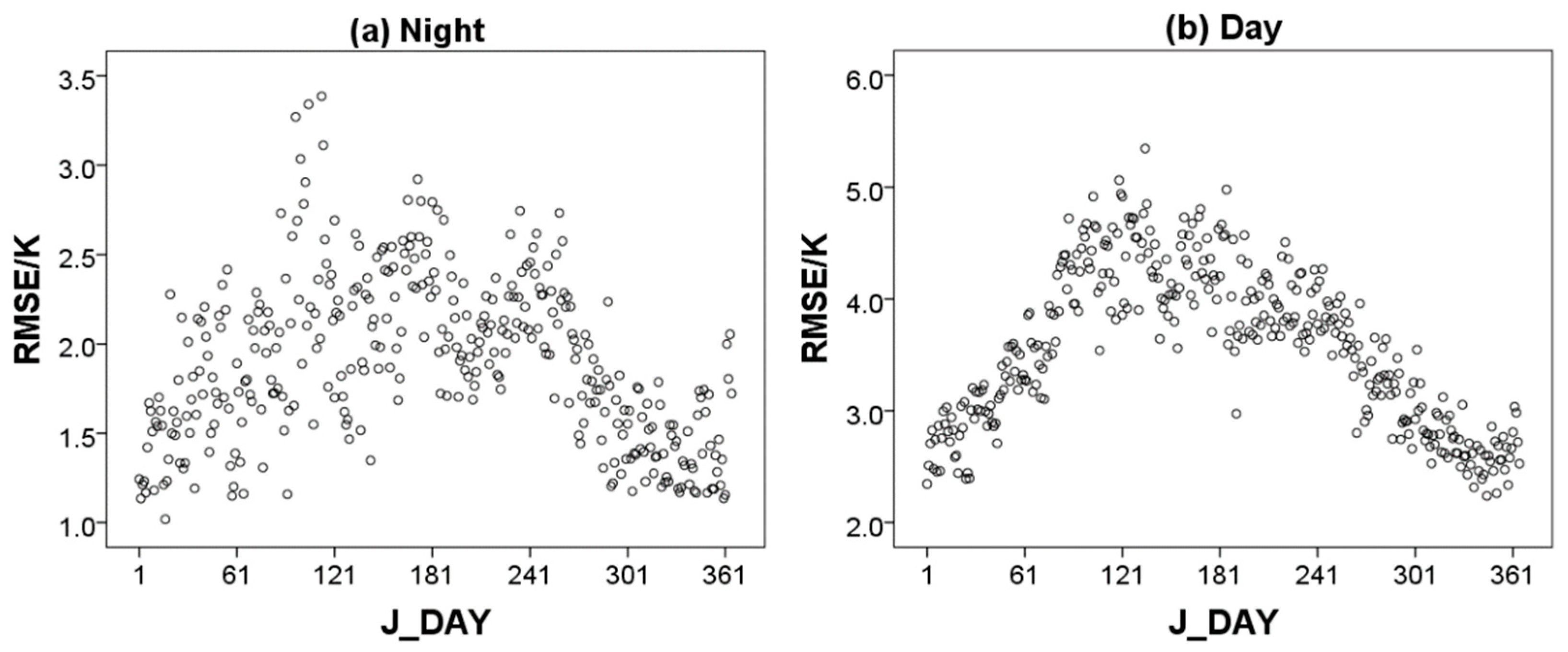
4.3. Evaluation Using MODIS LST

Since MODIS LST products have been evaluated to have an error of less than 1 K at most areas, the AMSR2 LST predicted by RF were compared with the MODIS LST for validation using r and RMSE as performance metrics. We selected the dates of 1 July 2015, 1 October 2015, 1 January 2016 and 1 April 2016 to represent the summer, autumn, winter, and spring of the Tibetan Plateau, respectively. Figure 11 shows the scatter plot of predicted LST and MODIS LST. At night-time, the r was between 0.92 and 0.97, and the RMSE was between 1.16 K and 2.4 K. At daytime, the r was between 0.9 and 0.93, and the RMSE was between 2.35 K and 4.67 K. This shows that the night-time error is smaller than that of the daytime. This may be because the spatial heterogeneity of LST at night is smaller than that during the day, so the relationship between the LST and its predictors (NDVI, DEM, AMSR2 BT) is simpler and the RF model we obtain is more accurate. The figure also shows that the prediction error is smaller in autumn, winter, and spring than that in summer. The reason may be that there is more rainfall in summer, and the microwave signal is interfered with by the water vapor in the atmosphere, so the radiation transmission process is more complex.

To understand the error for the entire year, we calculated the r and RMSE between the predicted LST and MODIS LST for every day and night from 1 May 2015 to 30 April 2016. The predicted LST at night has a higher correlation with the MODIS LST (Figure 12). During the night-time, most r values are close to 0.94. During the daytime, most r values are close to 0.92. The predicted LST at night has a smaller RMSE with the MODIS LST (Figure 13). During the nighttime, the RMSE is in the range between 1.02 K and 3.39 K. During the daytime, the RMSE is in the range between 2.24 K and 5.35 K. The r and RMSE values can be compared with the r and RMSE values of previous machine learning methods. The ANN method Shwetha used to predict high spatio-temporal resolution land surface temperatures under cloudy conditions shows r values from 0.56 to 0.90 and RMSE values from 1.70 K to 2.12 K during the night-time, and has r values from 0.78 to 0.96 and RMSE values from 1.86 K to 4.00 K during the daytime [38]. Overall, there is a significant r and a small RMSE between the predicted LST and the MODIS LST both during the day and at night, indicating the ability of RF in predicting the LST.

4.4. Evaluation Using In Situ Measurements

The LST estimated by AMSR2 brightness temperature and RF was validated with a 0–5 cm soil temperature. The soil temperature was measured by a high-precision temperature measuring instrument. According to the station screening rules mentioned in the data preprocessing, the in situ soil surface temperature reasonably represents the 1 km LST in this study because these stations have an acceptable spatial heterogeneity. The stations are PL01, PL03, PL05, PL11, PL12, AL02 and SQ16. Figure 14 shows the scatter plot between the estimated LST and the in situ soil surface temperature. The estimated LST is close to the in situ surface temperature, and the RMSE is from 5.60 K to 10.56 K.

The retrieved AMSR2 LST under clear and cloudy conditions were respectively compared with the in-situ soil temperature. There is a scale difference between the in situ soil temperature and the 1 km LST, so the error caused by scale mismatch should be measured. Because the MODIS LST products have been verified to have an error of less than 1 K, this paper calculated the RMSE between the MODIS LST and in situ soil temperature to represent the error caused by the scale mismatch. Figure 15 shows the scatter plot between the in situ soil temperature and MODIS LST, and the AMSR2 LST under clear and cloudy conditions. Compared to the MODIS LST, the LST retrieved by RF is closer to the in-situ soil temperature. The retrieved LST under cloudy skies is closer to the in situ soil temperature than that under clear skies.

The r and RMSE between the remote sensing LST and in situ soil temperature were calculated for each in situ station for both clear and cloudy sky pixels (

Table 5. R and RMSE between predicted LST and soil temperature.

Site	Clear-Sky				Cloud-Sky
	LST_MODIS/Ta		LST_AMSR2/Ta		LST_AMSR2/Ta
	R	RMSE/K	R	RMSE/K	R	RMSE/K
PL01	0.715	8.451	0.661	6.139	0.654	5.152
PL03	0.731	10.585	0.54	8.775	0.574	6.804
PL05	0.676	11.34	0.385	9.475	0.678	6.635
PL11	0.81	8.923	0.776	7.574	0.674	5.825
PL12	0.324	7.921	0.463	6.754	0.324	6.579
AL02	0.926	5.398	0.908	5.132	0.649	6.995
SQ16	0.611	13.143	0.649	12.349	0.745	5.429

). For MODIS LST under clear-sky pixels, r ranged from 0.324 (PL12) to 0.926 (AL02) and RMSE ranged from 5.398 K (AL02) to 13.143 K (SQ16). For the AMSR2 LST under a clear sky, r ranged from 0.385 (PL05) to 0.908 (AL02) and RMSE ranged from 5.132 K (AL02) to 12.349 K (SQ16). For the AMSR2 LST under a cloudy sky, the r ranged from 0.324 (PL12) to 0.745 (SQ16) and the RMSE ranged from 5.152 K (PL01) to 6.995 K (AL02). Overall, Table 5 indicates that the estimated AMSR2 LST has a similar error as the MODIS LST. In addition, the RMSE of the AMSR2 LST under a cloudy sky is similar with that under a clear sky—this shows that RF can yield the same satisfactory accuracy under a cloudy sky as under a clear sky. The RMSE of the AMSR2 LST under a cloudy sky (5.152–6.995 K) is comparable to the RMSE of the ANN method proposed by Shwetha (2.9 K to 6.2 K for a cloudy sky) [38].

5. Conclusions

In this paper, a machine learning method was proposed to estimate all-weather 1 km LST over the Tibetan Plateau. The method resampled the brightness temperature of AMSR2 into a 1 km resolution, then used RF regression to define a nonlinear relationship between MODIS LST and surface variables to estimate the 1 km LST under cloudy skies. Following LST fusion and interpolation, all-weather 1 km LST data was generated.

In situ measurements and MODIS LST were used to evaluate the algorithm. The results show that the LST predicted by RF is consistent with the MODIS LST and 0–5 cm soil temperature. Additionally, the method fills the gaps caused by cloud cover, which can lead to incomplete data over a large area. The gap-filled LST captures the spatiotemporal variation trend of MODIS LST. This method makes it possible to obtain all-weather 1 km LST datasets, which can support regional and even global climate change research. Nevertheless, there is still room for further improvement of the method regarding the following aspects: (1) an AMSR2-derived LST downscaling method should be developed; downscaling is an important research topic that was simplified for this paper. State-of-the-art downscaling approaches should be further explored; (2) a more accurate time interpolation method is needed, which may use meteorological or other satellite data to decrease errors; (3) although this study has focused on the Tibetan Plateau, we believe that this method could be used over other regions—but additional validation will be needed.

References

1. Coll, C.; García-Santos, V.; Niclos, R.; Caselles, V. Test of the MODIS land surface temperature and emissivity separation algorithm with ground measurements over a rice paddy. IEEE Trans. Geosci. Remote Sens. 2016, 54, 3061–3069. [Google Scholar] [CrossRef]
2. Wan, Z.; Li, Z.L. A physics-based algorithm for retrieving land-surface emissivity and temperature from EOS/MODIS data. IEEE Trans. Geosci. Remote Sens. 1997, 35, 980–996. [Google Scholar]
3. Duan, S.B.; Li, Z.L.; Tang, B.H.; Wu, H.; Tang, R. Generation of a time-consistent land surface temperature product from MODIS data. Remote Sens. Environ. 2014, 140, 339–349. [Google Scholar] [CrossRef]
4. Xia, H.; Chen, Y.; Li, Y.; Quan, J. Combining kernel-driven and fusion-based methods to generate daily high-spatial-resolution land surface temperatures. Remote Sens. Environ. 2019, 224, 259–274. [Google Scholar] [CrossRef]
5. Haashemi, S.; Weng, Q.; Darvishi, A.; Alavipanah, S.K. Seasonal variations of the surface urban heat island in a semi-arid city. Remote Sens. 2016, 8, 352. [Google Scholar] [CrossRef] [Green Version]
6. Mirzaei, M.; Verrelst, J.; Arbabi, M.; Shaklabadi, Z.; Lotfizadeh, M. Urban heat island monitoring and impacts on citizen’s general health status in Isfahan metropolis: A remote sensing and field survey approach. Remote Sens. 2020, 12, 1350. [Google Scholar] [CrossRef]
7. Imhoff, M.L.; Zhang, P.; Wolfe, R.E.; Bounoua, L. Remote sensing of the urban heat island effect across biomes in the continental USA-ScienceDirect. Remote Sens. Environ. 2010, 114, 504–513. [Google Scholar] [CrossRef] [Green Version]
8. Maimaitiyiming, M.; Ghulam, A.; Tiyip, T.; Pla, F.; Latorre-Carmona, P.; Halik, Ü.; Caetano, M. Effects of green space spatial pattern on land surface temperature: Implications for sustainable urban planning and climate change adaptation. ISPRS J. Photogramm. Remote Sens. 2014, 89, 59–66. [Google Scholar] [CrossRef] [Green Version]
9. Rhee, J.; Im, J.; Carbone, G.J. Monitoring agricultural drought for arid and humid regions using multi-sensor remote sensing data. Remote Sens. Environ. 2010, 114, 2875–2887. [Google Scholar] [CrossRef]
10. Rousta, I.; Olafsson, H.; Moniruzzaman, M.; Zhang, H.; Liou, Y.A.; Mushore, T.D.; Gupta, A. Impacts of Drought on Vegetation Assessed by Vegetation Indices and Meteorological Factors in Afghanistan. Remote Sens. 2020, 12, 2433. [Google Scholar] [CrossRef]
11. Hu, T.; Renzullo, L.J.; van Dijk, A.I.; He, J.; Tian, S.; Xu, Z.; Zhou, J.; Liu, T.; Liu, Q. Monitoring agricultural drought in Australia using MTSAT-2 land surface temperature retrievals. Remote Sens. Environ. 2020, 236, 111419. [Google Scholar] [CrossRef]
12. Yang, M.; Zhao, W.; Zhan, Q.; Xiong, D. Spatiotemporal patterns of land surface temperature change in the tibetan plateau based on MODIS/Terra daily product from 2000 to 2018. IEEE J. Sel. Top. Appl. Earth Obs. Remote Sens. 2021, 14, 6501–6514. [Google Scholar] [CrossRef]
13. Tan, J.; Yu, D.; Li, Q.; Tan, X.; Zhou, W. Spatial relationship between land-use/land-cover change and land surface temperature in the Dongting Lake area, China. Sci. Rep. 2020, 10, 1–9. [Google Scholar] [CrossRef]
14. Wang, L.; Koike, T.; Yang, K.; Yeh, P.J. Assessment of a distributed biosphere hydrological model against streamflow and MODIS land surface temperature in the upper Tone River Basin. J. Hydrol. 2009, 377, 21–34. [Google Scholar] [CrossRef]
15. Parinussa, R.M.; Lakshmi, V.; Johnson, F.; Sharma, A. Comparing and combining remotely sensed land surface temperature products for improved hydrological applications. Remote Sens. 2016, 8, 162. [Google Scholar] [CrossRef] [Green Version]
16. Renzullo, L.J.; Barrett, D.J.; Marks, A.S.; Hill, M.J.; Guerschman, J.P.; Mu, Q.; Running, S.W. Multi-sensor model-data fusion for estimation of hydrologic and energy flux parameters. Remote Sens. Environ. 2008, 112, 1306–1319. [Google Scholar] [CrossRef]
17. Holzman, M.E.; Rivas, R.; Piccolo, M.C. Estimating soil moisture and the relationship with crop yield using surface temperature and vegetation index. Int. J. Appl. Earth Obs. Geoinf. 2014, 28, 181–192. [Google Scholar] [CrossRef]
18. Anderson, M.C.; Zolin, C.A.; Sentelhas, P.C.; Hain, C.R.; Semmens, K.; Yilmaz, M.T.; Gao, F.; Otkin, J.A.; Tetrault, R. The Evaporative Stress Index as an indicator of agricultural drought in Brazil: An assessment based on crop yield impacts. Remote Sens. Environ. 2016, 174, 82–99. [Google Scholar] [CrossRef]
19. Jimenez-Munoz, J.C.; Sobrino, J.A. A single-channel algorithm for land surface temperature retrieval from ASTER data. IEEE Geosci. Remote Sens. Lett. 2010, 7, 176–179. [Google Scholar] [CrossRef]
20. Becker, F.; Li, Z.L. Towards a local split window method over land surfaces. Int. J. Remote Sens. 1990, 11, 369–393. [Google Scholar] [CrossRef]
21. Li, Z.L.; Tang, B.H.; Wu, H.; Ren, H.; Yan, G.; Wan, Z.; Trigo, I.F.; Sobrino, J.A. Satellite-derived land surface temperature: Current status and perspectives. Remote Sens. Environ. 2013, 131, 14–37. [Google Scholar] [CrossRef] [Green Version]
22. Li, Z.L.; Wu, H.; Wang, N.; Qiu, S.; Sobrino, J.A.; Wan, Z.; Tang, B.H.; Yan, G. Land surface emissivity retrieval from satellite data. Int. J. Remote Sens. 2013, 34, 3084–3127. [Google Scholar] [CrossRef]
23. Martins, J.; Trigo, I.F.; Ghilain, N.; Jimenez, C.; Göttsche, F.M.; Ermida, S.L.; Olesen, F.S.; Gellens-Meulenberghs, F.; Arboleda, A. An all-weather land surface temperature product based on MSG/SEVIRI observations. Remote Sens. 2019, 11, 3044. [Google Scholar] [CrossRef] [Green Version]
24. Holmes, T.R.H.; De Jeu, R.A.M.; Owe, M.; Dolman, A.J. Land surface temperature from Ka band (37 GHz) passive microwave observations. J. Geophys. Res. Atmos. 2009, 114, D04113. [Google Scholar] [CrossRef] [Green Version]
25. Fily, M.; Royer, A.; Goıta, K.; Prigent, C. A simple retrieval method for land surface temperature and fraction of water surface determination from satellite microwave brightness temperatures in sub-arctic areas. Remote Sens. Environ. 2003, 85, 328–338. [Google Scholar] [CrossRef]
26. Prigent, C.; Rossow, W.R. Retrieval of surface and atmospheric parameters over land from SSM/I: Potential and limitations. Q. J. R. Meteorol. Soc. 1999, 125, 2379–2400. [Google Scholar] [CrossRef]
27. Jin, M.; Dickinson, R.E. A generalized algorithm for retrieving cloudy sky skin temperature from satellite thermal infrared radiances. J. Geophys. Res. Atmos. 2000, 105, 27037–27047. [Google Scholar] [CrossRef]
28. Lu, L.; Venus, V.; Skidmore, A.; Wang, T.; Luo, G. Estimating land-surface temperature under clouds using MSG/SEVIRI observations. Int. J. Appl. Earth Obs. Geoinf. 2011, 13, 265–276. [Google Scholar] [CrossRef]
29. Hengl, T.; Heuvelink, G.B.; Tadić, M.P.; Pebesma, E.J. Spatio-temporal prediction of daily temperatures using time-series of MODIS LST images. Theor. Appl. Climatol. 2012, 107, 265–277. [Google Scholar] [CrossRef] [Green Version]
30. Xu, S.; Cheng, J.; Zhang, Q. A Random Forest-Based Data Fusion Method for Obtaining All-Weather Land Surface Temperature with High Spatial Resolution. Remote Sens. 2021, 13, 2211. [Google Scholar] [CrossRef]
31. Yoo, C.; Im, J.; Cho, D.; Yokoya, N.; Xia, J.; Bechtel, B. Estimation of all-weather 1 km MODIS land surface temperature for humid summer days. Remote Sens. 2020, 12, 1398. [Google Scholar] [CrossRef]
32. Long, D.; Yan, L.; Bai, L.; Zhang, C.; Li, X.; Lei, H.; Yang, H.; Tian, F.; Zeng, C.; Meng, X.; et al. Generation of MODIS-like land surface temperatures under all-weather conditions based on a data fusion approach. Remote Sens. Environ. 2020, 246, 111863. [Google Scholar] [CrossRef]
33. Zhang, X.; Zhou, J.; Liang, S.; Wang, D. A practical reanalysis data and thermal infrared remote sensing data merging (RTM) method for reconstruction of a 1-km all-weather land surface temperature. Remote Sens. Environ. 2021, 260, 112437. [Google Scholar] [CrossRef]
34. Xu, S.; Cheng, J. A new land surface temperature fusion strategy based on cumulative distribution function matching and multiresolution Kalman filtering. Remote Sens. Environ. 2021, 254, 112256. [Google Scholar] [CrossRef]
35. Zhang, X.; Zhou, J.; Dong, W.; Song, L. Estimation of 1-Km All-Weather Land Surface Temperature Over the Tibetan Plateau. In Proceedings of the IGARSS 2018—2018 IEEE International Geoscience and Remote Sensing Symposium, Valencia, Spain, 22–27 July 2018; pp. 3430–3433. [Google Scholar]
36. Gao, Z.; Hou, Y.; Zaitchik, B.F.; Chen, Y.; Chen, W. A Two-Step Integrated MLP-GTWR Method to Estimate 1 km Land Surface Temperature with Complete Spatial Coverage in Humid, Cloudy Regions. Remote Sens. 2021, 13, 971. [Google Scholar] [CrossRef]
37. Duan, S.B.; Li, Z.L.; Leng, P.; Han, X.J.; Chen, Y. Generation of an all-weather land surface temperature product from MODIS and AMSR-E data. In Proceedings of the International Conference on Intelligent Earth Observing and Applications, Guilin, China, 9 December 2015; pp. 1–5. [Google Scholar]
38. Shwetha, H.R.; Kumar, D.N. Prediction of high spatio-temporal resolution land surface temperature under cloudy conditions using microwave vegetation index and ANN. ISPRS J. Photogramm. Remote Sens. 2016, 117, 40–55. [Google Scholar] [CrossRef]
39. Li, A.; Bo, Y.; Zhu, Y.; Guo, P.; Bi, J.; He, Y. Blending multi-resolution satellite sea surface temperature (SST) products using Bayesian Maximum Entropy method. Remote Sens. Environ. 2013, 135, 52–63. [Google Scholar] [CrossRef]
40. Kou, X.; Jiang, L.; Bo, Y.; Yan, S.; Chai, L. Estimation of land surface temperature through blending MODIS and AMSR-E Data with the Bayesian Maximum Entropy method. Remote Sens. 2016, 8, 105. [Google Scholar] [CrossRef] [Green Version]
41. Duan, S.; Li, Z.; Leng, P. A framework for the retrieval of all-weather land surface temperature at a high spatial resolution from polar-orbiting thermal infrared and passive microwave data. Remote Sens. Environ. 2017, 195, 107–117. [Google Scholar] [CrossRef]
42. Zhang, X.; Zhou, J.; Liang, S.; Chai, L.; Wang, D.; Liu, J. Estimation of 1-km all-weather remotely sensed land surface temperature based on reconstructed spatial-seamless satellite passive microwave brightness temperature and thermal infrared data. ISPRS J. Photogramm. Remote Sens. 2020, 167, 321–344. [Google Scholar] [CrossRef]
43. Yu, J.; Zhang, G.; Yao, T.; Xie, H.; Zhang, H.; Ke, C.; Yao, R. Developing Daily Cloud-Free Snow Composite Products from MODIS Terra–Aqua and IMS for the Tibetan Plateau. IEEE Trans. Geo Sci. Remote Sens. 2016, 54, 2171–2180. [Google Scholar] [CrossRef]
44. Zhao, T.J.; Zhang, L.X.; Shi, J.C.; Jiang, L.M. A physically based statistical methodology for surface soil moisture retrieval in the Tibet Plateau using microwave vegetation indices. J. Geophys. Res. Atmos. 2011, 116. [Google Scholar] [CrossRef]
45. Chen, S.S.; Chen, X.Z.; Chen, W.Q.; Su, Y.X.; Li, D. A simple retrieval method of land surface temperature from AMSR-E passive microwave data—A case study over Southern China during the strong snow disaster of 2008. Int. J. Appl. Earth Obs. Geoinf. 2011, 13, 140–151. [Google Scholar] [CrossRef]
46. Zabolotskikh, E.V.; Mitnik, L.M.; Reul, N.; Chapron, B. New possibilities for geophysical parameter retrievals opened by GCOM-W1 AMSR2. IEEE J. Sel. Top. Appl. Earth Obs. Remote Sens. 2015, 8, 4248–4261. [Google Scholar] [CrossRef]
47. Imaoka, K.; Kachi, M.; Fujii, H.; Murakami, H.; Hori, M.; Ono, A.; Igarashi, T.; Nakagawa, K.; Oki, T.; Honda, Y.; et al. Global Change Observation Mission (GCOM) for monitoring carbon, water cycles, and climate change. Proc. IEEE 2010, 98, 717–734. [Google Scholar] [CrossRef]
48. Ma, H.; Zeng, J.; Zhang, X.; Fu, P.; Zheng, D.; Wigneron, J.P.; Chen, N.; Niyogi, D. Evaluation of six satellite-and model-based surface soil temperature datasets using global ground-based observations. Remote Sens. Environ. 2021, 264, 112605. [Google Scholar] [CrossRef]
49. Wilheit, T.; Kummerow, C.D.; Ferraro, R. NASDARainfall algorithms for AMSR-E. IEEE Trans. Geosci. Remote Sens. 2003, 41, 204–214. [Google Scholar] [CrossRef]
50. Pan, M.; Sahoo, A.K.; Wood, E.F. Improving soil moisture retrievals from a physically-based radiative transfer model. Remote Sens. Environ. 2014, 140, 130–140. [Google Scholar] [CrossRef]
51. Zhao, W.; Sánchez, N.; Lu, H.; Li, A. A spatial downscaling approach for the SMAP passive surface soil moisture product using random forest regression. J. Hydrol. 2018, 563, 1009–1024. [Google Scholar] [CrossRef]
52. Zhao, W.; Duan, S.B.; Li, A.; Yin, G. A practical method for reducing terrain effect on land surface temperature using random forest regression. Remote Sens. Environ. 2019, 221, 635–649. [Google Scholar] [CrossRef]
53. Zeng, J. Research on Passive Microwave Retrieval of Soil Moisture in the Qinghai-Tibet Plateau; Chinese Academy of Sciences University: Beijing, China, 2015. [Google Scholar]
54. Al-Yaari, A.; Wigneron, J.-P.; Ducharne, A.; Kerr, Y.; de Rosnay, P.; de Jeu, R.; Govind, A.; al Bitar, A.; Albergel, C.; Munoz-Sabater, J. Global-scale evaluation of two satellite-based passive microwave soil moisture datasets (SMOS and AMSR-E) with respect to land data assimilation system estimates. Remote Sens. Environ. 2014, 149, 181–195. [Google Scholar] [CrossRef] [Green Version]
55. Cui, C.; Xu, J.; Zeng, J.; Chen, K.S.; Bai, X.; Lu, H.; Chen, Q.; Zhao, T. Soil moisture mapping from satellites: An Intercomparison of SMAP, SMOS, FY3B, AMSR2, and ESA CCI over two dense network regions at different spatial scales. Remote Sens. 2018, 10, 33. [Google Scholar] [CrossRef] [Green Version]
56. Zeng, J.; Li, Z.; Chen, Q.; Bi, H.; Qiu, J.; Zou, P. Evaluation of remotely sensed and reanalysis soil moisture products over the Tibetan plateau using in situ observations. Remote Sens. Environ. 2015, 163, 91–110. [Google Scholar] [CrossRef]
57. Ma, H.; Zeng, J.; Chen, N.; Zhang, X.; Cosh, M.H.; Wang, W. Satellite surface soil moisture from SMAP, SMOS, AMSR2 and ESA CCI: A comprehensive assessment using global ground-based observations. Remote Sens. Environ. 2019, 231, 111215. [Google Scholar] [CrossRef]
58. Dente, L.; Ferrazzoli, P.; Su, Z.; van der Velde, R.; Guerriero, L. Combined use of active and passive microwave satellite data to constrain a discrete scattering model. Remote Sens. Environ. 2014, 155, 222–238. [Google Scholar] [CrossRef]
59. Hong, S.; Shin, I. A physically-based inversion algorithm for retrieving soil moisture in passive microwave remote sensing. J. Hydrol. 2011, 405, 24–30. [Google Scholar] [CrossRef]
60. Liu, Q.; Du, J.; Shi, J.; Jiang, L. Analysis of spatial distribution and multi-year trend of the remotely sensed soil moisture on the Tibetan Plateau. Sci. China Earth Sci. 2013, 56, 2173–2185. [Google Scholar] [CrossRef]
61. García-Gutiérrez, J.; Martínez-Álvarez, F.; Troncoso, A.; Riquelme, J.C. A comparison of machine learning regression techniques for LiDAR-derived estimation of forest variables. Neurocomputing 2015, 167, 24–31. [Google Scholar] [CrossRef]
62. Chen, J.; de Hoogh, K.; Gulliver, J.; Hoffmann, B.; Hertel, O.; Ketzel, M.; Bauwelinck, M.; Van Donkelaar, A.; Hvidtfeldt, U.A.; Katsouyanni, K.; et al. A comparison of linear regression, regularization, and machine learning algorithms to develop Europe-wide spatial models of fine particles and nitrogen dioxide. Environ. Int. 2019, 130, 104934. [Google Scholar] [CrossRef] [PubMed]
Figure 1. Study area and soil temperature measurement sites. (a) DEM data were downloaded from the geospatial data cloud platform of the computer network information center of the Chinese Academy of Sciences. (b) AL02, SQ16, PL01, PL03, PL05, PL11, PL12 are the names of soil temperature sites, AL, SQ, PL represent different prefectures. (c) Land cover data were downloaded from the national Tibetan Plateau scientific data center.
Remotesensing 13 04574 g001
Figure 2. Coefficient of correlation (R) between brightness temperature (36.5 GHz) and MODIS LST. (a) before cubic interpolation. (b) after cubic interpolation. The darker color indicates a stronger correlation between two variables.
Remotesensing 13 04574 g002
Figure 3. The importance ranking of different variables used in the random forest-based LST estimation.
Remotesensing 13 04574 g003
Figure 4. Schematic diagram of the producer for estimating 1 km LST on cloudy pixels.
Remotesensing 13 04574 g004
Figure 5. The estimated LST compared to MODIS LST. (a) inversion-disaggregation. (b) disaggregation-inversion. The darker color indicates a stronger correlation between two variables.
Remotesensing 13 04574 g005
Figure 6. Procedure for merging estimated LST on cloudy pixels with MODIS LST.
Remotesensing 13 04574 g006
Figure 7. The RMSE of different spatial interpolation methods under different land use/covers.
Remotesensing 13 04574 g007
Figure 8. Monthly variation of the original MODIS LST and the all-weather 1 km LST of the Tibetan Plateau from May 2015 to April 2016. (a) May 2015. (b) June 2015. (c) July 2015. (d) August 2015. (e) September 2015. (f) October 2015. (g) November 2015. (h) December 2015. (i) January 2016. (j) February 2016. (k) March 2016. (l) April 2016.
Remotesensing 13 04574 g008
Figure 9. Probability density histogram of the difference between the estimated LST/MODIS LST and GEOS-5 LST. (a) Holmes method. (b) Zhao method. (c) Zeng method. (d) Method in this paper. (e) MODIS LST. In blue is the kernel density estimate (KDE); the red line represents the fitting standard normal distribution (norm).
Remotesensing 13 04574 g009
Figure 10. Coefficient of correlation (R) and root mean square error (RMSE) between the estimated LST by each method and GEOS-5 LST. (a) Holmes method. (b) Zhao method. (c) Zeng method. (d) Method in this paper. (e) MODIS LST. The darker color indicates a stronger correlation between two variables.
Remotesensing 13 04574 g010
Figure 11. Scatterplot of predicted LST and MODIS LST (a) 1 July 2015 night. (b) 1 July 2015 day. (c) 1 October 2015 night. (d) 1 October 2015 day. (e) 1 January 2016 night. (f) 1 January 2016 day. (g) 1 April 2016 night. (h) 1 April 2016 day. The darker color indicates a stronger correlation between two variables.
Remotesensing 13 04574 g011aRemotesensing 13 04574 g011b
Figure 12. R between the predicted LST and MODIS LST at night and daytime. (a) night. (b) day.
Remotesensing 13 04574 g012
Figure 13. RMSE between the predicted LST and MODIS LST at night and daytime. (a) night. (b) day.
Remotesensing 13 04574 g013
Figure 14. Comparison between estimated LST and in situ soil temperature at each site. (a) PL01. (b) PL03. (c) PL05. (d) PL11. (e) PL12. (f) AL02. (g) SQ16.
Remotesensing 13 04574 g014
Figure 15. Scatter plot between in situ soil temperature and LST_modis, and LST_AMSR2 under clear and cloudy conditions. (a) PL01. (b) PL03. (c) PL05. (d) PL11. (e) PL12. (f) AL02. (g) SQ16.
Remotesensing 13 04574 g015