
Mapping Forest Burn Extent from Hyperspatial Imagery Using Machine Learning


Department of Mathematics and Computer Science, Northwest Nazarene University, Nampa, ID 83686, USA
*
Author to whom correspondence should be addressed.
Remote Sens. 2021, 13(19), 3843; https://0-doi-org.brum.beds.ac.uk/10.3390/rs13193843
Submission received: 27 July 2021
/
Revised: 20 September 2021
/
Accepted: 22 September 2021
/
Published: 25 September 2021
(This article belongs to the Special Issue Remote Sensing of Burnt Area)
Abstract
:Support vector machines are shown to be highly effective in mapping burn extent from hyperspatial imagery in grasslands. Unfortunately, this pixel-based method is hampered in forested environments that have experienced low-intensity fires because unburned tree crowns obstruct the view of the surface vegetation. This obstruction causes surface fires to be misclassified as unburned. To account for misclassifying areas under tree crowns, trees surrounded by surface burn can be assumed to have been burned underneath. This effort used a mask region-based convolutional neural network (MR-CNN) and support vector machine (SVM) to determine trees and burned pixels in a post-fire forest. The output classifications of the MR-CNN and SVM were used to identify tree crowns in the image surrounded by burned surface vegetation pixels. These classifications were also used to label the pixels under the tree as being within the fire’s extent. This approach results in higher burn extent mapping accuracy by eliminating burn extent false negatives from surface burns obscured by unburned tree crowns, achieving a nine percentage point increase in burn extent mapping accuracy.
1. Introduction
This study explores the improvement of wildland fire extent mapping in forested ecosystems from hyperspatial imagery using support vector machines (SVM), which have been found to be among the most effective machine learning algorithms for mapping wildland fire burn extent from imagery [1,2]. Using SVMs in conjunction with hyperspatial (sub-decimeter) imagery acquired with small unmanned aircraft systems (sUAS) enabled wildland fire burn extent to be mapped with exceedingly high accuracy, especially in rangeland ecosystems [1,3,4]. However, in forested biomes, low-intensity surface fires under tree crowns can be obstructed by the unburned tree crown above the burned surface vegetation [5]. This paper explores a methodology used to identify tree crowns in an image which obstruct machine learning classifiers from correctly identifying sub-crown surface burn, including these previously unreported surface burn pixels in post-fire burn extent mapping.
Forest management practices, including fire suppression efforts, have led to the departure of wildlands from fire return intervals common under pre-European settlement conditions. Wildlands in the western United States (US) are experiencing a much higher incidence of large catastrophic fires than were experienced in the 20th century [6]. Wildlands burned in some fire seasons have exceeded four million hectares [7] with suppression costs exceeding three billion dollars annually [8]. These catastrophic fires often burn much larger areas than occurred under historical conditions. These larger fires result in increased soil erosion, hydrologic degradation, and degraded wildlife habitat. These losses result in negative impacts on ecosystems, deteriorating ecosystem resilience, and communities in the wildland-urban interface, where 25,790 structures were burned in 2018 [7]. Additionally, wildland fires across the US claim more lives than any other natural disaster type, resulting in an average loss of twenty wildland firefighters per year [9,10]. The 2018 Camp Fire in northern California alone resulted in 85 fatalities, with estimates of insured losses running approximately ten billion dollars [11]. Effective management of wildland fire is a critical dimension of maintaining healthy and sustainable wildlands. Knowledge of where a fire burned enables more effective ecosystem management and mitigation of the negative effects of wildland fire, especially when the fire extent mapping includes unburned areas within the fire perimeter. These patches of unburned vegetation within the perimeter of the burned area provide biodiversity critical for propagating native vegetation back into burned areas.
Background
There are many examples of efforts using a variety of machine learning algorithms mapping wildland fire extent using relatively low resolution satellite imagery. Some of the classifiers rely on pixel-based classification with the classifier only considering the band values for the pixel being classified. Other classifiers use a variety of methods for considering the spatial context of a pixel while the classifier attempts to identify whether a particular pixel burned.
Gitas [12] segmented 1.1 km (km) resolution imagery from the Advanced Very High Resolution Radiometer (AVHRR) into objects. Fuzzy sets (sets whose elements have degrees of membership) with membership functions were created for burned and unburned objects based both on spectral and shape information as well as relationship to neighboring objects, resulting in an accuracy of 78 percent when compared against a fire perimeter map. The very low spatial resolution of greater than one km makes this solution unusable except for at the very largest scales. This is due to the inability to identify objects that are smaller than a square kilometer. Low resolution would render over 15 percent of burned area across the USA undetectable due to fires under a square kilometer being sub-object in size. This loss of fire extent from smaller fires is especially important as small fires account for the vast majority of individual fires as well as for a greater spatial distribution of fire across the study area than was found for large fires [13].
Brewer’s [14] comparison of an artificial neural network (ANN) to a kNN classifier incorporated the spatial context of neighboring pixels in mapping burn extent. Spatial context was achieved by including the values of the neighboring pixels in a five by five Manhattan pattern around the pixel being classified. This comparison used the seven Landsat bands of post-fire imagery with 30 m resolution as inputs as opposed to using a combination of 11 bands from pre-fire and post-fire Landsat images. Ground based reference data were collected from a set of reference locations both within and outside the burn perimeter. Image pixels corresponding to these reference points were divided between training the classifier and validating classification results. Better results were achieved by both classifiers with the inclusion of pre-fire imagery, the classification only using post-fire imagery was able to map burn extent with over 80 percent accuracy. This approach does consider spatial context, using values from seven bands for the 12 neighboring pixels in addition to the pixel being classified, increasing the number of inputs to either the ANN or the kNN to 91 total inputs.
Kontoes [15] also used decision trees for mapping burn extent, relying on pixel based classification. Decision trees were created which enabled a comparison of uni-temporal mapping with post-fire satellite (Landsat and SPOT) imagery as well as multi-temporal mapping relying on both pre-fire and post-fire imagery. In both cases, biophysical layers derived from the imagery with proprietary software were also used as input to the decision trees. The multi-temporal approach was reported to map burn extent with 77 percent accuracy.
Seydi [16] used an evolutionary approach to feature selection utilizing a Harris’s Hawk Optimizer (HHO), selecting an optimal set of spectral and spatial features as well as classification method and hyperparameter values, mapping burn extent across Australia from the 2019–2020 fire season. The spectral features were selected from Sentinel-2 imagery. The spatial features were a set of texture indices calculated from grey level co-occurrence matrices generated from the Sentinel-2 imagery. The HHO was used to examine random forest, support vector machine and k-nearest neighbor supervised classifiers and the associated hyper-parameters. The HHO selected features and hyper-parameter values that were found to map burn extent with 91 percent accuracy using a random forest classifier with an optimized set of spectral and spatial features when validated against the Landsat Burned Area product [17]. While this study was found to have very high accuracy, it should be noted that the validation data was lower spatial resolution (30 m) than the mapping product (10 m), which is in conflict with the International Global Burned Area Satellite Product Validation Protocol [18] which recommends that validation data be of a higher spatial resolution.
Hamilton [1] showed that when using sUAS, multi-spectral imagery with a spatial resolution of about five centimeters can be acquired with red, green, and blue spectra,. When mapping burn extent from this hyperspatial imagery of a burned area, the SVM was found to map burn extent with 96 percent accuracy due to the ability of the SVM to exploit the spectral separability between burned organic material and unburned vegetation [19,20]. which is inherent with homogeneous pixels that are found in hyperspatial sUAS imagery containing only a single class of interest (burned or unburned vegetation), unlike lower resolution satellite imagery where heterogeneous pixels contain multiple classes of interest, encompassing both surface and canopy vegetation [4]. Unfortunately, tree crowns are known to obstruct the view of surface vegetation underneath tree crowns [5,21]. The obstruction of tree crowns in mapping sub-canopy burn extent is especially pronounced with hyperspatial imagery where homogeneous pixels contain only a single class of interest, surface vegetation or canopy vegetation.
In areas where a wildfire may have burned, Hamilton [1] observed that obstruction of the surface vegetation by tree crowns can produce an inaccurate mapping of the surface vegetation that has burned. However, if all the surface vegetation visible around a cluster of pixels representing a tree crown are burned, it is safe to assume that a surface fire has burned the vegetation under the tree and left the crown unburned [1,5]. Inferring that these sub-crown pixels are burned would improve the burn extent mapping by correctly mapping the sub-crown pixels as being burned instead of incorrectly mapping them as being unburned based on the observation of the unburned crown above the burned surface vegetation.
Efforts to map burn extent using an SVM from hyperspatial sUAS imagery has been shown to provide an accurate and timely means by which to map burn extent as compared to methods which rely on satellite imagery. Monitoring Trends in Burn Severity (MTBS) [22] is a national project within the US that maps burn severity and extent from Landsat data at 30 m resolution. However, this project only maps wildland fires greater than 400 hectares in the western US and greater than 200 hectares in the eastern US [23,24]. MTBS mapping products are derived as a comparison between Landsat images taken shortly after the fire was extinguished and images taken one year post-fire, resulting in a delay of more than a year before these burn extent products are available. Additionally, the temporal responsiveness of acquiring imagery with a sUAS is significantly increased over Landsat imagery due to the increased availability of the sUAS, which is able to be flown at any desired time, as opposed to Landsat which can only generate imagery of the burned area when the satellite flies over the scene every 16 days, assuming the scene is not obscured by smoke or clouds when Landsat flies over. This increased responsiveness of UAS imagery acquisition is of particular interest to fire recovery teams. Regulations in the US require fire recovery teams to acquire post-fire data including mapping burn extent within 14 days after fire containment [4]. Lastly, increased spatial resolution has been shown to have a significant impact on increasing burn extent mapping accuracy when comparing products derived from hyperspatial sUAS imagery as opposed to burn extent products mapped from medium resolution imagery such as Landsat [25]. Additionally, canopy cover in forested ecosystems have been shown to be mapped much more accurately from hyperspatial drone imagery using a mask region-based convolutional neural network (MR-CNN) than previous efforts utilizing medium resolution imagery such as the LANDFIRE program [26].
2. Materials and Methods: Enhancing Burn Extent to Include Obscured Sub-Crown Fire
2.1. Image Collection
For this project, hyperspatial imagery of postfire forested areas was necessary to reach the goal of a highly accurate burn extent map. Heterogenous pixels resulting from lower resolution imagery would create mixed results from the machine learning algorithms. For this reason, small, unmanned aircraft systems (sUAS) were used to obtain orthomosaics of recently burned areas, utilizing DJI Phantom 4s with 12-megapixel multi-spectral cameras, capturing red, green and blue bands. Using sUAS imagery allows the affordable collection of data with hyperspatial and high temporal resolution. Flying at an altitude of 120 m above ground level allowed the capture of hyperspatial (5cm) resolution imagery which can be used to distinguish between objects in an image while high temporal resolution can be used to minimize change in the postfire forest.
Data was collected from four forested ecosystems in southwestern Idaho which had recently experienced fires. Flights were conducted shortly after fire containment. The area flown for each fire was approximately 500 acres or less. Three of these wildland fires—the Cottonwood, Corner and Hoodoo fires—are located in the Boise National Forest and one—the Mesa fire—was located in the Payette National Forest. All of the fires except for the Mesa were prescribed fires that had primarily experienced surface fire. Having access to study areas which had primarily experienced surface fire worked well for the experiment since increasing the accuracy of burn extent mapping in areas with unburned tree crowns was the primary objective of this project.
2.2. Creating Tree and Burn Raster
The first step of the process was to create a raster containing canopy pixels as well as burned versus unburned pixels from a postfire forest orthomosaic. This was done using a mask region-based convolutional neural network (MR-CNN), a support vector machine (SVM), and a variety of ArcGIS tools. The end result was a tri-class raster containing canopy, burned and unburned surface vegetation pixels that could now be used to locate trees surrounded by burned vegetation.
2.2.1. Machine Learning
Machine learning was used to automate processes that enable the classification of pixels as unburned tree crown, unburned surface vegetation or burned surface vegetation. This allowed for large amounts of data to be processed quickly with relatively little work.
SVM: Classifying Burned versus Unburned Surface Vegetation
First, the orthomosaics were processed with an SVM trained to classify pixels as either burned or unburned. This process resulted in a highly accurate map of burn extent for areas not obscured by the forest canopy.
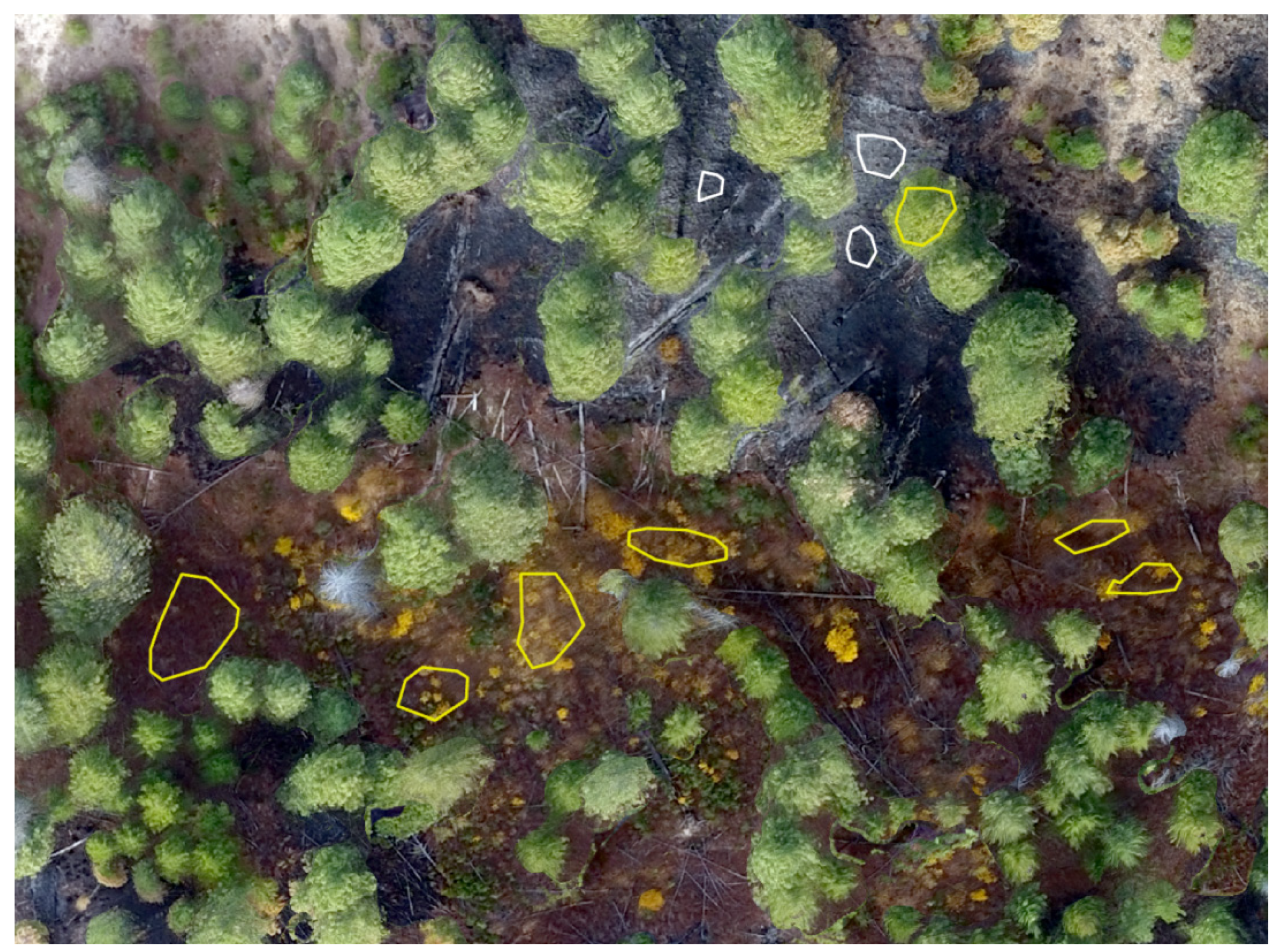
The training data for the SVM was created using the ArcGIS training samples manager using images of burned areas which had obvious differences between burned and unburned regions, as shown in Figure 1. The SVM was trained using the pixel values from the red, green and blue (RGB) bands as well as the user-specified label indicating whether the pixel was burned or not. An average of 200 polygons were digitized into shapefiles using ArcGIS for each fire, with the ratio of burned to un-burned polygons being approximately 50/50. Within the training samples manager, the user labeled each polygon in the shapefile as being either burned or unburned. The ArcGIS Classify tool was used to train an SVM, creating a hyperplane in the RGB space between the pixels labeled as burned and unburned. It then used this trained SVM to classify each of the image pixels based on whether its location in the RGB space put the pixel on the burned or unburned side of the hyperplane [1]. This model was implemented as created by ESRI, along with the hyperparameters established by ESRI [27]. An SVM model was created for each fire using a radial bias function kernel and a soft margin while establishing the hyperplane within the decision space. The SVM hyperparameters including the RBF gamma and soft margin error values are autotuned by ArcGIS using cross validation where a subset of the training pixels are withheld for validation in order to select the optimal hyperparameter values [28]. A new model needed to be trained separately for each fire, and two fires (Cottonwood and Mesa) required splitting the orthomosaic into four tiles each, which created a model for each orthomosaic tile. The orthomosaics were tiled because the ArcGIS SVM implementation cannot process orthomosaics larger than 1 GB. The Gamma values across the models averaged 17.1 and the soft margin error value averaged 11,636. For a more extensive list of SVM hyperparameters, please refer to Appendix B.
MR-CNN: Classifying Tree Crowns
The next step was to locate tree crowns within the orthomosaics. Hamilton [26] found that deep learning using an MR-CNN was highly effective at identifying contiguous pixels representing unburned tree crowns. The MR-CNN is an algorithm for instance segmentation. It detects objects in an image and determines which pixels comprise each object. When classifying an image, the MR-CNN begins by applying a convolutional neural network to extract features from the image. The features extracted from the image are used as input for a region proposal network, which slides over the feature map and detects regions of interest that are likely to contain objects. Each region of interest is evaluated further to determine what type of object is inside the bounding box (in this case, tree or non-tree) and what pixels inside the bounding box comprise the object [29].
Training data for the MR-CNN model consists of images in which the boundaries of all trees are marked with individual polygons. These forested sites primarily contained Pinus Ponderosa (Ponderosa Pine), Populus Trichocarpa (Black Cottonwood), Pseudotsuga Menzieii (Douglas Fir), and Pinus Contorta (Lodgepole Pine). Unmarked areas are assumed to be non-tree. The model is trained using mini-batch gradient descent to minimize a loss function that measures the difference between the model’s output in response to a training image and the training data. The MR-CNN model initiated training with a ResNet-101 backbone that had been pre-trained on the Microsoft COCO dataset [30] which was retrained to detect trees. This tree detection model was set to run on 50 epochs with 100 training steps per epoch. A total of 1024 fully connected layers were used to classify the tree objects, and a minimum probability rate to accept a detected object as a tree was set to 70%. For more information on parameters, please refer to Appendix A. This MR-CNN model was shown to have 90% accuracy which made it effective in automating the process of locating tree crowns [26].
2.2.2. Combining Rasters
Processing an orthomosaic using both the SVM and MR-CNN created two separate rasters, one composed of burned and unburned pixels and the other composed of tree crowns. These two rasters were input into the combine tool in ArcGIS to create one tri-class output raster. Pixels classified as both unburned and surface (non-crown) were reclassified as unburned surface vegetation (surface). Pixels that were classified as both unburned as well as tree crown were reclassified as canopy. Pixels that were classified as burned and surface pixels were reclassified as burned. Pixels classified as burned and canopy pixels were reclassified as canopy. This reclassification is more clearly shown in Table 1.
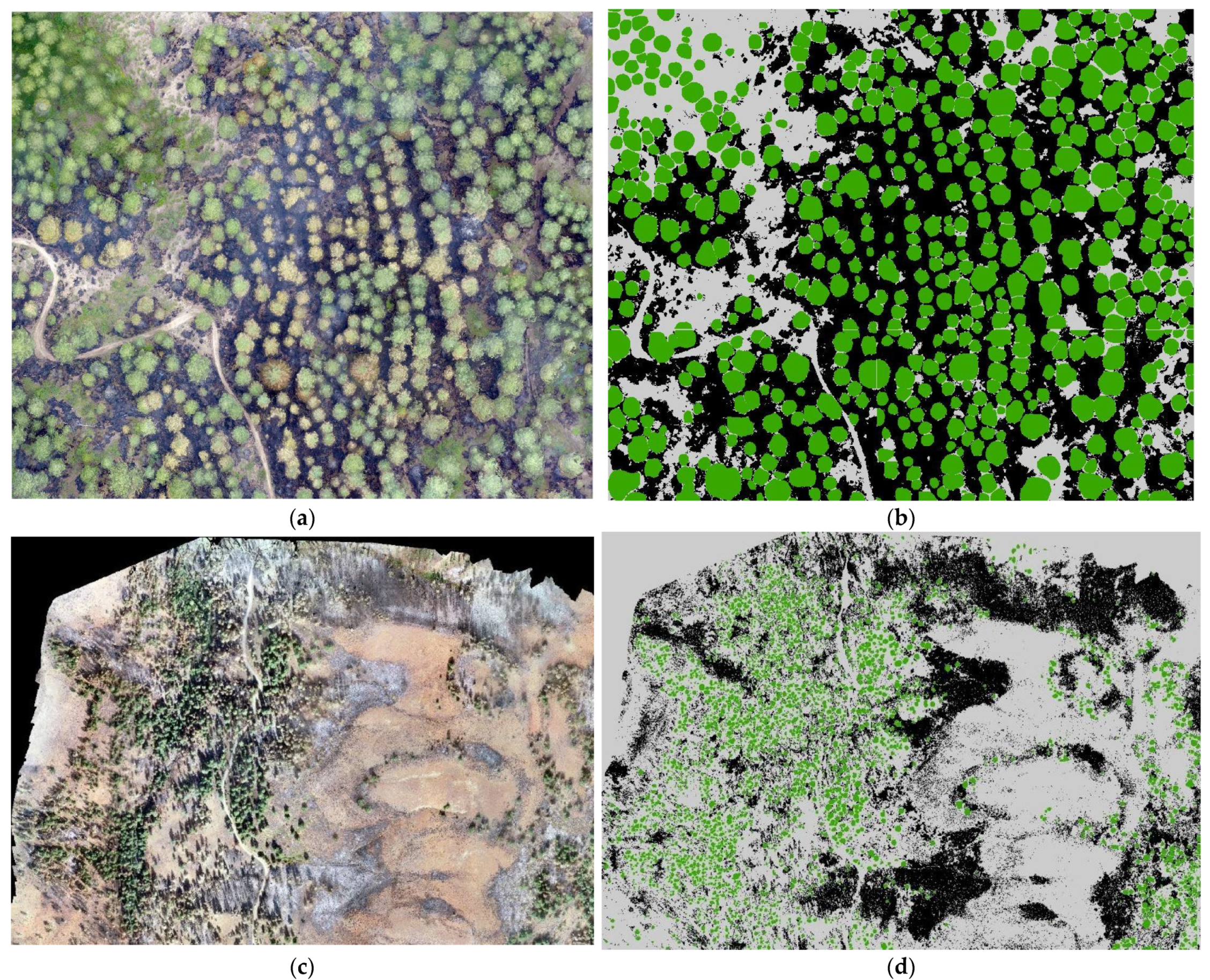
This combined raster results in a single raster comprised of surface, burn and canopy classes as shown in Figure 2.
The choice was made to classify pixels that the object-based MR-CNN classified as tree crown and that the pixel-based SVM classified as burned, as being canopy. This choice was made because the MR-CNN locates canopy pixels based on groups of pixels, while the SVM classifies pixels based solely on individual pixel values. This created a tri-class raster composed of surface, burn, and tree pixels that could be used to locate trees that had experienced sub-crown surface fire.
2.3. Inferring Surface Burn under Unburned Tree Crowns
Sub-crown burn areas will be obscured by unburned canopy cover when observing burn areas within a hyperspatial orthomosaic. When comparing the raster representing unburned, burned and canopy pixels classified from the orthomosaic, if a cluster of pixels comprising a tree crown is completely surrounded by burned pixels, it can be assumed that the fire burned under the tree crown, but did not extend up into the tree crown [1,5].
2.3.1. Sub-Crown Burn Mapping
Once the rasters containing surface, burn and canopy pixels were combined into a single raster, clusters of pixels representing tree crowns that are wholly surrounded by burned pixels are identified with a C++ tool using OpenCV to open the combined tri-class burned, unburned and canopy raster, loading the class values of each pixel into a 2D array. This program which reclassifies burned sub-crown pixel clusters steps through the array systematically from left to right and top to bottom. Whenever the program finds a previously unvisited canopy pixel it iteratively steps through the array, locating every tree pixel in that cluster, and checks if there are only canopy pixels or burn pixels adjacent to each pixel in the tree island. If an entire cluster of tree crown pixels is completely surrounded by burn pixels, then all the pixels in that cluster are reclassified as burn pixels, effectively expanding the burn extent to underneath the tree crown as well. The new raster is created containing the additional sub-crown burned areas reclassified as burned pixels. The raster is then given the same spatial reference as the orthomosaic.
2.3.2. Removing Unburned Tree Noise
Unfortunately, the MR-CNN did not always correctly classify the pixels on the edges of the tree crowns. This caused small clusters of pixels classified by the SVM as unburned to show up between canopy and burned surface pixels, affecting the program’s ability to correctly identify trees that experienced sub-crown burn. To address this unburned tree noise, an additional tool was written to remove clusters of unburned pixels smaller than a specified size by reclassifying the small clusters of unburned pixels as burned. Testing was necessary to find the optimal threshold under which unburned pixel clusters would be reclassified as burned, as discussed in more detail in the following subsection. Increasing the size of the threshold was found to increase the number of true positives (correctly classified as burned) and false positives (incorrectly classified as burned) while decreasing the number of true negatives (correctly classified as unburned) and false negatives (incorrectly classified as unburned vegetation). The assignment of model classification values as well as testing labels to confusion matrix categories are shown in Table 2.
Calibrating the Unburned Pixel Cluster Threshold
Optimizing the unburned pixel cluster threshold under which the clusters of unburned tree noise pixels (pixels between the tree crown and burned pixel clusters (unburned tree noise pixels) were reclassified as burned optimized the specificity, sensitivity, and accuracy, as shown in Equations (1)–(3), respectively.
These methods increase the sensitivity of the SVM by decreasing false negatives due to canopy cover. It is also important that an increase in sensitivity does not result in a significant reduction in specificity. This causes the threshold under which these unburned noise pixels are reclassified as burned to have a significant role in determining which canopy pixels are added to the burn extent and which are not.
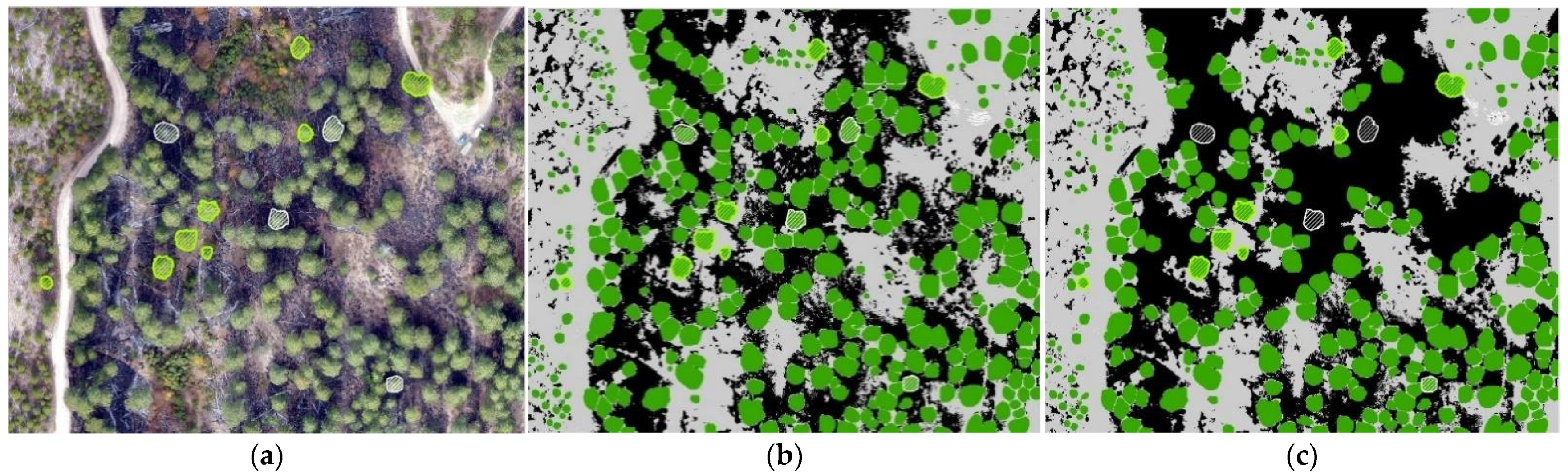
In order to find the optimal threshold value, multiple threshold values were specified for the Unburned Tree Noise Reclassification and then run through Sub-Crown Burn Reclassification. These outputs were then compared to calibration data, which was created using ArcGIS. Polygons were manually digitized around trees in the orthomosaic and marked depending on whether the surface vegetation under the tree crown appeared to have burned or not as shown in Figure 3a. This data was then compared to the Surface Burn Classification output as shown in Figure 3b and the Sub-Crown Burn Reclassification output as shown in Figure 3c. For each threshold, a confusion matrix was created using the ArcGIS Tabulate Area tool. This data was then used to choose which threshold resulted in the highest sensitivity and specificity.
2.4. Creating Validation Data
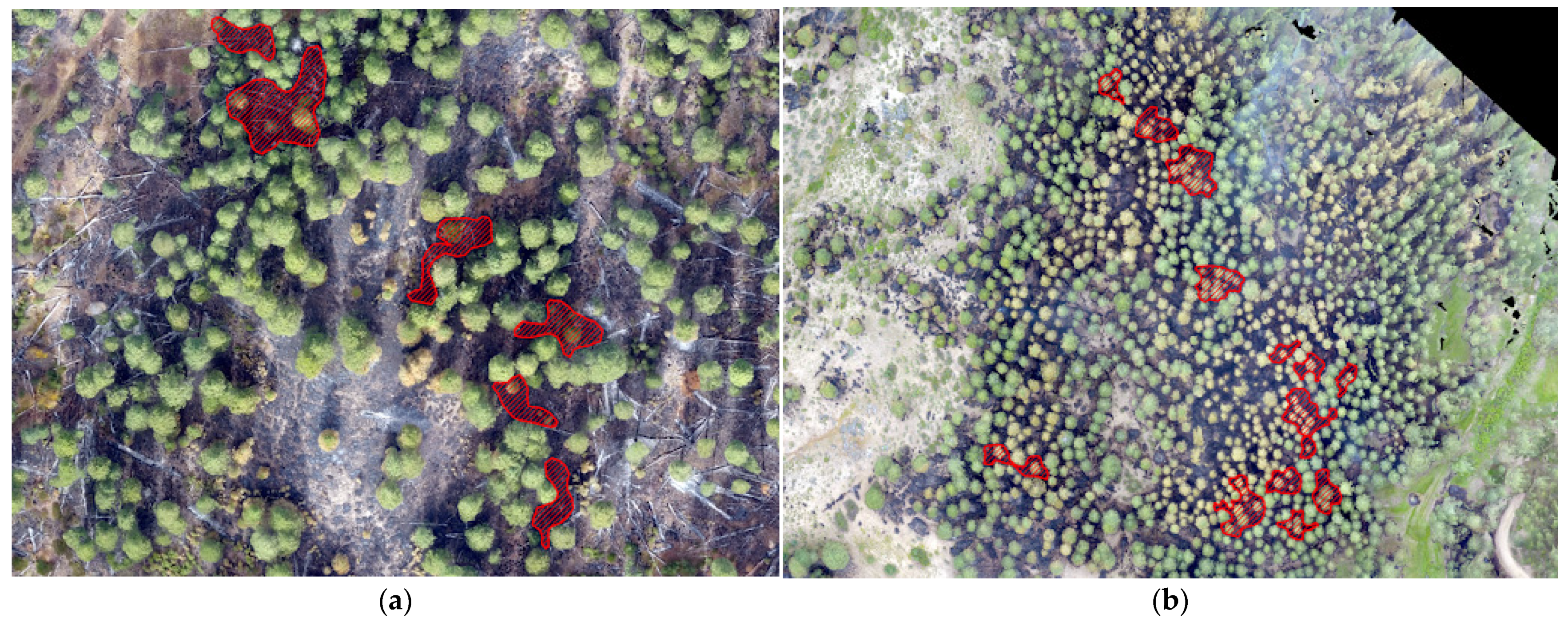
While calibration data was necessary to find the optimal threshold for unburned pixel clusters, validation data was also necessary to validate the updated burn extent mapping after including the sub-crown burn. This was accomplished by manually digitizing polygons using ArcGIS around entire areas of pixels and then classifying them as burned or unburned as shown in Figure 4. The unburned group of pixels encompassed areas of unburned surface vegetation and canopy cover with unburned surface underneath. The burned group of pixels encompassed areas of burned surface vegetation and canopy cover with burned surface underneath.
Validation data was created in ArcGIS for each fire (Hoodoo, Cottonwood, Corner and Mesa) and then compared to the new burn extent which was updated to include the sub-canopy burned areas. Confusion matrices were then created using the ArcGIS Tabulate Area tool. Comparing the validation polygons to the outputs from the Sub-Crown Burn Mapping tools, calculating accuracy, sensitivity, and specificity metrics.
3. Results
This section addresses the results found when classifying burned versus unburned surface vegetation, calibrating the unburned pixel cluster threshold for reclassifying unburned tree noise, and validation of the reclassification of sub-crown burn.
3.1. Accuracy of Methods
There were four post-fire orthomosaics mentioned in the previous section which were used for the project. These orthomosaics were first run through the pixel-based surface burn classification which created a map of the burn extent. Enhanced burn extent maps were then created using the Sub-Crown Burn and Unburned Tree Noise Reclassifications. Both maps from each orthomosaic were compared to validation data that was created for each orthomosaic to determine their accuracies.
3.1.1. Surface Burn Classification Results
Surface burn classification using the SVM with no additional tools or programs had an accuracy of 77% with a specificity of 95% and a sensitivity of 59% over the four orthomosaics as shown in Table 3. The burn classifier had high specificity, meaning that it did well at labeling pixels that were unburned. However, Surface Burn Classification had a low sensitivity meaning that it did poorly at locating pixels that were burned. Sub-Crown Burn Reclassification only increases the number of positives identified by eliminating small groups of surface pixels and adding trees that were surrounded by burn to the burn extent. This increase in positives should contribute to eliminating false negatives, thus increasing the sensitivity of the output.
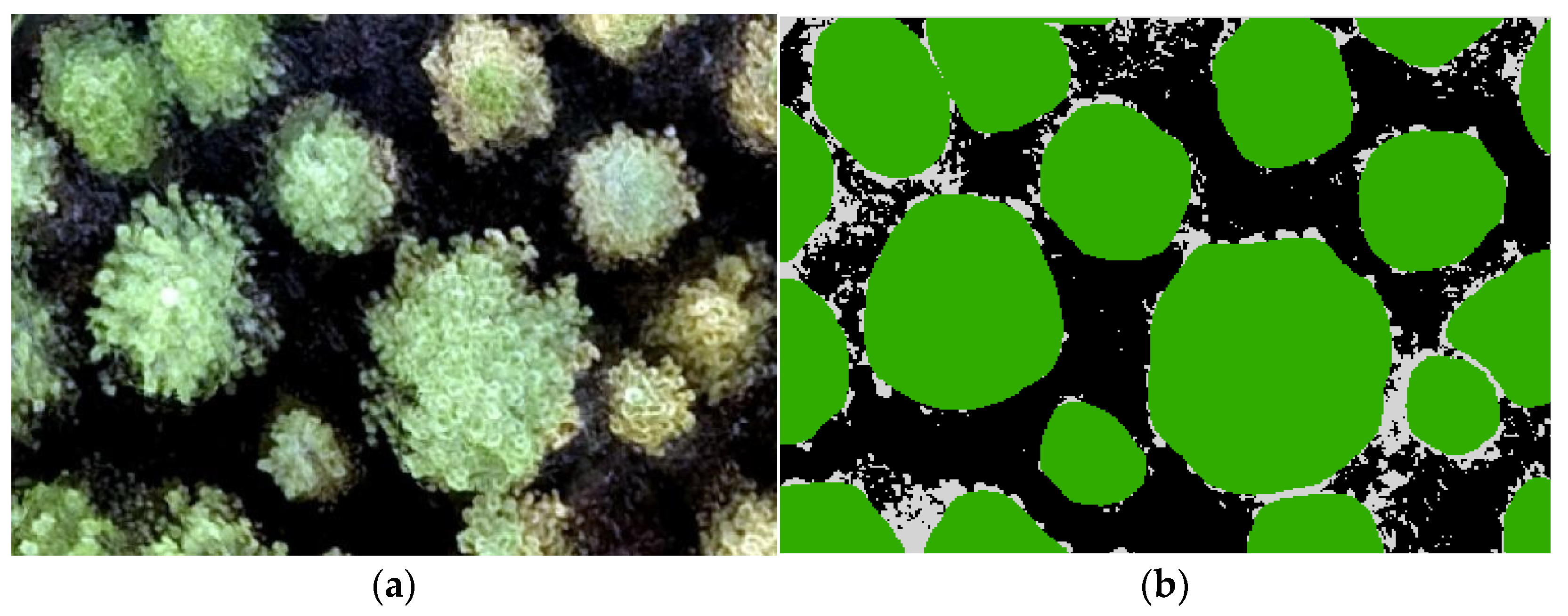
3.1.2. Sub-Crown Burn Reclassification Results
The accuracy from each fire barely increased after Sub-Crown Burn Reclassification, as shown in Table 4. Initially, there was little change between Surface Burn Classification using the SVM and Sub-Crown Burn Reclassification due to how the MR-CNN and SVM were trained. There are some small groups of pixels around the edge of the tree not identified as tree because the MR-CNN does not follow the exact shape of the tree. These pixels are clearly unburned. As a result, the SVM identifies these pixels as such, producing unburned surface pixels when the SVM and MR-CNN classifications are combined instead of correctly identifying these pixels as either canopy or burned. These noise pixels (as seen in Figure 5) cause the clusters of canopy pixels not to be completely surrounded by burn pixels so the burn extent remains the same after running through the Sub-Crown Burn Reclassification. Small groups of noise pixels like this need to be removed in order to improve the accuracy of the Sub-Crown Burn Reclassification.
3.2. Calibrating the Unburned Tree Noise Classifier
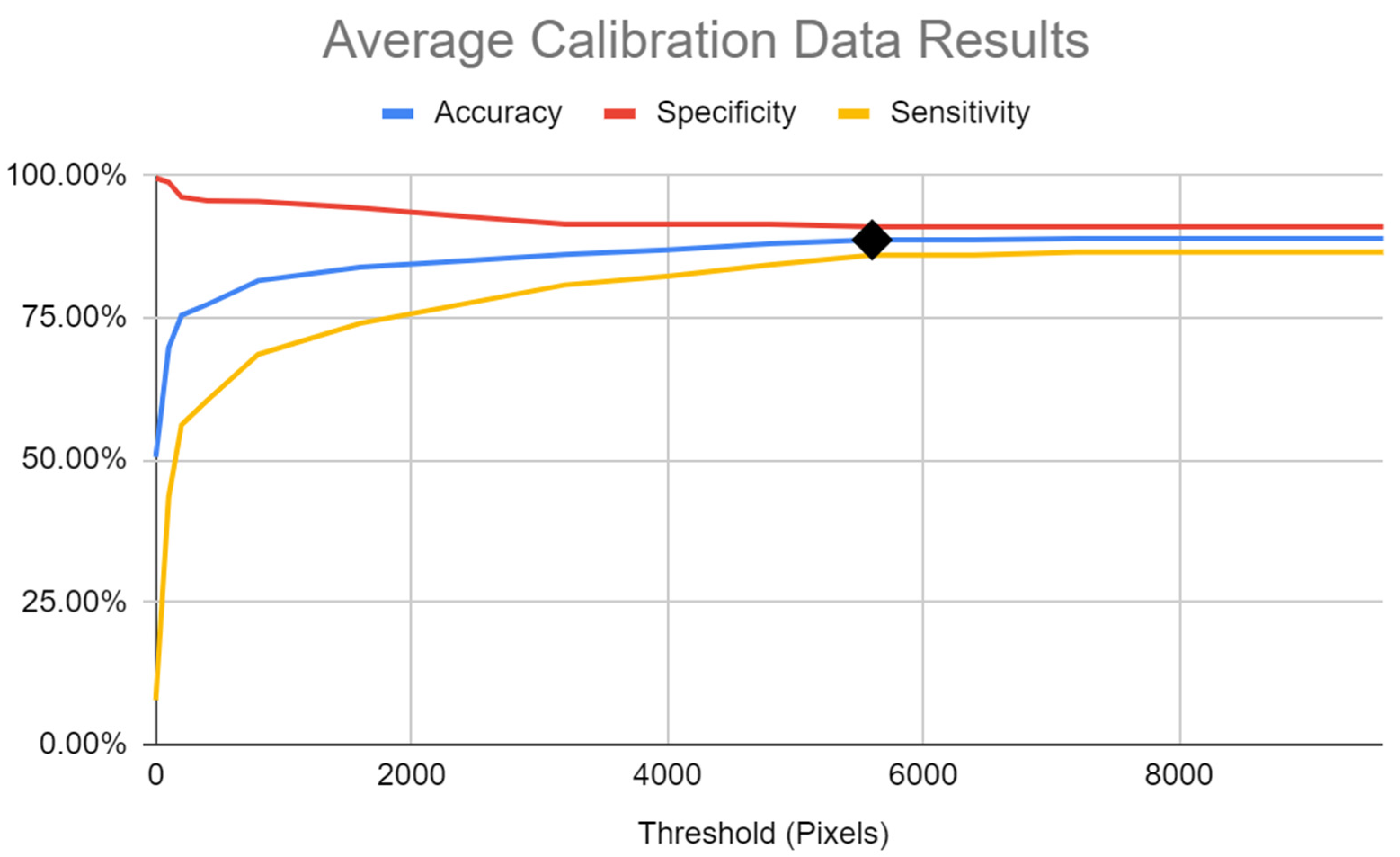
After comparing Sub-Crown Burn Reclassification with 15 different threshold values on the Cottonwood and Hoodoo fires, an unburned pixel cluster threshold of 5600 pixels when removing noise pixels mentioned in the previous section yielded the best results. As the threshold increased, the sensitivity and accuracy followed while the specificity slowly decreased (Table 5 and Figure 6).
The calibration data for determining the optimal noise pixel threshold which the burn extent map was compared to consisted of polygons drawn around individual trees that were labeled by a human observer as being burned underneath and trees that were not labeled as being burned underneath. Table 5 represents the percentage of trees that were correctly identified as part of the burn extent. Thresholds of 4000, 4800 and 5600 pixels all yielded comparable values for accuracy, specificity and sensitivity. 5600 was chosen because it has higher accuracy and sensitivity than all the lower thresholds, with an insignificantly lower specificity than 4000 or 4800. It also has a higher specificity than the higher thresholds, with no significant difference in accuracy or sensitivity. The accuracy, specificity, and sensitivity are nearly the same for 5600, 6400, 7200 and above, but 5600 was chosen because it modifies the fewest number of pixels, and thus the smallest area of the burn extent. This threshold correctly identified 88% of canopy pixels—86% correctly being changed to burn pixels and 91% correctly staying the same (Table 5). This means that an 8-percentage-point decrease in specificity is exchanged for a 78-percentage-point increase in sensitivity and a 38-percentage-point increase in accuracy when a threshold of 5600 is used to reclassify unburned surface noise pixels.
3.3. The Final Burn Extent Output
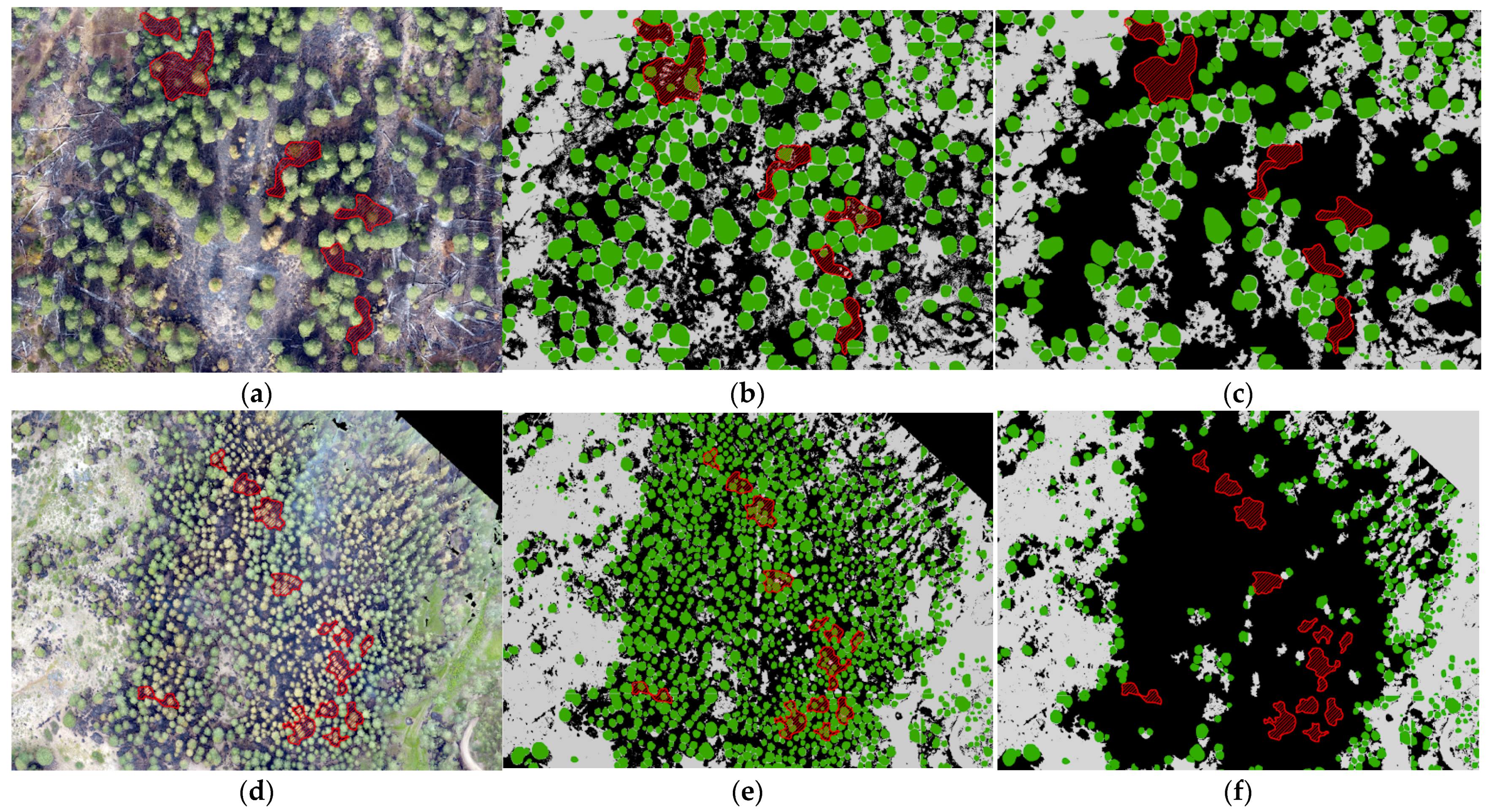
Two burn extent maps with 5cm resolution were created for each fire, one created through Surface Burn Classification using an SVM and the other enhancing the burn extent with the Sub-Crown Burn Reclassification. The Sub-Crown Burn Reclassification uses the surface burn classification raster to eliminate false negatives and increase the sensitivity and accuracy of the burn extent. Since an unburned pixel cluster threshold of 5600 pixels yielded optimal results with calibration data, this number was used to create the final output for the project. Figure 7 shows the input orthomosaics (a&d), mid-process rasters (b&e), and the final output rasters for the Cottonwood and Hoodoo fires (c&f), with validation polygons overlaid.
Since calibration data only focused on individual trees, the increase in accuracy does not cover the entire burn extent. For this reason, validation data was created over larger areas to determine how accurate these methods are at calculating the burn extent.
Validation data, which is a set of polygons that mapped specific areas within and outside the burn extent seen in an orthomosaic, was compared to the reclassified Unburned Tree Noise and Sub-Crown Burn outputs for all four orthomosaics. Based on the results from calibration data, the threshold for reclassification was set to 5600 and resulted in an average accuracy of 86% as shown in Table 6 The outputs maintained a high specificity, meaning that all pixels labeled as part of the burn extent have a 94% chance of being part of the actual burn extent as labeled by a human observer. The Sub-Crown Burn and Unburned Tree Noise Reclassifications drastically improved the sensitivity, resulting in an increase from 59 to 77 percent average sensitivity.
The change in accuracy, specificity, and sensitivity between the Surface Burn Classification using only the SVM, and the burn extent output created by both Sub-Crown Burn and Unburned Tree Noise Reclassification for each of the four different fires is shown in Table 7. Hoodoo and Cottonwood yielded the highest improvements with an increase in accuracy of 17 and 8 percentage points, respectively, as well as an increase in specificity of 32 and 17 percentage points. Table 8 shows the specific differences between Surface Burn Classification and Unburned Tree Noise + Sub-Crown Burn Reclassifications for each fire.
When using a threshold of 5600 pixels to reclassify the Unburned Tree Noise and Sub-Crown Burn, there was an average 18-percentage-point increase in sensitivity with slightly less than a 1-percentage-point drop in specificity, causing the overall accuracy to increase by over 9 percentage points on average. These numbers show that together the Unburned Tree Noise and Sub-Crown Burn Reclassifications create a substantial increase in accuracy and sensitivity while only sacrificing a small amount in specificity.
3.4. Establishment of Statistical Significance
Student’s t-tests were used to determine the statistical significance of the sensitivity results [31]. Sensitivity was chosen as the primary metric for analysis because the main purpose of the Unburned Tree Noise and Sub-Crown Burn Reclassifications was to lower the number of false negatives. Sensitivity is a measure of the percentage of positive burn pixels that were correctly identified, so it is directly related to the false negative percentage. As a result, it was decided to prioritize establishing statistical significance in sensitivity, rather than accuracy.
In this case, a two-tailed paired Student’s t-test was used to directly compare the sensitivity data between the Surface Burn Classification and the Unburned Tree Noise and Sub-Crown Burn Reclassifications [32]. The null hypothesis (H0) was that the Unburned Tree Noise and Sub-Crown Burn Reclassifications created no significant difference in sensitivity compared to the original Surface Burn Classification produced by the support vector machine. Conversely, the alternate hypothesis (H1) was that there is a significant difference in the sensitivity data as a result of the reclassifications. The significance level was set at 0.05, meaning that in order to accept H1 and establish statistical significance, the t-test would have to show at least a 95% certainty that the two data sets are statistically different.
Using the two-tailed paired t-test, a p-value of 0.036 was computed, which is under the significance level of 0.05. This means that H0 is rejected in favor of H1, which claims that there is a significant difference in the sensitivity results between the Surface Burn Classification and the Unburned Tree Noise and Sub-Crown Burn Reclassifications.
To establish statistical significance in the increase in sensitivity after the reclassifications took place, a one-tailed paired t-test was then used. In this case, H0 was that there was a decrease in the sensitivity results after the Unburned Tree Noise and Sub-Crown Burn Reclassifications, while H1 claimed that there was an increase in the sensitivity results after the reclassifications. After running the test, the resulting p-value was 0.018, which is again under the significance level of 0.05. As a result, H0 can be rejected. Therefore statistical analysis demonstrated accepted that the Unburned Tree Noise and Sub-Crown Burn Reclassifications produced a statistically significant increase in sensitivity over relying solely on the Surface Burn Classification for burn extent mapping in favor of the alternate hypothesis that the Surface Burn Classification and the Unburned Tree Noise and Sub-Crown Burn Reclassifications result in an increase in specificity over only using the Surface Burn Classification.
4. Discussion
Land managers often use post-fire mapping data when creating plans to address and mitigate the effects of fire. The post-fire data is relevant for those plans when land managers have prompt access to the data. Using sUASs to produce post-fire data is advantageous because they can be flown over a burned area before plot-based assessments can be safely conducted, allowing for inclusion of the data in the burned area post-fire recovery management plan.
The methodology outlined in this paper enabled the successful identification of tree crowns in the orthomosaic that were totally surrounded by burned surface vegetation. Reclassification of pixels obscured by these tree crowns increased burn extent mapping accuracy by 9 percentage points. More importantly, the sensitivity (classification of burned areas) was improved by 18 percentage points through the inference that the area under the tree which experienced surface fire was mis-classified as unburned due to the unburned tree crown obstructing the burned surface vegetation below.
4.1. Effects of Shadows on Classification and Validation
Typically, aerial photography is done on clear-sky days with bright sunlight to provide good illumination and proper coloration in the photographs. Flights only occurred when there was 10 percent cloud cover or less [33,34]. At solar noon around the summer solstice, lighting and cloud cover produces few to no shadows visible from the air because the shadows are directly under the objects being observed, in this case, the trees. However, if the hyperspatial imagery is acquired early or late in the day or year, when the sun is closer to the horizon, then bright sunlight produces good lighting on one side of the tree but dark shadows on the other side. Shadows are problematic because a burn classifier could mistake shadow pixels for burned pixels, increasing the number of false positives and decreasing specificity. This problem was particularly evident on the Mesa fire where the image acquisition flights were conducted early in the morning during September. To lessen this issue, the SVM used in Surface Burn Classification needed to be retrained, as will be discussed in Section 4.2.
On the other hand, the Hoodoo fire was flown on an overcast day. There were no visible shadows on the orthomosaic and the trees were well lit and clear in the images (as can be seen previously in Figure 2). Flying on an overcast day produces few shadows [35]. Consequently, the flight would not need to be conducted as close to solar noon. This allows for a more flexible time frame in which to conduct image acquisition flights, as well as allowing for longer flight days, providing the weather remains optimal.
4.2. How Training Data Affects the Support Vector Machine
A machine learning algorithm is only as good as the training data that it is given, and any small anomalies (such as shadows) or differences (such as tone of canopy or burned area) will alter the output. Initially, the SVM was trained using burn pixel data from a prescribed burn flown immediately post-fire. Once the model was trained, it was used to classify each of the orthomosaics and resulted in a burn classification output for each of the fires. Because of how and when the orthomosaic was developed, this model led to various levels of success in correctly identifying burn pixels for each fire. One problem that arose when correctly identifying burn pixels was the variation in burn pixel color from fire to fire. The burn extent was various tones of black and brown when hyperspatial imagery was acquired immediately post-fire, whereas burn extent was actually gray when hyperspatial imagery was acquired months after the fire, as observed with the Mesa fire, which was flown 6 weeks post-containment. Also, shadows obstructed the view of the surface depending on the time of day the hyperspatial imagery was acquired. This made it very difficult for the SVM to classify pixels as truly burned rather than a shadow, especially when burned pixels were gray or brown on the orthomosaic. As a result, SVM models were trained separately for each fire using the ArcGIS SVM classification tool.
4.3. Influence of Canopy Cover on Classifications
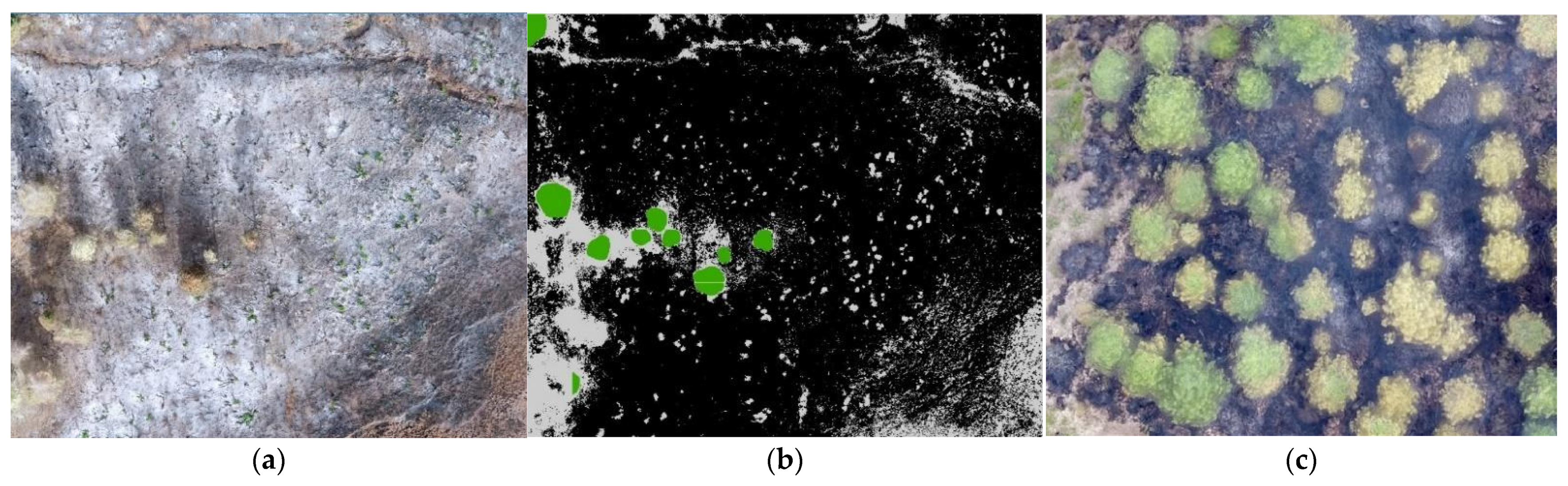
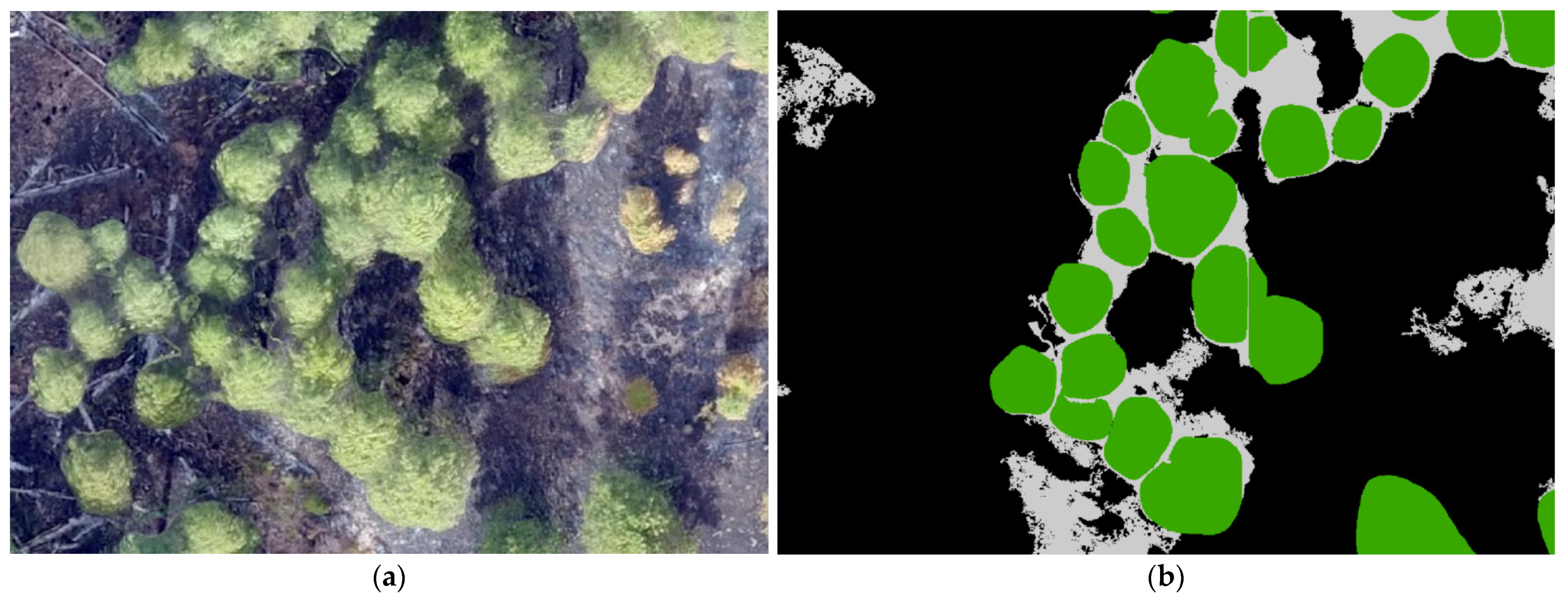
Another factor that affects how well Surface Burn Classification correctly identifies burned pixels is the number of surface pixels visible in the orthomosaic. If the canopy cover on the orthomosaic is too dense, then Surface Burn Classification will be significantly less effective. On the other hand, if there is very little canopy cover, then Surface Burn Classification will correctly identify most of the burn extent (as shown in Figure 8b), but Sub-Crown Burn Reclassification will not be needed, as few tree crowns would be in the burn extent. Burn extent reclassification gave the greatest improvements when there was moderately dense canopy cover as seen in Figure 9c, where Surface Burn Classification can correctly identify the surface and Sub-Crown Burn Reclassification can correctly identify tree crowns surrounded by burn and reclassify them as burned.
4.4. Improving the Results of the Unburned Tree Noise Classifier
5600 pixels was used as the final unburned pixel cluster threshold. Using this threshold and the 5cm spatial resolution of the orthomosaics, the largest cluster of pixels that would be removed is 14 square meters. Other lower thresholds such as 1600 pixels, which could remove a maximum area of 4 square meters and would decrease accuracy by five percentage points, (Table 3) could be used to create similar results with unburn tree noise classification being less likely to remove a small area of truly unburned pixels.
While these tools and methodology greatly improve the accuracy by which sub-canopy surface fires are mapped, there is still room for improvement. An issue that was noticed with some fires was when many unburned tree noise pixels are connected to one another in areas of closed canopy cover as shown in Figure 10a. In this case, the clusters of unburned noise pixels that were incorrectly classified as unburned surface vegetation were not detected because the unburned tree noise pixels were contiguous within a dense stand of trees as shown in Figure 10b, resulting in the collective cluster of unburned tree noise pixels being larger than the unburned tree noise pixel cluster threshold.
To account for this misclassification, machine learning could be used in the future to identify these noise pixels based less on the number of pixels inside the group, and more on the shape and location of the pixel cluster relative to trees and burned patches. Another way to improve the results of the Unburned Tree Noise Classifier is through retraining the MR-CNN. When annotating the training images for the MR-CNN, there was an emphasis on detecting only tree pixels, and for this reason the training data did not go to the very edge of every tree. This caused the output of the MR-CNN not to detect the very edge of the trees, contributing to noise pixels. If this problem were to be addressed, then the unburned tree noise pixel cluster threshold will not need to be set as high, resulting in the removed pixels being more likely to really be noise pixels rather than a small patch of unburned pixels. Doing either of these would produce a more accurate burn extent, with more trees being reclassified as having experienced sub-crown burn.
4.5. Using and Deploying the Methodology
If these methods were to be followed by this team on an additional fire in a time critical environment where managers requested these burn extent products, our previous experience would support being able to have these products available for fire managers within two days of flying the burned area. On the first day, we would be able to get to the fire location, conduct the image acquisition flights, return to our lab, download the images from the drone to a workstation and start Pix4D to generate orthomosaics, then let Pix4d run overnight. On the next day, Pix4D should have completed generating the orthomosaic overnight. The rest of the tools included in this workflow would be able to complete running, generating this burn extent map within a few hours. Additionally, we would be able to also generate the other associated burn extent and severity maps developed with methods previously published by the authors, generating burn severity outputs mapping biomass consumption [1] as well as tree mortality [26] by the end of the day after the imagery was acquired. The ability to quickly produce for fire managers a suite of burn extent and severity maps using these methodologies would be very beneficial for enabling managers to quickly obtain post-fire mapping data in order to more effectively establish and implement post-fire recovery plans.
Currently, this methodology has only been implemented by members of this research effort in the Computer Science Department at Northwest Nazarene University. The workflow necessary to generate the enhanced burn extent is also not user friendly and requires more human interaction than is desirable. This could change in the future with the development of a web-enabled application to run the SVM, MR-CNN, Sub-Crown Burn Classifications, and other tools, to generate enhanced burn extent and other similar results with minimal human interaction.
Additional improvements in runtime performance for the tools used in this methodology could be obtained through additional parallelization of the associated tools. The MR-CNN cannot run on an entire orthomosaic at one time. It breaks the orthomosaic into many smaller tiles, classifies trees within those smaller tiles, then stitches the tiles together again. This has potential for massive parallel processing using a cluster with access to powerful GPUs, cutting runtime even further. A similar process could be applied to the SVM or Sub-Crown Burn Classifications.
While it is much more accurate to map burn extent using hyperspatial sUAS imagery, the mapping extent is limited by current regulatory and technical constraints restricting how large of an area can be flown with an sUAS in a day [26]. During the summers of 2018 and 2019, this research effort utilized sUAS to acquire imagery over 6000 hectares in collaboration with the USDA forest service on the Boise and Payette National Forests [36,37] in southern Idaho. By refining the flight operation procedures, the team was able increase the efficiency and extent of the flights, enabling the acquisition of over 500 hectares in a single day [26]. While acquisition of imagery for very large fires over 1000 hectares may not currently be feasible with these current constraints, there are satellite products currently available which approach a spatial resolution of 50 cm. These very high spatial resolution satellite products may have adequate resolution to be used with this approach, eliminating the image acquisition flight constraints imposed by the use of sUAS.
5. Conclusions
Hamilton [1] showed that live forest canopy foliage obscured sub-crown burned areas, reducing the area within a fire perimeter that machine learning algorithms classified as burned. This methodology improved burn extent mapping in forested ecosystems by enabling the classification of sub-crown burn as being burned despite being obscured by tree crowns. As a result of these methods, sensitivity was increased by 18 percentage points and the accuracy of the burn extent was increased by 9 percentage points over using only a pixel-based SVM, as used previously. This methodology was not found to improve the specificity, which is understandable as these methods were not intended to improve the classification of areas that did not burn.
The resulting improved fire-effects mapping using a combination of pixel-based SVM classification of burned vegetation and an object-based classification of tree crowns with an MR-CNN provides a more usable view of the effects of a wildland fire in forested areas than what was previously used by Hamilton [26]. These more accurate burn extent maps can provide managers with more detailed information about the area where a fire burned than the burn extent maps that are currently available to fire managers.
Author Contributions
Conceptualization, D.H.; methodology, D.H., K.B.; software, K.B.; validation, C.M., B.G.; formal analysis, T.S., C.M. and B.G.; investigation, D.H., K.B.; resources, D.H.; data curation, D.H.; writing—original draft preparation, D.H., K.B., C.M. and B.G.; writing—review and editing, D.H., C.M. and B.G.; visualization, C.M., B.G.; supervision, D.H.; project administration, D.H.; funding acquisition, D.H. All authors have read and agreed to the published version of the manuscript.
Funding
This research was funded by the USDA Forest Service Boise National Forest, Forest Service Agreement No, 18-CS-11040200-0025.
Institutional Review Board Statement
Not applicable.
Informed Consent Statement
Not applicable.
Data Availability Statement
All data and source code from this project is available at https://firemap.nnu.edu/forest-burn-extent.
Acknowledgments
We would like to acknowledge the students in the Northwest Nazarene University Department of Math and Computer Science who have helped with different aspects of this effort, including current and former students Jacob Winters, Nicholas Hamilton, Cody Robbins, Enoch Levandovsky, Gabriel Johnson, Austin White, Aleesha Chavez, and Andrew Welk. Additionally, we would like to acknowledge Northwest Nazarene University who funded the research efforts of many of the students mentioned as well as Dr Kathy Becker who edited this manuscript.
Conflicts of Interest
The authors declare no conflict of interest.
Appendix A
Full List of Parameters for MR-CNN Tree Object Detection Model.

| Parameter Type | Parameter Value |
|---|---|
| GPU Count | 1 |
| Number of images to train per GPU | 1 1 |
| Number of training steps per epoch | 100 1 |
| Number of epochs | 50 1 |
| Number of validation steps at the end of every training epoch | 50 |
| Backbone network structure | resnet101 |
| FPN Pyramid backbone strides | [4,8,16,32,64] |
| Size of fully connected layers in the classification graph | 1024 |
| Size of the top-down layers used to build the feature pyramid | 256 |
| Number of classification classes | 2, Tree & Background 1 |
| Length of square anchor side in pixels | (32,64,128,256,512) |
| Width to Height ratios of anchors at each cell | [0.5,1,2] |
| Anchor stride | Created for every cell |
| Non-max suppression threshold to filter RPN proposals | 0.7 |
| How many anchors per image to use for RPN training | 256 |
| ROIs kept after tf.nn.top_k and before non-maximum suppression | 6000 |
| ROIs kept after non-maximum suppression—training | 2000 |
| ROIs kept after non-maximum suppression—inference | 1000 |
| Mask reduced resolution to reduce memory load (height, width) | (56,56) |
| Input image resize shape | Crop 1 |
| Input image resize minimum dimension | 1024 1 |
| Input image resize maximum dimension | 1024 |
| Color channels per image | RGB |
| Image mean pixel (RGB) | [123.7, 116.8, 103.9] |
| Number of ROIs per image to feed to classifier/mask heads | 200 |
| Percent of positive ROIs used to train classifier/mask heads | 0.33 |
| ROI Pool Size | 7 |
| ROI Mask Pool Size | 14 |
| Shape of output mask | [28,28] |
| Maximum number of ground truth instances to use in one image | 100 |
| Bounding box refinement standard deviation for RPN and final detections RPN_BBOX_STD_DEV BBOX_STD_DEV | np.array([0.1, 0.1, 0.2, 0.2]) |
| Max number of final detections | 100 |
| Minimum probability value to accept a detected instance | 0.7 |
| Non-maximum suppression threshold for detection | 0.3 |
| Learning Rate | 0.001 |
| Learning Momentum | 0.9 |
| Weight decay regularization | 0.0001 |
| Loss weights for more precise optimization and can be used for R-CNN training setup. | LOSS_WEIGHTS = {“ rpn_class_loss”: 1., “rpn_bbox_loss”: 1., “mrcnn_class_loss”: 1., “mrcnn_bbox_loss”: 1., “mrcnn_mask_loss”: 1. } |
| Use RPN ROIs or externally generated ROIs for training | Use RPN ROIs |
| Train or freeze batch normalization layers | Freeze |
| Gradient norm clipping | 5.0 |
1 Except for these values, all other parameters were set to their default value. These parameters were specifically adjusted to handle the classification of tree objects.
Appendix B
Full list of hyperparameters for ArcGIS support vector machine surface burn detection models which were found in the SVM output classifier definition (.ecd) file that is generated by ArcGIS Pro when the SVM trains and classifies an image.
| Number of Classes | 2—Burn, Unburn |
| Maximum Number of Samples | 500 |
| SVM Type | c_cvc |
| Kernel Type | Rbf |
| Average Cross Validation Rate | 0.9232 +/− 0.0394 |
| Average Gamma | 17.1066 +/− 9.6475 |
| Average costC | 11,636.6961 +/− 7261.51 |
| Average Number of Support Vectors | 1882 +/− 1752.8244 |
NOTE: Since at least one separate Burn Detection Model needed to be trained for each fire, how the average values were calculated are listed below.
Cross Validation Rate, Gamma, CostC and Total Support Vectors hyperparameters varied between each of the images run through the ArcGIS Support Vector Machine. Following are the values for each hyperparameter for each of the images. As mentioned in Section 2.2.1, the Mesa and Cottonwood fires were split into four tiles each to accommodate restrictions on size of imagery that can be classified.
| Fire | Section | Cross Validation Rate | Gamma | CostC | Total Support Vectors |
|---|---|---|---|---|---|
| Mesa | Quad 0 | 0.90200 | 4.00000 | 23,170.47501 | 702 |
| Quad 1 | 0.94733 | 2.00000 | 32,768.00000 | 433 | |
| Quad 2 | 0.97233 | 11.31371 | 5792.61875 | 242 | |
| Quad 3 | 0.94840 | 2.00000 | 16,384.00000 | 348 | |
| Average | 0.94252 | 4.82843 | 19,528.77344 | 1725 | |
| Standard Deviation | 0.02544 | 3.83227 | 9837.56392 | 170.33405 | |
| Cottonwood | Quad 0 | 0.87025 | 32.00000 | 11,585.23750 | 1250 |
| Quad 1 | 0.89700 | 22.62742 | 23,170.47501 | 1053 | |
| Quad 2 | 0.87075 | 32.00000 | 23,170.47501 | 1249 | |
| Quad 3 | 0.87925 | 32.00000 | 11,585.23750 | 1228 | |
| Average | 0.87931 | 29.65685 | 17,377.85625 | 4780 | |
| Standard Deviation | 0.01082 | 4.05845 | 5792.61875 | 82.45302 | |
| Corner | 0.97800 | 22.62742 | 1448.15469 | 277 | |
| Hoodoo | 0.89300 | 11.31371 | 8192.00000 | 746 |
References
- Hamilton, D.; Pacheco, R.; Myers, B.; Peltzer, B. kNN vs. SVM: A Comparison of Algorithms. In Proceedings of the Fire Continuum—Preparing for the Future of Wildland Fire, Missoula, MT, USA, 21–24 May 2018; p. 95. Available online: https://www.fs.usda.gov/treesearch/pubs/60581 (accessed on 22 September 2021).
- Zhang, R.; Ma, J. An improved SVM method P-SVM for classification of remotely sensed data. Int. J. Remote Sens. 2008, 29, 6029–6036. [Google Scholar] [CrossRef]
- Hamilton, D.; Myers, B.; Branham, J.B. Evaluation of Texture as an Input of Spatial Context for Machine Learning Mapping of Wildland Fire Effects. Signal Image Process. Int. J. 2017, 8, 1–11. [Google Scholar] [CrossRef]
- Hamilton, D. Improving Mapping Accuracy of Wildland Fire Effects from Hyperspatial Imagery Using Machine Learning; The University of Idaho: Moscow, ID, USA, 2018. [Google Scholar]
- Scott, J.H.; Reinhardt, E.D.; Station, R.M.R. Assessing Crown Fire Potential by Linking Models of Surface and Crown Fire Behavior; USDA Forest Service Research Paper; U.S. Department of Agriculture, Forest Service, Rocky Mountain Research Station: Fort Collins, CO, USA, 2001. [Google Scholar] [CrossRef] [Green Version]
- Wildland Fire Leadership Council. The National Strategy: The Final Phase in the Development of the National Cohesive Wildland Fire Management Strategy. April 2014. Available online: https://www.forestsandrangelands.gov/documents/strategy/strategy/CSPhaseIIINationalStrategyApr2014.pdf (accessed on 22 September 2021).
- Hoover, K.; Hanson, L.A. “Wildfire Statistics”. Congressional Research Service. October 2019. Available online: https://crsreports.congress.gov/product/pdf/IF/IF10244 (accessed on 14 May 2020).
- National Interagency Fire Center (NIFC). Suppression Costs. 2020. Available online: https://www.nifc.gov/fireInfo/fireInfo_documents/SuppCosts.pdf (accessed on 18 May 2020).
- National Interagency Fire Center (NIFC). Wildland Fire Fatalities by Year. National Interagency Fire Center. 2020. Available online: https://www.nifc.gov/safety/safety_documents/Fatalities-by-Year.pdf (accessed on 18 May 2020).
- Zhou, G.; Li, C.; Cheng, P. Unmanned aerial vehicle (UAV) real-time video registration for forest fire monitoring. In Proceedings of the 2005 IEEE International Geoscience and Remote Sensing Symposium, Seoul, Korea, 29 July 2005. [Google Scholar]
- Insurance Information Institute. Available online: https://www.iii.org/fact-statistic/facts-statistics-wildfires#Wildfires%20By%20State,%202019 (accessed on 18 May 2020).
- Gitas, I.Z.; Mitri, G.H.; Ventura, G. Object-based image classification for burned area mapping of Creus Cape, Spain, using NOAA-AVHRR imagery. Remote Sens. Environ. 2004, 92, 409–413. [Google Scholar] [CrossRef]
- Hamilton, D.; Hann, W. Mapping landscape fire frequency for fire regime condition class. In Proceedings of the Large Fire Conference, Missoula, MT, USA, 19–23 May 2014; p. 111. Available online: https://www.fs.fed.us/rm/pubs/rmrs_p073.pdf (accessed on 22 September 2021).
- Brewer, C.K.; Winne, J.C.; Redmond, R.L.; Opitz, D.W.; Mangrich, M.V. Classifying and Mapping Wildfire Severity. Photogramm. Eng. Remote Sens. 2005, 71, 1311–1320. [Google Scholar] [CrossRef] [Green Version]
- Kontoes, C.; Poilvé, H.; Florsch, G.; Keramitsoglou, I.; Paralikidis, S. A comparative analysis of a fixed thresholding vs. a classification tree approach for operational burn scar detection and mapping. Int. J. Appl. Earth Obs. Geoinf. 2009, 11, 299–316. [Google Scholar] [CrossRef]
- Seydi, S.; Akhoondzadeh, M.; Amani, M.; Mahdavi, S. Wildfire Damage Assessment over Australia Using Sentinel-2 Imagery and MODIS Land Cover Product within the Google Earth Engine Cloud Platform. Remote Sens. 2021, 13, 220. [Google Scholar] [CrossRef]
- Hawbaker, T.J.; Vanderhoof, M.K.; Schmidt, G.L.; Beal, Y.-J.; Picotte, J.J.; Takacs, J.D.; Falgout, J.T.; Dwyer, J.L. The Landsat Burned Area algorithm and products for the conterminous United States. Remote Sens. Environ. 2020, 244, 111801. [Google Scholar] [CrossRef]
- Boschetti, L.; Roy, D.P.; Justice, C.O. International Global Burned Area Satellite Product Validation Protocol Part I—Production and Standardization of Validation Reference Data. 2009. Available online: https://lpvs.gsfc.nasa.gov/PDF/BurnedAreaValidationProtocol.pdf (accessed on 17 August 2021).
- Hamilton, D.; Bowerman, M.; Colwell, J.; Donohoe, G.; Myers, B.; Donohoe, G. Spectroscopic Analysis for Mapping Wildland Fire Effects from Remotely Sensed Imagery. J. Unmanned Veh. Syst. 2017, 5, 146–158. [Google Scholar] [CrossRef] [PubMed] [Green Version]
- Lentile, L.B.; Holden, Z.A.; Smith, A.; Falkowski, M.J.; Hudak, A.T.; Morgan, P.; Lewis, S.A.; Gessler, P.E.; Benson, N.C. Remote sensing techniques to assess active fire characteristics and post-fire effects. Int. J. Wildland Fire 2006, 15, 319–345. [Google Scholar] [CrossRef]
- Lewis, S.A.; Robichaud, P.R.; Frazier, B.E.; Wu, J.Q.; Laes, D.Y. Using hyperspectral imagery to predict post-wildfire soil water repellency. Geomorphology 2008, 95, 192–205. [Google Scholar] [CrossRef]
- Monitoring Trends in Burn Severity. Available online: https://mtbs.gov/ (accessed on 9 November 2017).
- Sparks, A.M.; Boschetti, L.; Smith, A.; Tinkham, W.T.; Lannom, K.O.; Newingham, B.A. An accuracy assessment of the MTBS burned area product for shrub steppe fires in the northern Great Basin, United States. Int. J. Wildland Fire 2014, 24, 70–78. [Google Scholar] [CrossRef]
- Eidenshink, J.; Schwind, B.; Brewer, K.; Zhu, Z.; Quayle, B.; Howard, S. A Project for Monitoring Trends in Burn Severity. Fire Ecol. 2007, 3, 3–21. [Google Scholar] [CrossRef]
- Hamilton, D.; Hamilton, N.; Myers, B. Evaluation of Image Spatial Resolution for Machine Learning Mapping of Wildland Fire Effects. In Proceedings of the SAI Intelligent Systems Conference, London, UK, 5–6 September 2019; pp. 400–415. [Google Scholar]
- Hamilton, D.; Brothers, K.; Jones, S.; Colwell, J.; Winters, J. Wildland Fire Tree Mortality Mapping from Hyperspatial Imagery Using Machine Learning. Remote Sens. 2021, 13, 290. [Google Scholar] [CrossRef]
- Classify—ArcGIS Pro Documentation. Available online: https://pro.arcgis.com/en/pro-app/2.7/help/analysis/image-analyst/classify.htm (accessed on 22 July 2021).
- ESRI Support Services. Train SVM Classifier values for Kernel, Gamma, C-Values; Private Email Correspondence, 27th August 2021; ESRI: West Redlands, CA, USA, 2021. [Google Scholar]
- He, K.; Gkioxari, G.; Dollar, P.; Girshick, R. Mask R-CNN. In Proceedings of the 2017 IEEE International Conference on Computer Vision (ICCV), Venice, Italy, 22–29 October 2017. [Google Scholar]
- Tsung-Yi, L.; Maire, M.; Belonge, S.; Hays, J.; Perona, P.; Ramanan, D.; Dollár, P.; Zitnick, C.L. Microsoft coco: Common objects in context. In European Conference on Computer Vision; Springer: Cham, Switzerland, 2014; pp. 740–755. [Google Scholar]
- Brownlee, J. How to Calculate Parametric Statistical Hypothesis Tests in Python. Machine Learning Mastery. 17 May 2018. Available online: https://machinelearningmastery.com/parametric-statistical-significance-tests-in-python/ (accessed on 3 June 2021).
- Wilkerson, S. Application of the Paired t-test. XULAneXUS 2008, 5, 6. [Google Scholar]
- Tellidis, I.; Levin, E. Photogrammetric Image Acquisition with Small Unmanned Aerial Systems. In Proceedings of the ASPRS 2014 Annual Conference, Louisville, KY, USA, 23–28 March 2014; p. 12. [Google Scholar]
- USDA Farm Service Agency. NAIP Imagery, National-Content. 2021. Available online: https://fsa.usda.gov/programs-and-services/aerial-photography/imagery-programs/naip-imagery/index (accessed on 25 May 2021).
- Robinson, E.M. Crime Scene Photography; Academic Press: Cambridge, MA, USA, 2016. [Google Scholar]
- Goodwin, J.; Hamilton, D. Archaeological Imagery Acquisition and Mapping Analytics Development; Boise National Forest: Boise, ID, USA, 2019. [Google Scholar]
- Calkins, A.; Hamilton, D. Archaeological Imagery Acquisition and Mapping Analytics Development; Boise National Forest: Boise, ID, USA, 2018. [Google Scholar]
Figure 1.
Example of data used to train SVM. Polygons in white were drawn to classify the pixels as burned, and polygons in green were drawn to classify the pixels as unburned.
Figure 1.
Example of data used to train SVM. Polygons in white were drawn to classify the pixels as burned, and polygons in green were drawn to classify the pixels as unburned.

Figure 2.
(a) Orthomosaic imagery from the Hoodoo fire (b) Combined raster results with surface represented by gray, burn represented by black, and canopy represented by green. (c) Orthomosaic imagery from the Mesa fire (d) Combined raster from the Mesa fire.
Figure 2.
(a) Orthomosaic imagery from the Hoodoo fire (b) Combined raster results with surface represented by gray, burn represented by black, and canopy represented by green. (c) Orthomosaic imagery from the Mesa fire (d) Combined raster from the Mesa fire.

Figure 3.
(a) Cottonwood orthomosaic imagery with calibration data polygons overlaid. The bright green polygons are trees that were marked by the human as trees, and the white polygons are trees that are completely surrounded by burned pixels, implying that the surface underneath the crown is burned, and are marked by the human as burned. (b) Combined raster output from the Cottonwood fire with calibration data polygons. (c) Output from the Sub-Crown Burn Mapping tools on Cottonwood. This image shows what the Sub-Crown Burn Mapping tools do and how they compare to calibration data that was created.

Figure 4.
These images contain an orthomosaic with validation data overlaid on top. The polygons in red contain areas of burned surface vegetation and canopy cover that is burned underneath. These areas in red should be considered part of the burn extent, and these polygons were drawn to validate our classifications. (a) Image from the Cottonwood prescribed burn (b) Image from the Hoodoo prescribed burn.

Figure 5.
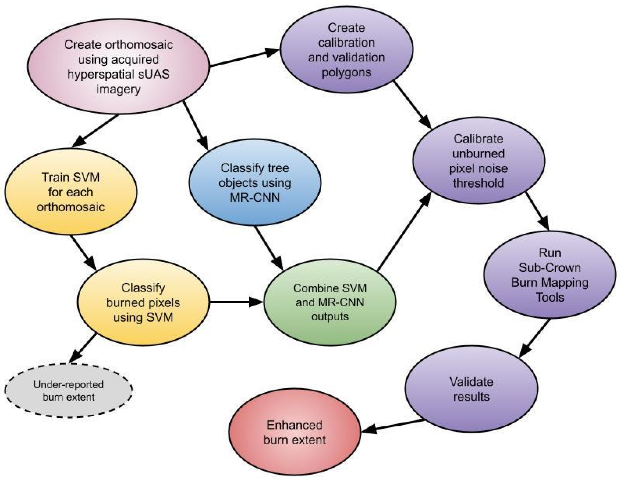
A flowchart summarizing the workflow to create an enhanced burn extent for a burned area. Each bubble is a significant step in the process. The colors have little significance, only showing very general correlations between bubbles. The dashed bubble is not part of the workflow; it shows what step produced the under-reported burn extent used previously.
Figure 5.
A flowchart summarizing the workflow to create an enhanced burn extent for a burned area. Each bubble is a significant step in the process. The colors have little significance, only showing very general correlations between bubbles. The dashed bubble is not part of the workflow; it shows what step produced the under-reported burn extent used previously.

Figure 6.
(a) Orthomosaic imagery from the Hoodoo fire. (b) Combined raster results with unburned surface represented by white, burned represented by black, and unburned canopy represented by green. Most of the surface pixels in (b) are noise caused by difference between the SVM unburned classification and the MR-CNN tree crown classification.

Figure 7.
This graph is a visual representation of the information presented in Table 5, excluding the row for SVM results.
Figure 7.
This graph is a visual representation of the information presented in Table 5, excluding the row for SVM results.

Figure 8.
(a) An example from the Mesa fire that shows low canopy cover. (b) This figure shows a mostly identified burn extent without the need for Sub-Crown Burn Reclassification using the imagery from (a). (c) An example from the Hoodoo fire that shows high amounts of canopy cover with low density.

Figure 9.
(a) Cottonwood fire orthomosaic with validation data overlaid on top. The polygons in red encompass part of the burn extent. (b) Cottonwood fire combined raster outputs displaying the canopy pixels and burn pixels. (c) Final Cottonwood fire raster outputs after having reclassified sub-crown burn and unburned tree noise. (d) Hoodoo fire orthomosaic with validation data. (e) Hoodoo fire combined raster outputs and validation data (f) Hoodoo fire Sub-Crown Burn Reclassification output with validation data polygons.

Figure 10.
(a) Part of the Cottonwood fire where the trees are clearly burned underneath. (b) The same part of the Cottonwood fire with the Sub-Canopy Burn Mapping Tools output overlaid. It can be seen that a large section of trees in the middle of the image are not removed due to a large group of noise surface pixels surrounding them.

Table 1.
Reclassification.
| Input | Output |
|---|---|
| Unburn & Surface | Surface |
| Burn & Surface | Burn |
| Unburn & Canopy | Canopy |
| Burn & Canopy | Canopy |
Table 2.
Assignment of Classification Values to Confusion Matrix Categories.
| Human Classification | Computer Classification | Result |
|---|---|---|
| Unburned | Surface | True Negative |
| Unburned | Canopy | True Negative |
| Unburned | Burned | False Positive |
| Burned | Surface | False Negative |
| Burned | Canopy | False Negative |
| Burned | Burned | True Positive |
Table 3.
Support Vector Machine Surface Burn Classification Results.
| Classifier | Accuracy | Specificity | Sensitivity |
|---|---|---|---|
| Surface Burn Classification | 77.6% | 95.3% | 59.4% |
Table 4.
Surface Burn Classification and Sub-Crown Burn Reclassification Results.
| Classifier | Accuracy | Specificity | Sensitivity |
|---|---|---|---|
| Surface Burn Classification | 77.6% | 95.3% | 59.4% |
| Sub-Crown Burn Reclassification | 77.6% | 95.3% | 59.3% |
Table 5.
Calibration data, with the optimal unburned pixel cluster threshold that was selected highlighted in green and the results from the SVM surface burn classification in orange.
Table 5.
Calibration data, with the optimal unburned pixel cluster threshold that was selected highlighted in green and the results from the SVM surface burn classification in orange.
| Calibration Data Averages | |||
|---|---|---|---|
| Threshold | Accuracy | Specificity | Sensitivity |
| SVM | 50.6% | 99.5% | 7.5% |
| 0 | 50.6% | 99.5% | 7.9% |
| 100 | 69.7% | 98.8% | 43.6% |
| 200 | 75.4% | 96.2% | 56.2% |
| 400 | 77.3% | 95.5% | 60.4% |
| 800 | 81.5% | 95.4% | 68.6% |
| 1600 | 83.9% | 94.3% | 74.0% |
| 2400 | 85.0% | 92.8% | 77.4% |
| 3200 | 86.1% | 91.4% | 80.8% |
| 4000 | 86.9% | 91.4% | 82.3% |
| 4800 | 88.0% | 91.4% | 84.3% |
| 5600 | 88.6% | 91.0% | 86.0% |
| 6400 | 88.6% | 91.0% | 86.0% |
| 7200 | 88.9% | 91.0% | 86.5% |
| 8000 | 88.9% | 91.0% | 86.5% |
| 8800 | 88.9% | 91.0% | 86.5% |
| 9600 | 88.9% | 91.0% | 86.5% |
Table 6.
Average Validation Data Results across all fires.
| Classifier | Accuracy | Specificity | Sensitivity |
|---|---|---|---|
| Surface Burn Classification | 77.6% | 95.3% | 59.4% |
| Unburned Tree Noise + Sub-Crown Burn Reclassifications | 86.7% | 94.6% | 77.7% |
| Average Difference | +9.1 | −0.6 | +18.3 |
Table 7.
Changes in Accuracy, Specificity, and Sensitivity for Each Fire Surveyed.
| Fire | Classification | Accuracy | Specificity | Sensitivity |
|---|---|---|---|---|
| Hoodoo | Initial Surface Burn Classification | 81.9% | 99.4% | 66.7% |
| Noise & Sub-Crown Reclassifications | 99.4% | 99.3% | 99.5% | |
| Corner | Initial Surface Burn Classification | 65.0% | 96.0% | 29.2% |
| Noise & Sub-Crown Reclassifications | 70.0% | 95.8% | 40.2% | |
| Cottonwood | Initial Surface Burn Classification | 84.6% | 96.2% | 71.3% |
| Noise & Sub-Crown Reclassifications | 92.6% | 95.8% | 88.9% | |
| Mesa | Initial Surface Burn Classification | 79.0% | 89.5% | 70.3% |
| Noise & Sub-Crown Reclassifications | 84.6% | 87.6% | 82.1% | |
| Average | Initial Surface Burn Classification | 77.6% | 95.3% | 59.4% |
| Noise & Sub-Crown Reclassifications | 86.7% | 94.6% | 77.7% |
Table 8.
Improved Accuracy Using Unburned Tree Noise and Sub-Crown Burn Reclassifications.
| Fire | Accuracy | Specificity | Sensitivity |
|---|---|---|---|
| Hoodoo | +17.6 | −0.1 | +32.9 |
| Corner | +5.0 | −0.2 | +11.0 |
| Cottonwood | +8.1 | −0.3 | +17.6 |
| Mesa | +5.6 | −1.9 | +11.8 |
| Average Difference | +9.1 | −0.6 | +18.3 |
Publisher’s Note: MDPI stays neutral with regard to jurisdictional claims in published maps and institutional affiliations. |
© 2021 by the authors. Licensee MDPI, Basel, Switzerland. This article is an open access article distributed under the terms and conditions of the Creative Commons Attribution (CC BY) license (https://creativecommons.org/licenses/by/4.0/).
Share and Cite
MDPI and ACS Style
Hamilton, D.; Brothers, K.; McCall, C.; Gautier, B.; Shea, T. Mapping Forest Burn Extent from Hyperspatial Imagery Using Machine Learning. Remote Sens. 2021, 13, 3843. https://0-doi-org.brum.beds.ac.uk/10.3390/rs13193843
AMA Style
Hamilton D, Brothers K, McCall C, Gautier B, Shea T. Mapping Forest Burn Extent from Hyperspatial Imagery Using Machine Learning. Remote Sensing. 2021; 13(19):3843. https://0-doi-org.brum.beds.ac.uk/10.3390/rs13193843
Chicago/Turabian StyleHamilton, Dale, Kamden Brothers, Cole McCall, Bryn Gautier, and Tyler Shea. 2021. "Mapping Forest Burn Extent from Hyperspatial Imagery Using Machine Learning" Remote Sensing 13, no. 19: 3843. https://0-doi-org.brum.beds.ac.uk/10.3390/rs13193843
Note that from the first issue of 2016, this journal uses article numbers instead of page numbers. See further details here.