
Global Land High-Resolution Cloud Climatology Based on an Improved MOD09 Cloud Mask
by
 , and
, and
Shuyan Zhang
1,2, 
Yong Ma
1,*,
Fu Chen
1,
Erping Shang
1,
Wutao Yao
1,
Yubao Qiu
1 and
Jianbo Liu
1 1
Aerospace Information Research Institute, Chinese Academy of Sciences, Beijing 100094, China
2
School of Electronic, Electrical and Communication Engineering, University of Chinese Academy of Sciences, Beijing 100049, China
*
Author to whom correspondence should be addressed.
Remote Sens. 2021, 13(19), 3997; https://0-doi-org.brum.beds.ac.uk/10.3390/rs13193997
Submission received: 17 September 2021
/
Revised: 30 September 2021
/
Accepted: 1 October 2021
/
Published: 6 October 2021
Abstract
:Clouds play an important role in the energy and moisture cycle of the earth–atmosphere system, which affects many important processes in nature and human societies. However, there are very few fine-grained and high-precision global cloud climatology data available for high-resolution models. In this paper, we produced a fine-grained (1 km resolution) global land cloud climatology (GLHCC) report based on MOD09 cloud masks from 2001 to 2016, with a temporal resolution of 10 days. The two improvements (short-wave infrared and Band 2/6 ratio threshold method) on the original MOD09 cloud mask have reduced the snow, ice, and bright areas mistakenly classified as clouds. The preliminary cloud products undergo the removal of orbital artifacts by Variational Stationary Noise Remover (VSNR) and the removal of abnormal albedo areas to generate the final cloud climatology data. The new product was directly validated by ground-based cloud observations collected from 3777 global weather stations. PATMOS-X from the Advanced Very High Resolution Radiometer (AVHRR) and MOD/MYD35 served as comparison products for consistency check of GLHCC. The assessment results show that GLHCC demonstrated a strong correlation with ground station observations, MOD/MYD35, and PATMOS-X. When the ground observations were taken as the truth value, GLHCC and MOD/MYD35 displayed higher accuracy than PATMOS-X. In most selected interested areas where the three behave differently, GLHCC matched the facts better than MOD/MYD35 and PATMOS-X. The GLHCC can well represent the cloud distribution over the past 16 years and will play an important role in the fine-grained demands of many aspects of nature and human society.
1. Introduction
Clouds play an important role in the energy and moisture cycle of the earth–atmosphere system [1,2,3,4,5,6,7]. Clouds directly affect the long and short-wave radiation absorbed and emitted by the earth’s surface and the atmosphere, and the global and regional energy balance. The Intergovernmental Panel on Climate Change (IPCC) indicates that much of the uncertainty of climate model predictions comes from uncertainties in cloud descriptions. In addition, the characteristics of clouds affect many important processes in nature and human societies such as the dynamics of ecosystems, the use of solar energy, tourism, and resource planning [5,8]. Therefore, monitoring the global distribution and changes of clouds is of great significance to both nature and economic society.
Previous climate data, such as cloud cover, are mainly derived from ground observations [9]. Ground observations are greatly affected by local conditions; meanwhile, regional representation is not very ideal [10]. In addition, ground stations are distributed unevenly across the world. Satellite remote sensing data has the advantage of having a wide range of detection due to its global monitoring method, which can better reflect the macroscopic characteristics of cloud distribution. Therefore, it can be said that remote sensing provides the only way to observe and monitor clouds regularly on large spatial scales. Many cloud product data are obtained by satellite remote sensing at present [11], such as the National Oceanic and Atmospheric Administration (NOAA) series satellite cloud products [12,13,14,15,16], the International Satellite Cloud Climatology Project (ISCCP) products [17,18,19], the Earth Observing System (EOS) series satellite cloud products [20,21,22,23], and the Cloud Detecting Satellite (CloudSat) cloud products [24,25], etc. There are many comparisons and applications that depend on these products [26,27,28,29,30,31,32]. AVHRR data have been applied to NOAA climate assessment reports, long-term trends in aerosol optical thickness, water vapor variations in the tropical stratosphere, and cloud microphysical variations on decadal timescales [12,29]. Tang and Yang [31] produced a global high-resolution (10 km, 3 h) surface solar radiation dataset using an improved physical algorithm based on the latest international satellite cloud climate program, the Global High Resolution Series Cloud Product (ISCCP-HXG), reanalysis data (ERA5), and MODIS aerosol and albedo products. Sassen and Wang [32] used CloudSat satellite data from 2006 to 2007 to statistically analyze the number of various kinds of clouds in the world.
However, due to the coarse spatial resolution of these cloud products (such as AVHRR PATMOS-X ≈ 11 km and ISCCP-HXG ≈ 10 km), they are difficult to apply in models requiring fine-grained data extraction, such as the prediction of precipitation influenced by convective clouds with high spatial variability and the selection of optimal locations for solar power stations [6,33,34], which requires cloud frequency data with high spatial resolution as a reference. There are a few examples of finer-grain climatologies based on AVHRR data, such as GAC cloud data sets (4 km) and CLARA-A2 (4 km) [16]. In fact, AVHRR scenes have a nadir resolution of approximately 1 km. The problem is that there is no global historic archiving of AVHRR data with the finest resolution (even if regional datasets exist, e.g., over Europe). In addition, the Climate Change Initiative cloud project produces fine-resolution cloud data sets based on different sensors (AVHRR, MODIS, ATSR2, AATSR, and MERIS) [35,36]. Therefore, there is more than one data source that can create a high-resolution cloud climatology. However, MODIS cloud products are of very high quality because of their good data navigation and ability to provide more detailed spectral information compared to other datasets. Therefore, MODIS data can be used to make more detailed cloud products to meet the fine-grained demands.
To date, several studies have produced high-resolution (≤1 km) regional cloud climatologies from MODIS. Douglas and Dominguez [37] developed the derivative product with a 1 km resolution based on the MODIS “rapid response” system [38] by converting RGB “brightness” to “cloudiness” using user-defined thresholds. However, the product strongly depends on the brightness threshold and has problems with high reflectivity surfaces (such as urban areas or snow) [39]. In addition, this approach does not utilize the testing methods used in most cloud detection algorithms, which are only applicable to certain regions of the globe. Moreover, some studies have produced cloud climatologies based on cloud masks stored in MODIS products. For example, Mulligan [40] produced cloud climatology data for seven years based on the MOD35 250 m visible cloud mask (2000–2006), which is spatially bounded to the tropics. The MOD35 cloud mask was developed by the MODIS atmospheric science team. The product indicates whether a pixel is cloudy or clear with several levels of confidence at 1 km and 250 m spatial resolution. While the 250 m version is based on the visible channels only, the algorithm of 1 km employs a broad range of spectral tests using 20 of MODIS’s 36 spectral bands. Wilson and Parmentier [41] produced a cloud climatology for 2009 to compare the differences between the 1 km MOD35 cloud mask of Collection 5 and Collection 6. This study described serious deviations in land cover and processing path in Collection 5, which were reduced but not eliminated in Collection 6 [42]. The algorithm of MOD35 adopts different processing paths for different land covers, taking into account the difference of cloud identification threshold caused by the change of surface characteristics. However, the algorithm does not well solve the problem of huge cloud variations and obvious boundary between adjacent land covers caused by different processing paths. These erroneously categorized areas in Collection 6 of MOD35 are mainly associated with water surfaces and exposed surface areas (river channels, sparse grasslands, and cultivated land); see Section 3.1 and Section 3.2.2 for details. Moreover, a high-resolution, near-global, and monthly cloud product based on Collection 5 of the MOD09 cloud mask was developed by Wilson and Walter [39] to predict the distribution of ecosystems and biodiversity. This mask is a product of the MOD09 level-2 processing chain (PGE11), which is also called the “internal” cloud mask of MOD09 reflectance products. It is less affected by land cover and more balanced in space [41,43]. In addition, the MOD09 cloud mask, together with the internal cloud shadow flags, form the basis for all composites related to the MOD09 surface reflectance products, demonstrating the usefulness of the MOD09 cloud mask. However, MOD09 cloud detection algorithms are still unable to fully distinguish between clouds and some features (snow, ice, and bright areas) [44]. Therefore, if the error of the MOD09 cloud mask can be corrected, the accuracy of multi-year cloud climatology will be greatly improved. Although Collection 6 of the MOD09 cloud mask is available, there are many anomalies similar to the anomalous cloud frequencies seen in Collection 5 of MOD35 when calculating long-term cloud frequencies. Please refer to Section 3.1 for details. Therefore, Collection 5 of MOD09 is more suitable, in a relative sense, for establishing long-term cloud climatology data. In addition, most of the current global cloud climatology data are annual, quarterly, and monthly products due to the huge amount of data, resulting in an application range that is limited by the temporal resolution. The improvement in temporal resolution can provide a more detailed interpretation of some rapidly changing natural scenes during the year, and can also be treated as a reference for applications such as satellite scheduling. Therefore, the goal of this article is to produce a higher precision and higher resolution global land cloud climatology.
In this paper, we produced a fine-grained (1 km resolution) global land cloud climatology (GLHCC) using MOD09 cloud masks of twice-daily observations from 2001 to 2016, with a temporal resolution of 10 days. Compared with the study by Wilson and Walter [39], in addition to improving the temporal resolution of cloud products, we also present two improvements for the original MOD09 cloud mask. On one hand, a short-wave infrared (SWIR) threshold method was used to identify the confusion of clouds, snow, and ice. On the other hand, a Band 2/6 ratio threshold method is intended to remove the high reflectivity areas mistakenly classified as clouds. Referring to the study by Wilson and Walter [39], the preliminary cloud products undergo the removal of orbital artifacts by the Variational Stationary Noise Remover (VSNR) and the removal of abnormal albedo areas to be generated by the final cloud climatology. The improved effect of the cloud mask was tested by a series of comparative experiments before and after improvement. The GLHCC product was validated by ground observations collected by a global network of 3777 stations. PATMOS-X from AVHRR and MOD/MYD35 were used as comparison products for a consistency check of the GLHCC.
2. Materials and Methods
2.1. Data and Preprocessing
2.1.1. MOD/MYD09GA
Cloud statistics were derived from the MOD09 cloud mask from 1 January 2001 to 31 December 2016, as being provided as a cloud mask flag in the MOD/MYD09GA daily surface reflectance product. MOD/MYD09GA provides an estimate of the surface spectral reflectance of the Terra/Aqua Moderate Resolution Imaging Spectroradiometer (MODIS) Bands 1 through 7, corrected for atmospheric conditions such as gases, aerosols, and Rayleigh scattering. MOD09GA and MYD09GA provide twice-daily observation data at 1030 and 1330 local time, respectively. Provided along with the 500 m surface reflectance, observation, and quality bands are a set of ten 1 km observation bands and geolocation flags. The regions classified as “deep ocean” in the surface reflectance products are not processed in the MOD/MYD09 (surface reflection) algorithm; rather, an ocean reflection model is generally used for such regions. Therefore, all the bands and flags stored in MOD/MYD09 products lack the data of the deep ocean area. Two official cloud masks (MOD35 and MOD09 cloud mask) are available in MOD/MYD09GA, both of which are stored in the State Quality Scientific Dataset (QA SDS). The QA SDS also contains further information on the pixel’s state, such as cloud shadow or aerosol quality flags. The internal cloud mask (MOD09) used in this study can be acquired from bit 10 in the State QA SDS. The MOD09 cloud mask is stored in one bit thus only having space for the two labels “cloudy” and “clear”. This mask is a product of the MOD09 level-2 processing chain (PGE11) that relies on two reflective and one thermal test [44,45]. Although the processing steps leading to the level-2 reflectance products are well documented, no information on the functionality of the internal cloud detection algorithm is available. The MOD35 cloud mask is contained in bits 0–1 of this SDS, thereby having the capacity for the two additional labels: “mixed” and “not set”. The MOD35 cloud mask algorithm employs a broad range of spectral tests using 20 of MODIS’s 36 spectral bands.
2.1.2. Ground Observational Data
The ten-day GLHCC product was directly validated using global observational data from the “Integrated Surface Database” (ISD). National Centers for Environmental Information (NCEI), with U.S. Air Force and Navy partners, originated the effort in 1998 with the assistance of external funding from several sources. ISD consists of global hourly and synoptic observations compiled from numerous sources into a single common ASCII format and common data model. The outcome of this effort is a dataset containing data from more than 100 original data sources that collectively archived hundreds of meteorological variables. The primary data sources include the Automated Surface Observing System (ASOS), Automated Weather Observing System (AWOS), synoptic, Airways, METAR, Coastal Marine (CMAN), buoy, and various others, from military and civilian stations, including both automated and manual observations. ISD contains surface weather observations from more than 35,000 stations worldwide included in the archive (1900–present). Currently, there are over 14,000 “active” stations updated daily in the database. ISD includes numerous parameters such as wind speed and direction, wind gust, temperature, dew point, cloud data, sea level pressure, altimeter setting, station pressure, present weather, visibility, precipitation amounts for various time periods, and snow depth.
To ensure the continuity of data in time and the wide distribution of data in space, we extracted the cloud records, from 0900 to 1500 local time, from the hourly data of 16 years, and filtered them according to the conditions mentioned in Section 2.2.4. In the end, only 3777 valid stations around the world were retained.
2.1.3. PATMOS-X Cloud Climatology
The ten-day GLHCC product was checked using PATMOS-X cloud cover data from the Advanced Very High Resolution Radiometer (AVHRR), which is a sensor carried on the National Oceanic and Atmospheric Administration (NOAA) series of meteorological satellites. Since the launch of TIROS-N in 1979, AVHRR sensors on NOAA satellites have been continuously carrying out earth observation missions. PATMOS-X cloud cover data is a set of atmospheric and surface climate record products obtained by the University of Wisconsin using the existing AVHRR data. The generated products mainly include clouds, aerosols, surface radiation, etc., which are divided into 165,018 pixel points worldwide. The standard PATMOS-X products use the Level2b file format, which is a sampled (not averaged) product fit to a 0.1° equal-angle global grid. PATMOS-X includes a full suite of cloud and atmospheric products, in which the cloud fraction can be used as the data source for the quality assessment in this paper to evaluate the accuracy of the MOD09 cloud product. Cloud fraction was defined as the ratio of cloudy to total pixels determined using a naïve Bayesian cloud detection algorithm. The algorithm uses different tests or classifiers to calculate the probability of a given pixel being cloudy or clear, and uses collocated CALIPSO overpasses for training. The algorithm uses infrared, near-infrared, and visible light bands, and quantifies the probability of each classifier. In this study, daily PATMOS-X data in 2010 were used as data sources to generate the average cloud fraction in 2010.
2.2. Methods
In this research, the fine-grained (1 km resolution) global cloud climatology (GLHCC) was produced by using the MOD09 cloud mask of twice-daily observations. The two improvements (the short-wave infrared and Band 2/6 ratio threshold method) introduced in this paper upon the original MOD09 cloud mask reduce the snow, ice, and bright areas mistakenly classified as clouds. The preliminary cloud products undergo the removal of orbital artifacts by the Variational Stationary Noise Remover (VSNR) and the removal of abnormal albedo areas to generate the final cloud climatology. The effectiveness of GLHCC was demonstrated by ground observations, MOD/MYD35, and AVHRR’s PATMOS-X cloud data. The flowchart of production and quality assessment for the datasets in this study is shown in Figure 1.
2.2.1. Calculation of Cloud Frequencies
In this study, the goal is to produce a ten-day average global cloud climatology dataset. Cloud statistics were derived from the MOD09 cloud mask from 1 January 2001 to 31 December 2016 as being provided as a cloud mask flag in the MOD/MYD09GA daily surface reflectance product. For each of the MODIS tiles, the respective cloud information was extracted from bit 10 of the “state_1 km” Scientific Data Set (SDS). The MOD09 cloud mask is stored in one bit thus only having space for the two labels “cloudy” and “clear”. We extracted the daily cloud flags and converted flags into separate cloud masks using the Google Earth Engine (GEE) application programming interface (http://earthengine.google.org/ accessed on 23 September 2021).
The MOD09 cloud mask algorithm includes two reflective (“middle infrared anomaly” index and the 1.38 microns reflectance) and one thermal test to maximize the reliability of cloud detection. The first reflective test uses the short-wave and middle infrared to calculate a “middle infrared anomaly” index, which efficiently detects low or high reflective clouds. The second test using reflectance at 1.38 microns effectively detects high clouds. The thermal test is used to identify pixels with high infrared radiance anomalies (e.g., fires, sun-glint, and high albedo surfaces) with respect to the near-surface (2 m) air temperature provided by the NCEP reanalysis [46]. After these two reflective and thermal tests, the MOD09 cloud mask still had some errors, such as bright rocks and sand which were misclassified as clouds. See Section 3.1 for details. The MOD09 cloud algorithm was designed to minimize the confusion over snow and ice by taking the surface air temperature into account. However, the surface temperature does not effectively distinguish snow and ice from clouds at high latitudes or altitudes. Especially in the multi-year averaged cloud products, the abnormal regions become more obvious, such as water surfaces in winter and bright deserts. The confusion over snow, ice, and high reflectance areas are the main components of the cloud error detected in the MOD09 cloud mask. Therefore, before performing cloud frequency calculations, we added spectral tests to minimize snow, ice, and bright areas which were misclassified as clouds.
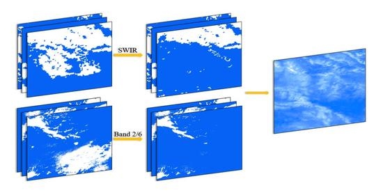
- SWIR Threshold Method
Cloud detection is done by essentially finding a threshold to most accurately distinguish between clear sky and cloudy pixels. Figure 2 shows the change of average reflectance values of four types of pixels of ice, snow, thin cloud, and thick cloud obtained at visible to short-wave infrared wavelengths. In true-color images, clouds that completely block ground objects are defined as thick clouds, and clouds that obscure ground objects are defined as thin clouds. The distinction between snow and ice is similar to the distinction between thick and thin clouds. These four types of pixels were selected from true-color images by visual interpretation in 2001, 2005, 2009, 2013, and 2016. These four types of pixels cover areas of different latitudes, elevations, and land cover. The number of samples of one type of pixel in a year is about 70~80. Since it is difficult to distinguish snow and cloud effectively through human eyes in winter at high latitudes, sample selection is subjective to some extent. In Figure 2, the spectral range from left to right represents band 8, band 9, band 3, band 4, band 1, band 2, band 5, band 6, and band 7 of MOD09GA, respectively. Band 2 is the near-infrared (NIR) band, Bands 5, 6, and 7 are short-wave infrared (SWIR) bands, and the rest are of the visible (VIS) spectrum. It can be seen that there is not much difference in the VIS between the reflectance values of thick clouds and snow, as well as between ice and thin clouds. However, the reflectance of snow and ice drops sharply at the NIR and SWIR, which differs greatly from that of thick and thin clouds. In the spectral range of 2105 nm to 2155 nm, the reflectance of snow and ice decreased to the lowest value. Ice and snow generally show a high degree of reflection in the VIS (wavelength ca 400~750 nm), lower reflection in the NIR (wavelength ca 780~900 nm), and very low reflection in the SWIR (wavelength ca 1570~1780 nm). Therefore, due to the coupled effects of the strong absorption by snow and ice in the SWIR, and the high reflection of clouds in the SWIR [47,48,49,50,51,52], we can use MODIS band 7 to perform threshold segmentation for snow, ice, and cloud, as shown in Equation (1).
In general, all kinds of clouds should have Band 7 reflectance larger than 0.03, referring to the LEDAPS (The Landsat Ecosystem Disturbance Adaptive Processing System) internal cloud masking algorithm. In this study, the threshold is set to 0.025 in order to prevent filtering out thin clouds. When the value of MODIS Band 7 is lower than 0.025, it should not be regarded as “cloudy”.
- Band 2/6 ratio threshold method
In addition to the confusion of snow and ice, and bright rocks and sand often appear in cloud masks, especially in desert areas. We can use the ratio of Band 2 to Band 6 to distinguish between clouds and sand, which is similar to the Band 4/5 ratio commonly used in Landsat to eliminate highly reflective sands and rocks [47,48]. Figure 3 exhibits the distribution of the ratios of Band 2 to Band 6 of cloud and sand, from which the sample points are taken from the true-color images by visual interpretation. The samples cover areas of bright sand and rocks at different latitudes and elevations in 2001, 2005, 2009, 2013, and 2016. The number of samples of one type of pixel in a year is about 300. The orange dots represent samples of thick and thin clouds, and the blue dots represent bright sand and rocks. The value of each dot represents the average of all pixels in the sample. The blue dots are less than approximately 0.85, and the orange dots are between 0.85 and 2. In principle, the sand and rocks tend to exhibit higher reflectance in Band 6 than that in Band 2, resulting in the ratio of Band 2 to Band 6 of sand usually being less than 1, whereas the reverse is true for clouds. However, sometimes the ratios of thin clouds are less than 1 due to the exposed sand and rock beneath thin clouds. As shown in Figure 3, the ratios of thin clouds are scattered between 0.85 and 1. The Band 2/6 test is shown in Equation (2).
2.2.2. Removal of Orbital Artifacts
The MODIS orbit results in systematic gaps in the daily global coverage near the equator that results in nearly longitudinal orbital artifacts (0° due north, approximately 15° for Terra, and 345° for Aqua) in the long-term cloud frequencies, as shown in Section 3.1. The orbital artifacts are evenly distributed in the MOD35 cloud mask between 180°W to 180°E and 30°S to 30°N. Such orbital artifacts are more pronounced at sea than on land. In the MOD09 cloud mask, orbital artifacts are not as obvious as in the MOD35 cloud mask, only visible in some areas. Therefore, in the MOD09 cloud mask, the orbital artifacts are visible over eastern Australia, northwest Africa, and South Asia. In addition, the absence of short-wave infrared in the winter at high latitudes has resulted in horizontal fringe noise in the Arctic areas. To remove these features, we used the Variational Stationary Noise Remover (VSNR) for the long-term cloud frequency data produced in part in 2.2.1 [39,53]. It can be interpreted both as a restoration method in a Bayesian framework and as a cartoon + texture decomposition method. The VSNR is able to preserve the image details and remove the stripes and most of the white noise. Therefore, it is well-suited to remove these artifacts by setting the shape, scale, and angle of known artifacts.
Images with obvious fringe noise were screened from 37 cloud frequency data (i.e., the year is broken down in 37 ten-day periods), and the problematic regions in these images were clipped as VSNR input data. The Gabor filter in VSNR was set to y = 200, x = 5, and θ = 15 for Terra and θ = –15 for Aqua to minimize the orbital artifacts in eastern Australia and the central Pacific areas. The Gabor filter with y = 40, x = 5, and θ = 15 for Terra and θ = –15 for Aqua was used in Northwest Africa and the northern Indian Ocean areas. The output image with the fringe noise removed is reinserted into the long-term cloud frequency data.
2.2.3. Removal of Abnormal Points
Examination of the resulting ten-day climatology revealed an abnormally high cloud frequency in some areas with high albedo and annual variability (SD), especially at the land-water junction. Although the MOD09 cloud mask performs much better than MOD35, the misclassification of clouds at the land/water interface is still obvious. Even the contours of land and water can clearly be seen depending on the distribution of clouds. Albedo from the 1 km MODIS MCD43B3 product was used to identify these problematic regions. These problematic areas generally fall into three categories: (1) land with high albedo and high variability (LAV), (2) water with high variability (WS), and (3) water with high albedo (WA). Therefore, MODIS MOD44W water mask products and SRTM Digital Elevation Data are employed to assist in identifying these areas. Equations (3)–(5), and (7) are the identification Equations for abnormal regions.
where, represents the minimum albedo of the pixel over 16 years. The slope is calculated from SRTM DEM. For , 0 and 1 represent a non-water surface and water surface, respectively. is the Coefficient of Variation (CV), which is obtained by Equation (6).
where, represents the standard deviation of the 16 years of albedo data, and represents the average of 16 years of albedo data.
The threshold setting of the above equation is referenced from the research by Wilson and Walter [39]. Therefore, through Equation (7), a binary image can be obtained to mask out the problem regions.
where, represents the areas with abnormal points.
The abnormal areas identified by this method are usually small areas such as narrow land and water boundaries. To avoid data loss after the deletion of abnormal areas, an interpolation method is used to fill these areas. The interpolation method may change the cloud frequency data of small regions, but it is ultimately more beneficial than harmful to remove abnormal regions in practical application. For example, an unusually high cloud frequency could lead to an inefficient location for a solar power station on water.
2.2.4. Quality Assessment Method
Due to the unfeasibility of obtaining precise simultaneous cloud information, the validation of a cloud product remains a challenging task. The available reference cloud products present their own inherent limitations and are often not as accurate as the products they are intended to evaluate. Given the implied lack of fully reliable datasets for cloud product validation, the quality assessment of a cloud product must be regarded as a product comparison rather than a product validation. The verification strategy in this article includes a direct validation and consistency check.
- Direct validation
Direct validation is a method to obtain the “relative truth value” on the pixel scale of the product by processing the ground observational data, to evaluate the accuracy of the remote sensing product by directly comparing observations with the remote sensing product. In the study by Wilson and Walter [39], monthly daytime ground-based cloud observations from 1997 to 2009 produced by Eastman and Warren [54] were used to validate their dataset from 2001 to 2015. The time difference between the ground-based cloud observations and the cloud dataset is huge both in terms of year span and daily observation time. To eliminate possible validation inaccuracies due to this large time difference, we used hourly data from ISD from 2001 to 2016. In this study, cloud observation data from the ISD were used to validate the 16-year average, ten-day cloud climatology. We extracted the hourly values of total clouds, which represent the percentage of the sky covered by all types of clouds at that time. The observations from 2001 to 2016 were collated to extract useful information (station ID, latitude and longitude, UTM time, and cloud record). The ground observations used to validate cloud products needed to meet three conditions. First, there should be at least one observational recorded between 0900 and 1500 local time to obtain the daily mean noon cloud frequency. Second, at least 6 out of every 10 days are observed to obtain the ten-day average cloud frequency. Third, observational data are available for at least 10 out of the 16 years to obtain the 16-year average ten-day cloud frequency. We relaxed the time conditions so that the remaining stations could be spread over as much of the world as possible. This time difference between satellite and ground observations affects the verification results to some extent. We filtered the stations that were available over the 37 time periods (i.e., the year was broken down into 37 ten-day periods), leaving 3777 stations.
To compare these observations with satellite data, it is important to consider that the sampling radius of these observations (the visible sky) depends on cloud height, cloud thickness, earth’s curvature, and other factors, but the range of an observation is usually much larger than a single 1 km MODIS pixel [39]. For this reason, we calculated the average of the GLHCC in a circle with a radius of 16 km [55] centered on each station, and converted the GLHCC into the average cloud cover within the sample radius, making it equivalent to the observed value of the station. Finally, regression analysis was conducted to obtain the correlation coefficient (R) and root mean square error (RMSE) of the two groups of data.
- Consistency check
Consistency check is a method of using the same type of remote sensing products with known accuracy to verify the remote sensing products tested. Consistency check helps to evaluate the consistency between different products, and can comprehensively reflect the relative accuracy of cloud products. In this study, a visual comparison and correlation analysis were conducted between the GLHCC, MOD/MYD35 [41], and PATMOS-X [56] to analyze the advantages and disadvantages of the regions with differences between them. Through the regression analysis of the GLHCC, MOD/MYD35, PATMOS-X, and observational data, the correlation coefficient and standard error are calculated, and the relative accuracy of the three is analyzed.
3. Results and Quality Assessment
3.1. Results
After the modification of the cloud mask and the production and improvement of products mentioned in Section 2, the 16-year average cloud climatology data for 37 time periods (i.e., the year is broken down into 37 ten-day periods) are finally obtained. Figure 4 is an example diagram of ten-day land cloud frequency, which shows a non-global region due to the absence of Band 7 at high latitudes in winter. In specific data sets, cloud frequency data for high latitude areas in summer are available. From left to right and from top to bottom, the graph shows the 2nd, 5th, 8th, 11th, 14th, 17th, 20th, 23rd, 26th, 29th, 32nd, and 35th ten-day period of the year, respectively.
Figure 5 shows the average of the 37 images (annual mean cloud frequency). The statistical results of cloud distribution on the land, except the poles, show that the annual average cloud cover is about 50.4%. The mean annual cloud frequency confirms equatorial South America, the Congo River basin in Africa, and Southeast Asia to be the cloudiest regions of the world, with annual cloud frequencies (proportion of days with a positive cloud flag) ≥ 80%. The Sahara Desert and the Middle East are the least cloudy areas with annual cloud frequencies ≤ 10%. Figure 6 is a histogram of the global land average cloud frequency across the 37 periods. It can be seen from the graph that the global cloud cover changes in a wavy pattern, with higher cloud frequencies in October, November, December, and January, and lower frequencies in June and July.
Regions also vary strongly in the temporal variability of cloud cover, both within and between years, as shown in Figure 7. The largest inter-annual variability (standard deviation over 16 years of the mean cloud frequency for each individual 10-day period) outside Antarctica occurs in the tropical and subtropical savannas and the shrublands (SD 18%). The regions with large intra-annual variability (16-year mean of the annual standard deviation over all 37 ten-day periods for every individual year) are mainly distributed in the tropical monsoon climate zones of South Asia and Southeast Asia and savanna climate zones in Africa, South America (SD 35%). However, the inter-annual and intra-annual variations of tropical desert climate are relatively small (SD 5%).
In the specific experiment process, to prove the reliability of the research, we have done comparative experiments focusing on many aspects. Taking the annual average cloud frequency over a region of East Asia in 2001 as an example, Collection 5 and Collection 6 of the MOD09 and MOD35 cloud masks were compared visually, as shown in Figure 8. From left to right and top to bottom, the images are Collection 5 of the MOD09 cloud mask, Collection 6 of the MOD09 cloud mask, Collection 5 of the MOD35 cloud mask, and Collection 6 of the MOD35 cloud mask. By visual comparison, Collection 6 of MOD09 shows more anomalies, with areas of unusually high cloud frequency consistent with city and water locations. This may be due to cloud mask algorithms misclassifying bright areas as clouds, regardless of whether the brightness is caused by bright buildings, bright land, or aerosols. Collection 5 of the MOD35 cloud mask exhibits similar problems as Collection 6 of MOD09 does in urban areas. Compared with Collection 5 of MOD35, Collection 6 has less abrupt cloud variation between different land covers. However, this does not mean that the bias of land cover and processing path in Collection 6 of MOD35 have been completely eliminated. We can find from the four figures that the cloud frequency of MOD35 is higher than that of MOD09 on the whole, especially in the northern part of China. In fact, northern China receives much less rainfall than southern China, which is not reflected in MOD35.
Therefore, we performed a visual examination of four cloud masks (Figure 9 and Figure 10). Figure 9 is the true-color image of East Asia on 3 February 2002, and Figure 10 shows cloud masks of Collection 5 (a) and 6 (b) of MOD09 and Collection 5 (c) and 6 (d) of MOD35 on 3 February 2002. Collection 6 (Figure 10b) of the MOD09 cloud mask identifies all bright areas that overlap with cities and water areas as clouds, which are still “clear” on Collection 5 of MOD09 (Figure 10a). Both Collection 5 (Figure 10c) and Collection 6 (Figure 10d) MOD35 cloud masks divide large areas of land with sparse vegetation or aerosols in winter into clouds. This may be the reason why cloud frequency based on the MOD35 cloud mask is higher than the cloud frequency based on the MOD09 cloud mask in northern China. In addition, all four identified clouds in the intertidal zone. This phenomenon is evident in Collection 6 of MOD09, Collection 5 of MOD35, and Collection 6 MOD35, probably due to the bright sand and reefs in the intertidal zone.
Overall, Collection 5 of MOD09 has a better performance with smoother transitions between adjacent areas and has no abrupt changes between land and water.
To further prove the usability of Collection 5 of MOD09, we have done comparative experiments with Collection 6 of MOD35, as shown in Figure 11 and Figure 12. Figure 11 shows the annual mean cloud frequency of Taihu Lake in China in 2001, located in the southern plain area. Strangely, the MOD35 cloud mask (Figure 11) shows extremely low cloud frequency over the lake without the influence of topography. Figure 12 shows the annual average cloud frequency for a region of Santiago del Estero in 2010. Figure 12a shows an area of Santiago where woodland is mixed with cultivated land, some of which has been left bare for years without crops. Figure 12b,c show the cloud frequency of the MOD09 and MOD35 cloud masks, respectively. The cloud frequency displayed by the MOD35 cloud mask shows a high degree of consistency with the land cover. It can be seen that the MOD35 cloud mask is severely affected by land cover and processing paths.
Based on the above comparison, this study finally identified Collection 5 of the MOD09 cloud mask as the most suitable data source for multi-year cloud frequency calculations.
The improvement of the MOD09 cloud mask is evidenced by the correction of snow, ice, and high reflectivity areas, which were otherwise misclassified as clouds. The error in the original MOD09 cloud mask will become more obvious with the average of multiple images. Figure 13a shows the first 16-year ten-day average cloud frequency based on the uncorrected MOD09 cloud mask in GLHCC01. It is unreasonable that the cloud frequency over Qinghai Lake and Hala Lake in winter is abnormally higher than the surrounding areas; and that the boundary between land and water is unusually clear. GLHCC01 represents the image of the first time period among the 37 time periods (i.e., the year is broken down into 37 ten-day periods), i.e., the average cloud frequency from 1 January to 10 January. It is caused by the mistaken classification of snow and ice in Qinghai Lake and Hala Lake in winter as clouds over many years. Taking Qinghai Lake on 6 January 2001 as an example, the correction effect of the SWIR threshold method on the MOD09 cloud mask is illustrated (Figure 14). Figure 14a is the true-color image of Qinghai Lake, from which it can be found that the reflectivity of ice, snow, and clouds on Qinghai Lake is extremely high. According to the characteristics of cloud distribution, shape, and cloud shadow, it can be ascertained that the highlighted areas on the lake surface are probably ice and snow rather than clouds. We can test our idea in the SWIR band. It can be seen from Figure 14b that part of the lake with high reflectivity originally within the range of VIS now presents low reflectivity within the range of SWIR, while some areas still have high reflectivity. This is because clouds are still highly reflective in short-wave infrared wavelengths, whereas snow and ice have low reflectivity because of the absorption of short-wave infrared wavelengths. Figure 14c,d show cloud masks before and after the correction of the SWIR threshold, respectively. The threshold here is set to 0.025 to prevent the thin cloud from being removed altogether. Figure 13b shows the average cloud frequency in GLHCC01 based on the corrected MOD09 cloud mask. Although the modified cloud frequency over Qinghai Lake and Hala Lake is still slightly higher than the surrounding area, there is a notable improvement. Figure 13c shows the effect after the treatment of the removal of the albedo anomaly, upon which the obvious land–water boundary is removed.
Taking the Sahara Desert in Northern Africa on 1 January 2008 as an example, the Band 2/6 ratio threshold method is used to separate particularly bright areas from the clouds, as shown in Figure 15. Figure 15a is a true-color image of an area in the Sahara showing the distribution of clouds. In the original GLHCC cloud mask shown in Figure 15c, it can be seen that a large bright area is mistakenly divided into clouds. This is because clouds, along with some bright rocks and sand, have high reflectivity at visible wavelengths. The ratio of Band 2 to Band 6 in Figure 15b can effectively distinguish clouds from bright rocks and sand because bright rock and desert tend to exhibit higher reflectance in Band 6 than in Band 2. Therefore, areas with a ratio greater than 1 are generally regarded as clouds; however, the threshold ratio is lowered to 0.85 to prevent the removal of some thin clouds. Figure 15d is the cloud mask modified by the Band 2/6 ratio threshold method for the MOD09 cloud mask, upon which non-clouded “cloudy” pixels are modified to “clear”.
The MODIS orbit causes systematic gaps in the daily global coverage near the equator, resulting in nearly longitudinal orbital artifacts (0° due north, approximately 15° for Terra and 345° for Aqua) for the long-term cloud frequencies. Figure 16 shows the comparison of the east coast of Australia before and after removing fringe noise in GLHCC01. To clearly show the elimination effect of fringe noise, we added the ocean area with more obvious noise. As shown in Figure 16a, there are several longitudinal stripes, of approximately 15°, at the point of the red arrow. The VSNR was adopted to eliminate these stripes, whose results after elimination were shown in Figure 16b. It can be seen that this technology can eliminate the fringe well and keep the image value close to the original value to ensure the accuracy of data. In this experiment, we set the x, y, and θ of the Gabor filter to 5, 200, and 15, respectively.
The observed cloud products reveal that the cloud frequency is unusually high in areas with a high albedo and annual variability (SD), especially at land–water intersections. The albedo from the 1 km MODIS MCD43B3 product and other data was used to identify these problematic regions. Using an example from the east coast of Africa in GLHCC01, we demonstrated the elimination effect of abnormal values (Figure 17). In order to clearly show the removal effect of abnormal areas, we retained the cloud frequency of the ocean area. As can be seen from Figure 17a, along the east coast of Africa there is a distinct white curve at the point of the red arrow, representing an abnormally high cloud frequency. These abnormal areas can be effectively identified and removed by the albedo anomaly removal method, and then be filled by interpolation. The effect after filling is shown in Figure 17b.
3.2. Quality Assessment
3.2.1. Direct Validation
In direct validation, we have compiled total cloud cover records from 3777 observation stations around the world for over 16 years to verify the cloud products of this study. Figure 18 shows the global distribution of weather stations used for verification. The northern hemisphere retains more weather stations than the southern hemisphere. The available observational data in parts of Africa and South America that meet the verification conditions are sparse or even absent in some places. Therefore, the validation result is affected by the uneven distribution of the observation data.
Figure 19 shows the global land average cloud frequency changes for the 37 time periods (i.e., the year broken is down in 37 ten-day periods) of ground observation data and the GLHCC. The “global” here refers to the areas covered by 3777 stations. Figure 19 shows that the frequency change trends of the two types of clouds are roughly the same, which are highly correlated. The observed cloud frequency is 1% to 5% higher than that of GLHCC products as a whole, which may be related to the observation and statistical methods of the two. Both types of data have higher average cloud frequencies in November, December, and January, and lower cloud frequencies in July, August, and September. Table 1 shows the specific values for comparison and validation of the two types of products over 37 time periods. The results show that the cloud products obtained in this study have a strong correlation with the observational data of meteorological stations. The average R of the verification results in 37 periods is 0.872 (Time 12: 0.8034~Time 30: 0.9105), and the RMSE is 9.3109 (Time 30: 7.9898~Time 19: 11.0265). In general, in October, November, and December, the GLHCC cloud products express the best degree of matching to the observation data. The correlation between the two is the smallest in April and May.
3.2.2. Consistency Check
In this study, PATMOS-X daily cloud data from 2010, with a resolution of 11 km, was selected as the consistency check comparison product. At the same time, in order to compare the advantages and disadvantages of different products, we added the annual average cloud frequency in 2010 based on the MOD/MYD35 cloud mask. Visual comparison and correlation analysis were conducted between GLHCC, MOD/MYD35, and PATMOS-X to analyze the relative merit of the regions with differences between them.
Figure 20 shows the global land average cloud frequency of the GLHCC (Figure 20a), MOD/MYD35 (Figure 20b), and PATMOS-X (Figure 20c), in 2010, excluding the poles. According to the statistics, the annual mean cloud frequencies over land, excluding polar regions, are 51.1%, 55.6%, and 52.8% for the GLHCC, MOD/MYD35, and PATMOS-X, respectively. The cloud frequency of MOD/MYD35 is significantly higher than that of the GLHCC and PATMOS-X in the middle and high latitudes of the Northern Hemisphere. Near the equator, the cloud frequency of PATMOS-X is significantly higher than GLHCC and MOD/MYD35. In addition, there are local differences in cloud frequency, mostly distributed in areas along a land-water boundary and regions with large terrain changes.
PATMOS-X has a much higher cloud frequency than the GLHCC and MOD/MYD35 on rivers and at the boundary of land and water, such as the coastline of Southeast Asia (Figure 21 and Figure 22) and the Amazon River Basin (Figure 23 and Figure 24). Figure 21 shows the cloud distribution of the GLHCC, MOD/MYD35, and PATMOS over southeast Asian islands in 2010. To show more clearly the cloud frequency along the island, the ocean area has been added here. Figure 21c shows an extremely anomalous land-water boundary in PATMOS-X, which is also observed near the equator in Africa and South America. In Figure 21a,b, the GLHCC and MOD/MYD35 show the opposite phenomenon to PATMOS-X; that is, the cloud frequency along the coast of the island is lower than the surrounding cloud frequency. This phenomenon is mainly due to the form of cloud distribution shown in Figure 22. At the boundary of land and sea, a long and narrow cloudless zone is formed due to the influence of topography, ocean currents, and other factors. Figure 23 is the cloud distribution of the GLHCC (Figure 23a), MOD/MYD35 (Figure 23b), and PATMOS-X (Figure 23c) over the Amazon River Basin. The GLHCC and MOD/MYD35 show lower cloud frequencies in the river region than in the surrounding region. However, PATMOS-X showed completely opposite results to the GLHCC and MOD/MYD35, with a higher cloud frequency over the river. By studying true-color images of the Amazon, it was determined that the cloud frequency of PATMOS-X was not consistent with the facts. Figure 24 shows an image of the Amazon on 1 June 2010, with cumulus clouds over the surrounding rainforest but not over the river. This phenomenon reveals transpiration in tropical rainforests, which is also common in tropical regions such as the Congo River Basin. This phenomenon is more obvious on MOD/MYD35 than in the GLHCC. It is difficult to determine which is more accurate, the GLHCC or MOD/MYD35. However, it is apparent that the river channel in the MOD35 cloud mask shows a very high cloud frequency, which is obviously inconsistent with the facts. The details are shown in an enlarged view in the lower right corner of Figure 23b, which is the area in the red box.
Cloud frequency has a strong relationship with topography in the regions with great undulating terrain, such as in the Eastern African region (Figure 25) and Western South America (Figure 26). Figure 25 shows the cloud frequency of East Africa in 2010 for the GLHCC (Figure 25a), MOD/MYD35 (Figure 25b), and PATMOS-X (Figure 25c). The cloud distributions of GLHCC and MOD/MYD35 over East Africa differ from that of PATMOS-X. In PATMOS-X, the cloud frequency over the Great Rift Valley is higher than that over the plateau region, while that over the coastal plain is lower than that over the plateau region. The lower cloud frequency for the Great Rift Valley in the GLHCC and MOD/MYD35 is more accurate than PATMOS-X because the Great Rift Valley is a typical dry-hot valley. In addition, the coastal plains and low foothills influenced by the tropical monsoon climate are wetter than the East African Plateau. Therefore, there is a high probability that the GLHCC and MOD/MYD35 are correct in their cloud estimation for this region. Figure 26 shows the cloud frequency of western South America in 2010 for the GLHCC (Figure 26a), MOD/MYD35 (Figure 26b), and PATMOS-X (Figure 26c). The GLHCC and MOD/MYD35 produce much higher cloud frequencies than PATMOS-X in the Andes Mountains. In the Southern Andes, the GLHCC showed a high cloud frequency, which was not seen in MOD/MYD35 or PATMOS-X. After investigation, it was found that the high cloud frequency displayed by the GLHCC in this area was mainly caused by the persistent snow cover throughout the year.
At the same time, we conducted regression analysis on the GLHCC, MOD/MYD35, PATMOS-X, and observed data, and the results are shown in Figure 27. The correlation coefficient (R) and Root Mean Square Errors (RMSE) of four cloud frequency data were obtained. Among them, the GHLCC and MOD/MYD35 obtained the largest R (0.9555) and the smallest RSME (4.5697%). PATMOS-X and the observations obtained the smallest R (0.7814) and the largest RSME (9.1718%). The R and RMSE of the GLHCC with observations and PATMOS-X were similar to those of MOD/MYD35 with observations and PATMOS-X. It can be seen that the GLHCC and MOD/MYD35 perform better, while PATMOS-X performs worst when the observations are taken as the truth value. In addition, the consistency between satellite data is higher than that between satellite data and observation data.
4. Discussion
The statistical results of cloud distribution on the land, except the poles, show that the annual average cloud cover is about 50.4%, which is slightly lower than the previous results of 52 to 56% of the annual average cloud cover over land [11,57,58]. To avoid the differences caused by different statistical regions, we calculated the cloud frequency of global land areas, except the poles, based on Collection 6 of the MOD35 cloud mask for 16 years, which is about 53.6%. At the same time, there was a nearly 4% difference in cloud frequencies between the GLHCC and MOD/MYD35 in 2010 (Section 3.2.2). There may be two main reasons for this result. First, the MOD09 cloud mask is only stored in one bit, a hybrid pixel with both “cloudy” and “clear” will be identified as “clear”. Therefore, the MOD09 cloud mask is not good at identifying thin clouds with very low optical thickness, and certainly does not misclassify aerosols as clouds (Figure 9 and Figure 10). Second, due to land cover deviation, the cloud cover of the MOD35 cloud mask is overestimated in some areas. Moreover, we found that the MOD35 cloud mask seems to be better at capturing objects with very low optical thickness (very thin clouds or aerosols) (Figure 9 and Figure 10). This sensitivity to objects with very low optical thickness is more useful for downstream product filtering data than for long-term cloud frequency calculations. As it is obviously unfair to classify such an object with extremely low optical thickness as a 100% cloud. The difference in attitude between the MOD09 and MOD35 cloud masks to-wards objects with very low optical thickness is also the reason for the difference in cloud frequency between them. In practical application, identifying the object with extremely low optical thickness as “Clear” is a better indicator of the true cloud distribution than identifying as a 100% cloud. Therefore, it can be argued that the MOD35 cloud mask is more suitable for downstream products, but the MOD09 cloud mask is more suitable for computing long-term cloud frequencies.
In the process of consistency check, the experiment well proves that the product cannot be evaluated from a single aspect. We choose which product to use based on the specific application, because each product has its advantages and disadvantages. The misestimation of cloud frequency in PATMOS-X was mainly reflected in the water surface, coastline, and mountainous areas. The abnormal cloud frequencies in MOD/MYD35 were mainly low cloud frequency over some water surfaces and high cloud frequency over exposed land surfaces (river channels, sparse grasslands, and cultivated land). The disadvantage of the GLHCC lies in its misjudgment of snow in high-altitude areas. The reason why this type of snow was not successfully removed by SWIR threshold method is that its reflectivity in short-wave infrared band is higher than the conservative SWIR threshold. This error occurs only at very high elevations, such as the Andes and Himalayas. Compared with the large area of misestimation by MOD/MYD35 and PATMOS-X, the GLHCC has a smaller misjudgment area. The advantages of the GLHCC products mainly originate from the relatively accurate statistics of cloud amounts of the MOD09 cloud mask. Although each product has its own advantages and disadvantages, on the whole, GLHCC can better represent the real situation of cloud frequency distribution.
5. Conclusions
In this study, the MOD09 cloud mask was improved by using a short-wave infrared threshold method and a Band 2/6 threshold method. The global 16-year average ten-day cloud frequency with a resolution of 1 km was produced based on the improved cloud mask and improved by VSNR and albedo products. The accuracy of the final GLHCC product was assessed by ground observations, MOD/MYD35 and PATMOS-X cloud data.
The short-wave infrared threshold method and Band 2/6 threshold method can effectively reduce the confusion of snow and ice, high brightness regions, and clouds in the GLHCC cloud mask. VSNR can effectively remove the orbital artifacts in cloud products, and the removal of albedo anomalies makes the cloud frequency at the land and water interface more reasonable. These algorithms enable the GLHCC cloud mask and the final product to more accurately reflect the global cloud distribution.
In the quality assessment stage, the correlation and standard errors between cloud products and observed data in 37 time periods (i.e., the year is broken down into 37 ten-day periods) were obtained by direct verification. The cloud products in 37 time periods exhibit a strong correlation with the observed data along with reasonable RMSE. A consistency check showed that the cloud frequency of GLHCC was lower than that of MOD/MYD35 and PATMOS-X on the whole, but better than MOD/MYD35 and PATMOS-X concerning the details. By regression analysis, R and RMSE between the GLHCC, MOD/MYD35, PATMOS-X, and 2010 observation data were obtained. The GLHCC had the greatest correlation with MOD/MYD35 and the smallest RMSE, while PATMOS-X had the worst correlation with the observed data and the largest RMSE. When using observational data as truth values, the GLHCC and MOD/MYD35 performed similarly, both outperforming PATMOS-X.
The experiments and studies in this paper have proved the high accuracy and availability of GLHCC product data, but there are still some problems and deficiencies. Due to the huge amount of data and the difficulty of calculation, the single threshold in the algorithm cannot adapt to the uncertainties in the global region. In addition, our algorithm, operating based on the MOD09 cloud mask, only excludes the non-cloud pixels misclassified as clouds, and clouds misclassified as non-cloud pixels may be missed. Therefore, in future studies, the single threshold value will be promoted to the dynamic threshold value to obtain the best threshold segmentation boundary in the global scope. Moreover, the comprehensive use of various cloud masks should be considered to recognize cloud pixels globally. For example, by combining the MOD09 and MOD35 cloud mask, the advantages of both are integrated and the disadvantages are eliminated to produce a more accurate cloud climatology. The lack of cloud climatology data in ocean areas may be filled in with the improved MOD35 cloud masks or other cloud products.
Author Contributions
Investigation, S.Z.; Methodology, S.Z. and F.C.; Project administration, Y.M., F.C., Y.Q. and J.L.; Validation, S.Z., E.S. and W.Y.; Writing—original draft, S.Z.; Writing—review and editing, S.Z. and Y.M. All authors have read and agreed to the published version of the manuscript.
Funding
This research was funded by the Guangxi Innovation-driven Development Special Project (GuiKe-AA20302022) and the Strategic Priority Research Program of the Chinese Academy of Sciences (NO. XDA19070201).
Data Availability Statement
Not Applicable.
Acknowledgments
Special acknowledgements should be expressed to the China-Pakistan Joint Research Center on Earth Sciences and Asian Regional Cooperation Fund (project: High-resolution remote sensing data and application services for SCO countries).
Conflicts of Interest
The authors declare no conflict of interest.
References
- Ardanuy, P.E.; Stowe, L.L.; Gruber, A.; Weiss, M.; Long, C.S. Longwave cloud radiative forcing as determined from nimbus-7 observations. J. Clim. 1989, 2, 766–799. [Google Scholar] [CrossRef] [Green Version]
- Ramanathan, V.; Cess, R.D. Cloud-radiative forcing and climate: Results from the Earth radiation budget experiment. Science 1989, 243, 57–63. [Google Scholar] [CrossRef] [PubMed] [Green Version]
- Stephens, G.L.; Webster, P.J. Clouds and climate—Sensitivity of simple systems. J. Atmos. Sci. 1981, 38, 235–247. [Google Scholar] [CrossRef]
- Trenberth, K.E.; Fasullo, J.T.; Kiehl, J. Earth’s global energy budget. Bull. Am. Meteorol. Soc. 2009, 90, 311–324. [Google Scholar] [CrossRef]
- Fischer, D.T.; Still, C.J.; Williams, A.P. Significance of summer fog and overcast for drought stress and ecological functioning of coastal California endemic plant species. J. Biogeogr. 2009, 36, 783–799. [Google Scholar] [CrossRef]
- Goldsmith, G.R.; Matzke, N.J.; Dawson, T.E. The incidence and implications of clouds for cloud forest plant water relations. Ecol. Lett. 2012, 16, 307–314. [Google Scholar] [CrossRef]
- Liou, K.N. Influence of cirrus clouds on weather and climate processes—A global perspective. Mon. Weather Rev. 1986, 114, 1167–1199. [Google Scholar] [CrossRef]
- Sklenar, P.; Bendix, J.; Balslev, H. Cloud frequency correlates to plant species composition in the high Andes of Ecuador. Basic Appl. Ecol. 2008, 9, 504–5133. [Google Scholar] [CrossRef]
- WMO. Guide to Meteorological Instruments and Methods of Observation; Secretariat of the World Meteorological Organization: Geneva, Switzerland, 1983. [Google Scholar]
- Hahn, C.J.; Warren, S.G.; London, J. The effect of moonlight on observation of cloud cover at night, and application to cloud climatology. J. Clim. 1995, 8, 1429–1446. [Google Scholar] [CrossRef] [Green Version]
- Stubenrauch, C.J.; Rossow, W.B.; Kinne, S.; Ackerman, S.; Cesana, G.; Chepfer, H. Assessment of global cloud datasets from satellites: Project and database initiated by the GEWEX radiation panel. Bull. Am. Meteorol. Soc. 2013, 94, 1031–1049. [Google Scholar] [CrossRef]
- Heidinger, A.K.; Foster, M.J.; Walther, A.; Zhao, X.T. The pathfinder atmospheres-extended AVHRR climate dataset. Bull. Am. Meteorol. Soc. 2014, 95, 909–922. [Google Scholar] [CrossRef]
- Foster, M.J.; Heidinger, A. PATMOS-x: Results from a diurnally corrected 30-yr satellite cloud climatology. J. Clim. 2013, 26, 414–425. [Google Scholar] [CrossRef]
- Foster, M.J.; Heidinger, A.; Hiley, M.; Wanzong, S.; Botambekov, D. PATMOS-x cloud climate record trend sensitivity to reanalysis products. Remote Sens. 2016, 8, 424. [Google Scholar] [CrossRef] [Green Version]
- Karlsson, K.G.; Riihel, A.; Müller, R.; Meirink, J.F.; Sedlar, J.; Stengel, M. CLARA-A1: A cloud, albedo, and radiation dataset from 28 yr of global AVHRR data. Atmos. Chem Phys. 2013, 13, 5351–5367. [Google Scholar] [CrossRef] [Green Version]
- Karlsson, K.G.; Anttila, K.; Trentmann, J.; Stengel, M.; Meirink, J.F.; Devasthale, A. CLARA-A2: The second edition of the CM SAF cloud and radiation data record from 34 years of global AVHRR data. Atmos. Chem. Phys. 2017, 17, 5809–5828. [Google Scholar] [CrossRef] [Green Version]
- Schiffer, R.A.; Rossow, W.B. The International-Satellite-Cloud-Climatology-Project (ISCCP)—The 1st project of the world-climate-research-programme. Bull. Am. Meteorol. Soc. 1983, 64, 779–784. [Google Scholar] [CrossRef] [Green Version]
- Schiffer, R.A.; Rossow, W.B. ISCCP global radiance data set—A new resource for climate research. Bull. Am. Meteorol. Soc. 1985, 66, 1498–1505. [Google Scholar] [CrossRef] [Green Version]
- Rossow, W.B.; Schiffer, R.A. ISCCP cloud data products. Bull. Am. Meteorol. Soc. 1991, 72, 2–20. [Google Scholar] [CrossRef]
- Barnes, W.L.; Pagano, T.S.; Salomonson, V.V. Prelaunch characteristics of the Moderate Resolution Imaging Spectroradiometer (MODIS) on EOS-AM1. IEEE Trans. Geosci. Remote. Sens. 1998, 36, 1088–1100. [Google Scholar] [CrossRef] [Green Version]
- Diner, D.J.; Beckert, J.C.; Reilly, T.H.; Bruegge, C.J.; Conel, J.E.; Kahn, R.A.; Martonchik, J.V.; Ackerman, T.P.; Davies, R.; Gerstl, S.A.W. Multi-angle Imaging SpectroRadiometer (MISR)–Instrument description and experiment overview. IEEE Trans. Geosci. Remote Sens. 1998, 36, 1072–1087. [Google Scholar] [CrossRef]
- Lee, R.B.; Barkstrom, B.R.; Smith, G.L.; Cooper, J.E.; Crommelynck, D.A.H. The Clouds and the Earth’s Radiant Energy System (CERES) sensors and preflight calibration plans. J. Atmos. Ocean. Technol. 1996, 13, 300–313. [Google Scholar] [CrossRef]
- Yamaguchi, Y.; Kahle, A.B.; Tsu, H.; Kawakami, T.; Pniel, M. Overview of Advanced Spaceborne Thermal Emission and Reflection Radiometer (ASTER). IEEE Trans. Geosci. Remote Sens. 1998, 36, 1062–1071. [Google Scholar] [CrossRef] [Green Version]
- Vane, D.; Stephens, G.L. The CloudSat mission and the A-Train: A revolutionary approach to observing Earth’s atmosphere. In Proceedings of the 2008 IEEE Aerospace Conference, Big Sky, MT, USA, 1–8 March 2008. [Google Scholar]
- Stephens, G.L.; Vane, D.G.; Boain, R.J.; Mace, G.G.; Austin, R.T. The cloudsat mission and the a-train—A new dimension of space-based observations of clouds and precipitation. Bull. Am. Meteorol. Soc. 2002, 83, 1771–1790. [Google Scholar] [CrossRef] [Green Version]
- Calbo, J.; Sanchez-Lorenzo, A. Cloudiness climatology in the Iberian Peninsula from three global gridded datasets (ISCCP, CRU TS 2.1, ERA-40). Theor. Appl. Clim. 2009, 96, 105–115. [Google Scholar] [CrossRef]
- Tzallas, V.; Hatzianastassiou, N.; Benas, N.; Meirink, J.; Matsoukas, C.; Stackhouse, P. Evaluation of CLARA-A2 and ISCCP-H cloud cover climate data records over Europe with ECA&D ground-based measurements. Remote Sens. 2019, 11, 212. [Google Scholar]
- Heidinger, A.K.; Evan, A.T.; Foster, M.J.; Walther, A. A Naive Bayesian Cloud-Detection Scheme Derived from CALIPSO and Applied within PATMOS-x. J. Appl. Meteorol. Clim. 2012, 51, 1129–1144. [Google Scholar] [CrossRef]
- Nielsen, J.K.; Foster, M.; Heidinger, A. Tropical stratospheric cloud climatology from the PATMOS-x dataset: An assessment of convective contributions to stratospheric water. Geophys. Res. Lett. 2011, 38, 38. [Google Scholar] [CrossRef] [Green Version]
- Levinson, D.H.; Lawrimore, J.H. State of the climate in 2007. Bull. Am. Meteorol. Soc. 2008, 89, S1–S179. [Google Scholar] [CrossRef]
- Tang, W.J.; Yang, K.; Qin, J.; Li, X.; Niu, X.L. A 16-year dataset (2000–2015) of high-resolution (3 h, 10 km) global surface solar radiation. Earth Syst. Sci. Data 2019, 11, 1905–1915. [Google Scholar] [CrossRef] [Green Version]
- Sassen, K.; Wang, Z. Classifying clouds around the globe with the CloudSat radar: 1-year of results. Geophys. Res. Lett. 2008, 35, 35. [Google Scholar] [CrossRef]
- Houze, R.A. Orographic effects on precipitating clouds. Rev. Geophys. 2012, 50, 50. [Google Scholar] [CrossRef]
- Wilson, A.M.; Silander, J.A. Estimating uncertainty in daily weather interpolations: A Bayesian framework for developing climate surfaces. Int. J. Climatol. 2014, 34, 2573–2584. [Google Scholar] [CrossRef]
- Stengel, M.; Stapelberg, S.; Sus, O.; Finkensieper, S.; Würzler, B.; Philipp, D.; Hollmann, R.; Poulsen, C.; Christensen, M.; McGarragh, G. Cloud_cci advanced very high resolution radiometer post meridiem (AVHRR-PM) dataset version 3: 35-year climatology of global cloud and radiation properties. Earth Syst. Sci. Data 2020, 12, 41–60. [Google Scholar] [CrossRef] [Green Version]
- Stengel, M.; Stapelberg, S.; Sus, O.; Schlundt, C.; Poulsen, C.; Thomas, G.; Christensen, M.; Henken, C.C.; Preusker, R.; Fischer, J.; et al. Cloud property datasets retrieved from AVHRR, MODIS, AATSR and MERIS in the framework of the Cloud_cci project. Earth Syst. Sci. Data 2017, 9, 881–904. [Google Scholar] [CrossRef] [Green Version]
- Douglas, M.; Beida, R.; Dominguez, A. Developing high spatial resolution daytime cloud climatologies for Africa. In Proceedings of the Preprints, 29th Conference on Hurricanes and Tropical Meteorology, Tucson, AZ, USA, 13 May 2010. [Google Scholar]
- Descloitres, J.; Sohlberg, R.; Owens, J.; Giglio, L.; Justice, C.; Carroll, M.; Seaton, J.; Crisologo, M.; Finco, M.; Lannom, K. The MODIS rapid response project. In Proceedings of the IEEE International Geoscience and Remote Sensing Symposium, Toronto, ON, Canada, 24–28 June 2002; pp. 1191–1192. [Google Scholar]
- Wilson, A.M.; Jetz, W. Remotely sensed high-resolution global cloud dynamics for predicting ecosystem and biodiversity distributions. PLoS Biol. 2016, 14, e1002415. [Google Scholar] [CrossRef] [PubMed]
- Mulligan, M. MODIS MOD35 Pan-Tropical Cloud Climatology. Available online: http://www.ambiotek.com/clouds/ (accessed on 1 July 2021).
- Wilson, A.M.; Parmentier, B.; Jetz, W. Systematic land cover bias in Collection 5 MODIS cloud mask and derived products—A global overview. Remote Sens. Environ. 2014, 141, 149–154. [Google Scholar] [CrossRef]
- Frey, R.A.; Ackerman, S.A.; Liu, Y.; Strabala, K.I.; Zhang, H.; Key, J. Cloud detection with MODIS. Part I: Improvements in the MODIS cloud mask for collection 5. J. Atmos. Ocean. Technol. 2008, 25, 1057–1072. [Google Scholar] [CrossRef]
- Leinenkugel, P.; Kuenzer, C.; Dech, S. Comparison and enhancement of MODIS cloud mask products for Southeast Asia. Int. J. Remote Sens. 2013, 34, 2730–2748. [Google Scholar] [CrossRef]
- Petitcolin, F.; Vermote, E. Land surface reflectance, emissivity and temperature from MODIS middle and thermal infrared data. Remote Sens. Environ. 2002, 83, 112–134. [Google Scholar] [CrossRef]
- Roger, J.C.; Vermote, E.F. A method to retrieve the reflectivity signature at 3.75 μm from AVHRR data. Remote Sens. Environ. 1998, 64, 103–114. [Google Scholar] [CrossRef]
- Kalnay, E. The NCEP/NCAR 40-year reanalysis project. Bull. Am. Meteorol. Soc. 1996, 77, 437–471. [Google Scholar] [CrossRef] [Green Version]
- Irish, R.R. Landsat 7 automatic cloud cover assessment. In Proceedings of the SPIE: The International Society for Optical Engineering, Orlando, FL, USA, 24–26 April 2000; pp. 348–355. [Google Scholar]
- Zhu, Z.; Woodcock, C.E. Object-based cloud and cloud shadow detection in Landsat imagery. Remote Sens. Environ. 2012, 118, 83–94. [Google Scholar] [CrossRef]
- Chen, N.; Li, W.; Tanikawa, T.; Hori, M.; Aoki, T.; Stamnes, K. Cloud mask over snow-/ice-covered areas for the GCOM-C1/SGLI cryosphere mission: Validations over Greenland. J. Geophys. Res. Atmos. 2014, 119, 12287–12300. [Google Scholar] [CrossRef]
- Hall, D.K.; Riggs, G.A.; Salomonson, V.V. Development of methods for mapping global snow cover using moderate resolution imaging spectroradiometer data. Remote Sens. Environ. 1995, 54, 127–140. [Google Scholar] [CrossRef]
- Hutchison, K.D.; Mahoney, R.L.; Iisager, B.D. Discriminating sea ice from low-level water clouds in split-window, mid-wavelength IR imagery. Int. J. Remote Sens. 2013, 34, 7131–7144. [Google Scholar] [CrossRef]
- Liu, Y.H.; Ackerman, S.A.; Maddux, B.C.; Key, J.R.; Frey, R.A. Errors in cloud detection over the arctic using a satellite imager and implications for observing feedback mechanisms. J. Clim. 2010, 23, 1894–1907. [Google Scholar] [CrossRef] [Green Version]
- Fehrenbach, J.; Weiss, P.; Lorenzo, C. Variational algorithms to remove stationary noise: Applications to microscopy imaging. IEEE Trans. Image Process. 2012, 21, 4420–4430. [Google Scholar] [CrossRef] [PubMed] [Green Version]
- Eastman, R.; Warren, S.G. Land Cloud Update, 1997–2009, Appended to Cloud Climatology for Land Stations Worldwide, 1971–1996. Available online: http://cdiac.ornl.gov/epubs/ndp/ndp026d/ndp026d.html (accessed on 15 July 2021).
- Dybbroe, A.; Karlsson, K.G.; Thoss, A. NWCSAF AVHRR cloud detection and analysis using dynamic thresholds and radiative transfer modeling. Part II: Tuning and validation. J. Appl. Meteorol. 2005, 44, 55–71. [Google Scholar] [CrossRef]
- Heidinger, A.; Foster, M.; Botambekov, D.; Hiley, M.; Walther, A.; Li, Y. Using the NASA EOS A-train to probe the performance of the NOAA PATMOS-x Cloud Fraction CDR. Remote Sens. 2016, 8, 511. [Google Scholar] [CrossRef] [Green Version]
- King, M.D.; Platnick, S.; Menzel, W.P.; Ackerman, S.A.; Hubanks, P.A. Spatial and temporal distribution of clouds observed by MODIS onboard the Terra and Aqua satellites. IEEE Trans. Geosci. Remote 2013, 51, 3826–3852. [Google Scholar] [CrossRef]
- Pincus, R.; Platnick, S.; Ackerman, S.A.; Hemler, R.S.; Hofmann, R.J.P. Reconciling simulated and observed views of clouds: MODIS, ISCCP, and the limits of instrument simulators. J. Clim. 2012, 25, 4699–4720. [Google Scholar] [CrossRef]
Figure 1.
Flowchart for production and quality assessment of the GLHCC product.

Figure 2.
The variation of the reflectance of four types of pixels in different spectral ranges. See text for explanation.
Figure 2.
The variation of the reflectance of four types of pixels in different spectral ranges. See text for explanation.

Figure 3.
Distribution in the ratios of Band 2 to Band 6 of clouds and sand. See text for explanation.
Figure 3.
Distribution in the ratios of Band 2 to Band 6 of clouds and sand. See text for explanation.

Figure 4.
The 16-year ten-day average cloud frequency (%) for the 2nd (a), 5th (b), 8th (c), 11th (d), 14th (e), 17th (f), 20th (g), 23rd (h), 26th (i), 29th (j), 32nd (k), and 35th (l) ten-day period, respectively.
Figure 4.
The 16-year ten-day average cloud frequency (%) for the 2nd (a), 5th (b), 8th (c), 11th (d), 14th (e), 17th (f), 20th (g), 23rd (h), 26th (i), 29th (j), 32nd (k), and 35th (l) ten-day period, respectively.

Figure 5.
Mean annual cloud frequency (%) of the GLHCC.

Figure 6.
The global land average cloud frequency of GLHCC over 37 time periods (%).

Figure 7.
The inter-annual variability (a) and intra-annual variability (b) of cloud frequency.

Figure 8.
Annual mean cloud frequency (%) for 2001 based on Collection 5 (a) and 6 (b) of MOD09 cloud mask and Collection 5 (c) and 6 (d) of the MOD35 cloud mask. The red arrow points to the Yellow River.
Figure 8.
Annual mean cloud frequency (%) for 2001 based on Collection 5 (a) and 6 (b) of MOD09 cloud mask and Collection 5 (c) and 6 (d) of the MOD35 cloud mask. The red arrow points to the Yellow River.

Figure 9.
True-color image of East Asia on 3 February 2002.

Figure 10.
Cloud masks of Collection 5 (a) and 6 (b) of MOD09 and Collection 5 (c) and 6 (d) of MOD35 on 3 February 2002.
Figure 10.
Cloud masks of Collection 5 (a) and 6 (b) of MOD09 and Collection 5 (c) and 6 (d) of MOD35 on 3 February 2002.

Figure 11.
Annual mean cloud frequency (%) over Taihu Lake in 2001 based on Collection 5 of MOD09 cloud mask (a) and Collection 6 of MOD35 cloud mask (b).
Figure 11.
Annual mean cloud frequency (%) over Taihu Lake in 2001 based on Collection 5 of MOD09 cloud mask (a) and Collection 6 of MOD35 cloud mask (b).

Figure 12.
Cloud frequency of Santiago del Estero. (a) True-color image of the Santiago del Estero on 1 June 2010; (b) cloud frequency in 2010 based on the MOD09 cloud mask; (c) cloud frequency in 2010 based on the MOD35 cloud mask.
Figure 12.
Cloud frequency of Santiago del Estero. (a) True-color image of the Santiago del Estero on 1 June 2010; (b) cloud frequency in 2010 based on the MOD09 cloud mask; (c) cloud frequency in 2010 based on the MOD35 cloud mask.

Figure 13.
Cloud frequency (%) of Qinghai Lake and Hala Lake in GLHCC01. (a) Cloud frequency based on the uncorrected MOD09 cloud mask; (b) cloud frequency based on the corrected MOD09 cloud mask; (c) cloud frequency after the removal of the albedo anomaly.
Figure 13.
Cloud frequency (%) of Qinghai Lake and Hala Lake in GLHCC01. (a) Cloud frequency based on the uncorrected MOD09 cloud mask; (b) cloud frequency based on the corrected MOD09 cloud mask; (c) cloud frequency after the removal of the albedo anomaly.

Figure 14.
Correction effect of the SWIR threshold method. (a) True-color image of Qinghai Lake (Band 1, 4, 3) on 6 January 2001; (b) short-wave infrared image (Band 7); (c) uncorrected MOD09 cloud mask; (d) corrected MOD09 cloud mask.
Figure 14.
Correction effect of the SWIR threshold method. (a) True-color image of Qinghai Lake (Band 1, 4, 3) on 6 January 2001; (b) short-wave infrared image (Band 7); (c) uncorrected MOD09 cloud mask; (d) corrected MOD09 cloud mask.

Figure 15.
Correction effect of Band 2/6 ratio threshold method. (a) True-color image of Sahara Desert (band 1, 4, 3) on 1 January 2008; (b) the ratio of Band 2 and Band 6 image of Sahara Desert; (c) uncorrected MOD09 cloud mask; (d) corrected MOD09 cloud mask.
Figure 15.
Correction effect of Band 2/6 ratio threshold method. (a) True-color image of Sahara Desert (band 1, 4, 3) on 1 January 2008; (b) the ratio of Band 2 and Band 6 image of Sahara Desert; (c) uncorrected MOD09 cloud mask; (d) corrected MOD09 cloud mask.

Figure 16.
Comparison of stripe noise before (a) and after (b) removal on the east coast of Australia in GLHCC01. The red arrow points to the striped noise.
Figure 16.
Comparison of stripe noise before (a) and after (b) removal on the east coast of Australia in GLHCC01. The red arrow points to the striped noise.

Figure 17.
Comparison of the east coast of Africa before (a) and after (b) removal of the anomaly in the GLHCC01 cloud climatology. The red arrow points to the problem areas with abnormal cloud frequency.
Figure 17.
Comparison of the east coast of Africa before (a) and after (b) removal of the anomaly in the GLHCC01 cloud climatology. The red arrow points to the problem areas with abnormal cloud frequency.

Figure 18.
Global distribution of weather stations.

Figure 19.
Changes in global average cloud frequency (%) over 37 time periods of ground observation data and GLHCC products.
Figure 19.
Changes in global average cloud frequency (%) over 37 time periods of ground observation data and GLHCC products.

Figure 20.
Average global cloud frequency (%) of GLHCC (a), MOD/MYD35 (b), and PATMOS-X (c) in 2010.
Figure 20.
Average global cloud frequency (%) of GLHCC (a), MOD/MYD35 (b), and PATMOS-X (c) in 2010.

Figure 21.
Average cloud frequency (%) in the Southeast Asian Archipelago areas for the GLHCC (a), MOD/MYD35 (b), and PATMOS-X (c) in 2010.
Figure 21.
Average cloud frequency (%) in the Southeast Asian Archipelago areas for the GLHCC (a), MOD/MYD35 (b), and PATMOS-X (c) in 2010.

Figure 22.
The true-color images (band 1, 4, 3) of Sumatra on 8 June 2011 (a) and 1 June 2010 (b).

Figure 23.
Cloud frequency (%) of the Amazon in 2010 for the GLHCC (a), MOD/MYD35 (b), and PATMOS-X (c). The magnified image in the lower right corner of each image corresponds to the area of the red rectangle.
Figure 23.
Cloud frequency (%) of the Amazon in 2010 for the GLHCC (a), MOD/MYD35 (b), and PATMOS-X (c). The magnified image in the lower right corner of each image corresponds to the area of the red rectangle.

Figure 24.
The true-color image of the Amazon on 1 June 2010.

Figure 25.
Cloud frequency (%) of East Africa in 2010 of GLHCC (a), MOD/MYD35 (b), and PATMOS-X (c).
Figure 25.
Cloud frequency (%) of East Africa in 2010 of GLHCC (a), MOD/MYD35 (b), and PATMOS-X (c).

Figure 26.
Cloud frequency (%) of Western South America in 2010 for the GLHCC (a), MOD/MYD35 (b), and PATMOS-X (c).
Figure 26.
Cloud frequency (%) of Western South America in 2010 for the GLHCC (a), MOD/MYD35 (b), and PATMOS-X (c).

Figure 27.
Correlation analysis of the PATMOS-X (a), GLHCC (b–d), MOD/MYD35 (e,f) and observation data in 2010.
Figure 27.
Correlation analysis of the PATMOS-X (a), GLHCC (b–d), MOD/MYD35 (e,f) and observation data in 2010.


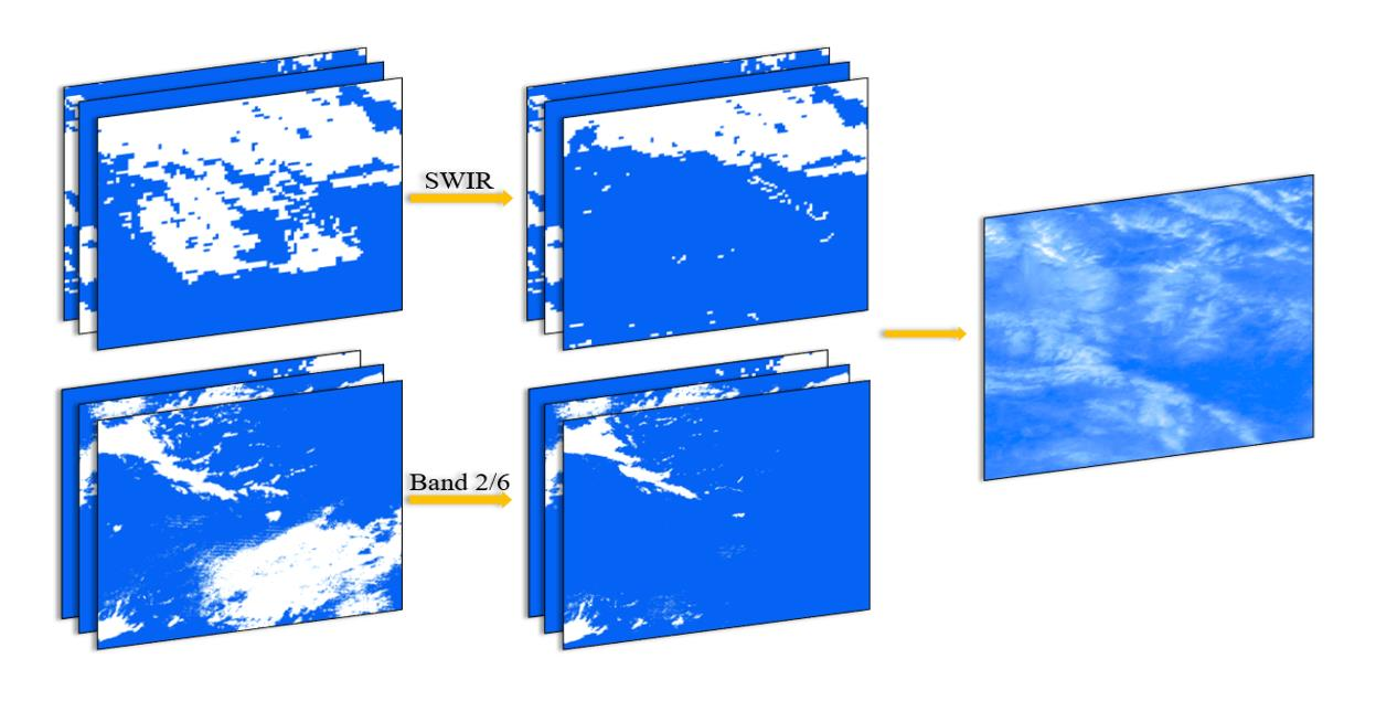
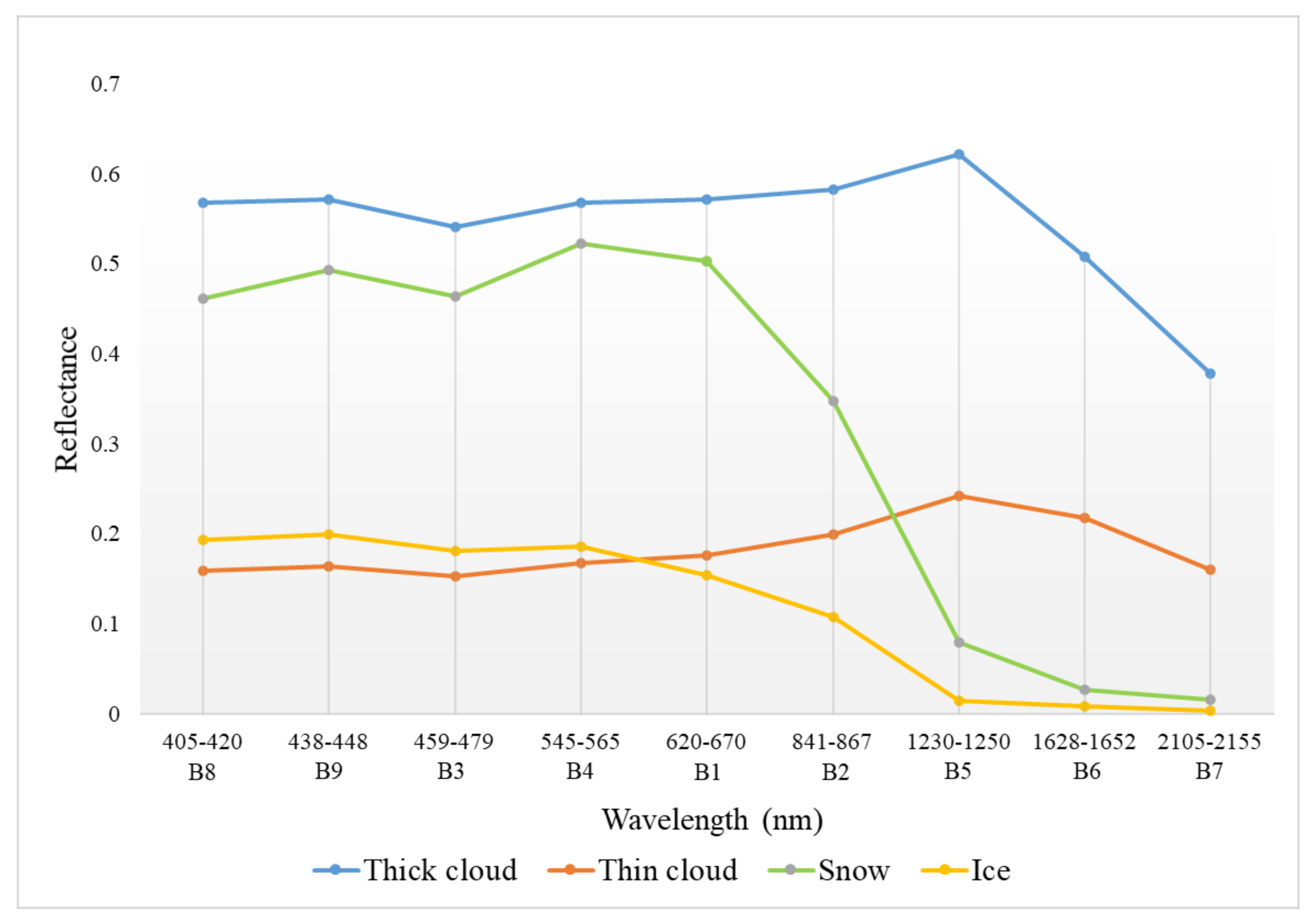
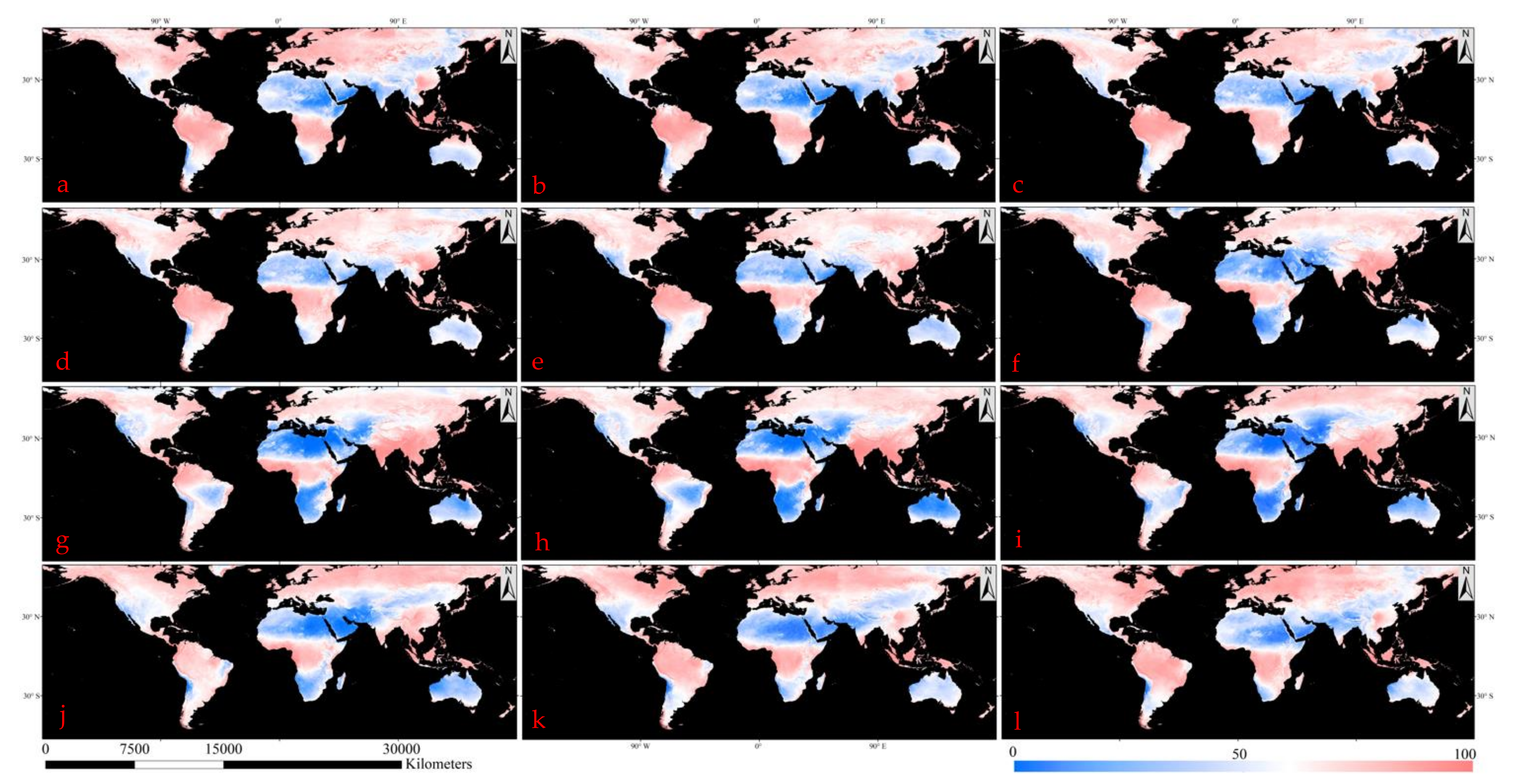
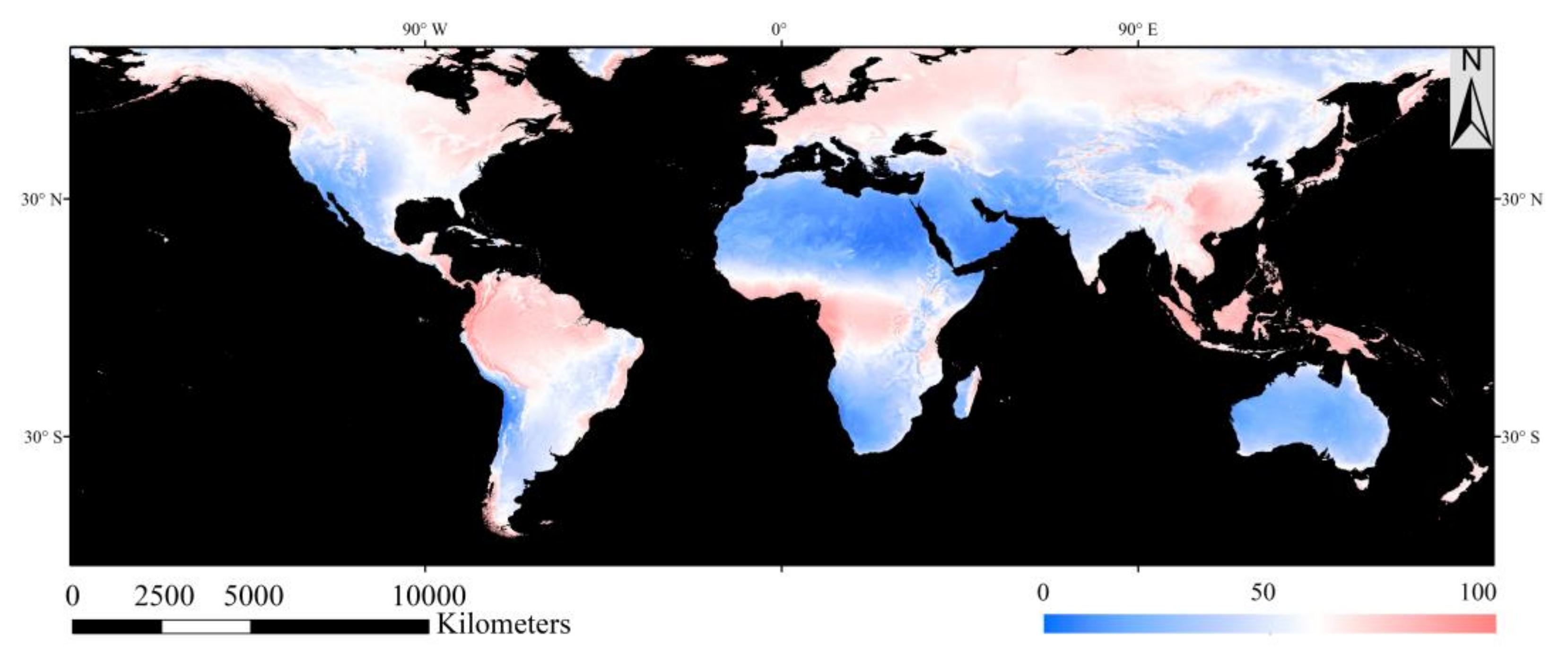
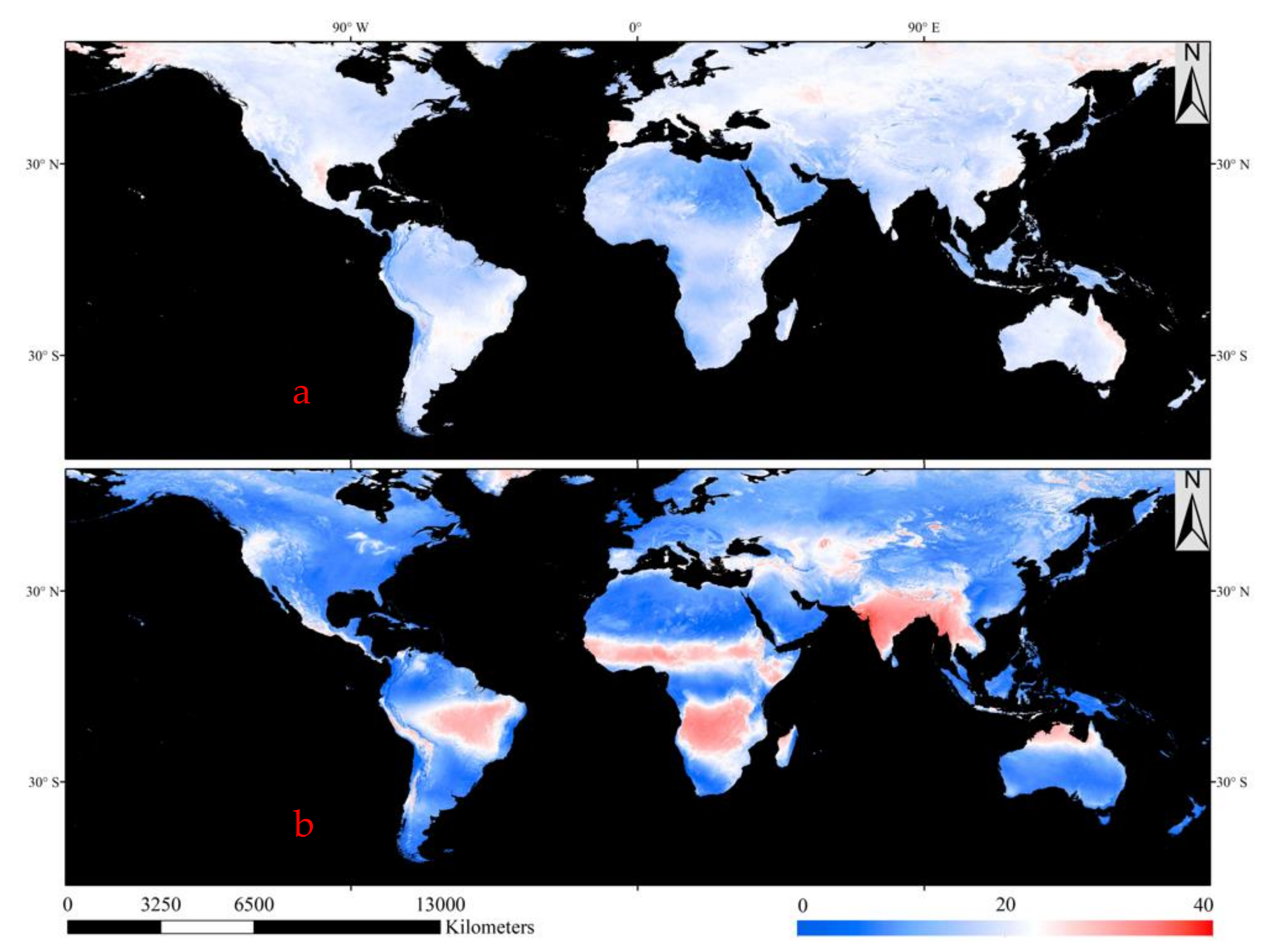
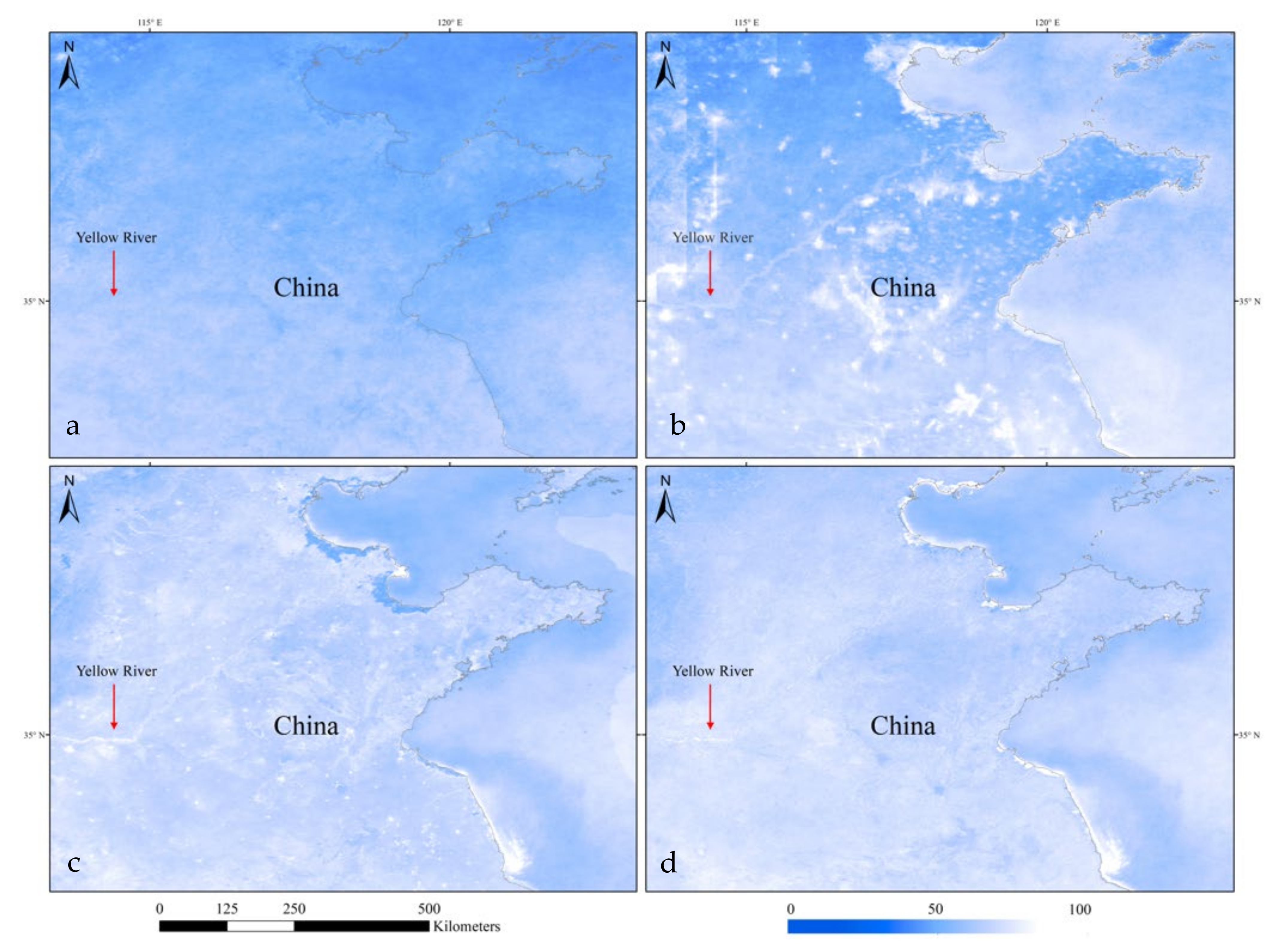
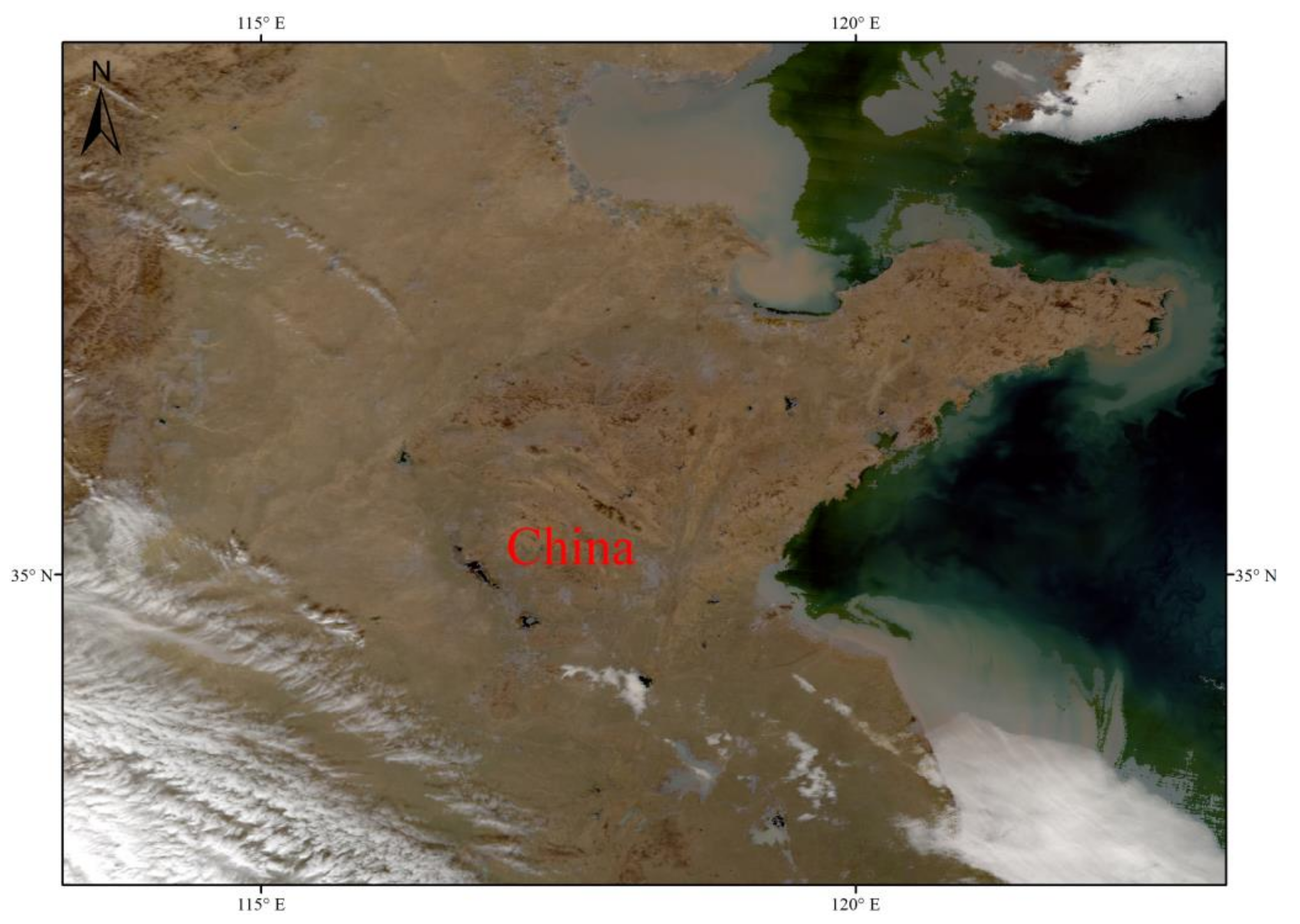
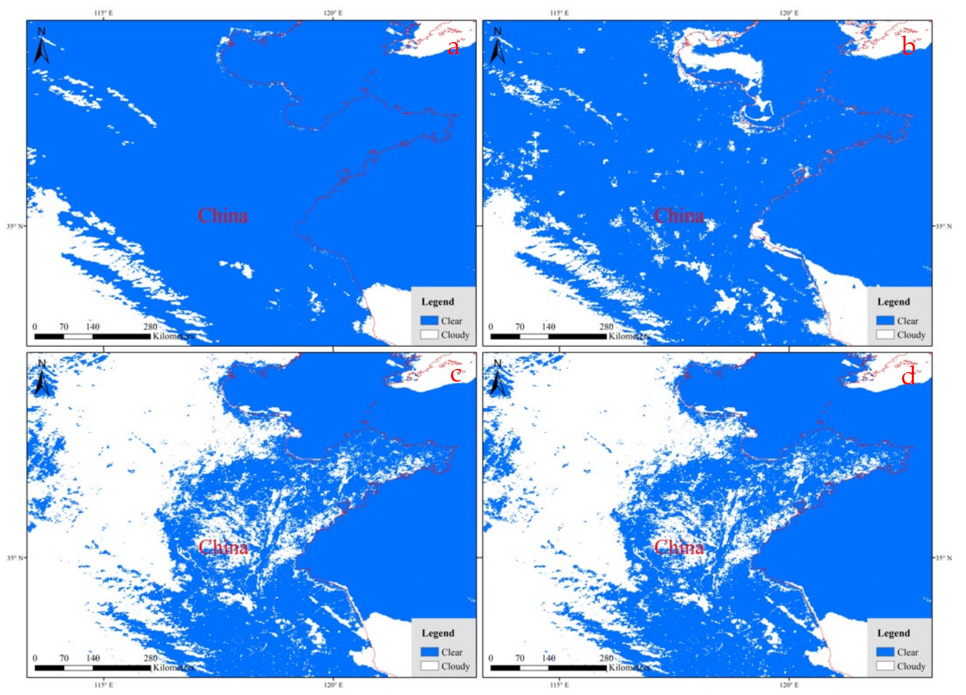
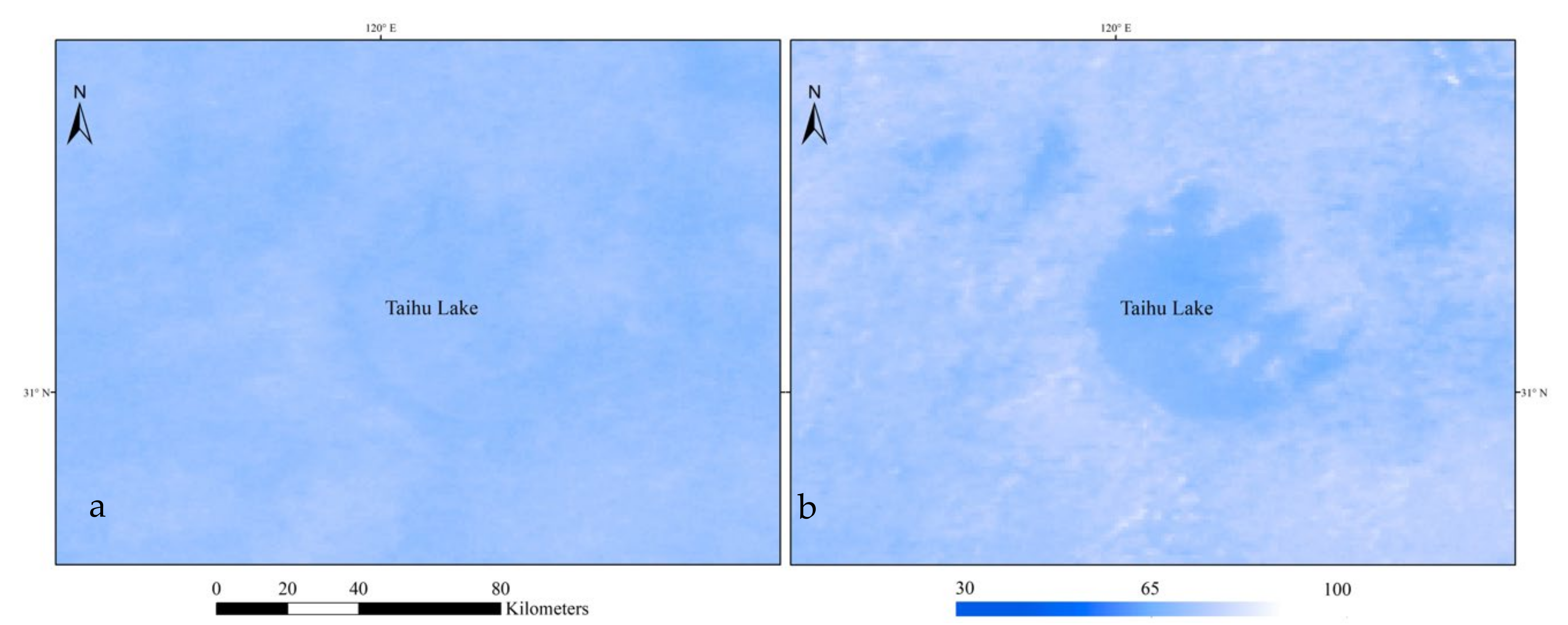
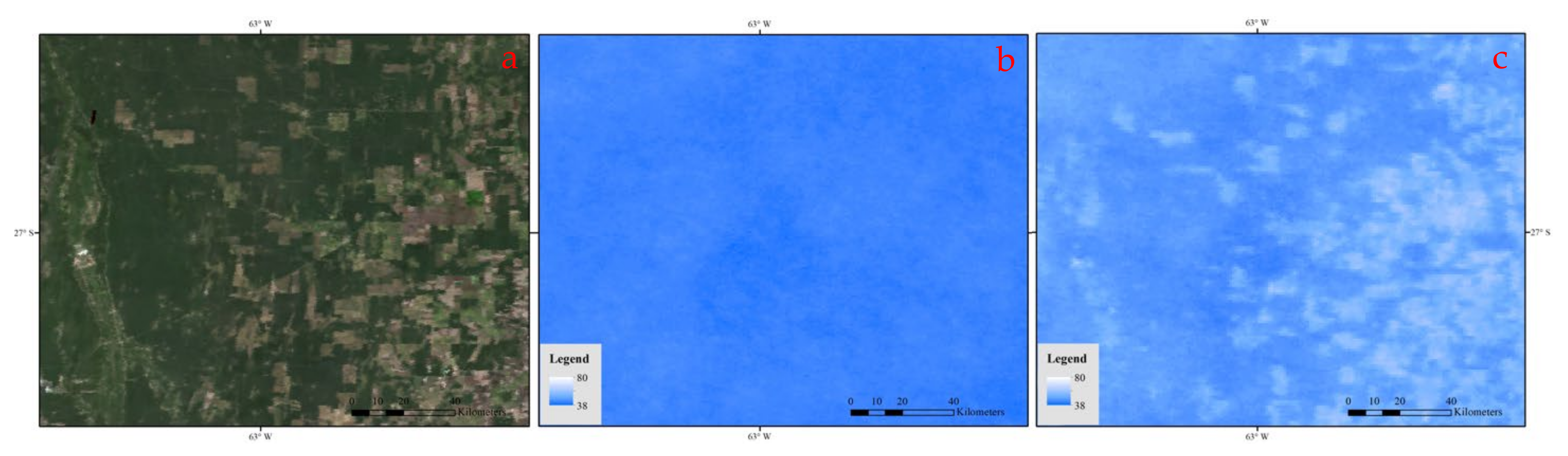
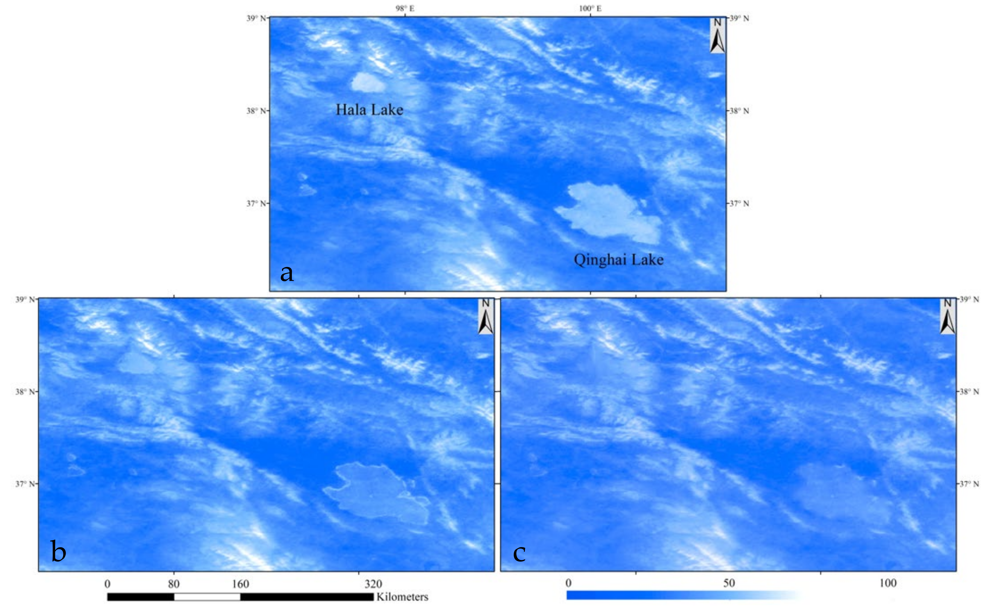
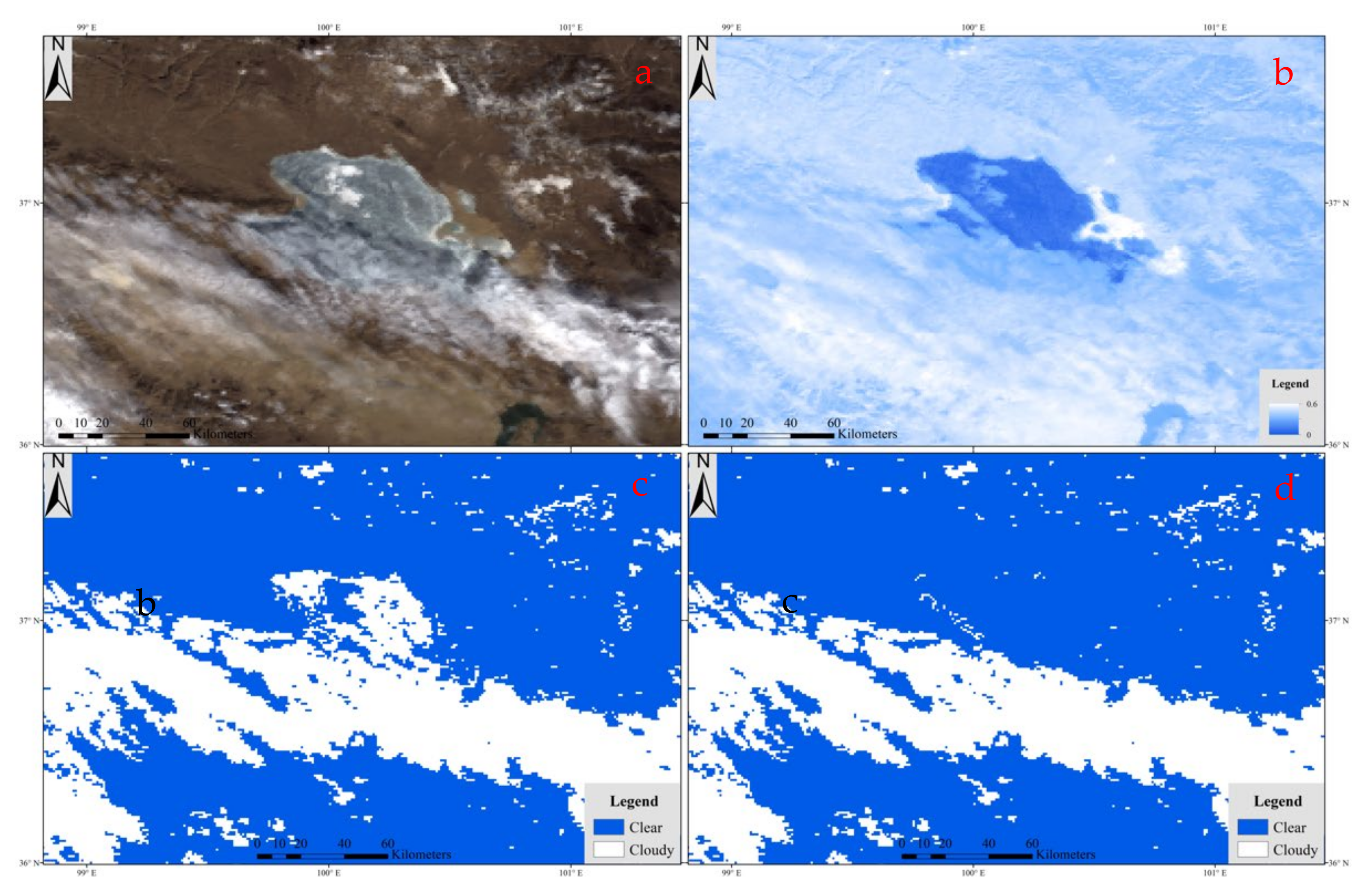
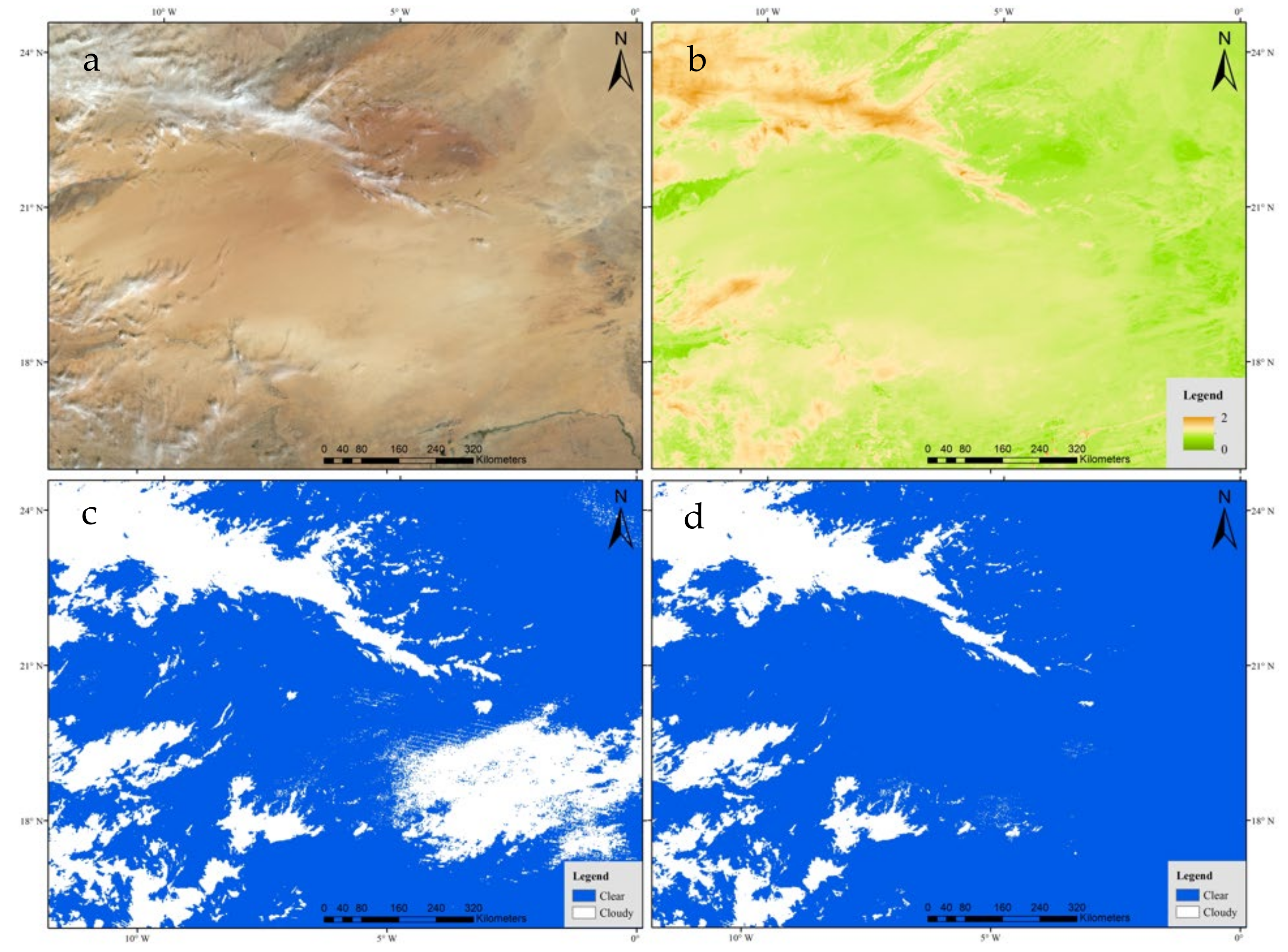
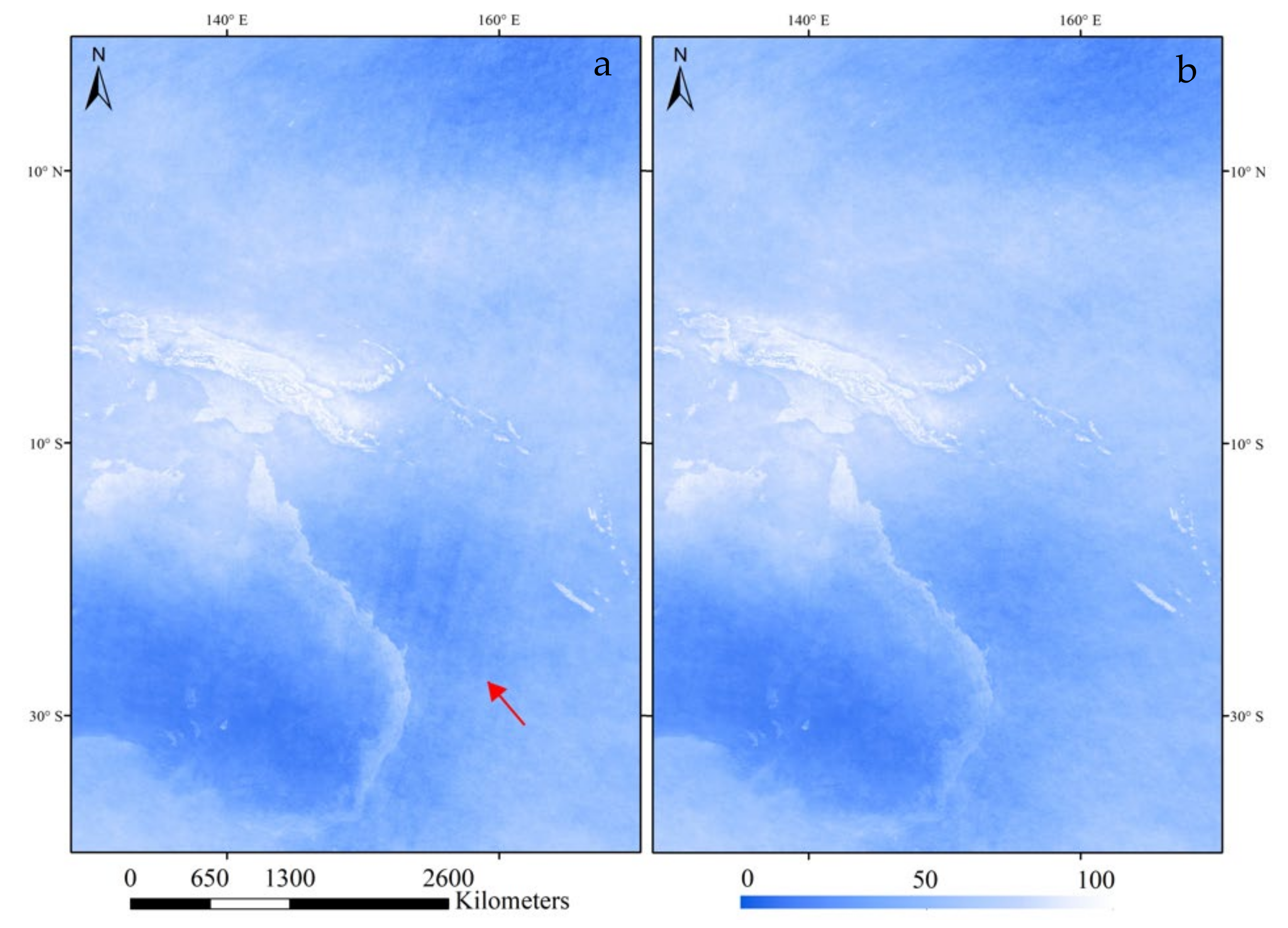
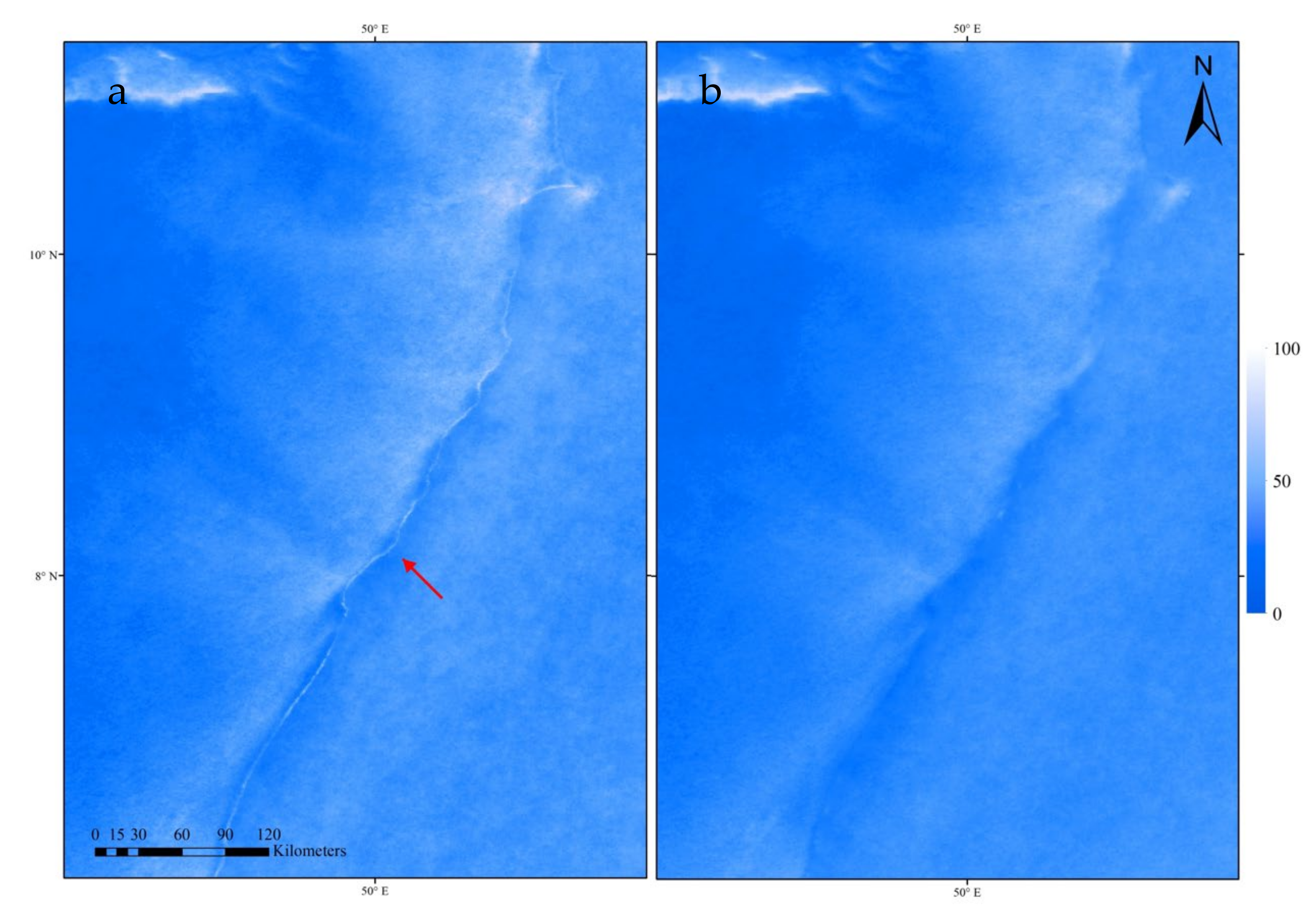
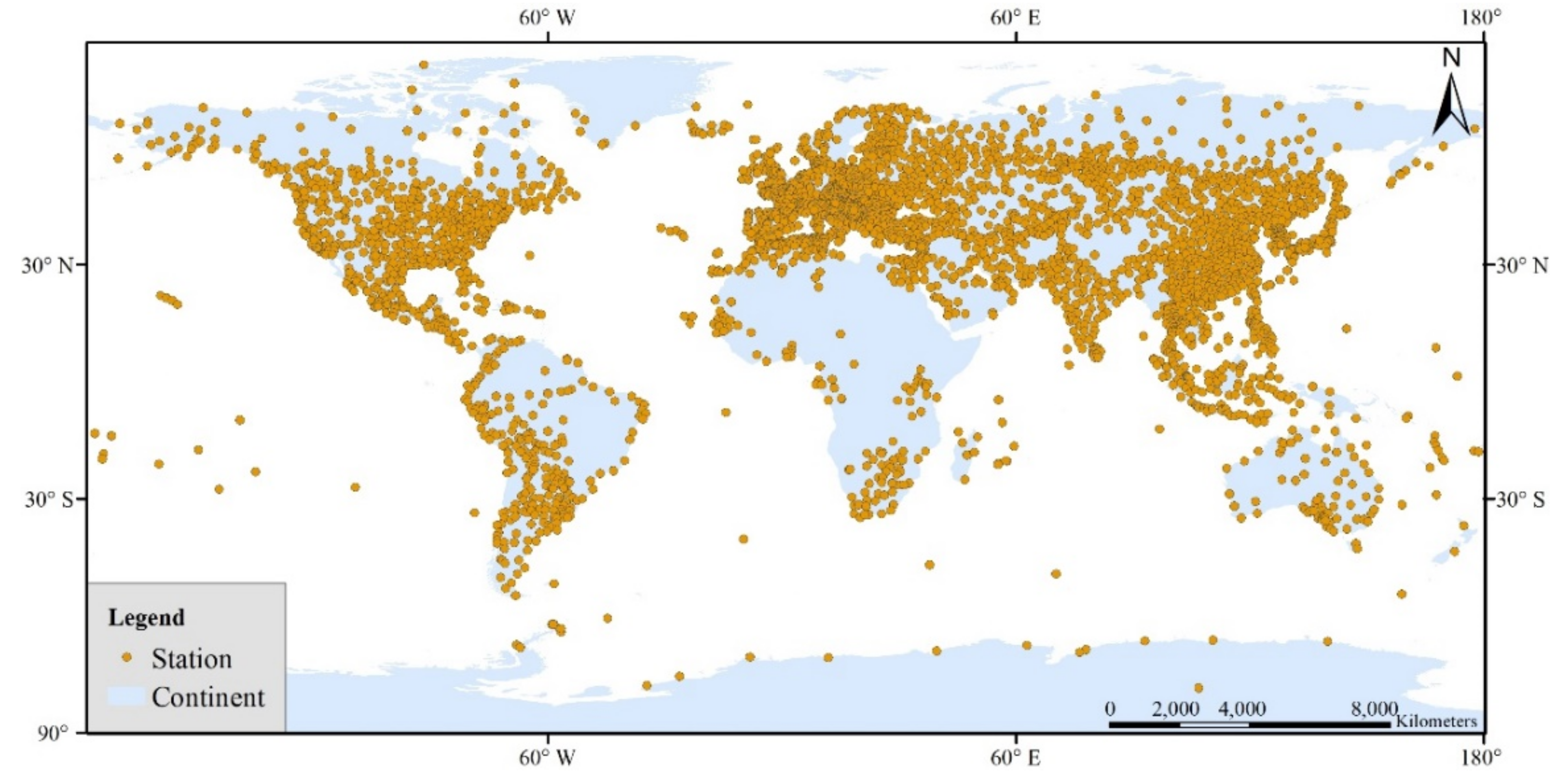
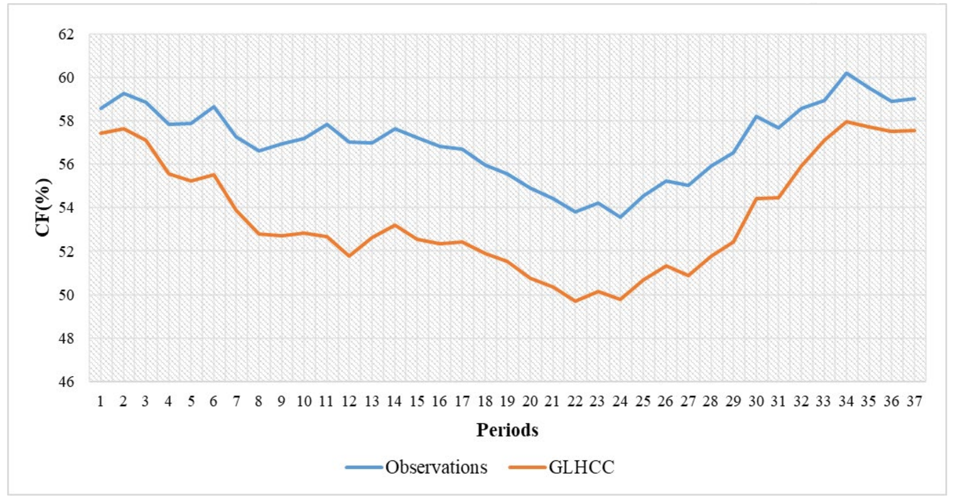
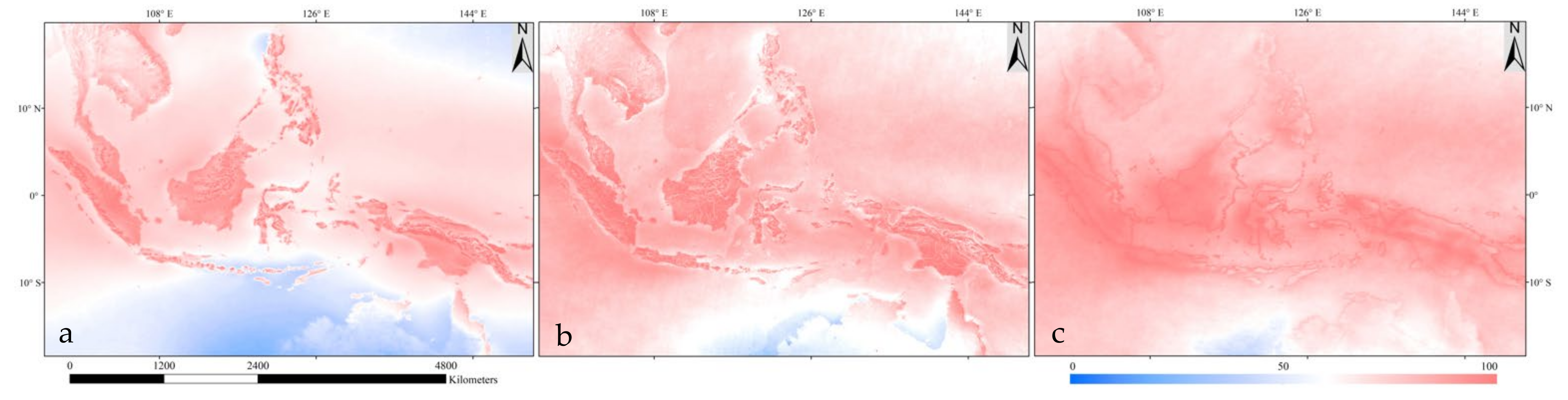
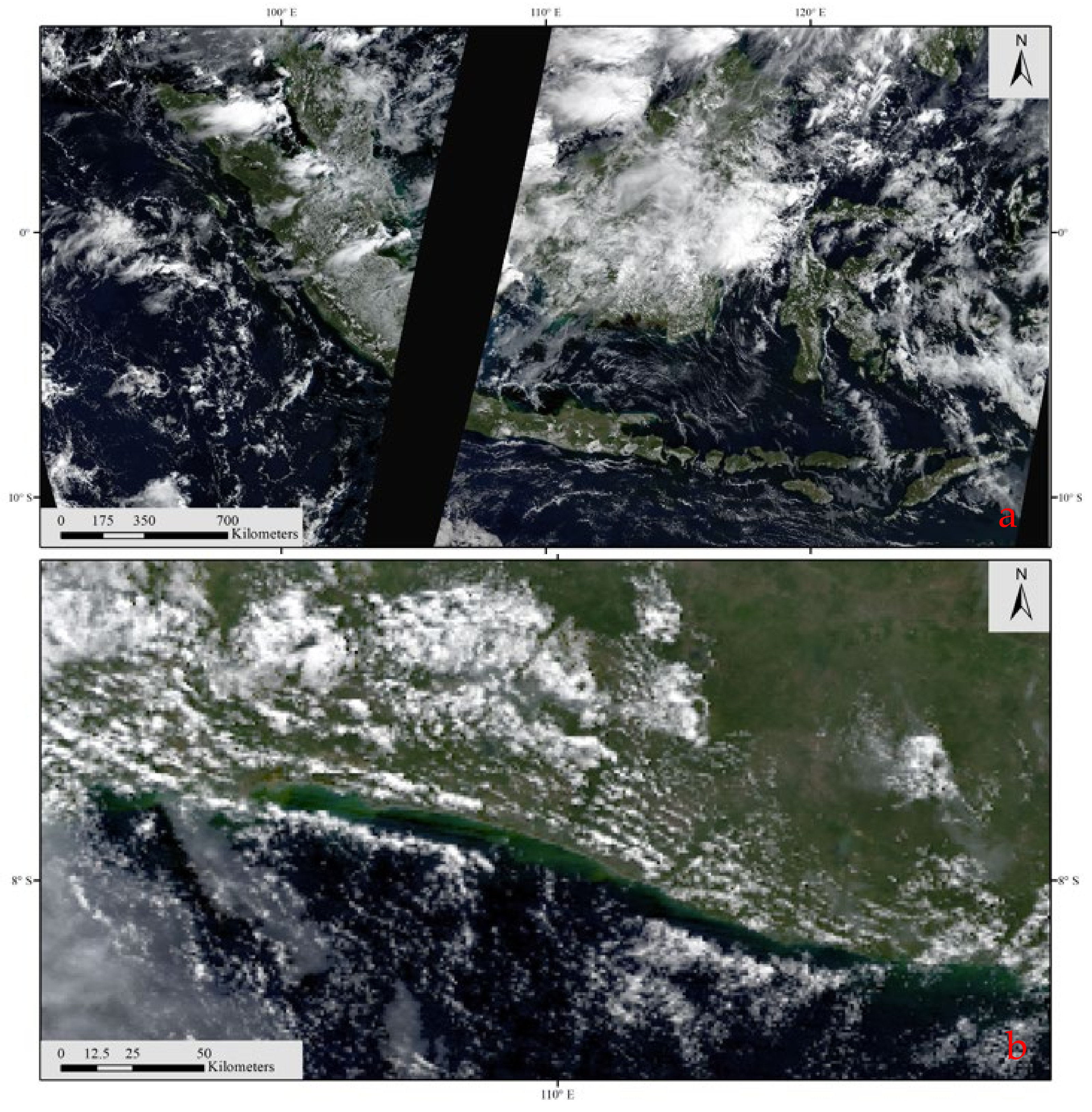
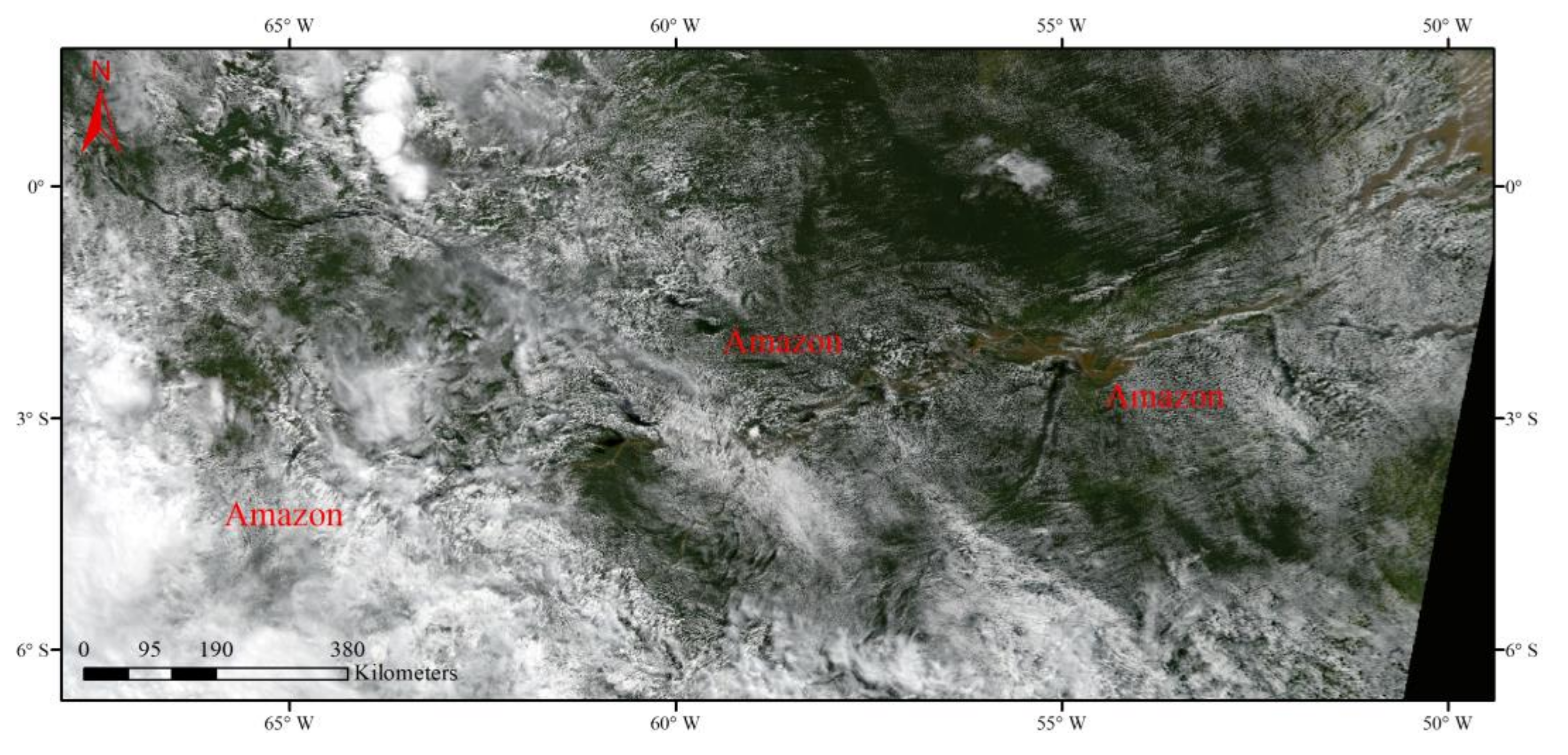
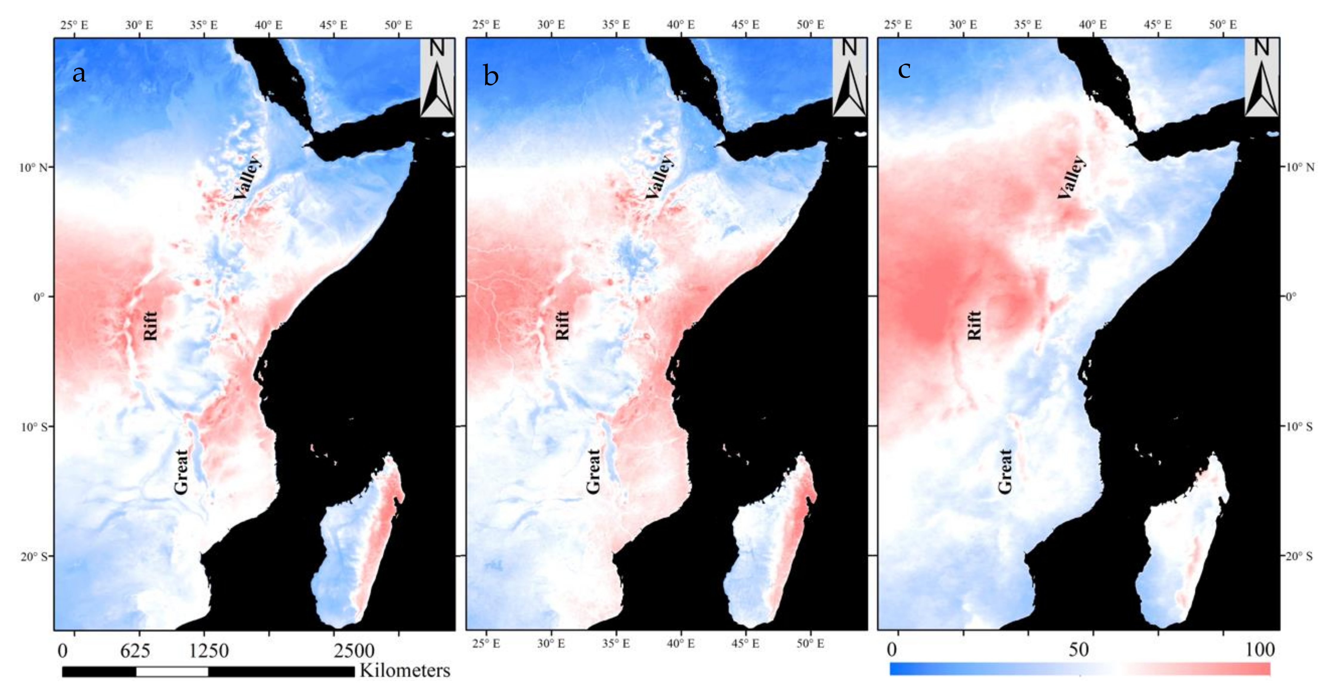
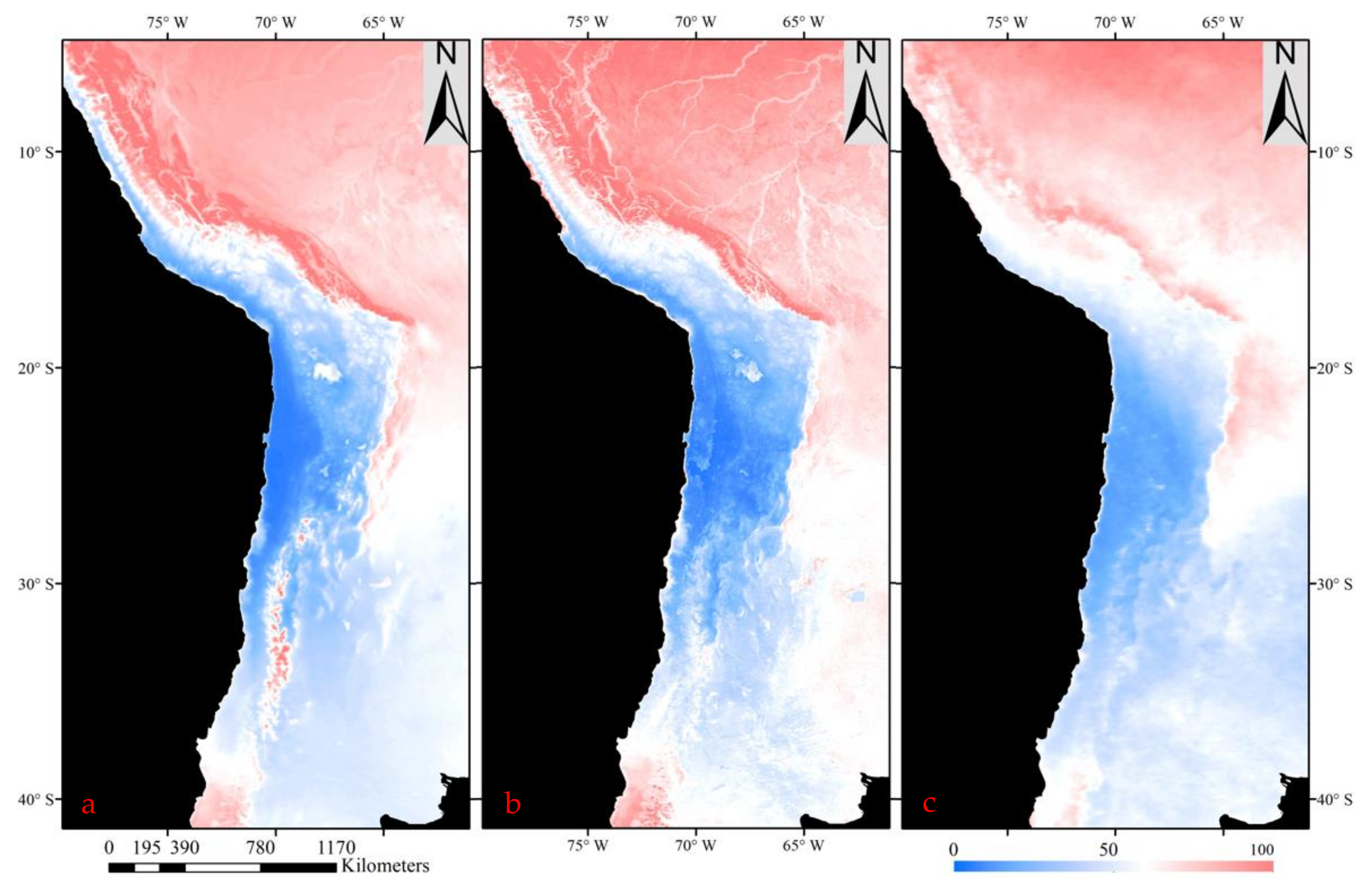
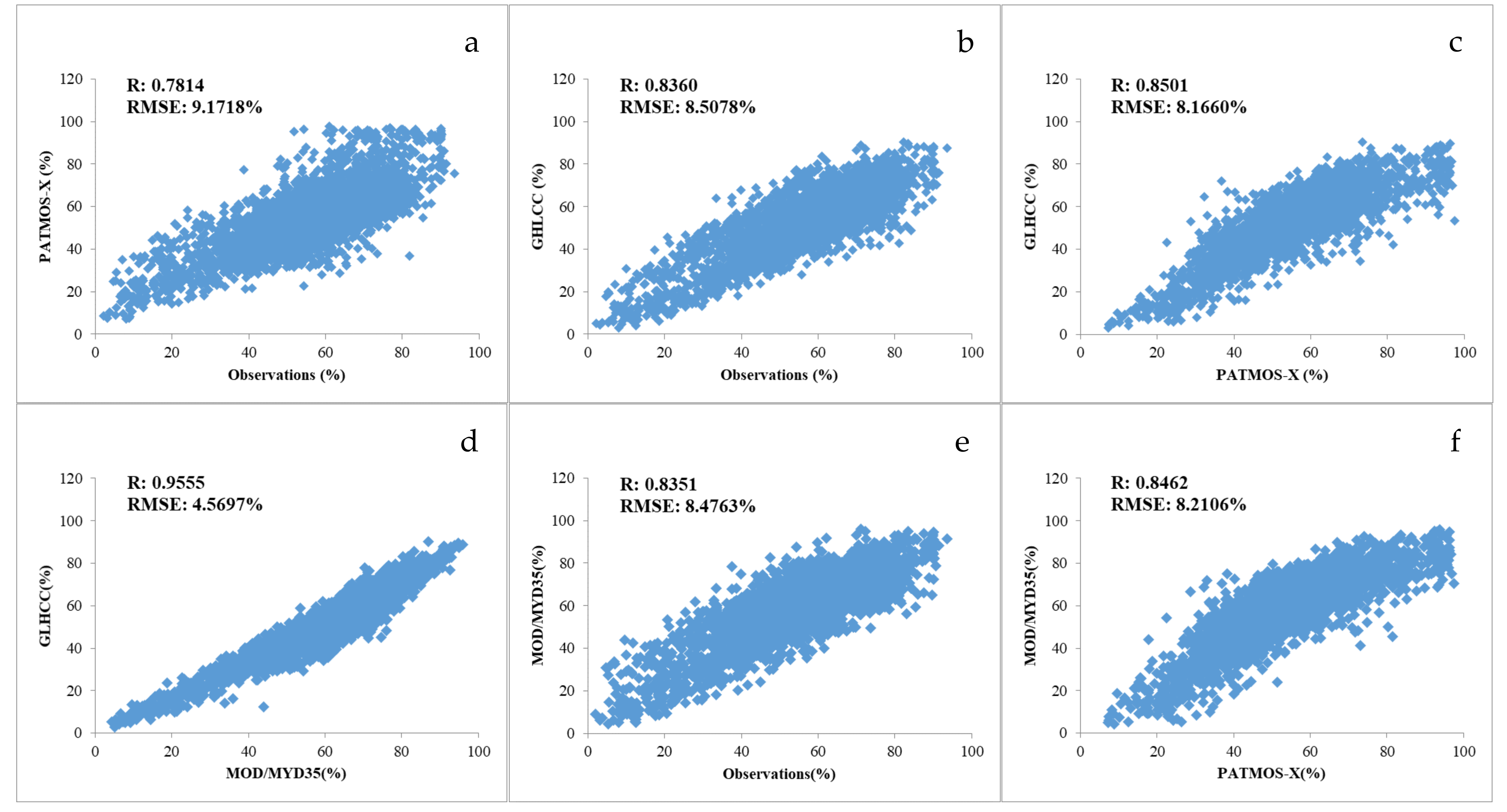
Table 1.
Statistical table of correlations between observation data and the GLHCC.
| GLHCC | 01 | 02 | 03 | 04 | 05 | 06 | 07 | 08 |
|---|---|---|---|---|---|---|---|---|
| R | 0.8771 | 0.8811 | 0.8697 | 0.8814 | 0.8722 | 0.8762 | 0.8648 | 0.8565 |
| RMSE (%) | 9.5977 | 9.2948 | 9.5694 | 9.0550 | 8.9992 | 8.7466 | 8.5865 | 8.6200 |
| GLHCC | 09 | 10 | 11 | 12 | 13 | 14 | 15 | 16 |
| R | 0.8385 | 0.8202 | 0.8101 | 0.8034 | 0.8148 | 0.8202 | 0.8250 | 0.8349 |
| RMSE (%) | 8.5485 | 8.6088 | 8.6637 | 9.0683 | 9.2785 | 9.7354 | 10.0807 | 10.4807 |
| GLHCC | 17 | 18 | 19 | 20 | 21 | 22 | 23 | 24 |
| R | 0.8627 | 0.8723 | 0.8716 | 0.8767 | 0.8856 | 0.8865 | 0.8966 | 0.8950 |
| RMSE (%) | 10.5686 | 10.9566 | 11.0265 | 10.9935 | 10.6539 | 10.4479 | 10.1088 | 9.9417 |
| GLHCC | 25 | 26 | 27 | 28 | 29 | 30 | 31 | 32 |
| R | 0.8996 | 0.9014 | 0.9041 | 0.9067 | 0.9057 | 0.9105 | 0.9029 | 0.9005 |
| RMSE (%) | 9.3886 | 8.7716 | 8.4138 | 8.2240 | 8.0853 | 7.9898 | 8.0932 | 8.3601 |
| GLHCC | 33 | 34 | 35 | 36 | 37 | |||
| R | 0.9008 | 0.8975 | 0.8815 | 0.8807 | 0.8777 | |||
| RMSE (%) | 8.5607 | 8.5896 | 9.0734 | 9.4807 | 9.8407 |
Publisher’s Note: MDPI stays neutral with regard to jurisdictional claims in published maps and institutional affiliations. |
© 2021 by the authors. Licensee MDPI, Basel, Switzerland. This article is an open access article distributed under the terms and conditions of the Creative Commons Attribution (CC BY) license (https://creativecommons.org/licenses/by/4.0/).
Share and Cite
MDPI and ACS Style
Zhang, S.; Ma, Y.; Chen, F.; Shang, E.; Yao, W.; Qiu, Y.; Liu, J. Global Land High-Resolution Cloud Climatology Based on an Improved MOD09 Cloud Mask. Remote Sens. 2021, 13, 3997. https://0-doi-org.brum.beds.ac.uk/10.3390/rs13193997
AMA Style
Zhang S, Ma Y, Chen F, Shang E, Yao W, Qiu Y, Liu J. Global Land High-Resolution Cloud Climatology Based on an Improved MOD09 Cloud Mask. Remote Sensing. 2021; 13(19):3997. https://0-doi-org.brum.beds.ac.uk/10.3390/rs13193997
Chicago/Turabian StyleZhang, Shuyan, Yong Ma, Fu Chen, Erping Shang, Wutao Yao, Yubao Qiu, and Jianbo Liu. 2021. "Global Land High-Resolution Cloud Climatology Based on an Improved MOD09 Cloud Mask" Remote Sensing 13, no. 19: 3997. https://0-doi-org.brum.beds.ac.uk/10.3390/rs13193997
Note that from the first issue of 2016, this journal uses article numbers instead of page numbers. See further details here.